CPT-2002/P.4443
Phenomenology from lattice QCD

Abstract

After a short presentation of lattice QCD and some of its current practical limitations, I review recent progress in applications to phenomenology. Emphasis is placed on heavy-quark masses and on hadronic weak matrix elements relevant for constraining the CKM unitarity triangle. The main numerical results are highlighted in boxes.

1 Introduction

The lattice formulation of quantum field theory, combined with large scale numerical simulations, is contributing in a variety of ways to the current research effort in particle physics. In the present talk I will focus on lattice QCD and its r le in quantifying non-perturbative strong interaction effects. I wish to apologize straight away to those colleagues whose work I will not be able to cover.

The objectives of lattice QCD are numerous, beginning with the goal of establishing QCD as the theory of the strong interaction in the non-perturbative domain. This can be achieved by comparing quantities calculated on the lattice, such as hadronic spectra, deep inelastic scattering structure functions, etc. to their experimentally measured counterparts. Some of these aspects were reviewed in the parallel session talk by Collins [1] and I will not repeat them here. Lattice QCD can also be used to determine the fundamental parameters of QCD, such as the strong coupling $\alpha_{s}$ or the quark masses. Because significant progress has been made in the evaluation of heavy-quark masses in the last year, I will devote a section to them. I refer you to the talk of Wittig at Lattice 2002 for a discussion of light-quark masses [2].

Another important objective of lattice QCD is to evaluate the non-perturbative, strong-interaction corrections to weak processes involving quarks. Indeed, our inability to reliably quantify these long-distance effects is often the dominant source of uncertainty in measuring fundamental weak-interaction parameters, such as the elements of the Cabibbo-Kobayashi-Maskawa (CKM) matrix. This problem has become all the more acute that the results from the CESR, LEP, the Tevatron and now the $B$ factories indicate that deviations from the standard model, if present, must be small. Since this is a natural meeting point between lattice QCD and a significant fraction of the audience, I will devote the largest part of my talk to the review of calculations of weak matrix elements relevant for constraining the unitarity triangle. This area is one where the interplay of lattice QCD and the rich experimental program of the next few years will be strong, with lattice QCD in turn contributing and improving thanks to the many precise measurements to come. In this exchange, one should not overlook the important r le that CLEO-c will play, by providing the lattice community with results of unprecedented accuracy, for $D$-meson decays in particular. Not only will these results provide stringent tests of the lattice method in the heavy-quark sector, but they will allow us to normalize our $b$-physics results by the equivalent charmed quantities, thereby reducing many of our systematic errors. I will unfortunately not have the time to discuss $D$-meson processes here and I refer you to the reviews of [13, 14] for recent summaries.

The discussion up to now certainly does not exhaust the range of subjects studied in lattice QCD. One subject of great phenomenological interest, which is not covered here, is that of non-leptonic kaon decays and direct $CP$ violation in these decays. While significant progress, both theoretical and numerical, has been made in the last years (see e.g. the reviews [5, 6, 7]), the results have not yet reached a level of maturity which permits detailed comparison with experiment. Another important subject is the r le that lattice QCD plays in understanding QCD and finite temperature and/or density. This aspect was covered by Alford in his plenary lecture at this conference [8]. Lattice QCD can also be used to make predictions for exotic hadrons, such as $b\bar{b}g$ (see e.g. [1]), and provides a powerful tool for understanding the mechanism(s) of confinement and spontaneous chiral symmetry breaking.

The remainder of the talk is organized as follows. In Sec. 2, I briefly review the lattice method and some of its current practical limitations. In Sec. 3, I discuss new developments in the computation of the charm and bottom-quark masses. I then review recent progress in the calculation of matrix elements relevant for constraining the CKM unitarity triangle in Sec. 4  and provide an outlook in Sec. 5.

2 The challenges of lattice calculations

Before reviewing some of the limitations of present day zero-temperature and zero-density lattice calculations, let me first say a few words about why lattice QCD is needed at all. As all of you know, quarks and gluons are confined within hadrons. Since confinement cannot be explained in perturbation theory, a non-perturbative tool is required to relate experiment to the underlying theory. Lattice gauge theory is a good candidate, as it provides a mathematically sound definition of non-perturbative QCD. In lattice QCD, euclidean spacetime is approximated by a discrete set of points. Quark fields reside on these points and gauge fields on the links between the points, as shown in Fig. 1. When the lattice is finite, this discretization provides both ultraviolet and infrared cutoffs and yields a well defined path integral. Because the number of degrees of freedom is finite and the integrand positive, this integral can be evaluated numerically using stochastic methods. Lattice QCD thus allows the computation of hadronic observables directly from the QCD lagrangian, i.e. from first principles. The only source of errors are the finite statistics and the discretization of spacetime. The former decrease with the square-root of the number of samples generated. The latter are proportional to powers of $a\Lambda_{\mathrm{QCD}}$ and $ap_{\mu}$, where $a$ is the lattice spacing (see Fig. 1), $\Lambda_{\mathrm{QCD}}$ is the QCD scale and $p_{\mu}$ denotes the four-momenta of the particles studied. The two errors can be made arbitrarily small, by increasing the statistics and by reducing the lattice spacing.

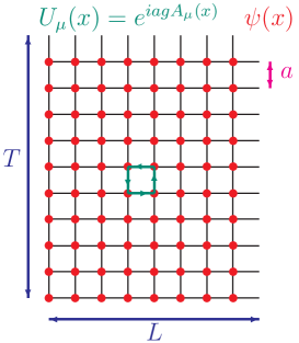
Figure 1: Two dimensional projection of a four dimensional cubic lattice. $a$ is the lattice spacing.

This is how lattice QCD works in principle. Let me now review some of the main difficulties that we encounter in practice.

2.1 Numerical cost and quenching

Though the number of degrees of freedom is finite, it is still very large. On a $32^{3}\times 64$ lattice, necessary to have a box of three-and-some fermi with an inverse lattice spacing of $2\,\mathrm{Ge\kern-1.00006ptV}$, the number of degrees of freedom is of order $10^{8}$. In addition, the cost of including sea-quark effects is very high and increases rapidly as the sea-quark mass is reduced. This explains the “popularity” of the quenched approximation, where valence quarks are treated exactly and sea-quark effects are approximated by a mean field. I will denote this approximation by $N_{f}=0$, where $N_{f}$ is the number of sea quarks included in the calculation. The benefit of this approximation, or rather truncation, is a large reduction in numerical cost since it saves calculating the very numerically intensive fermion determinant. The down side is that there is no small parameter which controls the approximation so that the size of corrections is not known a priori. Experience indicates that in many circumstances the error induced does not exceed 10 to 15%, as is shown, for instance, for the case of light-hadron masses [9]. It is clear, however, that for processes which depend dominantly on the existence of sea-quark effects, the quenched approximation will be very poor.

While significantly more costly, more and more unquenched or partially quenched  calculations are being performed. Most of them are done with two flavors of sea quarks ($N_{f}=2$), whose masses are usually substantially larger than those of the physical up and down quarks, instead of the three ($u$, $d$ and $s$, $N_{f}=3$) of our world. Furthermore, because we have much less experience with these calculations, we are still learning how to control their systematic errors.

2.2 Light quarks and chiral extrapolations

Present day algorithms become much less effective when the mass $m_{q}$ of light quarks is reduced. At the same time, unwanted finite volume effects increase. Thus at present, $N_{f}=2$ calculations are usually limited to $m_{q}{\ \lower-1.2pt\vbox{\hbox{\hbox to0.0pt{$>$\hss}\lower 5.0pt\vbox{\hbox{$\sim$}}}}\ }m_{s}/2$ or $M_{\pi}^{lat}{\ \lower-1.2pt\vbox{\hbox{\hbox to0.0pt{$>$\hss}\lower 5.0pt\vbox{\hbox{$\sim$}}}}\ }M_{K}^{expt}$, where $m_{s}$ is the strange-quark mass. This is a regime where the “$\rho$” cannot decay into two “pions”. One notable exception is the $N_{f}=3$ simulation by MILC where quark masses of about $0.2m_{s}$ are reached (see [10, 11], for instance). In any case, to reproduce the physics of $u$ and $d$ quarks, observables computed for values of $m_{q}>m_{u,d}$ must be chirally extrapolated to $m_{q}=m_{u,d}$. Can this extrapolation be performed in a controlled fashion? The only model-independent theoretical guide that we have is chiral perturbation theory ($\chi$PT). The question then becomes whether the quark masses used in simulations are light enough for $\chi$PT at low order to be applicable. The question of chiral extrapolations will be discussed more below. It was also the subject of a panel discussion at Lattice 2002 [12].

2.3 Heavy quarks and lattice artefacts

The discretization errors associated with a heavy quark are proportional to powers of $am_{Q}$, where $m_{Q}$ is the mass of this quark. For these errors to remain under control, $am_{Q}$ must be much smaller than 1, or $m_{Q}\ll a^{-1}$. Since present day inverse lattice spacings are in the range of 2 to 4 GeV, it is clear that the $b$ quark, with $m_{b}\simeq 5\,\mathrm{Ge\kern-1.00006ptV}$, cannot be simulated directly. A number of solutions to this problem exist:

$\bullet$ Relativistic quarks: calculations are performed for a number of heavy-quark masses around that of the charm, where discretization errors are under reasonable control, and the results are extrapolated in powers of $1/m_{Q}$ up to the $b$-quark mass, using heavy quark effective theory (HQET) as a guide. The drawback of this approach is that the extrapolation can be significant and that discretization errors proportional to powers of $am_{Q}$ may be amplified if this extrapolation is performed before a continuum limit is taken.

$\bullet$ Effective theories: for heavy quarks whose mass $m_{Q}$ is large compared to the other scales in the problem, denoted here by $\mu_{QCD}$, an expansion of QCD in powers of $\mu_{QCD}/m_{Q}$ can be performed. There are different implementations of this idea which go by the names of lattice HQET, of which the leading term is the static approximation, NRQCD and Fermilab approach. The important benefit of these approaches is that discretization errors are proportional to powers of $a\mu_{QCD}$ instead of powers of $am_{Q}$. The drawback is that precise calculations at the physical $b$-quark mass require the calculation of corrections proportional to powers of $1/m_{b}$, which are difficult to renormalize accurately [13]. In addition, the number of operators whose matrix elements must be computed grows rapidly with the power of $1/m_{b}$. In the case of NRQCD, one is also confronted with the fact that the continuum limit cannot be taken.

$\bullet$ Combination of relativistic and HQET results: in this case, the extrapolations from the charm and infinite heavy-quark-mass regimes are replaced by an interpolation. This is clearly a very good way to reach the $b$ quark. Discretization and renormalization errors are, however, very different in the two theories. These interpolations are thus really only reliable if the results in the two theories are obtained in the continuum limit and are non-perturbatively renormalized.

3 Heavy-quark masses

Significant progress has been made in the determination of the charm and $b$-quark masses in the last year. Unfortunately, the numerical work is still performed in the quenched approximation.

3.1 The charm-quark mass

The charm-quark mass is determined by tuning the bare heavy-quark mass in the calculation until the experimental value of an observable, such as the mass of the $D_{s}$ meson or the spin-averaged mass of the $1S$ $c\bar{c}$ states, is reproduced. The bare mass is then matched onto a continuum renormalization scheme.

The results of two new calculations appeared this year. The first [15] is a modern version of the earlier work of [16]. While the latter made use of Wilson fermions, the new calculation is performed with $\mathcal{O}\left(a\right)$-improved Wilson fermions, for which discretization errors are reduced from $\mathcal{O}\left(am_{c}\right)$ to $\mathcal{O}\left((am_{c})^{2}\right)$. This is important here since $am_{c}\sim 0.4$. Another improvement is the use of next-to-next-to-next-to-leading-log ($N^{3}LL$) results to convert the mass obtained non-perturbatively in the RI/MOM scheme at $\sim 3\,\mathrm{Ge\kern-1.00006ptV}$ to its renormalization-group invariant (RGI) [17] and ${\overline{\mbox{MS}}}$ values [18, 19]. This conversion had previously only been performed at $NLL$ order. The calculation is performed in the quenched approximation at a single value of $a^{-1}\sim 2.7\,\mathrm{Ge\kern-1.00006ptV}$. The input used to fix the charm-quark mass is the $D_{s}$ meson mass, with $m_{s}$ determined from $M_{K}$ and $a^{-1}$ from $M_{K^{*}}$. A number of systematics are considered and the result obtained is: $m^{\overline{\mbox{\tiny MS}}}_{c}(m^{\overline{\mbox{\tiny MS}}}_{c})=1.26(3)(12)\,\mathrm{Ge\kern-1.00006ptV}$.

The second calculation [20] is presumably the ultimate quenched $m_{c}$ calculation. It is also the first time the continuum limit has been thoroughly studied for this quantity. The calculation is performed at four values of the lattice spacing, ranging from approximatively 2 to 4 GeV and makes use of $\mathcal{O}\left(a\right)$-improved fermions. The input used is similar to the calculation of [15]. Five different definitions of the bare quark mass are considered. They are based on the vector Ward identity (VWI), the $\bar{c}s$-axial Ward identity (AWI) and a non-singlet $\bar{c}c$-AWI. The renormalized masses obtained from these definitions differ only by discretization errors and should therefore agree in the continuum limit. The renormalization is performed non-perturbatively la ALPHA [21], which means that the RGI mass is obtained without relying on perturbation theory below $\sim 30\,\mathrm{Ge\kern-1.00006ptV}$. The continuum extrapolation of the results for three of the definitions of the RGI mass are shown in Fig. 2, along with the results of other calculations. The discretization errors displayed by the VWI and $\bar{c}c$-AWI results are of the expected size $\sim(am_{c})^{2}$, and the RGI masses obtained from the three definitions extrapolate linearly in $a^{2}$ to surprisingly consistent values in the continuum limit, at $a=0$. Comparable agreement is found with the two other definitions. In the continuum limit the authors of [20] quote $m^{\overline{\mbox{\tiny MS}}}_{c}(m^{\overline{\mbox{\tiny MS}}}_{c})=1.301(28)(20)(7)\,\mathrm{Ge\kern-1.00006ptV}$, using the $N^{3}LL$ results of [18, 19] to convert the RGI mass to the ${\overline{\mbox{MS}}}$ scheme. The first error is a combination of statistical and a number of systematic uncertainties; the second is due to the uncertainty in $\Lambda^{(0)}_{\overline{\mbox{MS}}}$ [21]; the third is the difference of the results obtained using $N^{2}LL$ and $N^{3}LL$ expressions for the conversion from the RGI mass. In addition, a quenched scale ambiguity of $10\%$ is found to induce a 3% uncertainty on $m^{\overline{\mbox{\tiny MS}}}_{c}(m^{\overline{\mbox{\tiny MS}}}_{c})$.

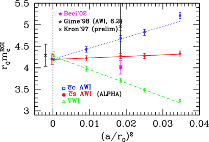
Figure 2: Continuum extrapolation of the RGI charm mass by ALPHA [20]. All quantities are plotted in units of the scale $r_{0}\simeq 0.5\,\mathrm{fm}$ [22]. The vertical dashed line corresponds to the continuum limit. The other results are: Beci’02 [15], Gime’98 [16] and Kron’97 [23]. Not shown is a result obtained from combining sumrule techniques with lattice results [24].

Before concluding on the charm-quark mass, let me mention that Juge et al. [25] are performing a modern version of Kronfeld’s preliminary 1997 calculation [23], where the spin-averaged mass of the $1S$ $c\bar{c}$-states was used to tune $m_{c}$ and the lattice spacing was determined from the $1P-1S$ splitting. In this new calculation, performed at several lattice spacings, the mass is renormalized perturbatively at $N^{2}LO$ instead of at $NLO$.

My conclusion for the charm-quark mass is that the result of [20] is the quenched result. So I use it as the central value and add to it a 15% systematic error to account for quenching uncertainties. Thus, I quote as a lattice summary number,

$$m^{\overline{\mbox{\tiny MS}}}_{c}(m^{\overline{\mbox{\tiny MS}}}_{c})=1.30(4)(20)\,\mathrm{Ge\kern-1.00006ptV}\ .$$

Because of the large quenching uncertainty, this result does not improve on the 2002 PDG summary, $1.0\,\mathrm{Ge\kern-1.00006ptV}\leq m^{\overline{\mbox{\tiny MS}}}_{c}(m^{\overline{\mbox{\tiny MS}}}_{c})\leq 1.4\,\mathrm{Ge\kern-1.00006ptV}$, which does not include lattice results [26]. It is clear that the error on $m_{c}$ from the lattice can only be reduced now with an unquenched calculation.

3.2 The $b$-quark mass

Since the $b$-quark mass is the $B$-meson mass up to a smallish correction, what we really want is an accurate calculation of this correction. This statement is all the more relevant that the $b$-quark mass cannot be reached in large volumes on present day lattices. Thus we rely on the heavy-quark expansion of the $B$-meson mass:

$$\begin{array}[]{rccl}M_{B}&=&m^{\mbox{\tiny bare}}_{b}&+\mathcal{E}+\mathcal{O}\left(\frac{\Lambda_{\mathrm{QCD}}^{2}}{m_{b}}\right)\\ &=&m^{\mbox{\tiny pole}}_{b}-\delta m&+\mathcal{E}+\mathcal{O}\left(\frac{\Lambda_{\mathrm{QCD}}^{2}}{m_{b}}\right)\end{array}\ ,$$ (1)

where the residual mass $\delta m$ and the bare binding energy $\mathcal{E}$ are linearly divergent individually, but this divergence cancels in the difference.

What the heavy-quark expansion seeks to achieve is a separation of short and long-distance contributions to $M_{B}$. In Eq. (1), $\mathcal{E}$ is meant to contain the long-distance components of $M_{B}$ and $m_{b}^{bare}$, the short-distance contributions. This division can be made unambiguous with a hard cutoff, such as the lattice spacing, and $\mathcal{E}$ can be computed in the static approximation on lattices which are not particularly fine.

Two approaches to the determination of $m_{b}$ have been pursued in the context of HQET: a “perturbative” one [27] and a non-perturbative one. The latter was proposed in the last year [28, 29] and represents an important theoretical development in the matching of HQET to QCD.

3.2.1 The “perturbative” approach

In this approach, the determination of $m_{b}$ proceeds in three steps:

a) $\mathcal{E}$ is evaluated numerically in the static approximation;

b) $\delta m$ is calculated in lattice-HQET perturbation theory; it is known to three loops for $N_{f}=0$ [30, 31] and two loops for $N_{f}\neq 0$ [32];

c) the $b$-quark mass is then obtained through

$$m^{\overline{\mbox{\tiny MS}}}_{b}(m^{\overline{\mbox{\tiny MS}}}_{b})=c(m^{\overline{\mbox{\tiny MS}}}_{b})(M_{B}+\delta m-\mathcal{E})+\mbox{\small$\mathcal{O}\left(\frac{\Lambda_{\mathrm{QCD}}^{2}}{m_{b}}\right)$}\ ,$$

where $c(m^{\overline{\mbox{\tiny MS}}}_{b})$ is known to three-loop accuracy [33].

The problems with this approach are:

$\bullet$ that the cancellation of power divergences between $\mathcal{E}$ and $\delta m$ is not complete: $\mathcal{E}-\delta m\sim\alpha_{s}^{n}/a$ ($n{=}3$ for N²LO calculations) which becomes large in the continuum limit;

$\bullet$ $\delta m$ has a renormalon ambiguity of order $\Lambda_{\mathrm{QCD}}$ which cancels against the one in $c(m^{\overline{\mbox{\tiny MS}}}_{b})$ [34, 35].

Both these problems require one to go to high order in perturbation theory. That this is not only a conceptual problem can be inferred from the fact that the uncertainty which the neglect of higher-order terms induces on $m^{\overline{\mbox{\tiny MS}}}_{b}(m^{\overline{\mbox{\tiny MS}}}_{b})$ is about 200 MeV at NLO, 100 MeV at N²LO and 50 MeV at N³LO, for $N_{f}=0$.

The first problem further means that a continuum limit is not possible. Thus, one is left with discretization errors proportional to powers of $a\Lambda_{\mathrm{QCD}}$ and perturbative errors of order $\alpha_{s}^{3}$ for N²LO calculations.

3.2.2 The non-perturbative approach

This approach was proposed very recently by Heitger and Sommer [28, 29]. It provides a framework in which to match HQET and QCD fully non-perturbatively and in the continuum limit. In that sense it solves all of the problems of the perturbative method.

Since this development is interesting conceptually, it is worth trying to get the main idea across. It is, however, rather technical and I will only provide a sketch here:

a) First observe that the bare quark mass 

$$m^{\mbox{\tiny bare}}(m^{{\mbox{\tiny RGI}}},a)=M(L_{0},m^{{\mbox{\tiny RGI}}},a)-\mathcal{E}(L_{0},a)$$ (2)

$$+\mathcal{O}\left(1/L_{0}^{2}m^{{\mbox{\tiny RGI}}},\Lambda_{\mathrm{QCD}}/L_{0}m^{{\mbox{\tiny RGI}}},\Lambda_{\mathrm{QCD}}^{2}/m^{{\mbox{\tiny RGI}}}\right)\ ,$$

which is a parameter in the HQET lagrangian, knows nothing about $L_{0}$, the size of the lattice considered. It is only a function of the RGI quark mass and the lattice spacing $a$. In Eq. (2), $M(L_{0},m^{{\mbox{\tiny RGI}}},a)$ is a quantity with mass-dimension one which becomes the mass $M$ of the heavy-light meson containing a heavy quark of mass $m^{{\mbox{\tiny RGI}}}$ in the limit $L_{0}\to\infty$ and $a\to 0$.

The independence of $m^{\mbox{\tiny bare}}$ on $L_{0}$ means that when $m^{{\mbox{\tiny RGI}}}\sim m^{{\mbox{\tiny RGI}}}_{b}$, it can be studied on small $(1/\Lambda_{\mathrm{QCD}}\geq L_{0}\gg 1/m^{{\mbox{\tiny RGI}}}_{b})$ and fine-grained $(am^{{\mbox{\tiny RGI}}}_{b}\ll 1)$ lattices where discretization errors proportional to powers of $\sim am^{{\mbox{\tiny RGI}}}_{b}$ are small.

b) The second step consists in equating $m^{\mbox{\tiny bare}}(m^{{\mbox{\tiny RGI}}},a)$, defined through Eq. (2), on a small ($L_{0}$) and large ($L$) box:

$$M\simeq\mathcal{E}(L,a)-\mathcal{E}(L_{0},a)+M(L_{0},m^{{\mbox{\tiny RGI}}},a)\ ,$$ (3)

where I have assumed that $L$ is large enough and $a$ small enough for $M(L,m^{{\mbox{\tiny RGI}}},a)$ to be the meson mass $M$ to good approximation. It is this mass which is going to be set to the experimental value of the $B$-meson mass to determine $m^{{\mbox{\tiny RGI}}}_{b}$.

c) Zero is then inserted into the right-hand side of Eq. (3), in the following way:

$$M \simeq \mathcal{E}(L,a)-\mathcal{E}(L_{n},a)+\cdots-\mathcal{E}(L_{1},a)$$

$$+ \mathcal{E}(L_{1},a)-\mathcal{E}(L_{0},a)+M(L_{0},m^{{\mbox{\tiny RGI}}},a)\ ,$$

where one takes $L=L_{n+1}>L_{n}=2^{n}L_{0}>\cdots>L_{0}$. The trick is to note that one can consider a sequence of lattice spacings, $a\leq a_{0}\leq\cdots\leq a_{n}\ll 1/\Lambda_{\mathrm{QCD}}$, and that as long as $a_{i}/L_{i}\ll 1$, Eq. (3.2.2) is equivalent to

$$M \simeq \mathcal{E}(L,a_{n})-\mathcal{E}(L_{n},a_{n})+\cdots-\mathcal{E}(L_{1},a_{1})$$

$$+ \mathcal{E}(L_{1},a_{0})-\mathcal{E}(L_{0},a_{0})+M(L_{0},m^{{\mbox{\tiny RGI}}},a)\ ,$$

up to small discretization errors proportional to powers of $a_{i}/L_{i}$ and $a_{i}\Lambda_{\mathrm{QCD}}$. This breaks up the problem of having to accommodate long-distance physics on a scale $L$ and short-distance effects associated with the scale $1/m^{{\mbox{\tiny RGI}}}_{b}$ into a sequence of more manageable problems. Indeed, for each binding energy difference $\Delta\mathcal{E}_{i}=\mathcal{E}(L_{i+1},a_{i})-\mathcal{E}(L_{i},a_{i})$, $i=0,\cdots,n$, the power divergences $\sim 1/a_{i}$ in $\mathcal{E}(L_{i+1},a_{i})$ and $\mathcal{E}(L_{i},a_{i})$ cancel and the range of scales involved, from $a_{i}$ to $L_{i+1}$, is not too large.

d) This means that the $\Delta\mathcal{E}_{i}$ can be computed at leading order in lattice HQET on the sequence of lattices illustrated in Fig. 3. Furthermore, in each step of the sequence, the continuum limit $a_{i}\to 0$ can be taken.

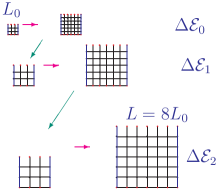
Figure 3: Sequence of lattices on which the binding-energy differences, $\Delta\mathcal{E}_{i}$, are computed.

e) Next compute $M(L_{0},m^{{\mbox{\tiny RGI}}},a)$ in lattice QCD for $m^{{\mbox{\tiny RGI}}}\sim m^{{\mbox{\tiny RGI}}}_{b}$, taking $a\to 0$. This is possible, since the range of scales involved $a\ll 1/m^{{\mbox{\tiny RGI}}}_{b}\ll L_{0}$ is not too large. Then, interpolate $M(L_{0},m^{{\mbox{\tiny RGI}}},0)$ to the value of $m^{{\mbox{\tiny RGI}}}$ which solves

$$M(L_{0},m^{{\mbox{\tiny RGI}}},0)=M_{B}-\sum_{i=0}^{n}\Delta\mathcal{E}_{i}\ .$$ (6)

This yields $m^{{\mbox{\tiny RGI}}}=m^{{\mbox{\tiny RGI}}}_{b}+\mathcal{O}\left(1/L_{0}^{2}m^{{\mbox{\tiny RGI}}}_{b},\cdots\right)$. $m^{{\mbox{\tiny RGI}}}_{b}$ can be then converted to $m^{\overline{\mbox{\tiny MS}}}_{b}$ using $N^{3}LL$ running [18, 19] if necessary. The authors of [28] choose $L_{0}\simeq 0.2\,\mathrm{fm}$, $n=2$, $L\simeq 1.5\mathrm{fm}\sim 2^{3}L_{0}$ and use $M_{B_{s}}$ instead of $M_{B}$ to tune to $m^{{\mbox{\tiny RGI}}}_{b}$.

The great benefit of this approach is that $m^{{\mbox{\tiny RGI}}}_{b}$ is obtained without discretization nor perturbative errors, in contrast to the “perturbative” approach described earlier. Power corrections to the heavy-quark limit, however, are still present (see Eq. (2)). Those involving $1/L_{0}m^{{\mbox{\tiny RGI}}}_{b}$ are peculiar to this finite-volume approach and their size should be investigated carefully.

Other approaches, based on lattice NRQCD and a study of upsilon [36, 37] or heavy-light [38] spectra, have also been explored. These calculations were performed using NLO perturbation theory and are therefore less accurate than present day calculations.

Having presented the various approaches used to determine the $b$-quark mass on the lattice, I now review the results obtained. These results are summarized in Fig. 4. Only published results are presented. The exception being the only fully non-perturbative result of [28, 29] and the unquenched, $N_{f}=2$, result of [37], the latter because it enables an estimate of quenching uncertainties.

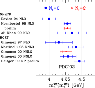
Figure 4: Lattice results for the $b$-quark mass: Davies 94 [36], Hornbostel 98 [37], Ali Khan 99 [38], Gimenez 97 [39], Martinelli 98 [32], Gimenez 00 [40], Heitger 02 [28, 29]. Next to the reference is the order in perturbation theory used in the calculation. NP stands for non-perturbative. The vertical lines delimit the range given by the PDG [26].

Not shown are preliminary quenched, N³LO results which were obtained using NRQCD and an extrapolation to the infinite-mass limit [1, 41]. At this same N³LO order, the result of a preliminary quenched HQET calculation was reported in [42]. Both these results are compatible with the N²LO results of [40], but have a perturbative uncertainty about twice as small ($\sim 50\,\mathrm{Me\kern-1.00006ptV}$).

The only unquenched results available [40, 37, 41] show little change compared to the corresponding quenched results. However, the masses of the sea quarks considered are rather large. In [40], for instance, the calculation is performed for two values of the sea-quark mass, $m_{sea}$, in the interval $m_{s}/2$ to $m_{s}$. These findings should be checked through further unquenched studies.

Performing a simple average of the quenched $\beta=6.2$ result of [40] and the preliminary non-perturbative result of [28, 29] yields

$$m^{\overline{\mbox{\tiny MS}}}_{b}(m^{\overline{\mbox{\tiny MS}}}_{b})=4.38(9)(10)\,\mathrm{Ge\kern-1.00006ptV}\ ,$$

where the first error is typical of the quenched calculations considered, chosen also to accommodate the two values within one standard deviation, and the second is an estimate of the remaining quenching uncertainty, taken to be 10% of the $B_{s}$ binding energy. The quenching error was reduced from the 15% used for the charm mass to 10% because of the evidence provided by the $N_{f}=2$ results discussed above.

4 Lattice QCD for the unitarity triangle

Analyses of the CKM unitarity triangle (UT) have come to rely more and more on weak matrix elements calculated in lattice QCD (please see Stocchi’s plenary review [43] and e.g. [44, 45]). In these analyses, the summit $(\bar{\rho},\bar{\eta})$ of the UT is constrained through $\Delta m_{d}$, the frequency of $B^{0}_{d}-\bar{B}^{0}_{d}$ oscillations, $\Delta m_{d}/\Delta m_{s}$, the ratio of this frequency to the one for $B^{0}_{s}-\bar{B}^{0}_{s}$ oscillations, $\epsilon_{K}$ which parametrizes indirect $CP$ violation in $K\to\pi\pi$ decays and the ratio $|V_{ub}/V_{cb}|$, together with the value of $\sin 2\beta$ determined from the time-dependent $CP$ asymmetry in $B\to J/\psi K_{S}$. The theoretical expressions for $\Delta m_{d}$, $\Delta m_{s}/\Delta m_{d}$ and $\epsilon_{K}$ involve CKM factors and short-distance Wilson coefficients which are known to NLO in perturbation theory (see e.g. [46] for a review). They also contain the non-perturbative QCD quantities $f_{B_{d}}^{2}B_{B_{d}}$, $\xi^{2}=\frac{f_{B_{s}}^{2}B_{B_{s}}}{f_{B_{d}}^{2}B_{B_{d}}}$ and $B_{K}$. These quantities are defined through the matrix elements:

$$\langle\bar{B}_{q}|(\bar{b}q)_{V-A}(\bar{b}q)_{V-A}|B_{q}\rangle=\frac{8}{3}M_{B_{q}}^{2}f_{B_{q}}^{2}B_{B_{q}}\ ,$$ (7)

$$\langle 0|\bar{b}\gamma_{\mu}\gamma_{5}q|B_{q}(p)\rangle=ip_{\mu}f_{B_{q}}\ ,\hskip 66.86414pt$$ (8)

$$\langle\bar{K}^{0}|(\bar{s}d)_{V-A}(\bar{s}d)_{V-A}|K^{0}\rangle=\frac{8}{3}M_{K}^{2}f_{K}^{2}B_{K}\ ,$$ (9)

with $q=d$, $s$. It is for the calculation of these matrix elements that lattice QCD is used.

In addition to the matrix elements mentioned above, lattice QCD can also be used to obtain the form factors relevant for $B\to D^{*}(D)\ell\nu$ and $B\to\pi(\rho)\ell\nu$. Together with these form factors, experimental measurements of the corresponding differential decay rates enable independent determinations of $|V_{cb}|$ and $|V_{ub}|$, respectively.

4.1 $B_{q}-\bar{B}_{q}$–mixing: $f_{B_{q}}$

Though $f_{B_{q}}$ and $B_{B_{q}}$ are correlated through the $\Delta B=2$ matrix element of Eq. (7), it is useful to review these quantities separately: once measured, leptonic decays of $B^{+}$, which are governed by $f_{B}$, will allow a clean determination of $|V_{ub}|$; there exist many more calculations of $f_{B_{q}}$; systematics on $f_{B_{q}}$ and $B_{B_{q}}$ are quite different.

In Fig. 5, I have compiled all recent results for $f_{B}$ , both quenched and unquenched. A similar compilation for $f_{B_{s}}/f_{B}$ is shown in Fig. 6.

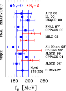
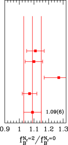
Figure 5: Lattice results for the decay constant of the $B$ meson in quenched ($N_{f}=0$) and unquenched QCD ($N_{f}=2$) (left) and their ratio (right). Calculations are grouped by the approach used for the heavy quark. Only results published after 1996 are shown. These are: APE 00 [47], LL 00 [48], UKQCD 00 [49], FNAL 97 [50], CP-PACS 00 [51], MILC 02 [52] , Ali Khan 98 [53], Collins 99 [54], CP-PACS 01 [55], JLQCD 02 [65]. Also shown are my averages of the results for $f_{B}^{N_{f}=0}$ and $f_{B}^{N_{f}=2}/f_{B}^{N_{f}=0}$.

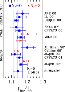
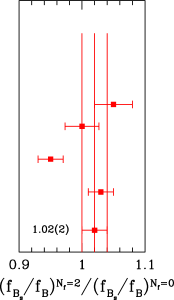
Figure 6: As in Fig. 5, but for $f_{B_{s}}/f_{B}$ and $(f_{B_{s}}/f_{B})^{N_{f}=2}/(f_{B_{s}}/f_{B})^{N_{f}=0}$.

From these figures it is clear that results obtained with different approaches to treating heavy quarks (relativistic QCD vs effective theories) agree fairly well, suggesting that the heavy-quark-mass dependence of these quantities is under control.

The figures also indicate that $N_{f}=2$ calculations show an increase in $f_{B}$ over its quenched value of up to $\mathcal{O}\left(15\%\right)$ while these effects appear to be small in $f_{B_{s}}/f_{B}$. These trends are confirmed by MILC who recently presented the first results of a calculation performed with three flavors of sea quarks ($N_{f}=3$) [10, 11]. Their preliminary findings are $f_{B}^{N_{f}=3}>f_{B}^{N_{f}=2}$ and $f_{B}^{N_{f}=3}/f_{B}^{N_{f}=0}=1.23(4)(6)$ and $(f_{B_{s}}/f_{B})^{N_{f}=3}=1.18(1)^{+4}_{-1}$.

Before embarking on a discussion of systematic errors, I wish to briefly mention that an interesting finite-volume technique for computing $B$-meson decay constants was presented very recently [56]. The first quenched results obtained using this method are $f_{B}=170(11)(5)(22)\,\mathrm{Me\kern-1.00006ptV}$ and $f_{B_{s}}=192(9)(5)(24)\,\mathrm{Me\kern-1.00006ptV}$ [56].

4.1.1 $f_{B_{q}}$: chiral extrapolations

In the quenched approximation, the calculation of $f_{B}$ requires a chiral extrapolation in light-valence-quark mass from $m_{val}{\ \lower-1.2pt\vbox{\hbox{\hbox to0.0pt{$>$\hss}\lower 5.0pt\vbox{\hbox{$\sim$}}}}\ }m_{s}/2$ to $m_{u,d}$. In unquenched calculations, an additional chiral extrapolation in sea-quark mass from $m_{sea}{\ \lower-1.2pt\vbox{\hbox{\hbox to0.0pt{$>$\hss}\lower 5.0pt\vbox{\hbox{$\sim$}}}}\ }m_{s}/2$ to $m_{u,d}$ is needed to obtain both $f_{B}$ and $f_{B_{s}}$. All of the results presented in the figures above assume mild extrapolations. It is legitimate to ask whether the chiral behavior of $f_{B}$ and $f_{B_{s}}$ is well understood. This is a serious issue for UT fits, due to the importance of the $\Delta m_{s}/\Delta m_{d}$ constraint.

According to $N_{f}=2$ heavy meson chiral perturbation theory (HM$\chi$PT), the light-quark-mass behavior of $f_{B}$, where the mass of light valence and sea quarks are identified ($m_{val}=m_{sea}$), is given by [57]

$$\frac{f_{B}\sqrt{M_{B}}}{\phi_{B}^{(0)}}=1-\frac{3}{4}(1+3g^{2})\left[\frac{M_{SS}}{4\pi f}\right]^{2}\ln\frac{M_{SS}^{2}}{\Lambda_{f_{B}}^{2}},$$ (10)

at leading order in the $1/M_{B}$ expansion and up to NNLO chiral corrections. In Eq. (10), $\phi_{B}^{(0)}$ is the value of $f_{B}\sqrt{M_{B}}$ in the combined heavy-quark and chiral limits, $g$ is the $B^{*}B\pi$ coupling in this same limit, $M_{SS}$ is the mass of a pseudoscalar meson composed of a quark and anti-quark of mass $m_{sea}$, $f$ is the pion decay constant in the chiral limit and $\Lambda_{f_{B}}$ is a scale which parametrizes the unknown coupling of the contact term proportional to $M_{SS}^{2}$.  For $f_{B_{s}}$ and $N_{f}=2$, one has to resort to partially quenched HM$\chi$PT, since the valence and sea light quarks are not degenerate. The prediction for the sea-quark-mass dependence of $f_{B_{s}}$ is [58] ($m_{val}$ fixed to $m_{s}$)

$$\frac{f_{B_{s}}\sqrt{M_{B_{s}}}}{\phi_{B_{s}}^{(0)}}=1-(1+3g^{2})\left[\frac{M_{VS}}{4\pi f}\right]^{2}\ln\frac{M_{VS}^{2}}{\Lambda_{f_{B_{s}}}^{2}},$$ (11)

at leading order in the $1/M_{B}$ expansion and up to NNLO chiral corrections. In Eq. (11), $M_{VS}$ is the mass of a pseudoscalar meson composed of quarks of mass $m_{val}=m_{s}$ and $m_{sea}$. The dependence on sea-quark mass is recovered through the LO $\chi$PT relation, $M_{VS}^{2}=(M_{SS}^{2}+M_{VV}^{2})/2$. This dependence is much milder for $f_{B_{s}}$ than it is for $f_{B}$, because $M_{VS}$ is much less sensitive to $m_{sea}$ than is $M_{SS}$.

CLEO has recently determined $g_{c}=0.59(7)$ using its measurement of the $D^{*+}$ width. $g_{c}$ is the $D^{*}D\pi$ coupling and differs from $g$ by chiral and $1/M_{D}$ corrections. This value is consistent with a recent lattice calculation which further finds little dependence of the $D^{*}D\pi$ coupling on the charm quark mass [60]. However, agreement amongst different determinations of $g$ is generally rather poor, the spread of which lies in the interval $0.2<g<0.7$ [61, 62, 63].

JLQCD have achieved an impressive statistical accuracy for their $N_{f}=2$ determinations of $f_{B}$ and $f_{B_{s}}$ [64]. This has enabled them to study rather extensively the dependence of these quantities on light-quark mass.  These preliminary studies are illustrated in Fig. 7, where the quantities $f_{B}\sqrt{M_{B}}$ and $f_{B_{s}}\sqrt{M_{B_{s}}}$ are plotted against $M_{SS}^{2}$. In the quenched case, where no sea quarks are present, $f_{B_{val}}\sqrt{M_{B_{val}}}$ is a function of $M_{VV}^{2}$. In fact, the near linearity of these quenched results, observed in all such calculations, is one of the reasons why chiral extrapolations have been done assuming mild light-quark-mass dependence.

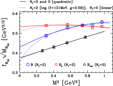
Figure 7: Preliminary results for the dependence of $f_{B_{(s)}}\sqrt{M_{B_{(s)}}}$ ($f_{B_{val}}\sqrt{M_{B_{val}}}$) on light-quark (valence-quark) mass in $N_{f}=2$ ($N_{f}=0$) NRQCD [64] ([69]). $M\equiv M_{SS}$ for $N_{f}=2$ and $M\equiv M_{VV}$ when $N_{f}=0$. The curves denoted log correspond to fits to Eqs. (10) and (11).

JLQCD perform a number of fits to their results for $f_{B}\sqrt{M_{B}}$ and $f_{B_{s}}\sqrt{M_{B_{s}}}$ versus $M_{SS}^{2}$, including fits to the HQ$\chi$PT expressions of Eqs. (10) and (11) [64].  For $f_{B_{s}}\sqrt{M_{B_{s}}}$, Fig. 7 indicates that the extrapolated value at $M_{SS}^{2}=M_{\pi}^{2}$ is affected only mildly by the presence of chiral logs. The situation is radically different for $f_{B}\sqrt{M_{B}}$ where the extrapolated value depends critically on the coupling $g$, becoming lower for larger values of $g$. For $g=0.6$, JLQCD find that the extrapolated value of $f_{B}\sqrt{M_{B}}$ is 17% lower than that obtained through a quadratic fit in $M_{SS}^{2}$ [65]. They conclude that the inclusion of logarithms in these chiral extrapolations could significantly lower the value of $f_{B}$ and increase that of $f_{B_{s}}/f_{B}$. Similar conclusions were reached about $f_{B_{s}}/f_{B}$ by the authors of [66], using the predicted $N_{f}=3$ chiral logs and information from lattice calculations. Based on these observations Yamada, who reviewed heavy-quark physics at Lattice 2002, chose to quote for $f_{B}$ a central value taken from linear/quadratic chiral extrapolations, adding to it a $-17\%$ systematic error to account for possible effects of chiral logs [65]. Given the size of this error and its effect on UT fits, I wish to make a number of comments on the JLQCD analyses:

$\bullet$ The chiral log extrapolation of the results of JLQCD for $f_{B}\sqrt{M_{B}}$ is problematic from a numerical analysis point of view in the sense that this functional form varies most rapidly in a region unconstrained by data.

$\bullet$ The size of the NLO chiral correction of Eq. (10) is $\mathcal{O}\left(60\%\right)$ at the heaviest point. With such a sizeable correction, higher-order terms cannot be ignored. Moreover, $\chi$PT is not expected to hold up to $1\,\mathrm{Ge\kern-1.00006ptV}$ since the expansion is in $M_{SS}^{2}$ over $8\pi^{2}f^{2}\simeq(1.1\,\mathrm{Ge\kern-1.00006ptV})^{2}$.

$\bullet$ Another important piece of information is the behavior of $f_{\pi}$ vs $M_{\pi}^{2}$ obtained by JLQCD with the same gauge configurations [64]. While the coefficient of the chiral log in the $\chi$PT expression for $f_{\pi}$ [67] may even be larger than the one for $f_{B}\sqrt{M_{B}}$ (2 vs the 1.6 obtained for $g=0.6$), their nearly linear results for $f_{\pi}$ are inconsistent with NLO chiral behavior ($\chi^{2}/dof=5.1$) [64] in the range of sea quark masses where they claim that logarithmic behavior may have been observed for $f_{B}\sqrt{M_{B}}$.

$\bullet$ Because JLQCD work at fixed bare gauge coupling and with a fixed number of lattice sites, the spacing and the volume of their lattice shrink by roughly 25% as $M_{SS}^{2}$ varies from $\sim 1\,\mathrm{Ge\kern-1.00006ptV}^{2}$ to $\sim 0.3\,\mathrm{Ge\kern-1.00006ptV}^{2}$. This rather large variation will amplify the unphysical dependence on $M_{SS}^{2}$ induced by mass-dependent finite-volume and discretization errors.

$\bullet$ If instead of requiring that the NLO behavior of Eq. (10) be applicable all the way up to $M_{SS}^{2}\sim 1\,\mathrm{Ge\kern-1.00006ptV}^{2}$, one models the possible effect of higher-order chiral terms, allowing or not the logarithmic behavior to set in at lower masses, one finds that the downward shift in JLQCD’s results for $f_{B}$ due to chiral logs is generically less than about 10% (for $g\leq 0.6$). For $f_{B_{s}}$, a similar analysis gives variations which are negligible compared to other systematics.

It is important to note, also, that the uncertainty due to chiral logs depends on the details of the calculation and, in particular, on whether the lattice spacing was set with a quantity which is sensitive to chiral logs and whether these logarithms were taken into account. This means that one cannot generically ascribe a chiral-log error to quantities such as $f_{B}$. However, the quenched results reviewed above, which form the basis of the summary numbers presented below, include an error associated with scale setting and agree within errors despite the fact that different groups set the scale with quantities which have varying degrees of sensitivity to chiral logs. This indicates that the chiral-log uncertainty due to scale setting is to some extent already accounted for. The same appears to be true for the $N_{f}=2$ over $N_{f}=0$ ratios which are also used to obtain the final summary numbers. Thus, I will assume that the discussion surrounding the chiral behavior of the JLQCD results can be used to obtain a rough estimate of the range of deviations that could be induced by the chiral logs intrinsic to $f_{B}$ and $f_{B_{s}}$. Given that discussion, the exploratory nature of the investigations of chiral-log effects, it seems reasonable to fix the central values of $f_{B}$ and $f_{B_{s}}$ from linear/quadratic chiral extrapolations and to add a $-10\%$ systematic error to $f_{B}$ to account for the uncertainty in the chiral extrapolation and none to $f_{B_{s}}$.

To reduce the chiral-log error in future analyses, the obvious solution is to extend the lattice results to smaller masses to match unambiguously onto NLO chiral behavior. This is numerically very costly, however.  In the meantime, it would be helpful to chirally extrapolate dimensionless ratios of quantities in which the chiral logs cancel or nearly cancel. For such ratios, the uncertainties due to contributions of chiral logarithms at small light-quark mass will be much reduced. For $f_{B}$ in $N_{f}{=}2$ calculations, and $g$ around 0.6, a good candidate would be $f_{B}/f_{\pi}$ (see discussion above and also [52]).  To make such analyses reliable, it is important to treat chiral logarithms consistently throughout the calculation [52], not to consider light quarks which are too massive, to reduce the uncertainty on $g$ and to determine the extent to which $1/M_{B}$ corrections can modify the prediction of Eq. (10). It is also important to verify that variations in lattice spacing and volume such as those mentioned above do not distort dependences on light-quark mass significantly.

4.2 $B_{q}-\bar{B}_{q}$–mixing: $B_{B_{q}}$

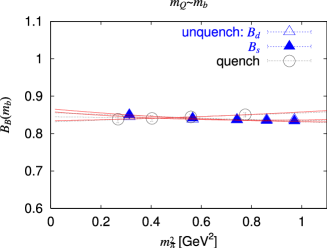
Figure 8: Dependence of $B_{B}$ and $B_{B_{s}}$ on light-quark (valence-quark) mass in $N_{f}=2$ ($N_{f}=0$) NRQCD [69]. The light-quark mass is parametrized by the mass squared of the pseudoscalar meson composed of quarks with that quark mass. The different curves correspond to linear (dotted) and quadratic (solid) fits.

There are many fewer calculations of $B_{B_{q}}$ than there are of $f_{B_{q}}$. However, the situation with chiral extrapolations and with unquenching appears to be much more favorable. Indeed, for $N_{f}=2$, the coefficient of the chiral logarithm for $B_{B}$ is in the range $-0.2<\frac{1}{2}(1-3g^{2})<0.4$ instead of $0.8<\frac{3}{4}(1+3g^{2})<1.9$ as it is for $f_{B}$, when $0.2<g<0.7$. For $g=0.6$, these coefficients are $0.0$ and $1.6$, respectively. This milder behavior is confirmed by the unquenched calculation of JLQCD [68, 69], whose results for the light-quark-mass dependence of $B_{B}$ and $B_{B_{s}}$ are shown in Fig. 8.  This mild light-quark-mass dependence is also observed in all quenched calculations [48, 47, 71, 72, 73] of which an example is shown in Fig. 8. Also evident from Fig. 8 is the fact the there is very little variation in going from $N_{f}=0$ to $N_{f}=2$, indicating that quenching effects are small for $B_{B}$ and $B_{B_{s}}$.

The situation is less clear when it comes to the heavy-quark-mass behavior of $B_{B_{q}}$. In [47, 48], $B$ parameters computed in the relativistic approach for heavy-quark masses around that of the charm are extrapolated up to the $b$, using HQET as a guide. Leading logs are accounted for in [48]. In [70], NLL corrections in the matching of QCD to HQET are included, and a calculation of $B_{B_{q}}$ in the static limit is used in conjunction with the relativistic results of [47] to reach the $b$-quark by interpolation. These three calculations indicate that $B_{B_{q}}$ increases with increasing $M_{B_{q}}$. On the other hand, the NRQCD results of [73], performed at quark masses above and around $m_{b}$, suggest an opposite behavior. This behavior is mild, however, and the different formulations agree at the physical $b$-quark mass. Moreover, once systematics errors are included, the significance of these inconsistencies becomes marginal.

The results of calculations of the NLO-RGI parameter, $\hat{B}^{\mbox{\tiny NLO}}_{B}$, are collected in Fig. 9, together with those for $B_{B_{s}}/B_{B}$. All methods give fully consistent results suggesting that residual systematic errors cancel in the ratio of matrix elements,

$$B_{B_{q}}=\frac{3}{8}\frac{\langle\bar{B}_{q}|(\bar{b}q)_{V-A}(\bar{b}q)_{V-A}|B_{q}\rangle}{\langle\bar{B}_{q}|\bar{q}\gamma^{\mu}\gamma_{5}b|0\rangle\langle 0|\bar{b}\gamma_{\mu}\gamma_{5}q|B_{q}\rangle}\ ,$$ (12)

used to define the $B$-parameters. This appears also to be true of quenching effects.

The mild dependence on light valence-quark mass further guarantees that errors on $B_{B_{s}}/B_{B}$ are small, of order 3%. The situation regarding the heavy-quark-mass dependence, however, should be clarified. This could be achieved by combining relativistic and HQET results obtained with non-perturbative renormalization in the continuum limit (see Sec. 2.3).

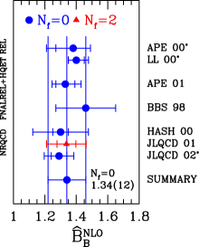
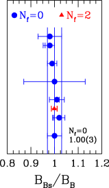
Figure 9: Lattice results for $\hat{B}^{\mbox{\tiny NLO}}_{B}$ and $B_{B_{s}}/B_{B}$. Calculations are grouped by the approach used for the heavy quark. The results shown are: APE 00 [47], LL 00 [48], APE 01 [70], BBS 98 [71], HASH 00 [72], JLQCD 01 [68], JLQCD 02 [73]. Also shown are my averages of the quenched results for these quantities.

4.3 $B_{q}-\bar{B}_{q}$–mixing: summary

I provide here summary numbers for the non-perturbative quantities relevant for the study of $B_{q}-\bar{B}_{q}$–mixing. In performing averages, I have only kept results dated after 1998 in the quenched case ($N_{f}=0$) and after 1999 for the unquenched case ($N_{f}=2$) and omit results which had not made it into proceedings or papers at the time of the conference. I use quenched averages as a starting point and the ratio of $N_{f}=2$ to $N_{f}=0$ results to extrapolate these results to $N_{f}=3$, including an additional systematic error equal to the shift from $N_{f}=2$ to $N_{f}=3$ in the final result. I obtain

$$f_{B}=203(27)^{+0}_{-20}\,\mathrm{Me\kern-1.00006ptV},\ f_{B_{s}}=238(31)\,\mathrm{Me\kern-1.00006ptV},$$ $$\hat{B}^{\mbox{\tiny NLO}}_{B}=1.34(12),\quad\hat{B}^{\mbox{\tiny NLO}}_{B_{s}}=1.34(12),$$ $$f_{B}\sqrt{\hat{B}^{\mbox{\tiny NLO}}_{B}}=235(33)^{+0}_{-24}\,\mathrm{Me\kern-1.00006ptV},$$ $$f_{B_{s}}\sqrt{\hat{B}^{\mbox{\tiny NLO}}_{B_{s}}}=276(38)\,\mathrm{Me\kern-1.00006ptV},$$

and

$$\frac{f_{B_{s}}}{f_{B}}=1.18(4)^{+12}_{-0},\quad\frac{B_{B_{s}}}{B_{B}}=1.00(3),$$ $$\xi\equiv\frac{f_{B_{s}}\sqrt{B_{B_{s}}}}{f_{B}\sqrt{B_{B}}}=1.18(4)^{+12}_{-0},$$

where the second, asymmetric error is the one due to the uncertainty in the chiral extrapolation of $f_{B}$ discussed above. This error should be viewed as rough estimate of the range of possible deviations that can be induced by including chiral logs in this extrapolation. Thus, in UT analyses, the value of $\xi$ given above should be understood as $\xi=1.24(4)(6)$  and similarly for the other quantities affected by this error. The results were not presented in this way because the inclusion of chiral logs is still exploratory. Note that this discussion does not concern $f_{B_{s}}$ and $f_{B_{s}}\sqrt{\hat{B}^{\mbox{\tiny NLO}}_{B_{s}}}$ whose residual chiral-log uncertainties appear to be small compared to other errors.

Before closing, let me mention that two groups have calculated $\xi$ directly from the ratio of $\Delta B=2$ matrix elements [71, 48]. The results obtained come out higher than the 1.18 given above, but are compatible within errors.

4.4 $K^{0}-\bar{K}^{0}$–mixing and $B_{K}$

The standard model, $\Delta S=2$ matrix element relevant for $CP$ violation in $K^{0}-\bar{K}^{0}$–mixing has been studied extensively on the lattice. A feature common to all but one of the calculations reviewed below is the use of the quenched approximation.  Furthermore, in these calculations, kaons are composed of mass-degenerate quarks and the final result is obtained by interpolation to a kaon of mass $M_{K}$, made up of two quarks of mass $\sim m_{s}/2$. The procedure has the advantage that a chiral extrapolation to the mass of the down quark is avoided. The drawback is that $SU(3)$-breaking corrections $\sim(m_{s}-m_{d})^{2}$ are not included and must be accounted for in the systematic error.

4.4.1 New calculations of $B_{K}$

This year three new quenched calculations of $B_{K}$ have been performed. The first, with Wilson type fermions, was presented at this conference [3, 75]. It is performed with high statistics at three different values of the lattice spacing in the range from $0.1$ to $0.06$ fermi, allowing for a continuum extrapolation. It implements a new method based on chiral Ward identities to eliminate the spurious mixing with wrong chirality four-quark operators [76] as well as the more traditional method of chiral subtractions. The authors find good agreement between their two preliminary results in the continuum limit. They renormalize the $B$-parameter non-perturbatively in the RI/MOM scheme.

The two other studies [77, 78] were performed using overlap quarks [79], a recent discretization of QCD which satisfies the Ginsparg-Wilson relation [80] and thus exhibits an exact chiral-flavor symmetry, analogous to the one of continuum QCD, at finite lattice spacing [81]. This symmetry implies that the $\Delta S=2$ operator is simple to construct on the lattice (unlike with staggered fermions) and does not mix with chirally dominant operators [82] (as it does with Wilson fermions). Overlap fermions further guarantee full $\mathcal{O}\left(a\right)$-improvement. These calculations are the first weak matrix element studies to use overlap quarks. They help validate this discretization as a useful phenomenological tool despite its present numerical cost. Such calculations will eventually verify that the explicit breaking of flavor (staggered fermions) or chiral (Wilson fermions) symmetry is controlled in standard calculations. They will also provide a check of domain wall fermion calculations. Domain wall quarks [83, 84] are a five-dimensional implementation of Ginsparg-Wilson fermions. The chiral-flavor symmetry which they exhibit becomes exact in the limit of infinite fifth dimension.

The first of these two overlap fermion calculations [77] is performed in the quenched approximation at a single value of the lattice spacing ($a^{-1}\sim 2\,\mathrm{Ge\kern-1.00006ptV}$) for five values of the light-quark mass in the range from $m_{s}/2$ to $1.3m_{s}$. The $B$-parameter is renormalized non-perturbatively in the RI/MOM scheme.

The second overlap calculation [78] is also performed in the quenched approximation, at two values of the lattice spacing ($a^{-1}\sim 1.7\,\mathrm{Ge\kern-1.00006ptV}$ and $2.2\,\mathrm{Ge\kern-1.00006ptV}$), with a slightly different action and with five light-quark masses, ranging from $0.8m_{s}$ to $2.5m_{s}$. In the mass interval common to both calculations, agreement is excellent. However, the large quark masses considered in [78] imply that the physical point is reached through a somewhat dangerous (linear) extrapolation. The resulting $B$-parameter is renormalized at one-loop. Results at the two lattice spacings are in good agreement.

Before summarizing the situation regarding $B_{K}$, I wish to mention that ALPHA [85] are performing a high-statistics calculation of this $B$-parameter using non-perturbative renormalization and a modified version of Wilson fermions which goes under the name of twisted-mass QCD [86]. This approach circumvents the problem of mixing with wrong chirality operators in much the same way as the Ward identity method of [76], which it inspired.

4.4.2 Summary of $B_{K}$ determinations

Results for $B^{\mbox{\tiny NDR}}_{K}(2\,\mathrm{Ge\kern-1.00006ptV})$ obtained by various groups using different approaches are plotted as a function of lattice spacing in Fig. 10. While results differ at finite lattice spacing, those which are extrapolated to the continuum limit agree in this limit within one-and-some standard deviations. The overlap results of [77, 78], obtained at finite lattice spacing, are also in good agreement with these continuum results, albeit with large statistical errors. Domain wall results are a bit on the low side. This difference should be understood through further scrutiny of systematic errors in those calculations.

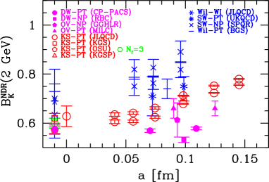
Figure 10: Lattice results for $B^{\mbox{\tiny NDR}}_{K}(2\,\mathrm{Ge\kern-1.00006ptV})$ vs lattice spacing. The results are coded according to the quark action used: Ginsparg-Wilson (filled symbols), staggered or Kogut-Susskind (unfilled symbols) and Wilson (stick symbols). The continuum limit corresponds to $a=0$. All but the reference result of JLQCD [89] in that limit are shifted to the left for clarity. The results shown are: CP-PACS [87], RBC [88], GGHLR [77], MILC [78], JLQCD (KS) [89], KGS [90], OSU and $N_{f}=3$ [91], KSGP [92], SPQR [75], JLQCD (Wilson) [93], UKQCD [94], BGS [95]. Not shown are the pioneering domain wall results of [96].

The reference result is still the one obtained in the 1997 quenched staggered calculation of JLQCD [89], which is the most complete study of this quantity to date, despite its use of one-loop perturbation theory in matching the lattice operators to their continuum counterparts. To their result one must add uncertainties due to quenching and the fact that the down and strange quarks are degenerate in the calculation. Sharpe [97], on the basis of quenched $\chi$PT and the preliminary “$N_{f}=3$” OSU results [91], suggests an enhancement factor of $1.05\pm 0.15$ to “unquench” quenched results for $B_{K}$. He advocates an additional factor $1.05\pm 0.05$ to compensate for the effect of working with degenerate quark masses. Here, I choose to keep his estimate of errors, but not to use his enhancement factors so as not to modify the central value on the basis of information which is provided by $\chi$PT estimates and preliminary lattice results. Thus, I quote

$$B^{\mbox{\tiny NDR}}_{K}(2\,\mathrm{Ge\kern-1.00006ptV})=0.628(42)(99)$$ $$\to\hat{B}^{\mbox{\tiny NLO}}_{K}=0.86(6)(14)\ ,$$

where $\hat{B}^{\mbox{\tiny NLO}}_{K}$ is the two-loop RGI $B$-parameter obtained from $B^{\mbox{\tiny NDR}}_{K}(2\,\mathrm{Ge\kern-1.00006ptV})$ with $N_{f}=3$ and $\alpha_{s}(2\,\mathrm{Ge\kern-1.00006ptV})=0.3$.

This is the same result as was presented at Lattice 2000 [7]. What is really needed now are high statistics unquenched calculations to reduce the dominant 15% quenching error. Without such an improvement in accuracy, indirect $CP$ violation in the neutral kaon system will no longer provide a significant constraint on UT fits [44].

4.5 Semileptonic decays

4.5.1 $|V_{cb}|$ from $B\to D^{*}\ell\nu$

The CKM element $|V_{cb}|$ plays an important r le in constraining the UT, for it determines the triangle’s base but also appears raised to the fourth power in the constraint on the summit provided by $\epsilon_{K}$. $|V_{cb}|$ must thus be determined as precisely as possible.

One way to measure $|V_{cb}|$ accurately is by extrapolating the differential decay rate for $B\to D^{*}\ell\nu$ decays,

$$\frac{d\Gamma}{dw}\sim|V_{cb}|^{2}\,|\mathcal{F}_{D^{*}}(w)|^{2}\ ,$$

to the zero-recoil point $w=v_{B}\cdot v_{D^{*}}=1$, where $v_{B}$ and $v_{D^{*}}$ are the four-velocities of the initial and final mesons [98]. The benefit of such an extrapolation is that heavy quark symmetry [99, 100] requires that the form factor $\mathcal{F}_{D^{*}}(w)$ must be normalized to 1 at $w=1$, up to small radiative and small order $1/m_{b,c}^{2}$ corrections [101]. Nevertheless, a few percent measurement of $|V_{cb}|$ requires a reliable determination of $\mathcal{F}_{D^{*}}(1)-1$. While the radiative corrections have been calculated to two-loops in perturbation theory [102], the long-distance power corrections require a non-perturbative treatment.

Through a clever use of double ratios of matrix elements for $D^{(*)},B^{(*)}\to D^{(*)},B^{(*)}$–like transitions, the authors of [103] have been able to obtain a statistically significant signal for the leading non-perturbative corrections of order $1/m_{b,c}^{2}$ and some of the sub-leading ones proportional to three factors of the inverse heavy-quark masses. The result of their quenched calculation, performed at three values of the lattice spacing, was presented at this conference [4, 103]:

$$\mathcal{F}_{D^{*}}(1)=0.913^{+24+17}_{-17-30}\ .$$

This important result, which requires excellent control of statistical and systematic errors, should be verified by other lattice groups.

4.6 $B\to\pi\ell\nu$ and $|V_{ub}|$

In heavy-to-light semileptonic decays, the light, final state hadron can have momenta as large as $|\vec{p}|\sim m_{Q}/2$ in the parent rest frame, where $m_{Q}$ is the mass of the heavy quark. For $m_{Q}=m_{b}$, and on present day lattices, such momenta would lead to uncontrollably large discretization effects, proportional to powers of $a|\vec{p}|$. Therefore, at present, only a limited kinematical range below the zero-recoil point can be reached without extrapolation. Even so, lattice calculations are useful, for the relevant matrix elements are not normalized by heavy quark symmetry as they are in $B\to D^{(*)}\ell\nu$ decays. Furthermore, experiment is beginning to measure the corresponding differential rates in the kinematical region accessible to lattice calculations (see e.g. [104]), thus allowing model-independent determinations of $|V_{ub}|$.

The matrix element relevant for $B^{0}\to\pi^{-}\ell^{+}\nu$ decays is

$$\langle\pi^{-}(p^{\prime})|V^{\mu}|B^{0}(p)\rangle=\frac{M_{B}^{2}-M_{\pi}^{2}}{q^{2}}q^{\mu}F_{0}(q^{2})$$

$$+(p+p^{\prime}-\frac{M_{B}^{2}-M_{\pi}^{2}}{q^{2}}q)^{\mu}F_{+}(q^{2})\ ,$$

where $q=p-p^{\prime}$ and $V^{\mu}=\bar{b}\gamma^{\mu}u$. There are four quenched calculations of this matrix element, using either relativistic, Fermilab or NRQCD heavy quarks. The form factors $F_{+}(q^{2})$ and $F_{0}(q^{2})$ obtained by the different collaborations are plotted as functions of $q^{2}$ in Fig. 11. Excellent agreement is found for $F_{+}(q^{2})$ which determines the rate in the limit of vanishing lepton mass. This agreement is certainly not trivial given the use of different heavy-quark approaches and the variations in the rather intricate analyses leading to the determination of these form factors. The error on this form factor is typically of order 20%.

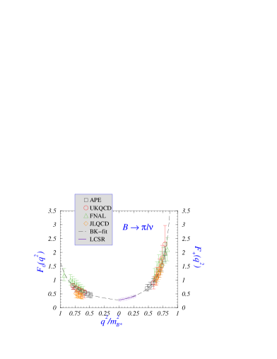
Figure 11: Lattice results for $B^{0}\to\pi^{-}\ell^{+}\nu$ form factors $F_{+}(q^{2})$ and $F_{0}(q^{2})$ (figure from [3]). These results are APE [105], UKQCD [106], FNAL [107], JLQCD [108]. Also shown is a fit to the parametrization of [109] and the light-cone sumrule results of [110] (see also [111]).

The lattice results cover roughly the upper half of the kinematically accessible range. The easiest way to extrapolate these results to lower values of $q^{2}$ is to use a parametrization such as the one presented in [109], which incorporates most of the known constraints on the form factors. Such an extrapolation is shown in Fig. 11 and gives excellent agreement with light-cone sumrule results [110, 111]. This extrapolation introduces, however, a model dependence. To eliminate this model dependence, one can make use of the dispersive bound techniques proposed in [112, 113]. In fact, the results of the analysis of [113] could certainly be improved with the lattice results presented here.

Given the good agreement amongst the different quenched calculations of $F_{+}(q^{2})$, what is needed to reduce the error on the extraction of $|V_{ub}|$ are unquenched calculations and more work on methods for enlarging the kinematical reach of lattice calculations.

5 Outlook

A number of quantities of central importance to particle physics are currently being studied with lattice QCD, many of which could unfortunately not be presented here. For those that were, emphasis is, in most cases, on the reduction of systematic errors, such as quenching, discretization errors, etc.

Because they have not yet led to phenomenological breakthroughs, I did not discuss in any detail the major advances of the last few years associated with the formulation and implementation of fermionic discretizations which preserve an exact continuum-like chiral-flavor symmetry at finite lattice spacing. These discretizations are known as Ginsparg-Wilson fermions [80], of which overlap [79], domain wall [83] and fixed-point fermions [114] are explicit realizations. They have opened new possibilities for the calculation of weak matrix elements, and in particular those associated with the $\Delta I=1/2$ rule and direct $CP$ violation in $K\to\pi\pi$ decays. On the analytical side, the renormalization of the weak operators involved has been studied with domain wall [115] and overlap fermions [116, 117]. On the numerical side, a first round of investigations has been performed with domain wall fermions [118, 88], laying the foundations for future studies.

The exceptional chiral properties of these new fermion formulations has also allowed the investigation of an unexplored regime of QCD in which the correlation length of the pion field is much larger than the linear extent of spacetime, the $\epsilon$-regime of [119]. This investigation has lead to exploratory calculations of one of the low-energy constants (LEC) of the strong chiral lagrangian in the quenched approximation [120, 121, 122, 123]. It is possible, in principle, to generalize this approach to extract the LECs of the weak chiral lagrangian and a numerical investigation is under way [124].

More generally, the range of approaches and of quantities studied in lattice QCD is constantly expanding and there should be many more exciting results to present at ICHEP 2004.

Acknowledgments

I thank D. Becirevic, C. Bernard, J. Charles, S. Collins, J. Flynn, L. Giusti, S. Hashimoto, V. Lubicz, G. Martinelli, F. Parodi, S. Sint, R. Sommer, A. Stocchi and N. Yamada for useful discussions and for their help in preparing this review. I would also like to thank the LOC, and Eric Laenen in particular, for their logistic support and more generally for making ICHEP 2002 a very interesting and enjoyable conference.

References

- [1] S. Collins, this volume.
- [2] H. Wittig, arXiv:hep-lat/0210025.
- [3] D. Becirevic, this volume.
- [4] J. Simone, this volume.
- [5] N. Ishizuka, arXiv:hep-lat/0209108.
- [6] C. T. Sachrajda, Int. J. Mod. Phys. A 17 (2002) 3140.
- [7] L. Lellouch, Nucl. Phys. PS 94 (2001) 142.
- [8] M. Alford, this volume.
- [9] S. Aoki et al. [CP-PACS Collaboration], arXiv:hep-lat/0206009.
- [10] C. Bernard et al., Nucl. Phys. PS 106 (2002) 412.
- [11] C. Bernard et al. [MILC Collaboration], arXiv:hep-lat/0209163.
- [12] C. Bernard et al., arXiv:hep-lat/0209086.
- [13] C. W. Bernard, Nucl. Phys. PS 94 (2001) 159.
- [14] S. M. Ryan, Nucl. Phys. PS 106 (2002) 86.
- [15] D. Becirevic, V. Lubicz and G. Martinelli, Phys. Lett. B 524 (2002) 115.
- [16] V. Gimenez, L. Giusti, F. Rapuano and M. Talevi, Nucl. Phys. B 540 (1999) 472.
- [17] K. G. Chetyrkin and A. Retey, Nucl. Phys. B 583 (2000) 3.
- [18] K. G. Chetyrkin, Phys. Lett. B 404 (1997) 161.
- [19] J. A. Vermaseren, S. A. Larin and T. van Ritbergen, Phys. Lett. B 405 (1997) 327.
- [20] J. Rolf and S. Sint [ALPHA Collaboration], arXiv:hep-ph/0209255.
- [21] S. Capitani et al. [ALPHA Collaboration], Nucl. Phys. B 544 (1999) 669.
- [22] R. Sommer, Nucl. Phys. B 411 (1994) 839.
- [23] A. S. Kronfeld, Nucl. Phys. PS 63 (1998) 311.
- [24] A. Bochkarev and Ph. de Forcrand, Nucl. Phys. B 477 (1996) 489; Nucl. Phys. PS 53 (1997) 305.
- [25] K. J. Juge, Nucl. Phys. PS 106 (2002) 847.
- [26] K. Hagiwara et al. [Particle Data Group Collaboration], Phys. Rev. D 66 (2002) 010001.
- [27] M. Crisafulli et al., Nucl. Phys. B 457 (1995) 594.
- [28] J. Heitger and R. Sommer [ALPHA collaboration], Nucl. Phys. PS 106 (2002) 358.
- [29] R. Sommer, arXiv:hep-lat/0209162.
- [30] F. Di Renzo and L. Scorzato, JHEP 0102 (2001) 020.
- [31] H. D. Trottier et al., Phys. Rev. D 65 (2002) 094502.
- [32] G. Martinelli and C. T. Sachrajda, Nucl. Phys. B 559 (1999) 429.
- [33] K. Melnikov and T. v. Ritbergen, Phys. Lett. B 482 (2000) 99.
- [34] M. Beneke and V. M. Braun, Nucl. Phys. B 426 (1994) 301.
- [35] I. I. Bigi et al., Phys. Rev. D 50 (1994) 2234.
- [36] C. T. Davies et al., Phys. Rev. Lett. 73 (1994) 2654.
- [37] K. Hornbostel [NRQCD Collaboration], Nucl. Phys. PS 73 (1999) 339.
- [38] A. Ali Khan et al., Phys. Rev. D 62 (2000) 054505.
- [39] V. Gimenez, G. Martinelli and C. T. Sachrajda, Nucl. Phys. B 486 (1997) 227.
- [40] V. Gimenez, L. Giusti, G. Martinelli and F. Rapuano, JHEP 0003 (2000) 018.
- [41] S. Collins, arXiv:hep-lat/0009040.
- [42] V. Lubicz, Nucl. Phys. PS 94 (2001) 116.
- [43] A. Stocchi, this volume.
- [44] F. Parodi, this volume and M. Ciuchini et al., JHEP 0107 (2001) 013.
- [45] A. H cker, H. Lacker, S. Laplace and F. Le Diberder, Eur. Phys. J. C 21 (2001) 225.
- [46] G. Buchalla, A. J. Buras and M. E. Lautenbacher, Rev. Mod. Phys. 68 (1996) 1125.
- [47] D. Becirevic et al., Nucl. Phys. B 618 (2001) 241.
- [48] L. Lellouch and C. J. Lin [UKQCD Collaboration], Phys. Rev. D 64 (2001) 094501.
- [49] K. C. Bowler et al. [UKQCD Collaboration], Nucl. Phys. B 619 (2001) 507.
- [50] A. X. El-Khadra et al., Phys. Rev. D 58 (1998) 014506.
- [51] A. Ali Khan et al. [CP-PACS Collaboration], Phys. Rev. D 64 (2001) 034505.
- [52] C. Bernard et al. [MILC Collaboration], arXiv:hep-lat/0206016.
- [53] A. Ali Khan et al., Phys. Lett. B 427 (1998) 132.
- [54] S. Collins et al., Phys. Rev. D 60 (1999) 074504.
- [55] A. Ali Khan et al. [CP-PACS Collaboration], Phys. Rev. D 64 (2001) 054504.
- [56] M. Guagnelli, F. Palombi, R. Petronzio and N. Tantalo, Phys. Lett. B 546 (2002) 237.
- [57] B. Grinstein et al., Nucl. Phys. B 380 (1992) 369.
- [58] S. R. Sharpe and Y. Zhang, Phys. Rev. D 53 (1996) 5125.
- [59] S. Ahmed et al. [CLEO Collaboration], Phys. Rev. Lett. 87 (2001) 251801.
- [60] A. Abada et al., arXiv:hep-lat/0209092.
- [61] P. Colangelo and F. De Fazio, Phys. Lett. B 532 (2002) 193.
- [62] P. Colangelo and A. Khodjamirian, arXiv:hep-ph/0010175.
- [63] D. Becirevic and A. L. Yaouanc, JHEP 9903 (1999) 021.
- [64] S. Hashimoto et al. [JLQCD Collaboration], arXiv:hep-lat/0209091.
- [65] N. Yamada, arXiv:hep-lat/0210035.
- [66] A. S. Kronfeld and S. M. Ryan, Phys. Lett. B 543 (2002) 59.
- [67] J. Gasser and H. Leutwyler, Annals Phys. 158 (1984) 142.
- [68] N. Yamada et al. [JLQCD Collaboration], Nucl. Phys. PS 106 (2002) 397.
- [69] N. Yamada for the JLQCD Collaboration, private communication.
- [70] D. Becirevic et al., JHEP 0204 (2002) 025.
- [71] C. W. Bernard, T. Blum and A. Soni, Phys. Rev. D 58 (1998) 014501.
- [72] S. Hashimoto et al., Phys. Rev. D 62 (2000) 114502.
- [73] S. Aoki et al. [JLQCD Collaboration], arXiv:hep-lat/0208038.
- [74] D. Becirevic et al., arXiv:hep-ph/0211271.
- [75] D. Becirevic et al. [SPQCDR Collaboration], arXiv:hep-lat/0209136.
- [76] D. Becirevic et al., Phys. Lett. B 487 (2000) 74.
- [77] N. Garron et al., CPT Marseille preprint CPT-2002/P.4416, september 2002.
- [78] T. DeGrand [MILC collaboration], arXiv:hep-lat/0208054.
- [79] H. Neuberger, Phys. Rev. D 57 (1998) 5417.
- [80] P. H. Ginsparg and K. G. Wilson, Phys. Rev. D 25 (1982) 2649.
- [81] M. L scher, Phys. Lett. B 428 (1998) 342.
- [82] P. Hasenfratz, Nucl. Phys. B 525 (1998) 401.
- [83] D. B. Kaplan, Phys. Lett. B 288 (1992) 342.
- [84] Y. Shamir, Nucl. Phys. B 406 (1993) 90.
- [85] M. Guagnelli et al. [ALPHA collaboration], arXiv:hep-lat/0209046.
- [86] R. Frezzotti et al. [ALPHA collaboration], JHEP 0108 (2001) 058.
- [87] A. Ali Khan et al. [CP-PACS Collaboration], Phys. Rev. D 64 (2001) 114506.
- [88] T. Blum et al. [RBC Collaboration], arXiv:hep-lat/0110075.
- [89] S. Aoki et al. [JLQCD Collaboration], Phys. Rev. Lett. 80 (1998) 5271.
- [90] G. Kilcup, R. Gupta and S. R. Sharpe, Phys. Rev. D57 (1998) 1654.
- [91] G. Kilcup, D. Pekurovsky and L. Venkataraman, Nucl. Phys. (PS) 53 (1997) 345.
- [92] G. Kilcup, S. R. Sharpe, R. Gupta and A. Patel, Phys. Rev. Lett. 64 (1990) 25.
- [93] S. Aoki et al. [JLQCD Collaboration], Phys. Rev. D60 (1999) 034511.
- [94] L. Lellouch and C. J. Lin [UKQCD Collaboration], Nucl. Phys. (PS) 73 (1999) 312.
- [95] R. Gupta, T. Bhattacharya and S. Sharpe, Phys. Rev. D55 (1997) 4036.
- [96] T. Blum and A. Soni, Phys. Rev. Lett. 79 (1997) 3595.
- [97] S. Sharpe, arXiv:hep-lat/9811006.
- [98] M. Neubert, Phys. Lett. B 264 (1991) 455.
- [99] M. A. Shifman and M. B. Voloshin, Sov. J. Nucl. Phys. 45, 292 (1987); 47, 511 (1988).
- [100] N. Isgur and M. B. Wise, Phys. Lett. B 232 (1989) 113; ibid. 237 (1990) 527.
- [101] M. E. Luke, Phys. Lett. B 252, 447 (1990).
- [102] A. Czarnecki, K. Melnikov and N. Uraltsev, Phys. Rev. D 57, 1769 (1998).
- [103] S. Hashimoto et al. Phys. Rev. D 66 (2002) 014503.
- [104] Y. Kwon, this volume.
- [105] A. Abada et al. Nucl. Phys. B 619 (2001) 565.
- [106] K. C. Bowler et al. [UKQCD Collaboration], Phys. Lett. B 486 (2000) 111.
- [107] A. X. El-Khadra et al. Phys. Rev. D 64 (2001) 014502.
- [108] S. Aoki et al. [JLQCD Collaboration], Phys. Rev. D 64 (2001) 114505.
- [109] D. Becirevic and A. B. Kaidalov, Phys. Lett. B 478 (2000) 417.
- [110] A. Khodjamirian et al., Phys. Rev. D 62 (2000) 114002.
- [111] P. Ball and R. Zwicky, JHEP 0110 (2001) 019.
- [112] C. G. Boyd, B. Grinstein and R. F. Lebed, Phys. Rev. Lett. 74 (1995) 4603.
- [113] L. Lellouch, Nucl. Phys. B 479 (1996) 353.
- [114] P. Hasenfratz, Nucl. Phys. Proc. Suppl. 63 (1998) 53.
- [115] S. Aoki and Y. Kuramashi, Phys. Rev. D 63 (2001) 054504.
- [116] S. Capitani and L. Giusti, Phys. Rev. D 64 (2001) 014506.
- [117] S. Capitani and L. Giusti, Phys. Rev. D 62 (2000) 114506.
- [118] J. I. Noaki et al. [CP-PACS Collaboration], arXiv:hep-lat/0108013.
- [119] J. Gasser and H. Leutwyler, Phys. Lett. B 188 (1987) 477.
- [120] P. Hern ndez, K. Jansen and L. Lellouch, Phys. Lett. B 469 (1999) 198.
- [121] P. Hern ndez, K. Jansen, L. Lellouch and H. Wittig, JHEP 0107 (2001) 018.
- [122] T. DeGrand [MILC Collaboration], Phys. Rev. D 64 (2001) 117501.
- [123] P. Hasenfratz et al., Nucl. Phys. B 643 (2002) 280.
- [124] L. Giusti et al., in preparation.