DESY 02-177
Edinburgh 2002/18
MPI-PhT/2002-70
PSI-PR-02-22
hep-ph/0211352

Abstract

The Higgs boson $\,H\,$ of the Standard Model can be searched for in the channels $\,p\bar{p}/pp\to t\bar{t}H+X\,$ at the Tevatron and the LHC. The cross sections for these processes and the final-state distributions of the Higgs boson and top quarks are presented at next-to-leading order QCD. To calculate these QCD corrections, a special calculational technique for pentagon diagrams has been developed and the dipole subtraction formalism has been adopted for massive particles. The impact of the corrections on the total cross sections is characterized by $K$ factors, the ratios of the cross sections in next-to-leading order over leading order QCD. At the central scale $\,\mu_{0}=(2m_{t}+M_{H})/2\,$ the $K$ factors are found to be slightly below unity for the Tevatron ($K\sim 0.8$) and slightly above unity for the LHC ($K\sim 1.2$). Including the corrections significantly stabilizes the theoretical predictions for total cross sections and for the distributions in rapidity and transverse momentum of the Higgs boson and top quarks.

November 2002

1 Introduction

Even though the Standard Model (SM) has been tremendously successful in describing matter and forces in particle physics, the third component of the model, the Higgs mechanism [1], has not been established yet experimentally. This component, however, is crucial for the closure of the SM in a mathematically consistent form, thereby allowing for systematic perturbative expansions and precise predictions in the electroweak sector [2]. The search for Higgs bosons [3, 4] is therefore one of the most important experimental programs in present-day high-energy physics [5].

For a light Higgs boson the electroweak interactions can be extended perturbatively up to the grand unification scale. The validity of this extrapolation is backed by the fact that it provides a qualitatively correct estimate of the electroweak mixing angle. Demanding, therefore, the perturbative extrapolation to hold up to the grand unification scale, the mass of the Higgs boson is bounded to be below 180 GeV in the SM [6]. An upper limit in the same range is also obtained experimentally by evaluating radiative corrections to electroweak precision observables, i.e. $M_{H}\leq 196$ GeV at the 95% confidence level [7]. A lower experimental mass limit of 114.4 GeV has been set by the LEP experiments [8].

In the near future, the search for Higgs bosons will continue at hadron colliders, the proton–antiproton collider Tevatron [3] with a centre-of-mass energy of 2 TeV, followed by the proton–proton collider LHC [4] with a centre-of-mass energy of 14 TeV. Various channels can be exploited at hadron colliders to search for Higgs bosons in the intermediate mass range. Among these channels, Higgs-boson radiation off heavy top quarks [9, 10, 11] plays an important rôle:

$$p\bar{p}/pp\to t\bar{t}H+X.$$ (1.1)

Although the expected rate is low at the Tevatron, a sample of a few but very clean events could be observed for Higgs masses below 140 GeV [12]. At the LHC, Higgs-boson radiation off the top quarks is an important search channel for Higgs masses below $\sim 125$ GeV [13, 14]. Moreover, analyzing the $t\bar{t}H$ production rate at the LHC can provide valuable information on the top–Higgs Yukawa coupling in relation to other Yukawa couplings [15, 16]. Precision measurements of the absolute value of the $t\bar{t}H$ coupling can be completed later at $e^{+}e^{-}$ colliders [17, 18, 19, 20, 21, 22].

Theoretical predictions for cross sections that are based merely on leading-order (LO) QCD are notoriously imprecise. They are plagued by considerable uncertainties owing to the strong dependence on the renormalization and factorization scales, introduced by the QCD coupling and the parton densities. Therefore, higher-order QCD corrections are needed for satisfactory theoretical predictions.

The cross sections for the processes (1.1) are found in next-to-leading order (NLO) QCD by convoluting the cross sections $d\sigma^{ab}$ of the parton subprocesses $ab\rightarrow t\bar{t}H(+k)$ with the parton distributions $f_{a}$ and $f_{b}$ of the initial-state hadrons, both evaluated in next-to-leading order:

$${\rm d}\sigma(h_{1}h_{2}\to t\bar{t}H+X)=\!\!\sum_{a,b=q,\bar{q},g}\int{\rm d}\xi_{a}\,f_{a}^{h_{1}}(\xi_{a};\mu_{\rm F}^{2})\int{\rm d}\xi_{b}\,f_{b}^{h_{2}}(\xi_{b};\mu_{\rm F}^{2})\;{\rm d}\sigma^{ab}(\hat{s}=\xi_{a}\xi_{b}s;\mu_{\rm F}^{2},\mu_{\rm R}^{2}).$$ (1.2)

In this convolution the partons $a$ and $b$ carry fractions $\xi_{a}$ and $\xi_{b}$ of the original momenta of the hadrons $h_{1}$ (= $p$) and $h_{2}$ (= $\bar{p}/p$), respectively. The total hadronic centre-of-mass energy is denoted by $\sqrt{s}$, whereas the partonic subprocess energy is given by $\sqrt{\hat{s}}$. The factorization and renormalization scales are denoted by $\mu_{F}$ and $\mu_{R}$, respectively. In general these two scales will be identified.

A brief report on the radiative QCD corrections for the processes (1.1) in NLO QCD has been presented for both the Tevatron and the LHC in Ref. [10]. The results of that study were found to be in agreement with a parallel investigation for the Tevatron in Ref. [11], which was based exclusively on the dominant partonic process $q\bar{q}\to t\bar{t}H$. As expected, in complete calculations of the NLO QCD corrections the scale dependence is reduced significantly, and stable theoretical predictions can be derived for the cross sections.

At the technical level there are two main obstacles in calculating the NLO QCD corrections. First, the one-loop pentagon (5-point) diagrams, involving both soft/collinear singularities and massive particles, have to be calculated in dimensional regularization. To this end, we have developed a calculational technique, exploiting the fact that the singularity structure of the pentagon diagrams can be derived in a universal way. This enables us to switch to regularization schemes that are more suitable for analyzing pentagon diagrams, without losing regularization-scheme-dependent constant terms. Second, the extraction of the singularities in the real part of the NLO QCD corrections has to be performed in a numerically stable way. For this purpose we have adopted the dipole subtraction formalism [23] for massive particles [24]. [This is the first application of this particular method to a complex NLO QCD calculation with massive quarks.] As an additional cross-check, the partial results for $q\bar{q}\to t\bar{t}H$ have been recalculated by means of the phase-space slicing method.

Besides the total cross sections, final-state distributions of the Higgs particle and the top quarks in rapidity $y$ and transverse momentum $p_{T}$ will be presented. As in the case of the total cross sections, including the NLO corrections significantly reduces the scale dependence of these distributions. It should be noted that based on this complete calculation, the NLO QCD corrections to arbitrary distributions can be investigated.

The report is divided into four sections. In the next section we describe the calculation of the NLO QCD corrections at the partonic level. In the third section the hadronic results for the SM reactions $p\bar{p}/pp\to t\bar{t}H$ are presented, comprising the total hadronic cross sections as well as the distributions in rapidity and transverse momentum. The analytical and numerical results of our study are summarized in the last section. Finally, the appendices provide some useful formulas, such as scalar one-loop integrals, results on colour algebra, and splitting functions.

2 Calculation of the NLO corrections

2.1 LO cross sections and conventions

The LO hadronic processes $p\bar{p}/pp\to t\bar{t}H+X$ proceed at the parton level via $q\bar{q}$ annihilation and $gg$ fusion:

$$q(p_{1})+\bar{q}(p_{2}) \to t(p_{3})+\bar{t}(p_{4})+H(p_{5}),$$ (2.1)

$$g(p_{1})+g(p_{2}) \to t(p_{3})+\bar{t}(p_{4})+H(p_{5}),$$ (2.2)

where the momenta of the particles are given in brackets. The momenta obey the on-shell conditions $p_{1}^{2}=p_{2}^{2}=0$, $p_{3}^{2}=p_{4}^{2}=m_{t}^{2}$, and $p_{5}^{2}=M_{H}^{2}$. For later use, the following set of kinematical invariants is defined:

$$\hat{s} = (p_{1}+p_{2})^{2},$$

$$s_{ij} = (p_{i}+p_{j})^{2},\qquad i,j=3,4,5,$$

$$t_{ij} = (p_{i}-p_{j})^{2},\qquad i=1,2,\quad j=3,4,5.$$ (2.3)

A generic set of LO diagrams is shown in Fig. 1; all LO diagrams not shown differ only in the point where the Higgs line is attached to the top-quark line.

Figure 1: The basic LO diagrams for the partonic processes $q\bar{q},gg\to t\bar{t}H$.

We express the amplitudes ${\cal{M}}^{q\bar{q},gg}$ of the LO and one-loop diagrams for the $q\bar{q}$ annihilation and the $gg$ fusion channel in terms of colour factors ${\cal C}^{q\bar{q},gg}_{j}$, standard matrix elements (SME) ${\cal{M}}^{q\bar{q},gg}_{i}$, and invariant functions $F^{q\bar{q},gg}_{ij}$. The SME include the Dirac structure, spinors, and polarization vectors in a standard form, while the $F^{q\bar{q},gg}_{ij}$ comprise all remaining factors, such as propagators, couplings, and standard one-loop integrals.

To introduce a compact notation for the SME, the tensors

$$\Gamma^{q\bar{q}}_{\{1,\mu,\mu\nu,\dots\}} = \bar{v}_{\bar{q}}(p_{2})\left\{{\bf 1},\gamma_{\mu},\gamma_{\mu}\gamma_{\nu},\dots\right\}u_{q}(p_{1}),$$

$$\Gamma^{t\bar{t}}_{\{1,\mu,\mu\nu,\dots\}} = \bar{u}_{t}(p_{3})\left\{{\bf 1},\gamma_{\mu},\gamma_{\mu}\gamma_{\nu},\dots\right\}v_{\bar{t}}(p_{4}),$$ (2.4)

are defined with obvious notations for the Dirac spinors $u_{q}(p_{1})$, etc. Furthermore, symbols like $\Gamma_{p}$ are used as shorthand for the contraction $\Gamma_{\mu}\,p^{\mu}$. For the $q\bar{q}$ channel we introduce the following set of SME,

$${\cal{M}}^{q\bar{q}}_{\{1,2,3,4\}} = \Gamma^{q\bar{q},\mu}\;\Gamma^{t\bar{t}}_{\{\mu,\mu p_{1},\mu p_{2},\mu p_{1}p_{2}\}},$$

$${\cal{M}}^{q\bar{q}}_{\{5,6,7,8\}} = \Gamma^{q\bar{q},\mu p_{3}p_{4}}\;\Gamma^{t\bar{t}}_{\{\mu,\mu p_{1},\mu p_{2},\mu p_{1}p_{2}\}},$$

$${\cal{M}}^{q\bar{q}}_{\{9,10,11,12\}} = \Gamma^{q\bar{q},p_{3}}\;\Gamma^{t\bar{t}}_{\{1,p_{1},p_{2},p_{1}p_{2}\}},$$

$${\cal{M}}^{q\bar{q}}_{\{13,14,15,16\}} = \Gamma^{q\bar{q},p_{4}}\;\Gamma^{t\bar{t}}_{\{1,p_{1},p_{2},p_{1}p_{2}\}},$$

$${\cal{M}}^{q\bar{q}}_{\{17,18,19,20\}} = \Gamma^{q\bar{q},\mu\nu p_{3}}\;\Gamma^{t\bar{t}}_{\{\mu\nu,\mu\nu p_{1},\mu\nu p_{2},\mu\nu p_{1}p_{2}\}},$$

$${\cal{M}}^{q\bar{q}}_{\{21,22,23,24\}} = \Gamma^{q\bar{q},\mu\nu p_{4}}\;\Gamma^{t\bar{t}}_{\{\mu\nu,\mu\nu p_{1},\mu\nu p_{2},\mu\nu p_{1}p_{2}\}},$$

$${\cal{M}}^{q\bar{q}}_{\{25,26,27,28\}} = \Gamma^{q\bar{q},\mu\nu\rho}\;\Gamma^{t\bar{t}}_{\{\mu\nu\rho,\mu\nu\rho p_{1},\mu\nu\rho p_{2},\mu\nu\rho p_{1}p_{2}\}}.$$ (2.5)

The LO amplitude ${\cal{M}}^{q\bar{q}}_{\mathrm{LO}}$ of the $q\bar{q}$ channel is proportional to the colour factor

$${\cal C}^{q\bar{q}}=\lambda^{c}\otimes\lambda^{c},$$ (2.6)

where the first Gell–Mann matrix $\lambda^{c}$ belongs to the $q\bar{q}$ state, the second matrix to the $t\bar{t}$ state. The one-loop amplitudes ${\cal{M}}^{q\bar{q}}_{{\mathrm{1-loop}}}$ also involve other colour operators, such as ${\bf 1}\otimes{\bf 1}$ and $(\lambda^{a}\lambda^{b})\otimes(\lambda^{a}\lambda^{b})$, but they can be reduced to multiples of ${\cal C}^{q\bar{q}}$ and tensors that are orthogonal to ${\cal C}^{q\bar{q}}$ and therefore do not contribute in the interference $\sum_{\mathrm{colours}}({\cal{M}}^{q\bar{q}}_{\mathrm{LO}})^{*}{\cal{M}}^{q\bar{q}}_{{\mathrm{1-loop}}}$. Thus, ${\cal C}^{q\bar{q}}$ is the only relevant colour structure at one loop, and the produced $t\bar{t}$ pair is in a pure colour-octet state in the $q\bar{q}$ channel. Both the LO and the (relevant part of the) one-loop amplitude can be written as

$${\cal{M}}^{q\bar{q}}={\cal C}^{q\bar{q}}{\cal A}^{q\bar{q}},\qquad{\cal A}^{q\bar{q}}=\sum_{i=1}^{28}F^{q\bar{q}}_{i}{\cal{M}}^{q\bar{q}}_{i},$$ (2.7)

leading in particular to

$$\sum_{\mathrm{spins,\,colours}}|{\cal{M}}^{q\bar{q}}_{\mathrm{LO}}|^{2}=32\sum_{\mathrm{spins}}|{\cal A}^{q\bar{q}}_{\mathrm{LO}}|^{2}.$$ (2.8)

Explicitly, the LO amplitude can be cast in the form

$${\cal{M}}^{q\bar{q}}_{\mathrm{LO}} = {}-{\cal C}^{q\bar{q}}\,\frac{\pi\alpha_{\mathrm{s}}g_{ttH}}{\hat{s}}\left[\phantom{+}\frac{1}{s_{35}-m_{t}^{2}}\left({\cal{M}}^{q\bar{q}}_{2}+{\cal{M}}^{q\bar{q}}_{3}+2{\cal{M}}^{q\bar{q}}_{13}\right)\right.$$ (2.9)

$$\left.\phantom{-{\cal C}^{q\bar{q}}\,\frac{\pi\alpha_{\mathrm{s}}g_{ttH}}{\hat{s}}\Bigg{\{}}{}+\frac{1}{s_{45}-m_{t}^{2}}\left({\cal{M}}^{q\bar{q}}_{2}+{\cal{M}}^{q\bar{q}}_{3}-2{\cal{M}}^{q\bar{q}}_{9}\right)\ \right],$$

from which the invariant functions $F^{q\bar{q}}_{\mathrm{LO},i}$ can be read off easily. The factor $g_{ttH}=m_{t}/v$ denotes the SM Yukawa coupling strength, where $v$ is the vacuum-expectation value of the Higgs field, and $\alpha_{\mathrm{s}}=g^{2}_{\mathrm{s}}/(4\pi)$ is the QCD coupling constant.

To define the SME for the $gg$ channel, the polarization vector $\varepsilon^{\mu}_{i}$ is introduced for each gluon with momentum $p^{\mu}_{i}$. Apart from the transversality condition $\varepsilon_{i}p_{i}=0$, the gauge conditions

$$\varepsilon_{1}p_{2}=\varepsilon_{2}p_{1}=0$$ (2.10)

are used to simplify the algebra in the calculation of the amplitudes. Within this gauge, the following set of SME is complete,

$${\cal{M}}^{gg}_{1} = \textstyle\frac{1}{4}\left[\Gamma^{t\bar{t}}_{p_{1}p_{2}\varepsilon_{1}\varepsilon_{2}}-\Gamma^{t\bar{t}}_{p_{2}p_{1}\varepsilon_{1}\varepsilon_{2}}-\Gamma^{t\bar{t}}_{p_{1}p_{2}\varepsilon_{2}\varepsilon_{1}}+\Gamma^{t\bar{t}}_{p_{2}p_{1}\varepsilon_{2}\varepsilon_{1}}\right],$$

$${\cal{M}}^{gg}_{\{2,3,4\}} = \Gamma^{t\bar{t}}_{1}\times\left\{(\varepsilon_{1}\varepsilon_{2}),(\varepsilon_{1}p_{3})(\varepsilon_{2}p_{3}),(\varepsilon_{1}p_{4})(\varepsilon_{2}p_{4})\right\},$$

$${\cal{M}}^{gg}_{5} = \textstyle\frac{1}{2}\left[\Gamma^{t\bar{t}}_{\varepsilon_{1}\varepsilon_{2}}-\Gamma^{t\bar{t}}_{\varepsilon_{2}\varepsilon_{1}}\right],$$

$${\cal{M}}^{gg}_{\{6,7,8\}} = \textstyle\frac{1}{2}\left[\Gamma^{t\bar{t}}_{p_{1}p_{2}}-\Gamma^{t\bar{t}}_{p_{2}p_{1}}\right]\times\left\{(\varepsilon_{1}\varepsilon_{2}),(\varepsilon_{1}p_{3})(\varepsilon_{2}p_{3}),(\varepsilon_{1}p_{4})(\varepsilon_{2}p_{4})\right\},$$

$${\cal{M}}^{gg}_{9} = \textstyle\frac{1}{2}\left[\Gamma^{t\bar{t}}_{p_{1}\varepsilon_{1}\varepsilon_{2}}-\Gamma^{t\bar{t}}_{p_{1}\varepsilon_{2}\varepsilon_{1}}\right],$$

$${\cal{M}}^{gg}_{\{10,11\}} = \textstyle\frac{1}{2}\left[\Gamma^{t\bar{t}}_{p_{1}p_{2}\varepsilon_{1}}-\Gamma^{t\bar{t}}_{p_{2}p_{1}\varepsilon_{1}}\right]\times\left\{(\varepsilon_{2}p_{3}),(\varepsilon_{2}p_{4})\right\},$$

$${\cal{M}}^{gg}_{\{12,13\}} = \Gamma^{t\bar{t}}_{p_{1}\varepsilon_{1}}\times\left\{(\varepsilon_{2}p_{3}),(\varepsilon_{2}p_{4})\right\},$$

$${\cal{M}}^{gg}_{\{14,15\}} = \Gamma^{t\bar{t}}_{p_{2}\varepsilon_{1}}\times\left\{(\varepsilon_{2}p_{3}),(\varepsilon_{2}p_{4})\right\},$$

$${\cal{M}}^{gg}_{16} = \textstyle\frac{1}{2}\left[\Gamma^{t\bar{t}}_{p_{1}p_{2}}-\Gamma^{t\bar{t}}_{p_{2}p_{1}}\right](\varepsilon_{1}p_{3})(\varepsilon_{2}p_{4}),$$

$${\cal{M}}^{gg}_{\{17,18\}} = \Gamma^{t\bar{t}}_{\varepsilon_{1}}\times\left\{(\varepsilon_{2}p_{3}),(\varepsilon_{2}p_{4})\right\},$$

$${\cal{M}}^{gg}_{\{19,20,21,22,23\}} = \Gamma^{t\bar{t}}_{p_{1}}\times\left\{(\varepsilon_{1}\varepsilon_{2}),(\varepsilon_{1}p_{3})(\varepsilon_{2}p_{3}),(\varepsilon_{1}p_{3})(\varepsilon_{2}p_{4}),(\varepsilon_{1}p_{4})(\varepsilon_{2}p_{3}),(\varepsilon_{1}p_{4})(\varepsilon_{2}p_{4})\right\},$$

$${\cal{M}}^{gg}_{24} = \Gamma^{t\bar{t}}_{1}(\varepsilon_{1}p_{3})(\varepsilon_{2}p_{4}),$$

$$\hat{\cal{M}}^{gg}_{i} = {\cal{M}}^{gg}_{i}\Big{|}_{p_{1}\leftrightarrow p_{2},\varepsilon_{1}\leftrightarrow\varepsilon_{2}},\qquad i=1,\dots,24.$$ (2.11)

In order to exhibit the Bose symmetry, the SME have been divided into the two subsets ${\cal{M}}^{gg}_{i}$ and $\hat{\cal{M}}^{gg}_{i}$ which transform into each other by interchanging the incoming gluons. Obviously the first eight SME of the two sets are Bose symmetric or antisymmetric,

$$\hat{\cal{M}}^{gg}_{i} = {}+{\cal{M}}^{gg}_{i},\qquad i=1,2,3,4,$$

$$\hat{\cal{M}}^{gg}_{i} = {}-{\cal{M}}^{gg}_{i},\qquad i=5,6,7,8.$$ (2.12)

Alternatively we may write

$${\cal{M}}^{gg}_{24+i}=\hat{\cal{M}}^{gg}_{8+i}={\cal{M}}^{gg}_{8+i}\Big{|}_{p_{1}\leftrightarrow p_{2},\varepsilon_{1}\leftrightarrow\varepsilon_{2}},\qquad i=1,\dots,16,$$ (2.13)

for the independent crossed SME $\hat{\cal{M}}^{gg}_{i}$ with $i>8$.

For the $gg$ channel it is convenient to introduce the three colour operators

$${\cal C}^{gg}_{1}=\delta^{c_{1}c_{2}}{\bf 1},\qquad{\cal C}^{gg}_{2}={\mathrm{i}}f^{c_{1}c_{2}c}\lambda^{c},\qquad{\cal C}^{gg}_{3}=d^{c_{1}c_{2}c}\lambda^{c},$$ (2.14)

where $c_{n}$ is the colour index of gluon $n$, and the matrices ${\bf 1}$ and $\lambda^{c}$ act on the $t\bar{t}$ state. The totally antisymmetric and symmetric SU(3) structure constants $f^{abc}$ and $d^{abc}$ are defined in the usual form. Parts in amplitudes that are proportional to different ${\cal C}^{gg}_{j}$ do not interfere with each other owing to the orthogonality relations:

$${\mathrm{Tr}}\left({\cal C}^{gg\dagger}_{j}{\cal C}^{gg}_{k}\right)=c^{gg}_{j}\delta_{jk}\qquad\mbox{with}\quad c^{gg}_{1}=24,\quad c^{gg}_{2}=48,\quad c^{gg}_{3}=\frac{80}{3}.$$ (2.15)

Obviously ${\cal C}^{gg}_{1}$ corresponds to a colour-singlet state of the $t\bar{t}$ system, while ${\cal C}^{gg}_{2}$ and ${\cal C}^{gg}_{3}$ describe the two different octet states. Both the LO and the one-loop amplitude can be written as

$${\cal{M}}^{gg}=\sum_{j=1}^{3}{\cal C}^{gg}_{j}{\cal A}^{gg}_{j},\qquad{\cal A}^{gg}_{j}=\sum_{i=1}^{40}F^{gg}_{ij}{\cal{M}}^{gg}_{i},$$ (2.16)

leading in particular to

$$\sum_{\mathrm{spins,\,colours}}|{\cal{M}}^{gg}_{\mathrm{LO}}|^{2}=\sum_{j=1}^{3}c^{gg}_{j}\sum_{\mathrm{spins}}|{\cal A}^{gg}_{\mathrm{LO},j}|^{2}.$$ (2.17)

Explicitly, the LO amplitude reads

$${\cal{M}}^{gg}_{\mathrm{LO}} = \phantom{{}+{}}\left(\frac{2}{3}{\cal C}^{gg}_{1}+{\cal C}^{gg}_{2}+{\cal C}^{gg}_{3}\right)\left(M_{\mathrm{direct}}+\frac{1}{2}M_{\mathrm{fusion}}\right)$$ (2.18)

$${}+\left(\frac{2}{3}{\cal C}^{gg}_{1}-{\cal C}^{gg}_{2}+{\cal C}^{gg}_{3}\right)\left(M_{\mathrm{crossed}}-\frac{1}{2}M_{\mathrm{fusion}}\right)$$

with

$$M_{\mathrm{direct}} = \frac{\pi\alpha_{\mathrm{s}}g_{ttH}}{(s_{45}-m_{t}^{2})(t_{13}-m_{t}^{2})}\biggl{[}{\cal{M}}^{gg}_{1}+\left(\frac{\hat{s}}{2}+t_{13}-m_{t}^{2}\right)({\cal{M}}^{gg}_{2}+{\cal{M}}^{gg}_{5})$$

$$\hphantom{\frac{\pi\alpha_{\mathrm{s}}g_{ttH}}{(s_{45}-m_{t}^{2})(t_{13}-m_{t}^{2})}\biggl{[}}{}-4{\cal{M}}^{gg}_{3}+{\cal{M}}^{gg}_{6}-2{\cal{M}}^{gg}_{12}-2\hat{\cal{M}}^{gg}_{12}\biggr{]}$$

$${}+\frac{\pi\alpha_{\mathrm{s}}g_{ttH}}{(t_{13}-m_{t}^{2})(t_{24}-m_{t}^{2})}\biggl{[}{\cal{M}}^{gg}_{1}+\frac{\hat{s}}{2}({\cal{M}}^{gg}_{2}+{\cal{M}}^{gg}_{5})+{\cal{M}}^{gg}_{6}+2{\cal{M}}^{gg}_{13}$$

$$\hphantom{{}+\frac{\pi\alpha_{\mathrm{s}}g_{ttH}}{(t_{13}-m_{t}^{2})(t_{24}-m_{t}^{2})}\biggl{[}}{}+4{\cal{M}}^{gg}_{24}-2\hat{\cal{M}}^{gg}_{12}\biggr{]}$$

$${}+\frac{\pi\alpha_{\mathrm{s}}g_{ttH}}{(s_{35}-m_{t}^{2})(t_{24}-m_{t}^{2})}\biggl{[}{\cal{M}}^{gg}_{1}+\left(\frac{\hat{s}}{2}+t_{24}-m_{t}^{2}\right)({\cal{M}}^{gg}_{2}+{\cal{M}}^{gg}_{5})$$

$$\hphantom{{}+\frac{\pi\alpha_{\mathrm{s}}g_{ttH}}{(s_{35}-m_{t}^{2})(t_{24}-m_{t}^{2})}\biggl{[}}{}-4{\cal{M}}^{gg}_{4}+{\cal{M}}^{gg}_{6}+2{\cal{M}}^{gg}_{13}+2\hat{\cal{M}}^{gg}_{13}\biggr{]},$$

$$M_{\mathrm{crossed}} = M_{\mathrm{direct}}\Big{|}_{t_{1i}\leftrightarrow t_{2i},\,{\cal{M}}^{gg}_{i}\leftrightarrow\hat{\cal{M}}^{gg}_{i}}\ ,$$

$$M_{\mathrm{fusion}} = \frac{2\pi\alpha_{\mathrm{s}}g_{ttH}}{\hat{s}(s_{45}-m_{t}^{2})}\biggl{[}(t_{13}-t_{23}){\cal{M}}^{gg}_{2}+2{\cal{M}}^{gg}_{6}\biggr{]}$$ (2.19)

$${}+\frac{2\pi\alpha_{\mathrm{s}}g_{ttH}}{\hat{s}(s_{35}-m_{t}^{2})}\biggl{[}(t_{24}-t_{14}){\cal{M}}^{gg}_{2}+2{\cal{M}}^{gg}_{6}\biggr{]}\ =\ -\,M_{\mathrm{fusion}}\Big{|}_{t_{1i}\leftrightarrow t_{2i},\,{\cal{M}}^{gg}_{i}\leftrightarrow\hat{\cal{M}}^{gg}_{i}}\ .\qquad\qquad$$

The terms in Eq. (2.18) proportional to $M_{\mathrm{direct}}$ correspond to the three “direct graphs”, where two parallel gluons couple to the top-quark line (see 3rd graph in Fig. 1). The terms proportional to $M_{\mathrm{crossed}}$ result from the direct graphs by crossing, i.e. by interchanging the two gluons (see 4th graph in Fig. 1). The terms proportional to $M_{\mathrm{fusion}}$ correspond to the gluon-fusion graphs (see 2nd graph in Fig. 1) which do not receive crossed counterparts.

Some comments on the SME and their evaluation ought to be added. The ${\cal{M}}^{q\bar{q},gg}_{i}$ defined above lead to a unique representation of all LO and one-loop diagrams, as indicated in Eqs. (2.7) and (2.16), if only the Dirac equation, the transversality of the polarization vectors, and the gauge conditions (2.10) are used. The number of SME could actually be reduced further by exploiting discrete symmetries and by using the four-dimensionality of space-time, inducing relations among the SME given above. However, eliminating some of the SME does not simplify the numerical evaluation significantly. The explicit calculation of the SME was carried out in two different ways. First all interference terms $\sum_{\mathrm{spins}}({\cal{M}}^{q\bar{q},gg}_{i})^{*}{\cal{M}}^{q\bar{q},gg}_{k}$ were calculated by making use of the general polarization sums for Dirac spinors and polarization vectors. In a second independent approach we directly expressed the ${\cal{M}}^{q\bar{q},gg}_{i}$ in terms of Weyl–van der Waerden spinor products [25] for each helicity configuration.

The final step in the calculation of the partonic cross sections and distributions involves the 4-dimensional integration over the final-state three-particle phase space. By introducing an intermediate “$t\bar{t}$-state” with virtuality $s_{34}$, one obtains

$${\mathrm{d}}\sigma_{\mathrm{LO}}^{ab} = \frac{1}{2\hat{s}}\,k^{ab}_{\mathrm{av}}\,\frac{1}{(2\pi)^{4}}\,\frac{\kappa(s_{34},m_{t}^{2},m_{t}^{2})}{8\,s_{34}}\,\frac{\kappa(\hat{s},s_{34},M_{H}^{2})}{8\,\hat{s}}\,\Theta(\sqrt{\hat{s}}-2m_{t}-M_{H})\,\Theta(s_{34}-4m_{t}^{2})\times$$ (2.20)

$$\times\,\Theta([\sqrt{\hat{s}}-M_{H}]^{2}-s_{34})\!\sum_{\mathrm{spins,\,colours}}|{\cal{M}}^{ab}_{\mathrm{LO}}|^{2}\,\,{\mathrm{d}}s_{34}\,\,{\mathrm{d}}\Omega_{t}^{*}\,\,{\mathrm{d}}\cos(\theta_{H}^{\mathrm{CM}})\,,$$

with

$$\kappa(x,y,z)=\sqrt{x^{2}+y^{2}+z^{2}-2xy-2xz-2yz}\,.$$ (2.21)

The labels $ab$ indicate the specific initial state of the partonic process. The solid angle $\Omega_{t}^{*}$ of the top quark is defined in the rest frame of the “$t\bar{t}$-state”, using the direction of flight of the “$t\bar{t}$-state” in the initial-state centre-of-mass frame as $z$-axis. The angle $\theta_{H}^{\mathrm{CM}}$ denotes the polar angle of the Higgs boson in the initial-state centre-of-mass frame, using the direction of the initial-state beams as $z$-axis. The corresponding azimuthal angle is trivially integrated to $2\pi$ in view of rotational invariance about the initial-state beams. The factor $k^{ab}_{\mathrm{av}}$ results from the average over the initial-state spins and colours:

$$k_{\mathrm{av}}^{q\bar{q}}=\frac{1}{36},\qquad k_{\mathrm{av}}^{gg}=\frac{1}{256},\qquad k_{\mathrm{av}}^{qg}=k_{\mathrm{av}}^{g\bar{q}}=\frac{1}{96}\,,$$ (2.22)

where $k_{\mathrm{av}}^{qg}$ and $k_{\mathrm{av}}^{g\bar{q}}$ are given for future use. The differential cross section including virtual NLO corrections can be obtained in a straightforward way from Eq. (2.20) by substituting the correct matrix element.

2.2 Virtual corrections

2.2.1 One-loop diagrams and calculational framework

Among the one-loop QCD diagrams, three different gauge-invariant subsets can be distinguished, for both the $q\bar{q}$ and $gg$ channels. Representative diagrams of these subsets are shown in Fig. 2.

Figure 2: Representative diagrams of the gauge-invariant subsets (i)-(iii) of one-loop QCD diagrams, as described in the text.

Subset (i) comprises all closed-quark-loop graphs where the Higgs boson couples to the external top-quark line, (ii) includes all graphs where the Higgs boson couples to a closed quark loop, and (iii) is formed by all other diagrams, which include at least one gluon in the loop. Counting closed quark loops only once per quark flavour, we get 2, 2, and 25 graphs of the respective subsets in the $q\bar{q}$ channel; and 6, 20, and 108 graphs in the $gg$ channel. The counting is performed in the Feynman gauge, omitting tadpole-like graphs and external self-energy corrections consistently. Of course, the subsets (i) and (iii) receive counterterm contributions from renormalization, which are considered in Section 2.2.2 in more detail; the second subset is not renormalized in NLO, since $Hgg$ and $Hggg$ couplings do not exist in LO.

In NLO the one-loop amplitudes ${\cal{M}}^{q\bar{q},gg}_{{\mathrm{1-loop}}}$ contribute via interference with the corresponding LO amplitudes ${\cal{M}}^{q\bar{q},gg}_{\mathrm{LO}}$. Using the colour decomposition rules of Section 2.1, the square of the sum of the LO amplitude and its virtual NLO correction reduces to

$$\sum_{\mathrm{spins,\,colours}}|{\cal{M}}^{q\bar{q}}_{\mathrm{LO}+({\mathrm{1-loop}})}|^{2} = 32\sum_{\mathrm{spins}}\left(|{\cal A}^{q\bar{q}}_{\mathrm{LO}}|^{2}+2\mathop{\mathrm{Re}}\nolimits\left\{({\cal A}^{q\bar{q}}_{\mathrm{LO}})^{*}{\cal A}^{q\bar{q}}_{{\mathrm{1-loop}}}\right\}\right),$$

$$\sum_{\mathrm{spins,\,colours}}|{\cal{M}}^{gg}_{\mathrm{LO}+({\mathrm{1-loop}})}|^{2} = \sum_{j=1}^{3}c^{gg}_{j}\sum_{\mathrm{spins}}\left(|{\cal A}^{gg}_{\mathrm{LO},j}|^{2}+2\mathop{\mathrm{Re}}\nolimits\left\{({\cal A}^{gg}_{\mathrm{LO},j})^{*}{\cal A}^{gg}_{{\mathrm{1-loop}},j}\right\}\right).$$ (2.23)

The evaluation of the virtual NLO correction was performed in two completely independent calculations, leading, in particular, to two independent computer codes. In the first evaluation, the Feynman graphs have been generated by using FeynArts [26]. These amplitudes have subsequently been reduced in terms of SME with the help of Mathematica. Following standard techniques of one-loop calculations [27, 28, 29, 30, 31], the tensor integrals are algebraically reduced to scalar integrals. The treatment of the so-called “pentagon” diagrams, involving five propagators in the loop, requires particular care and extensions of the standard methods given in Refs. [27, 28, 29, 30, 31]. The treatment of the pentagons is described in Section 2.2.3 in detail, where the results on the scalar 5-point functions are listed explicitly. The results on the divergent scalar 3- and 4-point functions are collected in Appendix A. Both ultraviolet (UV) and soft/collinear infrared (IR) divergences are treated in dimensional regularization. The renormalization, which removes the UV divergences, is discussed in Section 2.2.2. The explicit structure of the IR singularities occurring in the virtual corrections is given in Section 2.2.5, and the cancellation against their counterparts in the real corrections is described in Section 2.3. The algebraic output of the first calculation has been implemented in Fortran for numerical evaluation. The second calculation basically follows the same strategy, with a conceptual difference that is described in Section 2.2.3 (v). The amplitudes have been generated by hand and reduced with Form [32], and the numerical evaluation is carried out in C++.

For later use, we introduce the following definitions for the scalar and tensor integrals in analogy to Refs. [27, 28, 29, 30, 31],

$$B_{\{0,\mu,\mu\nu,\dots\}}(q_{1},m_{0},m_{1}) = \frac{(2\pi\mu)^{2\epsilon}}{{\mathrm{i}}\pi^{2}}\int{\mathrm{d}}^{D}q\,\frac{\{1,q_{\mu},q_{\mu}q_{\nu},\dots\}}{d_{0}d_{1}},$$

$$C_{\{0,\mu,\mu\nu,\dots\}}(q_{1},q_{2},m_{0},m_{1},m_{2}) = \frac{(2\pi\mu)^{2\epsilon}}{{\mathrm{i}}\pi^{2}}\int{\mathrm{d}}^{D}q\,\frac{\{1,q_{\mu},q_{\mu}q_{\nu},\dots\}}{d_{0}d_{1}d_{2}},$$

$$D_{\{0,\mu,\mu\nu,\dots\}}(q_{1},q_{2},q_{3},m_{0},m_{1},m_{2},m_{3}) = \frac{(2\pi\mu)^{2\epsilon}}{{\mathrm{i}}\pi^{2}}\int{\mathrm{d}}^{D}q\,\frac{\{1,q_{\mu},q_{\mu}q_{\nu},\dots\}}{d_{0}d_{1}d_{2}d_{3}},$$

$$E_{\{0,\mu,\mu\nu,\dots\}}(q_{1},q_{2},q_{3},q_{4},m_{0},m_{1},m_{2},m_{3},m_{4}) = \frac{(2\pi\mu)^{2\epsilon}}{{\mathrm{i}}\pi^{2}}\int{\mathrm{d}}^{D}q\,\frac{\{1,q_{\mu},q_{\mu}q_{\nu},\dots\}}{d_{0}d_{1}d_{2}d_{3}d_{4}},$$

$$\mbox{with}\quad d_{0}=q^{2}-m_{0}^{2}+{\mathrm{i}}0,\quad d_{j}=(q+q_{j})^{2}-m_{j}^{2}+{\mathrm{i}}0,\quad j=1,\dots,4.$$ (2.24)

Here $+{\mathrm{i}}0$ is the infinitesimal imaginary part as required by causality, $D=4-2\epsilon$ is the space-time dimension, and $\mu$ is the arbitrary reference scale of dimensional regularization, which we may identify with the renormalization scale. The UV and IR divergences appear as poles in $\epsilon$; it is convenient to use the abbreviations

$$\Delta_{1}(\mu) = \frac{\Gamma(1+\epsilon)}{\epsilon}\left(\frac{4\pi\mu^{2}}{m_{t}^{2}}\right)^{\epsilon},\qquad\Delta_{2}(\mu)=\frac{\Gamma(1+\epsilon)}{\epsilon^{2}}\left(\frac{4\pi\mu^{2}}{m_{t}^{2}}\right)^{\epsilon}$$ (2.25)

for these divergences. [The top-quark mass has been used to define a characteristic energy scale.] If we distinguish between UV and IR divergences, we explicitly write $\Delta^{\mathrm{UV},\mathrm{IR}}_{n}(\mu)$.

2.2.2 Renormalization

The renormalization is performed in the $\overline{\mathrm{MS}}$ scheme with the top-quark mass defined on shell. The top quark is decoupled from the running of the strong coupling $\alpha_{\mathrm{s}}(\mu)$. Denoting the bare top-quark mass and the bare strong coupling as $m_{t}^{0}$ and $\alpha_{\mathrm{s}}^{0}$, respectively, these conditions fix the renormalization parameters in the transformations $m_{t}^{0}=m_{t}+\delta m_{t}$ and $\alpha_{\mathrm{s}}^{0}=\alpha_{\mathrm{s}}+\delta\alpha_{\mathrm{s}}$ as follows,

$$\frac{\delta m_{t}}{m_{t}} = {}-\frac{\alpha_{\mathrm{s}}}{3\pi}\left[3\Delta^{\mathrm{UV}}_{1}(\mu)+4\right],$$

$$\frac{\delta\alpha_{\mathrm{s}}}{\alpha_{\mathrm{s}}} = \frac{\alpha_{\mathrm{s}}}{2\pi}\left(\frac{N_{f}}{3}-\frac{11}{2}\right)\Delta^{\mathrm{UV}}_{1}(m_{t})+\frac{\alpha_{\mathrm{s}}}{6\pi}\Delta^{\mathrm{UV}}_{1}(\mu),$$ (2.26)

where $N_{f}=5$ is the number of light flavours. The divergence $\Delta^{\mathrm{UV}}_{1}(m_{t})={\Gamma(1+\epsilon)}{(4\pi)^{\epsilon}}/{\epsilon}$ is independent of $\mu$ and originates from light-quark and gluon loops. The term proportional to $\Delta^{\mathrm{UV}}_{1}(\mu)$, on the other hand, originates from the top-quark loop in the gluon self-energy that is subtracted at zero-momentum transfer. In this scheme the running of the coupling $\alpha_{\mathrm{s}}(\mu)$ is generated solely by the finite contributions of the light-quark and gluon loops, while the top-quark contribution is absorbed completely in the renormalization condition and thus decouples effectively. The transformation for $m_{t}^{0}$ also fixes the renormalization of the Yukawa coupling, $g^{0}_{ttH}=m_{t}^{0}/v=(m_{t}+\delta m_{t})/v$, since $v$ does not receive NLO QCD corrections.

We renormalize the fields of the gluons, $G_{a,\mu}$, of the light quarks, $\psi_{q}$, and of the top quark, $\psi_{t}$, all in the on-shell scheme, i.e. the wave-function renormalization constants $\delta Z_{G,q,t}$, defined by the transformations

$$G_{a,\mu}^{0}=\left(1+\delta Z_{G}/2\right)G_{a,\mu},\qquad\psi_{q}^{0}=\left(1+\delta Z_{q}/2\right)\psi_{q},\qquad\psi_{t}^{0}=\left(1+\delta Z_{t}/2\right)\psi_{t},$$ (2.27)

are adjusted to cancel the external self-energy corrections exactly. Distinguishing between divergences of UV and IR origin, these constants can be written as

$$\delta Z_{G} = {}-\frac{\alpha_{\mathrm{s}}}{2\pi}\left(\frac{N_{f}}{3}-\frac{5}{2}\right)\left[\Delta^{\mathrm{UV}}_{1}(\mu)-\Delta^{\mathrm{IR}}_{1}(\mu)\right]-\frac{\alpha_{\mathrm{s}}}{6\pi}\Delta^{\mathrm{UV}}_{1}(\mu),$$

$$\delta Z_{q} = {}-\frac{\alpha_{\mathrm{s}}}{3\pi}\left[\Delta^{\mathrm{UV}}_{1}(\mu)-\Delta^{\mathrm{IR}}_{1}(\mu)\right],$$

$$\delta Z_{t} = {}-\frac{\alpha_{\mathrm{s}}}{3\pi}\left[\Delta^{\mathrm{UV}}_{1}(\mu)+2\Delta^{\mathrm{IR}}_{1}(\mu)+4\right].$$ (2.28)

The contributions of the counterterms and the external self-energies to the one-loop matrix elements ${\cal{M}}^{q\bar{q},gg}_{{\mathrm{1-loop}}}$ can be derived easily. For the $q\bar{q}$ channel they explicitly read

$${\cal{M}}_{\mathrm{ren}}^{q\bar{q}} = \left(\frac{\delta\alpha_{\mathrm{s}}}{\alpha_{\mathrm{s}}}+\frac{\delta m_{t}}{m_{t}}+\delta Z_{q}+\delta Z_{t}\right){\cal{M}}_{\mathrm{LO}}^{q\bar{q}}$$ (2.29)

$${}-{\cal C}^{q\bar{q}}\,\frac{\pi\alpha_{\mathrm{s}}g_{ttH}}{\hat{s}}\,\delta m_{t}\left[\phantom{+}\frac{2m_{t}}{(s_{35}-m_{t}^{2})^{2}}\left({\cal{M}}^{q\bar{q}}_{2}+{\cal{M}}^{q\bar{q}}_{3}+2{\cal{M}}^{q\bar{q}}_{13}\right)\right.$$

$$\left.\phantom{-{\cal C}^{q\bar{q}}\,\frac{\pi\alpha_{\mathrm{s}}g_{ttH}}{\hat{s}}\,\delta m_{t}\Biggl{[}}{}+\frac{2m_{t}}{(s_{45}-m_{t}^{2})^{2}}\left({\cal{M}}^{q\bar{q}}_{2}+{\cal{M}}^{q\bar{q}}_{3}-2{\cal{M}}^{q\bar{q}}_{9}\right)\right.$$

$$\left.\phantom{-{\cal C}^{q\bar{q}}\,\frac{\pi\alpha_{\mathrm{s}}g_{ttH}}{\hat{s}}\,\delta m_{t}\Biggl{[}}{}-\left(\frac{1}{s_{35}-m_{t}^{2}}+\frac{1}{s_{45}-m_{t}^{2}}\right){\cal{M}}^{q\bar{q}}_{1}\ \right].$$

The first term accounts for the external self-energy corrections as well as the counterterms of the strong and Yukawa coupling renormalization, while the remaining terms proportional to $\delta m_{t}$ come from the renormalization of the top-quark mass. For the $gg$ channel the former corrections have the same structure (proportional to the LO amplitude), but the mass renormalization involves cumbersome expressions.

2.2.3 Pentagon diagrams

(i) General strategy

Four different types of pentagon diagrams occur in the calculation; a representative of each type is shown in the last row of Fig. 2. Since the incoming quark $q$ is massless, three different types of 5-point functions are generated which involve one, two, or three massless propagators in the loop. Each of the three types is IR divergent, so that we need explicit results for scalar and tensor 5-point functions in $D\neq 4$ dimensions. As known for a long time [33], in $D=4$ dimensions all 5-point functions can be expressed in terms of 4-point functions, simplifying the calculation considerably. In the following we describe an elegant way how this reduction can be generalized for singular 5-point functions to $D\neq 4$ up to terms of order ${\cal O}(D-4)$ in dimensional regularization.

In order to make use of the reduction of 5-point functions to related 4-point functions, which works in four space-time dimensions, we first translate the dimensionally regularized integral $E^{(D)}$ into another regularization scheme that is defined in $D=4$ dimensions. To this end, we first endow all massless propagators in the loop with an infinitesimal mass $\lambda$ and call the new integral $E^{(\mathrm{mass},D)}$, which is identical to $E^{(D)}$ if $\lambda=0$. Next we determine a related well-defined integral, denoted $E^{(\mathrm{mass},D)}_{\mathrm{sing}}$, with the same IR (soft and collinear) singularity structure as $E^{(\mathrm{mass},D)}$. This integral is obtained by decomposing the integrand of the 5-point function in the collinear/soft limit in terms of 3-point integrands with regularization-scheme-independent kinematical prefactors [explicit examples are given below]. The difference of the two integrals, $E^{(\mathrm{mass},D)}-E^{(\mathrm{mass},D)}_{\mathrm{sing}}$, has a uniquely-determined finite integrand and is therefore regularization-scheme independent, i.e. the limits $D\to 4$ and $\lambda\to 0$ commute in this quantity. In total, we have generated in this way the relation

$$E^{(D)}-E^{(D)}_{\mathrm{sing}}+{\cal O}(D-4)=E^{(\mathrm{mass},D=4)}-E^{(\mathrm{mass},D=4)}_{\mathrm{sing}}+{\cal O}(\lambda).$$ (2.30)

If artificial UV divergences are introduced via $E^{(\mathrm{mass},D)}_{\mathrm{sing}}$ these divergences can be controlled by distinguishing the space-time dimensions $D_{\mathrm{IR}}$ and $D_{\mathrm{UV}}$ for the IR and UV domains explicitly. As shown below, the singular parts are given in terms of 3-point functions, and $E^{(\mathrm{mass},D=4)}$ can be expressed in terms of 4-point functions. Consequently, solving Eq. (2.30) for $E^{(D)}$,

$$E^{(D)}=E^{(D)}_{\mathrm{sing}}+\left[E^{(\mathrm{mass},D=4)}-E^{(\mathrm{mass},D=4)}_{\mathrm{sing}}\right]+\dots,$$ (2.31)

this integral is expressed (up to irrelevant terms indicated by the dots) in terms of 3-point and 4-point functions.

(ii) Determination of singular subintegrals in 5-point functions

Having described the general strategy, we now determine the singular terms in the relevant 5-point functions. The following derivation is valid for the integrals $E^{(\mathrm{mass},D)}$, which are defined for arbitrary $D$ in the vicinity of $D=4$ and which include infinitesimal mass regulators $\lambda$ for internal massless particles. The final formulae given for $E_{\mathrm{sing}}$ below are thus valid for both $E^{(D)}_{\mathrm{sing}}$ and $E^{(\mathrm{mass},D=4)}_{\mathrm{sing}}$. We do not write the regulator $\lambda$ explicitly, since the relations for $E_{\mathrm{sing}}$ also hold for other choices of mass regularizations.

We first consider the case of one vanishing internal mass, as shown in the second diagram of the last row in Fig. 2, for example. There is only a purely soft (logarithmic) divergence which is located at $q\to 0$ in the integrand if the vanishing mass is $m_{0}=0$. In this soft limit the numerator of the integral and the denominators $d_{2}$ and $d_{3}$ are regular. As a result, the singularity structure of the integral remains unchanged if we set $q=0$ in the numerator and the denominators $d_{2}$ and $d_{3}$, since the divergence is logarithmic. This, in particular, shows that all such tensor integrals $E_{\mu\dots}$ are finite, and only the scalar integral $E_{0}$ develops a soft singularity, which is already contained in a scalar 3-point function. There are two different types of 5-point integrals with one internal massless line, corresponding to the second diagram of the last row in Fig. 2 and the additional diagram generated by shifting the Higgs line along the top-quark line. Explicitly the singular parts of the corresponding integrals are given by

$$E_{0}(-p_{3},p_{1}-p_{3},p_{4}-p_{2},p_{4},0,m_{t},m_{t},m_{t},m_{t})_{\mathrm{sing}}$$

$$= \frac{1}{(t_{13}-m_{t}^{2})(t_{24}-m_{t}^{2})}\,C_{0}(-p_{3},p_{4},0,m_{t},m_{t}),$$

$$E_{0}(-p_{3},p_{1}-p_{3},p_{4}+p_{5},p_{4},0,m_{t},m_{t},m_{t},m_{t})_{\mathrm{sing}}$$ (2.32)

$$= \frac{1}{(t_{13}-m_{t}^{2})(s_{45}-m_{t}^{2})}\,C_{0}(-p_{3},p_{4},0,m_{t},m_{t}).$$

Next we consider the case with two internal massless lines, as generated, for example, in the third diagram of the last row in Fig. 2. In this case, the denominators $d_{i}$ are given by

$$d_{0} = q^{2},\qquad d_{1}=(q+p_{1})^{2},\qquad d_{2}=(q+p_{1}-p_{4})^{2}-m_{t}^{2},$$

$$d_{3} = (q+p_{3}-p_{2})^{2}-m_{t}^{2},\qquad d_{4}=(q+p_{3})^{2}-m_{t}^{2},$$ (2.33)

where the imaginary $i0$ terms are suppressed in the notation. The integral becomes singular in the collinear limit $q\to xp_{1}$ with arbitrary $x$, and in the soft limits $q\to 0$ and $q\to-p_{1}$, which are included in the collinear case for the limits $x\to 0$ and $x\to-1$, respectively. The non-singular denominators $d_{2,3,4}$ behave in the collinear limit as

$$d_{2} \sim (xp_{1}+p_{1}-p_{4})^{2}-m_{t}^{2}=(1+x)(t_{14}-m_{t}^{2}),$$

$$d_{3} \sim (xp_{1}+p_{3}-p_{2})^{2}-m_{t}^{2}={}-x(t_{13}-m_{t}^{2})-x\hat{s}+t_{23}-m_{t}^{2},$$

$$d_{4} \sim (xp_{1}+p_{3})^{2}-m_{t}^{2}={}-x(t_{13}-m_{t}^{2}),$$ (2.34)

and thus their inverse products as

$$\frac{1}{d_{2}d_{3}d_{4}} \sim \frac{1}{(s_{45}-m_{t}^{2})(t_{13}-m_{t}^{2})}\,\frac{1}{d_{2}}-\frac{(s_{45}-t_{23})^{2}}{(s_{45}-m_{t}^{2})(t_{13}-m_{t}^{2})(t_{14}-m_{t}^{2})(t_{23}-m_{t}^{2})}\,\frac{1}{d_{3}}$$ (2.35)

$${}+\frac{1}{(t_{14}-m_{t}^{2})(t_{23}-m_{t}^{2})}\,\frac{1}{d_{4}}.$$

This leads to the following decomposition of the singular part of the 5-point integral,

$$E_{\dots}(p_{1},p_{1}-p_{4},p_{3}-p_{2},p_{3},0,0,m_{t},m_{t},m_{t})_{\mathrm{sing}}$$ (2.36)

$$= \frac{1}{(s_{45}-m_{t}^{2})(t_{13}-m_{t}^{2})}\,C_{\dots}(p_{1},p_{1}-p_{4},0,0,m_{t})$$

$${}-\frac{(s_{45}-t_{23})^{2}}{(s_{45}-m_{t}^{2})(t_{13}-m_{t}^{2})(t_{14}-m_{t}^{2})(t_{23}-m_{t}^{2})}\,C_{\dots}(p_{1},p_{3}-p_{2},0,0,m_{t})$$

$${}+\frac{1}{(t_{14}-m_{t}^{2})(t_{23}-m_{t}^{2})}\,C_{\dots}(p_{1},p_{3},0,0,m_{t}).$$

This relation is valid for all tensors; in contrast to the case with only one vanishing mass, in this case also tensor integrals become singular. Note that $E_{\mathrm{sing}}$ does not only include the singularities but also regular terms in a well-defined way, which is important when switching from one regularization scheme to the other.

Finally, we consider the case with three internal masses zero, as encountered, e.g., in the first and last diagram of the last row in Fig. 2. Here three soft and two collinear limits give rise to divergences. Identifying $m_{0}=m_{1}=m_{4}=0$, the collinear limits are realized by setting $q\to xp_{1}\,$ or $\,q\to yp_{2}$, and the three soft limits are reached for particular values of $x$ and/or $y$ (i.e. $x=y=0$, $x=-1$, or $y=1$). The decomposition for the two collinear limits can be worked out in analogy to the previous case. When combining the two limits, however, double-counting of the soft singularity at $\,x=y=0\,$ has to be avoided. The decomposition of the singular structure of the 5-point integral finally reads

$$E_{\dots}(p_{1},p_{1}-p_{3},p_{4}-p_{2},-p_{2},0,0,m_{t},m_{t},0)_{\mathrm{sing}}$$ (2.37)

$$= \frac{1}{(t_{13}-m_{t}^{2})(t_{24}-m_{t}^{2})}\,C_{\dots}(p_{1},-p_{2},0,0,0)$$

$${}+\frac{1}{\hat{s}(s_{35}-m_{t}^{2})}\,C_{\dots}(p_{1},p_{1}-p_{3},0,0,m_{t})$$

$${}-\frac{(t_{24}-s_{35})^{2}}{\hat{s}(s_{35}-m_{t}^{2})(t_{13}-m_{t}^{2})(t_{24}-m_{t}^{2})}\,C_{\dots}(p_{1},p_{4}-p_{2},0,0,m_{t})$$

$${}+\frac{1}{\hat{s}(s_{45}-m_{t}^{2})}\,C_{\dots}(p_{4}-p_{2},-p_{2},0,m_{t},0)$$

$${}-\frac{(t_{13}-s_{45})^{2}}{\hat{s}(s_{45}-m_{t}^{2})(t_{13}-m_{t}^{2})(t_{24}-m_{t}^{2})}\,C_{\dots}(p_{1}-p_{3},-p_{2},0,m_{t},0),$$

which is again valid for all tensors.

(iii) The scalar 5-point function

In $D=4$ space-time dimensions the scalar 5-point function $E_{0}$ can be expressed [33] in terms of the five related 4-point functions $D_{0}(i)$, obtained from $E_{0}$ by omitting the denominator $d_{i}$, as defined in Eq. (2.24). Using the shorthand notations

$$Y_{00}=2m_{0}^{2},\quad Y_{i0}=Y_{0i}=m_{0}^{2}+m_{i}^{2}-q_{i}^{2},\quad Y_{ij}=m_{i}^{2}+m_{j}^{2}-(q_{i}-q_{j})^{2},\quad i,j=1,2,3,4,$$ (2.38)

the relation reads

$$0=\left|\begin{array}[]{cccccc}{}-E^{(\mathrm{mass},D=4)}_{0}&\>D^{(\dots)}_{0}(0)&\>D^{(\dots)}_{0}(1)&\>D^{(\dots)}_{0}(2)&\>D^{(\dots)}_{0}(3)&\>D^{(\dots)}_{0}(4)\\ 1&Y_{00}&Y_{01}&Y_{02}&Y_{03}&Y_{04}\\ 1&Y_{10}&Y_{11}&Y_{12}&Y_{13}&Y_{14}\\ 1&Y_{20}&Y_{21}&Y_{22}&Y_{23}&Y_{24}\\ 1&Y_{30}&Y_{31}&Y_{32}&Y_{33}&Y_{34}\\ 1&Y_{40}&Y_{41}&Y_{42}&Y_{43}&Y_{44}\end{array}\right|,$$ (2.39)

where the scalar integrals are defined for $D=4$. Solving for $E^{(\mathrm{mass},D=4)}_{0}$ we get

$$E^{(\mathrm{mass},D=4)}_{0}={}-\frac{1}{\det(Y)}\,\sum_{i=0}^{4}\,\det(Y_{i})\,D^{(\mathrm{mass},D=4)}_{0}(i),$$ (2.40)

where $Y=(Y_{ij})$, and $Y_{i}$ is obtained from $Y$ by replacing all entries in the $i$th column by 1.

Although Eq. (2.39) was derived for $D=4$, it is valid (in all cases considered here) even for arbitrary $D$ up to terms of order ${\cal O}(D-4)$:

$$E^{(D)}_{0}={}-\frac{1}{\det(Y)}\,\sum_{i=0}^{4}\,\det(Y_{i})\,D^{(D)}_{0}(i)+{\cal O}(D-4).$$ (2.41)

This generalized relation simply follows from the result derived in (ii) that the same linear relation between $E_{\mathrm{sing}}$ and 3-point subintegrals holds in all mass/dimensional regularization schemes.

(iv) Tensor 5-point functions

We evaluate all tensor integrals by calculating the coefficients to the Lorentz covariants that span the tensor. For the pentagons, tensor integrals $E_{\mu\nu\dots}$ appear up to rank 4. In practice, however, these integrals are needed only up to rank 3, since one momentum factor $q$ in the numerator of a top-quark propagator can always be cancelled against a propagator denominator. The covariant decomposition of the relevant 5-point tensor functions reads

$$E_{\mu} = \sum_{i=1}^{4}q_{i,\mu}E_{i},$$

$$E_{\mu\nu} = \sum_{i,j=1}^{4}q_{i,\mu}q_{j,\nu}E_{ij}+g_{\mu\nu}E_{00},$$

$$E_{\mu\nu\rho} = \sum_{i,j,k=1}^{4}q_{i,\mu}q_{j,\nu}q_{k,\rho}E_{ijk}+\sum_{i=1}^{4}\left(q_{i,\mu}g_{\nu\rho}+q_{i,\nu}g_{\mu\rho}+q_{i,\rho}g_{\mu\nu}\right)E_{00i}.$$ (2.42)

Since the tensors $E_{\mu\nu\dots}$ are symmetric, the tensor coefficients $E_{ij}$ and $E_{ijk}$ are symmetric in the indices. The coefficients $E_{i}$, $E_{ij}$, etc., can be recursively reduced to the scalar integrals $E_{0}$, $D_{0}$, etc., by an algorithm known as Passarino–Veltman reduction, as described in Refs. [28, 30], or by special techniques [34, 35] developed for higher $n$-point tensor integrals. The resulting expressions are cumbersome and do not reveal any new insight; therefore we do not list the expressions explicitly.

Note that the metric tensor appearing in Eq. (2.42) is $D$-dimensional. In contrast to the $D$-dimensional metric tensor $g_{\alpha\beta}$, its four-dimensional part, $g^{(D=4)}_{\alpha\beta}$, is spanned by the linearly independent base vectors $q_{i}$:

$$g^{(D=4)}_{\alpha\beta}=\sum_{i,j=1}^{4}\left(Z^{-1}\right)_{ij}q_{i,\alpha}q_{j,\beta},\qquad Z_{ij}=(q_{i}q_{j}),$$ (2.43)

where $Z$ is the Gram matrix of the momenta $q_{i}$. The difference $\Delta g_{\alpha\beta}=g_{\alpha\beta}-g^{(D=4)}_{\alpha\beta}$ is, thus, of ${\cal O}(D-4)$. It is interesting to notice that the terms proportional to $\Delta g_{\alpha\beta}$ do not contribute in our case. Since $\Delta g_{\alpha\beta}$ is an object of ${\cal O}(D-4)$ it could only contribute if an accompanying tensor coefficient, such as $E_{00}$, is divergent. The explicit tensor reduction to scalar integrals, however, reveals that all such coefficients are finite. This fact can also be derived from the following argument. In tensor integrals the only covariants that come with divergent coefficients are built up by the singular regions in momentum space. Therefore, a collinear divergence occurring for $q\to xp$ can only show up in tensors built up by the momentum $p$ alone. For purely soft (logarithmic) divergences occurring at $q\to 0$ power-counting shows that only the scalar integral is divergent; shifting the integration momentum by $p$, i.e. $q\to q+p$, only leads to divergent coefficients related to tensors of $p$ alone. UV divergences could occur in covariants containing $\Delta g_{\alpha\beta}$; however, all relevant 5-point integrals are UV-finite, which is easily proven by power-counting.

(v) Alternatives in practice

The results on 5-point functions described above admit two conceptually different ways to evaluate the pentagon diagrams. We followed both ways, as described below, and we found perfect numerical agreement.

In the first approach the scalar integral $E_{0}$ is evaluated in $D$ dimensions using Eq. (2.41) and also the reduction of the tensor coefficients defined in Eq. (2.42) is performed consistently in $D\neq 4$. In this approach all divergent scalar 3- and 4-point integrals $C_{0}$ and $D_{0}$ are needed in dimensional regularization. We have listed them in Appendix A.

Alternatively one can make consistent use of Eq. (2.31) and its analogous version for 4-point functions, in order to replace all $D$-dimensional 4- and 5-point integrals by four-dimensional integrals and $D$-dimensional 3-point functions that contain the IR (soft and collinear) singularities. The reduction of the 4- and 5-point tensor coefficients then works in four IR dimensions. An advantage of this procedure is the easy analytical control of all IR singularities which are contained in 3-point functions only. In this approach all divergent $D_{0}$ functions are needed in the mass-regularization scheme, and all divergent $C_{0}$ functions in both the dimensional and the mass-regularization schemes. The mass-regularized functions can be derived from the results of Appendix A. Another benefit of evaluating pentagon diagrams in four dimensions is the direct application of the tensor decomposition of Ref. [35]. This procedure consistently avoids leading Gram determinants (i.e. those of four momenta) that are potential sources of numerical instabilities, as described in the next section.

2.2.4 Numerical stabilization

As explained above, all tensor integrals occurring in the calculation can be algebraically reduced to scalar integrals following the well-known Passarino–Veltman algorithm [28]. This procedure is based on a decomposition of the tensor integral into a complete set of covariants that are spanned by the metric tensor and all independent momenta involved in the integral. The coefficients of the covariants are obtained by inverting a set of linear equations, which is non-singular as long as the momenta $q_{i}$ spanning the covariants are linearly independent, i.e. as long as their Gram determinant $G=\det(q_{i}q_{j})$ is non-zero. Each tensor rank adds a factor $G^{-1}$ to the expression of the tensor integral. Near the boundary of phase space, some determinants $G$ become arbitrarily small, since some momenta become linearly dependent at the boundary. The huge factors $G^{-n}$ are balanced by cancellations between different tensor coefficients that are calculated in terms of scalar integrals; the whole virtual correction remains well behaved at the phase-space boundary. These cancellations lead to severe numerical instabilities in the evaluation of the correction. The instabilities are most pronounced in the pentagon diagrams, which do not only possess the highest tensor ranks, but also involve additional sources of cancellations. For instance, the decomposition (2.43) of the four-dimensional metric tensor also leads to a Gram determinant in the denominator, and the reduction (2.39) of the scalar five-point function $E_{0}$ in terms of five four-point functions involves Caley determinants $\det(Y_{\dots})$ that can become very small.

If the virtual correction is not evaluated with particular care at the phase-space boundary, a phase-space point will soon be selected in the Monte Carlo integration where the result for the correction is totally wrong. The wrong result will typically be a large number owing to incomplete cancellations in the evaluation. Such unphysically large contributions occur more and more frequently in the adaptive integration procedure and they thus destroy the result of the phase-space integration completely .

When using the Passarino–Veltman procedure, we avoid the numerical instabilities by extrapolating the virtual correction from the numerically safe inner region of phase space to the numerically delicate boundary. To this end, we first divide the full phase space into two regions, one where the correction is evaluated directly and another where the correction is obtained from an extrapolation out of the first region.

The extrapolation procedure is applied to the full one-loop correction, since any subset of diagrams (such as the pentagons alone) in general shows stronger variations over the phase space than the full correction, owing to cancellations between different diagram types. Therefore, we have to inspect the whole boundary of phase space, which is characterized by the zero of the Gram determinant $G$ of the four momenta $p_{1},\dots,p_{4}$,

$$G=\frac{\hat{s}^{2}}{16}\,\kappa^{2}({\bf p}_{3}^{2},{\bf p}_{4}^{2},{\bf p}_{5}^{2})\,\sin^{2}\theta_{1}\,\sin^{2}\chi,$$ (2.44)

where $\kappa$ is defined in Eq. (2.21) and $p_{5}$ is fixed by momentum conservation, $p_{1}+p_{2}=p_{3}+p_{4}+p_{5}$. The three-momenta ${\bf p}_{i}$ and the angles $\theta_{1}$, $\chi$ are defined in the partonic centre-of-mass frame. The angle $\theta_{1}$ is the angle between ${\bf p}_{3}$ and the beam axis, and $\chi$ denotes the (azimuthal) angle between the ${\bf p}_{4}$–${\bf p}_{5}$ plane and the plane spanned by ${\bf p}_{3}$ and the beam axis. We identify the “safe” region by demanding $G/\hat{s}^{4}$ as well as $\sin\chi$ to be larger than certain numerical cut values. The extrapolation into the “problematic” region is done as follows:

1. Regarding the integrand as a function of the variable $\chi$, thereby keeping ${\bf p}_{3}$ and $|{\bf p}_{4}|$ fixed, we expand it in terms of a Fourier series. As a set of basis functions we took trigonometric functions or Legendre polynomials. The first few coefficients of the series are determined by numerical integration, for which we took Simpson or Gaussian quadrature. If the extrapolation result is close to the directly calculated result for the correction, the direct result is taken over.

2. If the agreement between direct and extrapolated result is too bad, the first step is repeated again with twice as many coefficients in the Fourier series and twice as many points in the related integration for the coefficients. The first step is repeated at most twice. If the directly calculated result is still not in good agreement with the extrapolation, but instead the various extrapolations look convergent, the most precise extrapolated result is taken over.

3. If the procedure still has not stopped yet, step one is modified by changing the extrapolation direction by varying also ${\bf p}_{3}$ and $|{\bf p}_{4}|$ during the change in $\chi$. Step two is carried out as above.

4. The modified extrapolation of step three is repeated if still no success has been reached. Finally, if none of the extrapolations looks convincing, the integration point is discarded, but this does not happen very often.

The extrapolation procedure solves the problem of numerical instabilities at the expense of computing time. Of course, the described procedure has to be optimized by selecting appropriate cut values on $G/\hat{s}^{4}$ and $\sin\chi$ and by choosing appropriate techniques for the calculation of the Fourier coefficients. Nevertheless the final phase-space integration has to be stable against any change in the extrapolation procedure. We have checked this stability by changing the cut parameters and by choosing different systems of orthogonal functions as well as different integration techniques, as mentioned above.

In addition to adopting the usual Passarino–Veltman reduction of 5-point tensor coefficients, we have applied the method of Ref. [35] where the strategy [33] for scalar 5-point functions is generalized and 5-point tensor coefficients are reduced to 4-point integrals directly. In this approach inverse Gram determinants of four momenta are avoided completely. Applying this alternative renders the virtual correction near the phase-space boundary much more stable than in the usual Passarino–Veltman approach. The results obtained by the two methods mutually agree with each other.

2.2.5 One-loop soft and collinear divergences

There are two sources of IR (soft and collinear) singularities in the one-loop diagrams: the self-energy corrections of the external fields and various kinds of 3-point subintegrals whenever a (nearly on-shell) gluon is exchanged between external lines. The former singularities can be read off from the results of Section 2.2.2, and the strategy to determine the latter singularities has already been explained in Section 2.2.3 (v). Here we list the explicit results:

$${\cal{M}}^{q\bar{q}}_{{\mathrm{1-loop}}}\Big{|}_{\mathrm{IR}} = \frac{\alpha_{\mathrm{s}}}{24\pi}\left(f^{q\bar{q}}_{12}-7f^{q\bar{q}}_{13}-2f^{q\bar{q}}_{23}-2f^{q\bar{q}}_{14}-7f^{q\bar{q}}_{24}+f^{q\bar{q}}_{34}\right){\cal{M}}^{q\bar{q}}_{\mathrm{LO}},$$ (2.45)

$${\cal{M}}^{gg}_{{\mathrm{1-loop}}}\Big{|}_{\mathrm{IR}} = {}-\frac{\alpha_{\mathrm{s}}}{24\pi}\Biggl{[}\left(9f^{gg}_{12}+9f^{gg}_{13}+9f^{gg}_{24}-f^{gg}_{34}\right)\left(\frac{2}{3}{\cal C}^{gg}_{1}+{\cal C}^{gg}_{2}+{\cal C}^{gg}_{3}\right)\left(M_{\mathrm{direct}}+\frac{1}{2}M_{\mathrm{fusion}}\right)$$ (2.46)

$$\quad{}+\left(9f^{gg}_{12}+9f^{gg}_{23}+9f^{gg}_{14}-f^{gg}_{34}\right)\left(\frac{2}{3}{\cal C}^{gg}_{1}-{\cal C}^{gg}_{2}+{\cal C}^{gg}_{3}\right)\left(M_{\mathrm{crossed}}-\frac{1}{2}M_{\mathrm{fusion}}\right)$$

$$\quad{}+6(f^{gg}_{12}-f^{gg}_{14}-f^{gg}_{23}+f^{gg}_{34})\,{\cal C}^{gg}_{1}\left(M_{\mathrm{direct}}+\frac{1}{2}M_{\mathrm{fusion}}\right)$$

$$\quad{}+6(f^{gg}_{12}-f^{gg}_{13}-f^{gg}_{24}+f^{gg}_{34})\,{\cal C}^{gg}_{1}\left(M_{\mathrm{crossed}}-\frac{1}{2}M_{\mathrm{fusion}}\right)\Biggr{]}.$$

The functions $M_{\dots}$ are given in Eq. (2.19), and the divergent factors $f^{q\bar{q}}_{ij}$ and $f^{gg}_{ij}$ read

$$f^{q\bar{q}}_{12} = 2\Delta^{\mathrm{IR}}_{2}(\mu)-2\Delta^{\mathrm{IR}}_{1}(\mu)\left[\ln\left({}-\frac{\hat{s}}{m_{t}^{2}}-{\mathrm{i}}0\right)-\frac{3}{2}\right],$$

$$f^{gg}_{12} = 2\Delta^{\mathrm{IR}}_{2}(\mu)-2\Delta^{\mathrm{IR}}_{1}(\mu)\left[\ln\left({}-\frac{\hat{s}}{m_{t}^{2}}-{\mathrm{i}}0\right)-\frac{11}{6}+\frac{N_{f}}{9}\right],$$

$$f^{q\bar{q}}_{ij} = \Delta^{\mathrm{IR}}_{2}(\mu)-\Delta^{\mathrm{IR}}_{1}(\mu)\left[2\ln\left(1-\frac{t_{ij}}{m_{t}^{2}}\right)-\frac{5}{2}\right],$$

$$f^{gg}_{ij} = \Delta^{\mathrm{IR}}_{2}(\mu)-\Delta^{\mathrm{IR}}_{1}(\mu)\left[2\ln\left(1-\frac{t_{ij}}{m_{t}^{2}}\right)-\frac{17}{6}+\frac{N_{f}}{9}\right],\qquad i=1,2,\quad j=3,4,$$

$$f^{q\bar{q}}_{34} = f^{gg}_{34}=2\Delta^{\mathrm{IR}}_{1}(\mu)\left[\frac{s_{34}-2m_{t}^{2}}{s_{34}\beta_{s_{34}}}\ln\left(\frac{\beta_{s_{34}}-1}{\beta_{s_{34}}+1}\right)+1\right],\qquad\beta_{s_{34}}=\sqrt{1-\frac{4m_{t}^{2}}{s_{34}}+{\mathrm{i}}0}\,.\hskip 20.00003pt$$ (2.47)

These results are in agreement with Ref. [36], where the general singularity structure of QCD amplitudes has been presented. The agreement becomes apparent after rewriting Eqs. (2.45) and (2.46) in the following generic form which is valid for both the $q\bar{q}$ and $gg$ channels,

$${\cal{M}}_{{\mathrm{1-loop}}}\Big{|}_{\mathrm{IR}}={\cal{M}}_{\mathrm{LO}}\otimes\frac{\alpha_{\mathrm{s}}}{4\pi}\sum_{i,j=1\atop i<j}^{4}({\bf T}_{i}\cdot{\bf T}_{j})\,f_{ij}.$$ (2.48)

Here ${\bf T}_{i}$ are the colour operators defined in Refs. [23, 24, 36], and the symbol $\otimes$ denotes the colour correlations. Since we will make repeated use of this notation in the remainder of our report, a short description can be found in Appendix B.

2.3 Real corrections

The real corrections at relative order ${\cal O}(\alpha_{\rm s})$ include processes with real-gluon radiation as well as $t\bar{t}H$ production in gluon-(anti)quark scattering. After a brief description of the parton reactions and their evaluation, we will discuss in some detail the isolation of IR divergences for soft and collinear parton configurations as well as the treatment of collinear initial-state singularities by means of mass factorization.

2.3.1 Parton processes and their evaluation

The evaluation of the ${\cal O}(\alpha_{\rm s}^{3}\,g_{ttH}^{2})$ cross section requires the calculation of the gluon bremsstrahlung processes

$$q(p_{1})+\bar{q}(p_{2}) \to t(p_{3})+\bar{t}(p_{4})+H(p_{5})+g(p_{6}),$$

$$g(p_{1})+g(p_{2}) \to t(p_{3})+\bar{t}(p_{4})+H(p_{5})+g(p_{6}),$$ (2.49)

and the gluon-(anti)quark scattering reactions

$$q(p_{1})+g(p_{2}) \to t(p_{3})+\bar{t}(p_{4})+H(p_{5})+q(p_{6}),$$

$$g(p_{1})+\bar{q}(p_{2}) \to t(p_{3})+\bar{t}(p_{4})+H(p_{5})+\bar{q}(p_{6}).$$ (2.50)

A representative set of Feynman diagrams, contributing to the real corrections, is given in Fig. 3.

Figure 3: Generic set of Feynman diagrams contributing to real gluon emission and gluon-(anti)quark scattering.

Helicity amplitudes for the processes (2.49, 2.50) have been generated and evaluated using the program packages MadGraph [37] and HELAS [38]. The result has been verified by an independent calculation based on standard trace techniques.

2.3.2 Soft and collinear divergences

The $2\to 4$ cross sections contain singularities in the limits where the splitting $g\to gg$, $g\to q\bar{q}$, $q\to qg$, or $\bar{q}\to\bar{q}g$ becomes soft or collinear. We have used the dipole subtraction method [23], as formulated in Ref. [24] for massive QCD partons, to extract the singular part of the real cross section in $D$ dimensions. The dipole subtraction method is based on the fact that soft and collinear limits of a real-emission matrix element can be expressed by convoluting process-independent splitting functions with the LO matrix element. By subtracting these splitting-function expressions as counterterms from the squared real matrix element, the IR (soft and collinear) singularities cancel and the phase-space integration can be performed numerically in four dimensions. The counterterms are constructed such that they can be integrated analytically in $D$ dimensions over the phase space of the extra emitted parton, leading to poles in $\epsilon=(4-D)/2$. When the integrated subtraction counterterms and the virtual cross sections are combined, the soft singularities cancel. The remaining initial-state collinear divergences have to be absorbed into a redefinition of the parton distribution functions at NLO. Below we will describe the subtraction formalism in more detail and we will give explicit results for the soft and collinear contributions.

The NLO contribution of the cross section can symbolically be written as [23, 24]

$$\sigma^{ab}_{\rm NLO}(p_{1},p_{2},\mu_{F}^{2}) = \sigma_{\rm NLO}^{ab\,\{4\}}(p_{1},p_{2})+\sigma_{\rm NLO}^{ab\,\{3\}}(p_{1},p_{2})$$ (2.51)

$${}+\int_{0}^{1}{\mathrm{d}}x\;\biggl{[}\hat{\sigma}_{\rm NLO}^{ab\,\{3\}}(x;xp_{1},p_{2},\mu_{F}^{2})+\hat{\sigma}_{\rm NLO}^{ab\,\{3\}}(x;p_{1},xp_{2},\mu_{F}^{2})\biggr{]}$$

$$= \int_{4}\biggl{\{}\Bigl{[}{\mathrm{d}}\sigma^{ab}_{\rm R}(p_{1},\dots,p_{6})\Bigr{]}_{\epsilon=0}\!-\biggl{[}\,\sum_{\mathrm{dipoles}}\!\!\Bigl{(}{\mathrm{d}}\sigma_{\rm LO}^{ab}\otimes\;{\mathrm{d}}V_{\mathrm{dipole}}\Bigr{)}(\tilde{p}_{1},\dots,\tilde{p}_{5},p_{6})\biggr{]}_{\epsilon=0}\,\biggr{\}}$$

$${}+\int_{3}\left[{\mathrm{d}}\sigma^{ab}_{\rm V}(p_{1},\dots,p_{5})+{\mathrm{d}}\sigma^{ab}_{\rm LO}(p_{1},\dots,p_{5})\otimes{\cal I}^{ab}\right]_{\epsilon=0}$$

$${}+\sum_{a^{\prime}=g,q,\bar{q}}\,\int_{0}^{1}{\mathrm{d}}x\int_{3}\left[{\mathrm{d}}\sigma_{\rm LO}^{a^{\prime}b}(xp_{1},p_{2},\tilde{p}_{3},\tilde{p}_{4},\tilde{p}_{5})\otimes\Gamma^{a,a^{\prime}}_{t\bar{t}H+b}(x,\mu_{F}^{2})\right]_{\epsilon=0}$$

$${}+\sum_{b^{\prime}=g,q,\bar{q}}\,\int_{0}^{1}{\mathrm{d}}x\int_{3}\left[{\mathrm{d}}\sigma_{\rm LO}^{ab^{\prime}}(p_{1},xp_{2},\tilde{p}_{3},\tilde{p}_{4},\tilde{p}_{5})\otimes\Gamma^{b,b^{\prime}}_{t\bar{t}H+a}(x,\mu_{F}^{2})\right]_{\epsilon=0}\;.$$

This symbolic expression is valid under the assumption that no massless particles are identified in the final state, i.e. the additional gluon or light (anti)quark is integrated out. The indices $a$ and $b$ denote the flavours of the incoming partons, i.e. $ab=q\bar{q},\,gg,\,qg,\,g\bar{q}$ in the processes (2.49,2.50), and $\mu_{F}$ is the factorization scale at which the redefinition of the parton distribution functions is performed at NLO. The notation for the integrals indicates that the real-emission contribution (labelled by $\rm R$) involves four final-state particles [one gluon or light (anti)quark more than in LO], while the virtual contribution (labelled by $\rm V$) has LO three-particle kinematics.

The dipole subtraction counterterm is given in terms of universal splitting functions, ${\mathrm{d}}V_{\mathrm{dipole}}$ (see Ref. [24] for explicit expressions), and an appropriate colour, spin, and flavour projection of the LO cross section, ${\mathrm{d}}\sigma_{\rm LO}$. The symbol $\otimes$ denotes such possible colour, spin, and flavour correlations. In particular, in the sum over “dipoles” the flavour correlations can change the incoming partons $a$ or $b$ in ${\mathrm{d}}\sigma_{\rm LO}^{ab}$. The final state of ${\mathrm{d}}\sigma_{\rm LO}$ is fixed to $t\bar{t}H$, since no light (anti)quark can be radiated from the top quarks. As far as the four-particle phase space is concerned, each individual dipole counterterm is evaluated for a specific set of auxiliary momenta $\tilde{p}_{1},\dots,\tilde{p}_{5}$. This involves combining the emitting particle (with momentum $p_{j}$) and the emitted light particle (with momentum $p_{6}$) into a single parent particle called “emitter” (with momentum $\tilde{p}_{j}$). In order to balance the total momentum, one of the other external particles (with momentum $p_{k}$) is replaced by a “spectator” particle (with the same quantum numbers, but modified momentum $\tilde{p}_{k}$). Apart from the situation where both emitter and spectator are incoming partons, the momenta of the remaining external particles are not altered. This phase-space mapping is constructed in such a way that

• the soft and (quasi-)collinear momentum configurations are reproduced point-wise;

• both the emitter and spectator are on their respective mass shells;

• momentum conservation is preserved;

• the phase space can be factorized into a hard-scattering phase space and a single-particle phase-space factor corresponding to $p_{6}$.

Many of these phase-space mappings either have an initial-state emitter or an initial-state spectator. In those cases the corresponding initial-state momentum is rescaled by a longitudinal momentum fraction $x$, resulting in a boosted reference frame for the final-state momenta and a phase-space factorization that involves a convolution over the boost parameter $x$. For explicit phase-space mappings we refer to the literature [23, 24].

The readded subtraction counterterm, integrated over the phase space of the emitted extra parton, can be split into two parts. The first part, involving the universal insertion operator ${\cal I}^{ab}$, has LO kinematics and contains all the poles in $\epsilon$ that are necessary to cancel the soft singularities in ${\mathrm{d}}\sigma^{ab}_{\rm V}$. These so-called endpoint contributions are obtained by integrating the dipoles over the complete phase space of the emitted extra parton and by using the $(\dots)_{+}$ prescription to extract the singular terms related to the soft endpoint ($x\to 1$) of the $x$-integration of the dipoles. The second part is a finite remainder that is left after factorization of initial-state collinear singularities into the parton distribution functions at NLO. It involves LO cross sections with boosted three-particle kinematics, $x$-dependent structure functions $\Gamma(x,\mu_{F}^{2})$, and an additional one-dimensional integration with respect to the longitudinal momentum fraction $x$ of an incoming parton. The structure functions $\Gamma(x,\mu_{F}^{2})$ depend on the factorization scheme; only the terms proportional to $\ln(\mu_{F}^{2})$ are factorization-scheme independent. The summations over the flavours $a^{\prime}$ and $b^{\prime}$ represent the afore-mentioned flavour correlations. Non-zero contributions are obtained if both ${\mathrm{d}}\sigma_{\rm LO}^{a^{\prime}b}$ and $\Gamma^{a,a^{\prime}}_{t\bar{t}H+b}$ are non-zero, or if both ${\mathrm{d}}\sigma_{\rm LO}^{ab^{\prime}}$ and $\Gamma^{b,b^{\prime}}_{t\bar{t}H+a}$ are non-zero.

In the remainder of this subsection we give the explicit expressions for the readded subtraction counterterms, which are based on the results of Ref. [24]. The explicit construction of the dipole terms, which is not described here, can also be found there. We start with the insertion operator ${\cal I}^{ab}$, which depends on the colour charges, momenta, and masses of the final-state particles in the LO matrix element:

$${\cal I}^{qg}={\cal I}^{g\bar{q}}=0,\qquad{\cal I}^{ab}=-\,\frac{\alpha_{\mathrm{s}}}{2\pi}\sum_{i,j=1\atop i<j}^{4}({\bf T}_{i}\cdot{\bf T}_{j})\,{\cal J}_{ij}^{ab},\qquad ab=q\bar{q},gg,$$ (2.52)

with

$${\cal J}_{12}^{ab} = 2\Delta^{\mathrm{IR}}_{2}(\mu)-2\Delta^{\mathrm{IR}}_{1}(\mu)\left[\ln\left(\frac{\hat{s}}{m_{t}^{2}}\right)-\frac{\gamma_{a}}{{\bf T}_{a}^{2}}\right]+\ln^{2}\left(\frac{\hat{s}}{m_{t}^{2}}\right)-2\,\frac{\gamma_{a}}{{\bf T}_{a}^{2}}\ln\left(\frac{\hat{s}}{m_{t}^{2}}\right)-\frac{2}{3}\,\pi^{2},$$

$${\cal J}_{34}^{ab} = 2\,\frac{s_{34}-2m_{t}^{2}}{s_{34}\beta_{s_{34}}}\Biggl{\{}\,\left[\Delta^{\mathrm{IR}}_{1}(\mu)-\ln\left(\frac{s_{34}}{m_{t}^{2}}\right)\right]\ln(\rho)-4\ln(\rho)\ln(1-\rho)-\frac{1}{2}\ln^{2}(\rho)$$

$${}-2\mathop{\mathrm{Li}_{2}}\nolimits(1-\rho^{2})-2\mathop{\mathrm{Li}_{2}}\nolimits(1-\rho)\,\Biggr{\}}$$

$${}+2\Delta^{\mathrm{IR}}_{1}(\mu)-2\ln\left(\frac{s_{34}}{m_{t}^{2}}\right)+6+\frac{2s_{34}}{s_{34}-2m_{t}^{2}}\ln\left(\frac{\sqrt{s_{34}}-m_{t}}{m_{t}}\right)$$

$${}-4\ln\left(\frac{\sqrt{s_{34}}-2m_{t}}{m_{t}}\right)-\frac{2m_{t}}{\sqrt{s_{34}}-m_{t}}-\frac{4m_{t}(\sqrt{s_{34}}-2m_{t})}{s_{34}-2m_{t}^{2}},$$

$${\cal J}_{ij}^{ab} = \Delta^{\mathrm{IR}}_{2}(\mu)-\Delta^{\mathrm{IR}}_{1}(\mu)\left[2\ln\left(1-\frac{t_{ij}}{m_{t}^{2}}\right)-\frac{\gamma_{a}}{{\bf T}_{a}^{2}}-1\right]+\frac{1}{2}\ln\left(2-\frac{t_{ij}}{m_{t}^{2}}\right)+\ln^{2}\left(1-\frac{t_{ij}}{m_{t}^{2}}\right)$$ (2.53)

$$-\left(\frac{\gamma_{a}}{{\bf T}_{a}^{2}}+2\right)\ln\left(1-\frac{t_{ij}}{m_{t}^{2}}\right)+\frac{3}{2}-\frac{2}{3}\,\pi^{2}-2\mathop{\mathrm{Li}_{2}}\nolimits\left(\frac{-\,1}{1-t_{ij}/m_{t}^{2}}\right)+\frac{1}{4-2\,t_{ij}/m_{t}^{2}},$$

$$\rm{for}\quad i=1,2\quad\rm{and}\quad j=3,4.$$

The variable $\beta_{s_{34}}$ is defined in Eq. (2.47) and $\rho$ is given by $\rho=(1-\beta_{s_{34}})/(1+\beta_{s_{34}})$. The dilogarithm $\mathop{\mathrm{Li}_{2}}\nolimits(x)$ is defined in the usual way as

$$\mathop{\mathrm{Li}_{2}}\nolimits(x)={}-\int_{0}^{1}{\mathrm{d}}t\,\frac{\ln(1-xt)}{t}.$$ (2.54)

The Casimir operators ${\bf T}_{a}^{2}$ and anomalous dimensions $\gamma_{a}$ read explicitly

$${\bf T}_{q}^{2}={\bf T}_{\bar{q}}^{2}\equiv C_{\mathrm{F}}=\frac{4}{3},\quad \quad\frac{\gamma_{q}}{{\bf T}_{q}^{2}}=\frac{\gamma_{\bar{q}}}{{\bf T}_{\bar{q}}^{2}}=\frac{3}{2},$$

$${\bf T}_{g}^{2}\equiv C_{\mathrm{A}}=3,\quad \quad\frac{\gamma_{g}}{{\bf T}_{g}^{2}}=\frac{11}{6}-\frac{N_{f}}{9}.$$ (2.55)

Inserting all this in Eq. (2.53), we observe indeed that the singular $\Delta^{\mathrm{IR}}_{2}(\mu)$ and $\Delta^{\mathrm{IR}}_{1}(\mu)$ terms in the functions ${\cal J}_{ij}^{ab}$ cancel against the singular terms in the coefficients $f_{ij}^{ab}$ given in Eq. (2.47).

Finally, we give a general expression for the structure function $\Gamma^{a,a^{\prime}}_{t\bar{t}H+b}(x,\mu_{F}^{2})$ in the $\overline{\mathrm{MS}}$ factorization scheme:

$$\Gamma^{a,a^{\prime}}_{t\bar{t}H+b} = \frac{\alpha_{\mathrm{s}}}{2\pi}\Biggl{\{}\ln\left(\frac{\hat{s}}{\mu_{F}^{2}}\right)P^{aa^{\prime}}(x)+2P_{\mathrm{reg}}^{aa^{\prime}}(x)\ln(1-x)+\hat{P}^{\prime}_{aa^{\prime}}(x)+4\,\delta^{aa^{\prime}}{\bf T}_{a}^{2}\left[\frac{\ln(1-x)}{1-x}\right]_{+}\Biggr{\}}$$ (2.56)

$$+ \frac{\alpha_{\mathrm{s}}}{2\pi}\sum_{j=3}^{4}\frac{({\bf T}_{a^{\prime}}\cdot{\bf T}_{j})}{{\bf T}_{a^{\prime}}^{2}}\Biggl{\{}\ln\left(\frac{\hat{s}\,\mu_{j1}^{2}}{m_{t}^{2}}\right)P^{aa^{\prime}}(x)+P_{\mathrm{reg}}^{aa^{\prime}}(x)\ln(1-x+\mu_{j1}^{2})$$

$$\hphantom{\frac{\alpha_{\mathrm{s}}}{2\pi}\sum_{j=3}^{4}\frac{({\bf T}_{a^{\prime}}\cdot{\bf T}_{j})}{{\bf T}_{a^{\prime}}^{2}}a}{}+2\,\delta^{aa^{\prime}}{\bf T}_{a}^{2}\left[\frac{1}{1-x}\,\Bigl{(}1+\ln[1-x+\mu_{j1}^{2}]\Bigr{)}-\frac{1-x}{4(1-x+\mu_{j1}^{2})^{2}}\right]_{+}$$

$$\hphantom{\frac{\alpha_{\mathrm{s}}}{2\pi}\sum_{j=3}^{4}\frac{({\bf T}_{a^{\prime}}\cdot{\bf T}_{j})}{{\bf T}_{a^{\prime}}^{2}}a}{}+2\,\delta^{ga^{\prime}}{\bf T}_{a}^{2}\,\frac{\mu_{j1}^{2}}{x}\ln\left(\frac{1-x+\mu_{j1}^{2}}{\mu_{j1}^{2}}\right)\Biggr{\}}.$$

The various Altarelli–Parisi splitting functions $P^{aa^{\prime}}(x)$, $P_{\mathrm{reg}}^{aa^{\prime}}(x)$, and $\hat{P}^{\prime}_{aa^{\prime}}(x)$ can be found in Appendix C, and the kinematical variable $\mu_{j1}^{2}$ is given by

$$\mu_{j1}^{2}=\frac{m_{t}^{2}}{2p_{1}\tilde{p}_{j}}\,,$$ (2.57)

where $\tilde{p}_{j}$ is the auxiliary momentum of particle $j$ in the boosted reference frame, while $p_{1}$ is the original initial-state momentum of the incoming parton $a$. In our convention the $(\dots)_{+}$ prescription is defined by

$$\int_{0}^{1}{\mathrm{d}}x\int{\mathrm{d}}\Phi(x)\,\Bigl{[}f(x,\mu^{(x)}_{j1})\Bigr{]}_{+}g(\Phi(x))$$ (2.58)

$$=\ \int_{0}^{1}{\mathrm{d}}x\int{\mathrm{d}}\Phi(x)\int_{-\infty}^{\infty}{\mathrm{d}}\bar{\mu}\,\,\delta(\bar{\mu}-\mu^{(x)}_{j1})\,\Bigl{[}f(x,\bar{\mu})\Bigr{]}_{+}g(\Phi(x))$$

$$=\ \int_{0}^{1}{\mathrm{d}}x\int_{-\infty}^{\infty}{\mathrm{d}}\bar{\mu}\,f(x,\bar{\mu})\,\biggl{\{}\,\int{\mathrm{d}}\Phi(x)\,g(\Phi(x))\,\delta(\bar{\mu}-\mu^{(x)}_{j1})$$

$$\hphantom{=\ \int_{0}^{1}{\mathrm{d}}x\int_{-\infty}^{\infty}{\mathrm{d}}\bar{\mu}\,f(x,\bar{\mu})a}{}-\int{\mathrm{d}}\Phi(1)\,g(\Phi(1))\,\delta(\bar{\mu}-\mu^{(1)}_{j1})\Biggr{\}}$$

$$=\ \int_{0}^{1}{\mathrm{d}}x\,\biggl{\{}\,\int{\mathrm{d}}\Phi(x)\,f(x,\mu^{(x)}_{j1})\,g(\Phi(x))-\int{\mathrm{d}}\Phi(1)\,f(x,\mu^{(1)}_{j1})\,g(\Phi(1))\biggr{\}}\;,$$

where the label $(x)$ of $\,\mu^{(x)}_{j1}$ indicates that $\tilde{p}_{j}$ belongs to the phase space $\Phi(x)$ of the $x$-boosted reference frame and therefore $\mu^{(1)}_{j1}=m_{t}/\sqrt{2p_{1}p_{j}}$. In fact, this is the same as saying that $\mu_{j1}$ should be kept fixed during the $x$-integration, e.g. by using it as a phase-space integration variable in ${\mathrm{d}}\Phi(x)$. The expression for the structure function $\Gamma^{b,b^{\prime}}_{t\bar{t}H+a}(x,\mu_{F}^{2})$ can be obtained from Eqs. (2.56) and (2.57) by interchanging $(a,a^{\prime},\mu_{j1},p_{1})$ and $(b,b^{\prime},\mu_{j2},p_{2})$.

The formulas presented above are spelled out for total cross sections, but they can also be used to evaluate any kind of IR-safe differential distributions by filling histograms during the Monte Carlo integration. In this context, the only subtlety in the dipole subtraction approach is due to the fact that contributions of different dipole terms in general contribute to different histogram bins. The IR safety of an observable guarantees that singular terms of the original integrand and their corresponding counterterms contribute to the same bin in the soft and collinear limits.

2.3.3 Slicing method for the $q\bar{q}$ channel

In the phase-space slicing approach (see Ref. [39] for a review) the soft and collinear regions are excluded from phase space by appropriate phase-space cuts, generically denoted by $\Delta_{\mathrm{cut}}$. The singular integration over these regions is then carried out analytically using factorization properties. The full real correction is obtained by the sum of these two contributions in the limit $\Delta_{\mathrm{cut}}\to 0$. In practice, a plateau is required for small but finite values of $\Delta_{\mathrm{cut}}$.

In the following paragraphs we describe the so-called two-cutoff method for the $q\bar{q}$ channel, where the soft region for gluon bremsstrahlung is defined by a cut $\Delta E$ on the gluon energy and the collinear region for gluon radiation off the initial state by a cut $\Delta\theta$ on the emission angle.

(i) Soft-gluon region

Denoting the momentum of the radiated gluon by $k$, the soft region is defined by

$$0<k_{0}<\Delta E\ll m_{t},$$ (2.59)

where $k_{0}$ is the gluon energy in the partonic centre-of-mass frame. In the soft region, gluon radiation is described by an eikonal current (see e.g. Ref. [23]), and the contribution to the bremsstrahlung cross section is given by

$${\mathrm{d}}\sigma_{{\mathrm{soft}}}^{q\bar{q}}={}-{\mathrm{d}}\sigma_{\mathrm{LO}}^{q\bar{q}}\otimes\frac{\alpha_{\mathrm{s}}}{2\pi}\sum_{i,j=1\atop i<j}^{4}({\bf T}_{i}\cdot{\bf T}_{j})\,g_{ij}(p_{i},p_{j}),$$ (2.60)

where $g_{ij}$ denote the soft integrals

$$g_{ij}(p_{i},p_{j})=\frac{(2\pi\mu)^{2\epsilon}}{2\pi}\int_{k_{0}<\Delta E}\frac{{\mathrm{d}}^{D-1}{\bf k}}{k_{0}}\,\left[\frac{2(p_{i}p_{j})}{(p_{i}k)(p_{j}k)}-\frac{p_{i}^{2}}{(p_{i}k)^{2}}-\frac{p_{j}^{2}}{(p_{j}k)^{2}}\right].$$ (2.61)

The integrals are obtained as follows: $g_{12}$ is calculated easily; $g_{34}$ can be taken over from Ref. [31], where this integral is given for an infinitesimal gluon mass $m_{{\mathrm{g}}}$ that translates into $1/\epsilon$ via the substitution $\ln(m_{{\mathrm{g}}}^{2})\;\to\;(4\pi\mu^{2})^{\epsilon}\,\Gamma(1+\epsilon)/\epsilon$; the remaining $g_{ij}$ can be derived using the auxiliary integrals (C.20) and (C.25) of Ref. [40]. The results are

$$g_{12}(p_{1},p_{2}) = \left(\frac{4\pi\mu^{2}}{4\Delta E^{2}}\right)^{\epsilon}\Gamma(1+\epsilon)\left\{\frac{2}{\epsilon^{2}}-\frac{2\pi^{2}}{3}\right\}$$ (2.62)

$$= 2\Delta^{\mathrm{IR}}_{2}(\mu)-2\ln\left(\frac{4\Delta E^{2}}{m_{t}^{2}}\right)\Delta^{\mathrm{IR}}_{1}(\mu)+\ln^{2}\left(\frac{4\Delta E^{2}}{m_{t}^{2}}\right)-\frac{2\pi^{2}}{3},$$

$$g_{ij}(p_{i},p_{j}) = \left(\frac{4\pi\mu^{2}}{4\Delta E^{2}}\right)^{\epsilon}\Gamma(1+\epsilon)\Biggl{\{}\frac{1}{\epsilon^{2}}-\frac{2}{\epsilon}\ln\left(\frac{p_{i}p_{j}}{p_{i,0}m_{t}}\right)-\frac{\pi^{2}}{3}-\frac{1}{2}\ln^{2}\left(\frac{1+\beta_{j}}{1-\beta_{j}}\right)$$ (2.63)

$$\quad{}-2\mathop{\mathrm{Li}_{2}}\nolimits\left(1-\frac{p_{i,0}p_{j,0}(1-\beta_{j})}{p_{i}p_{j}}\right)-2\mathop{\mathrm{Li}_{2}}\nolimits\left(1-\frac{p_{i,0}p_{j,0}(1+\beta_{j})}{p_{i}p_{j}}\right)$$

$$\quad{}+\frac{1}{\epsilon}-\frac{1}{\beta_{j}}\ln\left(\frac{1-\beta_{j}}{1+\beta_{j}}\right)\Biggr{\}}$$

$$= \Delta^{\mathrm{IR}}_{2}(\mu)-\ln\left(\frac{4\Delta E^{2}}{m_{t}^{2}}\right)\Delta^{\mathrm{IR}}_{1}(\mu)+\frac{1}{2}\ln^{2}\left(\frac{4\Delta E^{2}}{m_{t}^{2}}\right)-2\ln\left(\frac{p_{i}p_{j}}{p_{i,0}m_{t}}\right)\Delta^{\mathrm{IR}}_{1}(\mu)$$

$${}+2\ln\left(\frac{4\Delta E^{2}}{m_{t}^{2}}\right)\ln\left(\frac{p_{i}p_{j}}{p_{i,0}m_{t}}\right)-\frac{\pi^{2}}{3}-\frac{1}{2}\ln^{2}\left(\frac{1+\beta_{j}}{1-\beta_{j}}\right)$$

$${}-2\mathop{\mathrm{Li}_{2}}\nolimits\left(1-\frac{p_{i,0}p_{j,0}(1-\beta_{j})}{p_{i}p_{j}}\right)-2\mathop{\mathrm{Li}_{2}}\nolimits\left(1-\frac{p_{i,0}p_{j,0}(1+\beta_{j})}{p_{i}p_{j}}\right)$$

$${}+\Delta^{\mathrm{IR}}_{1}(\mu)-\ln\left(\frac{4\Delta E^{2}}{m_{t}^{2}}\right)-\frac{1}{\beta_{j}}\ln\left(\frac{1-\beta_{j}}{1+\beta_{j}}\right),$$

$$\mbox{for}\quad i=1,2,\;\;j=3,4,\quad\mbox{with}\quad\beta_{j}=\sqrt{1-\frac{m_{t}^{2}}{p_{j,0}^{2}}},$$

$$g_{34}(p_{3},p_{4}) = \left(\frac{4\pi\mu^{2}}{4\Delta E^{2}}\right)^{\epsilon}\Gamma(1+\epsilon)\,\frac{s_{34}-2m_{t}^{2}}{s_{34}\beta_{s_{34}}}\,\Biggl{\{}{}-\frac{2}{\epsilon}\ln(\alpha)$$ (2.64)

$${}+\left[\frac{1}{2}\ln^{2}\left(\frac{u_{0}-|{\bf u}|}{u_{0}+|{\bf u}|}\right)+2\mathop{\mathrm{Li}_{2}}\nolimits\left(1-\frac{u_{0}+|{\bf u}|}{v}\right)+2\mathop{\mathrm{Li}_{2}}\nolimits\left(1-\frac{u_{0}-|{\bf u}|}{v}\right)\right]^{u=\alpha p_{3}}_{u=p_{4}}\Biggr{\}}$$

$${}+\left(\frac{4\pi\mu^{2}}{4\Delta E^{2}}\right)^{\epsilon}\Gamma(1+\epsilon)\Biggl{\{}\frac{2}{\epsilon}-\frac{1}{\beta_{3}}\ln\left(\frac{1-\beta_{3}}{1+\beta_{3}}\right)-\frac{1}{\beta_{4}}\ln\left(\frac{1-\beta_{4}}{1+\beta_{4}}\right)\Biggr{\}}$$

$$= \frac{s_{34}-2m_{t}^{2}}{s_{34}\beta_{s_{34}}}\,\Biggl{\{}{}-2\ln(\alpha)\Delta^{\mathrm{IR}}_{1}(\mu)+2\ln\left(\frac{4\Delta E^{2}}{m_{t}^{2}}\right)\ln(\alpha)$$

$${}+\left[\frac{1}{2}\ln^{2}\left(\frac{u_{0}-|{\bf u}|}{u_{0}+|{\bf u}|}\right)+2\mathop{\mathrm{Li}_{2}}\nolimits\left(1-\frac{u_{0}+|{\bf u}|}{v}\right)+2\mathop{\mathrm{Li}_{2}}\nolimits\left(1-\frac{u_{0}-|{\bf u}|}{v}\right)\right]^{u=\alpha p_{3}}_{u=p_{4}}\Biggr{\}}$$

$${}+2\Delta^{\mathrm{IR}}_{1}(\mu)-2\ln\left(\frac{4\Delta E^{2}}{m_{t}^{2}}\right)-\frac{1}{\beta_{3}}\ln\left(\frac{1-\beta_{3}}{1+\beta_{3}}\right)-\frac{1}{\beta_{4}}\ln\left(\frac{1-\beta_{4}}{1+\beta_{4}}\right),$$

$$\mbox{with}\quad\alpha=\frac{1+\beta_{s_{34}}}{1-\beta_{s_{34}}}=\frac{1}{\rho},\quad v=\frac{m_{t}^{2}(\alpha^{2}-1)}{2(\alpha p_{3,0}-p_{4,0})}.$$

The $1/\epsilon^{2}$ poles, i.e. the $\Delta^{\mathrm{IR}}_{2}(\mu)$ terms, of the functions $g_{ij}$ are the same as in the coefficients $f^{q\bar{q}}_{ij}$ given in Eq. (2.47). This implies that these terms cancel in the sum of virtual and soft corrections, as it should be.

(ii) Collinear gluon emission from the initial state

The region of collinear gluon emission from the initial state is defined by

$$k_{0}>\Delta E,\qquad 0<\theta({\bf p}_{i},{\bf k})<\Delta\theta\ll 1,\qquad i=1,2,$$ (2.65)

in the partonic centre-of-mass frame. According to the QCD factorization formula (see e.g. Ref. [23]), the contribution of collinear gluon radiation off parton $i$ with $i=1,2$ reads

$${\mathrm{d}}\sigma_{{\mathrm{coll}},i}^{q\bar{q}}(p_{i}) = \frac{\alpha_{\mathrm{s}}}{2\pi}\,C_{\mathrm{F}}\left(\frac{4\pi\mu^{2}}{\hat{s}}\right)^{\epsilon}\Gamma(1+\epsilon)\int_{0}^{1-2\Delta E/\sqrt{\hat{s}}}{\mathrm{d}}x\,{\mathrm{d}}\sigma_{\mathrm{LO}}^{q\bar{q}}(xp_{i})$$ (2.66)

$${}\times\left\{\frac{1+x^{2}}{1-x}\left[-\frac{1}{\epsilon}+\ln\left(\frac{\Delta\theta^{2}}{4}\right)+2\ln(1-x)\right]+1-x\right\}$$

$$= \frac{\alpha_{\mathrm{s}}}{2\pi}\int_{0}^{1}{\mathrm{d}}x\,{\mathrm{d}}\sigma_{\mathrm{LO}}^{q\bar{q}}(xp_{i})\left\{P^{qq}(x)\left[{}-\Delta^{\mathrm{IR}}_{1}(\mu)+\ln\left(\frac{\hat{s}\Delta\theta^{2}}{4m_{t}^{2}}\right)\right]\right.$$

$$\qquad\left.{}+C_{\mathrm{F}}\left[2\ln(1-x)\frac{1+x^{2}}{1-x}+1-x\right]_{+}\right\}$$

$$+ \frac{\alpha_{\mathrm{s}}}{2\pi}\,C_{\mathrm{F}}\,{\mathrm{d}}\sigma_{\mathrm{LO}}^{q\bar{q}}(p_{i})\left\{\left[\Delta^{\mathrm{IR}}_{1}(\mu)-\ln\left(\frac{\hat{s}\Delta\theta^{2}}{4m_{t}^{2}}\right)\right]\left[\ln\left(\frac{4\Delta E^{2}}{\hat{s}}\right)+\frac{3}{2}\right]\right.$$

$$\qquad\left.{}-\frac{1}{2}\ln^{2}\left(\frac{4\Delta E^{2}}{\hat{s}}\right)+4\right\},$$

where the Casimir operator $C_{\mathrm{F}}=4/3$ has been defined in Eq. (2.55) and the Altarelli–Parisi splitting function $P^{qq}(x)$ can be found in Appendix C. These results can, for instance, be easily derived by evaluating the $x$ and $v$ integrals in Section 5.5 of Ref. [23] with the $\Delta E$ and $\Delta\theta$ cuts.

From the results given above it is easy to verify that all divergences $\Delta^{\mathrm{IR}}_{1}(\mu)$ cancel in the sum of the virtual corrections (see Section 2.2.5), the soft corrections ${\mathrm{d}}\sigma_{{\mathrm{soft}}}^{q\bar{q}}$, and the part of the collinear corrections ${\mathrm{d}}\sigma_{{\mathrm{coll}}}^{q\bar{q}}$ with the LO kinematics, i.e. the part proportional to ${\mathrm{d}}\sigma_{\mathrm{LO}}^{q\bar{q}}(p_{i})$. The remaining $P^{qq}(x)\,\Delta^{\mathrm{IR}}_{1}(\mu)$ term is absorbed into the redefined parton densities.

(iii) Independent check within the mass-regularization scheme

The sum of ${\mathrm{d}}\sigma_{{\mathrm{soft}}}^{q\bar{q}}+{\mathrm{d}}\sigma_{{\mathrm{coll}}}^{q\bar{q}}$ has been checked by deriving all formulae for infinitesimal quark masses. Apart from $g_{34}$ this calculation is completely independent to the procedure in paragraphs (i) and (ii). These are the steps to be followed:

1. Derive ${\mathrm{d}}\sigma_{{\mathrm{soft}}}^{q\bar{q}}$ and ${\mathrm{d}}\sigma_{{\mathrm{coll}}}^{q\bar{q}}$ for infinitesimal quark masses for $q$ and $\bar{q}$; see Ref. [31] for ${\mathrm{d}}\sigma_{{\mathrm{soft}}}^{q\bar{q}}$, and Ref. [41], in particular Eq. (26), for ${\mathrm{d}}\sigma_{{\mathrm{coll}}}^{q\bar{q}}$.

2. The translation of the continuum part of ${\mathrm{d}}\sigma_{{\mathrm{coll}}}^{q\bar{q}}$ [the part with $P^{qq}(x)$ and the $(\dots)_{+}$ prescription] to the dimensional regularization scheme can be performed by comparing the renormalization of the parton distribution functions within the two regularization schemes. Specifically, Eq. (6.6) of Ref. [23] has to be compared with Eq. (23) of Ref. [42] (see also Ref. [43]).

3. The translation of the endpoint part of ${\mathrm{d}}\sigma_{{\mathrm{soft}}}^{q\bar{q}}+{\mathrm{d}}\sigma_{{\mathrm{coll}}}^{q\bar{q}}$ [this is the part proportional to ${\mathrm{d}}\sigma_{\mathrm{LO}}^{q\bar{q}}(p_{i})$] is described in Eqs. (23) and (41) of Ref. [36].

2.4 Leading threshold corrections

In view of the complexity of the NLO QCD corrections, as detailed in the previous subsections, any additional cross-check is welcome. The partonic energy regime that is most suited for performing such cross-checks is the threshold region, $\,\sqrt{\hat{s}}\mathrel{\raisebox{-3.00003pt}{$\stackrel{{\scriptstyle\displaystyle>}}{{\sim}}$}}2m_{t}+M_{H}$, where the QCD corrections are dominated by soft-gluon effects. The leading soft-gluon effects fall into two categories: (virtual) Coulombic gluon exchange between the massive final-state particles and IR-enhanced edge-of-phase-space effects from (real) gluon radiation. Both effects can be calculated analytically.

Apart from providing explicit cross-checks, the leading threshold corrections can also serve as a simple, intuitive tool for understanding the differences between the hadronic NLO corrections at the Tevatron and the LHC. This should not be overrated, though. In $t\bar{t}H$ production, with its massive three-particle phase space, the influence of the threshold region is substantially less than for processes with massive two-particle final states, like $t\bar{t}$ production (see Section 3.1).

2.4.1 The Sommerfeld rescattering correction

For energies near the threshold the virtual QCD corrections are enhanced by Coulombic gluon exchange between the top and antitop quark in the final state. The corresponding generic diagram is shown in Fig. 4.

Figure 4: Generic diagram leading to the Coulomb singularity

When the gluon momentum tends to zero a so-called Coulomb singularity is generated. In this limit the contribution of the singularity to the matrix element, denoted by ${\cal{M}}_{{\mathrm{Coul}}}$, is given by

$${\cal{M}}_{{\mathrm{Coul}}}={}-{\cal{M}}_{\mathrm{LO}}\otimes\frac{\pi\alpha_{\mathrm{s}}}{4\beta_{s_{34}}}({\bf T}_{3}\cdot{\bf T}_{4}),$$ (2.67)

and it increases inversely proportional to the $t/\bar{t}$ velocity $\beta_{s_{34}}$ in the $t\bar{t}$ centre-of-mass frame, as defined in Eq. (2.47). This is the well-known Sommerfeld rescattering correction [44]. Upon averaging $1/\beta_{s_{34}}$ over the phase space near threshold, we obtain the following singular contribution to the partonic cross section

$$\sigma_{{\mathrm{Coul}}}=\frac{8\alpha_{\mathrm{s}}}{3}\,\sqrt{\frac{2m_{t}}{2m_{t}+M_{H}}}\,\frac{C_{{\mathrm{Coul}}}}{\beta}\,\sigma_{\mathrm{LO}},$$ (2.68)

where

$$\beta=\sqrt{1-\frac{(2m_{t}+M_{H})^{2}}{\hat{s}}}.$$ (2.69)

The coefficient $\beta$ is proportional to the maximal relative velocity of the $t\bar{t}$ system. The rescattering coefficient $C_{{\mathrm{Coul}}}$ depends on the production mechanism of the $t\bar{t}$ pair,

$$C_{{\mathrm{Coul}}}^{e^{+}e^{-}}={}+\frac{4}{3},\qquad C_{{\mathrm{Coul}}}^{q\bar{q}}={}-\frac{1}{6},\qquad C_{{\mathrm{Coul}}}^{gg}=\frac{11}{42}\,\frac{(4m_{t}^{2}-M_{H}^{2})^{2}-{\textstyle\frac{9}{11}}M_{H}^{4}}{(4m_{t}^{2}-M_{H}^{2})^{2}+{\textstyle\frac{9}{7}}M_{H}^{4}}.$$ (2.70)

In $e^{+}e^{-}$ annihilation the $t\bar{t}$ pair is generated in a colour-singlet state in which the quark and antiquark attract each other, and with $C_{{\mathrm{Coul}}}^{e^{+}e^{-}}={}+4/3$ the correction is positive. This leads to a strong enhancement of the $e^{+}e^{-}\to t\bar{t}H$ annihilation cross section near threshold [18]. By contrast, in $q\bar{q}$ annihilation the $t\bar{t}$ pair is generated in a colour-octet state in which the force is repulsive, and with $C_{{\mathrm{Coul}}}^{q\bar{q}}={}-1/6$ the correction is negative and relatively small. This configuration is realized in the dominant channel at the Tevatron, $q\bar{q}\to t\bar{t}H$. Finally, in $gg$ fusion the various colour channels contribute differently, and the relative weighting depends on the ratio $M_{H}^{2}/4m_{t}^{2}$. For not too large $M_{H}$ the rescattering coefficient $C_{{\mathrm{Coul}}}^{gg}$ is moderately positive, and for $M_{H}^{2}/4m_{t}^{2}\ll 1$ the rescattering coefficient approaches $C_{{\mathrm{Coul}}}^{gg}(M_{H}=0)=11/42$ for $gg\to t\bar{t}$ (see Refs. [40, 45]).

In the close vicinity of threshold, our numerical results for the NLO partonic cross sections indeed reproduce these Coulomb singularities (see Section 3.1).

2.4.2 Threshold logarithms from soft-gluon radiation

Owing to the lack of available phase space near threshold, enhanced real-radiation effects from the initial state (ISR) and the final state (FSR) are only noticeable in the vicinity of soft IR poles. In that case the phase-space suppression is compensated by the inverse dependence on the energy of the emitted massless particle, resulting in an integrated correction that is logarithmic in the phase-space volume – in contrast to the Rutherford pole in the Sommerfeld correction. The calculation of these so-called threshold logarithms simply amounts to a convolution of the LO cross section with the soft-pole parts [$\propto 1/(1-x)$] of the dipole functions for real-gluon emission.

The LO matrix elements of the reactions $\,q\bar{q},gg\to t\bar{t}H$ are basically constant near threshold. This leads to the following threshold behaviour of the LO cross section [using Eqs. (2.20) and (2.68)]:

$$\sigma_{\mathrm{LO}}^{ab}(\hat{s})\ \approx\ \Theta\biggl{(}\sqrt{\hat{s}}-2m_{t}-M_{H}\biggr{)}\,\beta^{4}\,\overline{\sigma}^{\,ab}_{\mathrm{LO}},$$ (2.71)

where $\overline{\sigma}^{\,ab}_{\mathrm{LO}}$ represents the part of the LO cross section that remains constant near threshold. The strong suppression of the LO cross section near threshold $\propto\beta^{4}$ is a consequence of the massive three-particle phase space.

The threshold logarithms at NLO are given by

$$\sigma_{\log}^{ab}=\int\limits_{0}^{1}{\mathrm{d}}x\,\sigma_{\mathrm{LO}}^{ab}(x\hat{s})\otimes\Gamma_{\log}(x)\ \approx\ \overline{\sigma}^{\,ab}_{\mathrm{LO}}\otimes\Biggl{[}\,\,\int\limits_{0}^{1}{\mathrm{d}}x\,\Gamma_{\log}(x)\,\biggl{(}1-\frac{1-\beta^{2}}{x}\biggr{)}^{2}\,\Theta(x-1+\beta^{2})\Biggr{]}\,.$$ (2.72)

The function $\Gamma_{\log}(x)$ comprises all IR-sensitive parts of the structure functions $\,\Gamma^{a,a^{\prime}}_{t\bar{t}H+b}\,$ and $\,\Gamma^{b,b^{\prime}}_{t\bar{t}H+a}\,$ in the limit $\beta\to 0$:

$$\Gamma_{\log}(x)\ \approx\ \frac{\alpha_{\mathrm{s}}}{\pi}\,\sum_{i=1}^{2}\Biggl{\{}\,\left(\frac{1}{1-x}\right)_{+}\,\Biggl{[}2{\bf T}_{i}^{2}\,\ln\biggl{(}\frac{2m_{t}+M_{H}}{\mu_{F}}\biggr{)}+\sum_{j=3}^{4}{\bf T}_{i}\cdot{\bf T}_{j}\Biggr{]}+2{\bf T}_{i}^{2}\,\left(\frac{\ln(1-x)}{1-x}\right)_{+}\,\Biggr{\}},$$ (2.73)

where $\mu_{F}$ denotes the factorization scale. Exploiting charge conservation and keeping only the terms involving $\ln\beta$, one obtains finally

$$\sigma_{\log}^{ab} = \sigma_{\mathrm{LO}}^{ab}\otimes\frac{2\alpha_{\mathrm{s}}}{\pi}\biggl{\{}\left({\bf T}_{1}^{2}+{\bf T}_{2}^{2}\right)\left[2\ln^{2}\beta-3\ln\beta-2\ln\beta\ln\biggl{(}\frac{\mu_{F}}{2m_{t}+M_{H}}\biggr{)}\right]$$ (2.74)

$$\qquad\qquad\qquad{}-\left({\bf T}_{3}+{\bf T}_{4}\right)^{2}\ln\beta\biggr{\}}$$

$$= \sigma_{\mathrm{LO}}^{ab}\,\frac{2\alpha_{\mathrm{s}}}{\pi}\left\{C^{ab}_{\mathrm{ISR}}\left[2\ln^{2}\beta-3\ln\beta-2\ln\beta\ln\biggl{(}\frac{\mu_{F}}{2m_{t}+M_{H}}\biggr{)}\right]-C^{ab}_{\mathrm{FSR}}\ln\beta\right\},\qquad$$

with

$$C_{\mathrm{ISR}}^{q\bar{q}}=2\,C_{\mathrm{F}}=\frac{8}{3},\qquad C_{\mathrm{ISR}}^{gg}=2\,C_{\mathrm{A}}=6,$$ (2.75)

and

$$C_{\mathrm{FSR}}^{q\bar{q}}=C_{\mathrm{A}}=3,\qquad C_{\mathrm{FSR}}^{gg}=\frac{15}{7}\,\frac{(4m_{t}^{2}-M_{H}^{2})^{2}+{\textstyle\frac{9}{5}}M_{H}^{4}}{(4m_{t}^{2}-M_{H}^{2})^{2}+{\textstyle\frac{9}{7}}M_{H}^{4}}.$$ (2.76)

The contributions from final-state gluon radiation exhibit a behaviour in colour space that is parallel to the Coulomb singularities. In $q\bar{q}$ annihilation the $t\bar{t}$ pair is generated in a colour-octet state, resulting in an overall colour charge $C_{\mathrm{FSR}}^{q\bar{q}}=3$. In the case of $gg$ fusion both colour-octet and colour-singlet states are superimposed. However, soft gluons cannot be emitted from colour-singlet $t\bar{t}$ final states near threshold owing to the overall vanishing colour charge and the long wavelength of the emitted IR gluons – as evident from $e^{+}e^{-}$ annihilation [46]. Therefore only the colour-octet state receives a logarithmic correction, causing the overall coefficient $C_{\mathrm{FSR}}^{gg}$ to depend on the ratio $M_{H}^{2}/4m_{t}^{2}$.

In total, the threshold logarithms give rise to a positive NLO correction near threshold, as long as the factorization scale is not chosen too small. Furthermore we observe that the corrections in the $gg$ channel are larger than the corrections in the $q\bar{q}$ channel by roughly a factor of two. A threshold analysis of our numerical results for the partonic NLO cross sections indeed confirms the above-given threshold logarithms (see Section 3.1).

3 Numerical Results

In this section we present the NLO QCD results for the total partonic cross sections and for the final hadronic cross sections at the Tevatron and at the LHC, including the differential distributions in transverse momentum and rapidity of the Higgs boson and of the top quarks. As discussed previously, renormalization and factorization have been performed in the $\overline{\mathrm{MS}}$ scheme with the top-quark mass defined on-shell. The top quark is decoupled from the running of the strong coupling $\alpha_{\mathrm{s}}(\mu)$ and from the evolution of the parton densities. For the evaluation of the hadronic cross sections we have adopted the MRST [47] parton densities at LO and NLO, corresponding to the QCD parameters $\Lambda_{5}^{\mathrm{LO}}=167\,\mathrm{MeV}$ and $\Lambda_{5}^{\overline{\mathrm{MS}}}=239\,\mathrm{MeV}$ at the one- and two-loop level of $\alpha_{\mathrm{s}}(\mu)$, respectively. The strength of the SM Yukawa coupling is fixed by $g_{ttH}=m_{t}/v$, where $v=(\sqrt{2}G_{F})^{-1/2}$ is the vacuum-expectation value of the Higgs field and $G_{F}=1.16639\!\times\!{}10^{-5}$ GeV^-2. The top-quark mass is set to $m_{t}=174\,\mathrm{GeV}$.

3.1 Partonic cross sections

To explore the NLO QCD results at the parton level for the production of $t\bar{t}H$ in quark and gluon collisions, we introduce the scaling functions $f_{ab}(\eta)$,

$$\sigma^{ab}=\frac{\alpha_{\rm s}^{2}(\mu^{2})}{\mu_{0}^{2}}\left\{f_{ab}^{(0)}(\eta)+4\pi\alpha_{\rm s}(\mu^{2})\left[f_{ab}^{(1)}(\eta)+\bar{f}_{ab}^{\,(1)}(\eta)\ln\left(\frac{\mu^{2}}{\mu_{0}^{2}}\right)\right]\right\}.$$ (3.1)

The centre-of-mass energy of the partonic reaction, $\sqrt{\hat{s}}$, is expressed in terms of the quantity $\eta=\hat{s}/4\mu_{0}^{2}-1$, which is better suited for analyzing the scaling functions in the various regions of interest. The reference scale $\mu_{0}=m_{t}+M_{H}/2$ has been set to half the partonic threshold energy. The index pair $a,b$ indicates the partonic $q,\bar{q},g$ initial state of the reaction $ab\to t\bar{t}H+X$. We have identified the renormalization scale with the factorization scale: $\mu_{R}=\mu_{F}=\mu$. The scaling functions are divided into the LO term $f^{(0)}$, the scale-independent NLO term $f^{(1)}$, and the scale-dependent NLO contribution $\bar{f}^{(1)}\ln(\mu^{2}/\mu_{0}^{2})$.

The scaling functions are displayed in Fig. 5 for the quark–antiquark, gluon–gluon, and (anti)quark–gluon channels.

Figure 5: The scaling functions $f_{ab}$ for the partonic processes $ab\to t\bar{t}H$ as a function of $\eta=\hat{s}/4\mu_{0}^{2}-1$. The notation follows Eq. (3.1). The inserts show the ratio of the analytic threshold approximation and the complete numerical calculation. The Higgs-boson mass has been set to $M_{H}$= 120 GeV.

The Higgs-boson mass is set to $M_{H}=120\,\mathrm{GeV}$. As described in Section 2.4, the parton cross section near the production threshold ($\eta\approx\beta^{2}\ll 1$) is dominated by soft-gluon effects which can be calculated analytically. The inserts in Fig. 5 show the ratio of the threshold approximation, $\sigma_{\rm thres}=\sigma_{{\mathrm{Coul}}}+\sigma_{\log}$, Eqs. (2.68) and (2.74), and the numerically integrated, complete NLO scaling functions. It is evident that the complete NLO calculation approaches the threshold approximation as $\eta\to 0$. However, because of the $\beta^{4}$ suppression of the massive three-particle phase space, see Eq. (2.71), the impact of the Coulomb singularity and the threshold logarithms from soft-gluon radiation is suppressed. This behaviour is significantly different from processes with massive two-particle final states, where the phase space near threshold scales $\propto\beta$ and where soft-gluon radiation provides a source of large NLO corrections.

At high energies the NLO partonic cross sections in the gluon–gluon and (anti)quark–gluon channels approach non-zero limits (plateaus) asymptotically, resulting in a ratio $f_{gg}^{(1)}/f_{gq}^{(1)}\to 2C_{\mathrm{A}}/C_{\mathrm{F}}=9/2$. This has to be contrasted with the effective scaling behaviour $\propto 1/\hat{s}$ of the LO cross section in the invariant energy range of the partons far above threshold, $\sqrt{\hat{s}}\gg\mu_{0}$ (but at the same time $\,\ln\sqrt{\hat{s}}\,\mathchoice{\hbox to0.0pt{\hss$\displaystyle/$\hss\kern-12.77773pt}\hbox{$\displaystyle\gg$}}{\hbox to0.0pt{\hss$\textstyle/$\hss\kern-12.77773pt}\hbox{$\textstyle\gg$}}{\hbox to0.0pt{\hss$\scriptstyle/$\hss\kern-9.77773pt}\hbox{$\scriptstyle\gg$}}{\hbox to0.0pt{\hss$\scriptscriptstyle/$\hss\kern-7.77771pt}\hbox{$\scriptscriptstyle\gg$}}\,\ln m_{t}\,$, so that $t$-channel top-exchange diagrams are not yet logarithmically enhanced). The enhancement of the NLO diagrams is caused by the exchange of soft, nearly on-shell, space-like gluons, associated with the radiation of a hard parton from the initial state (see Fig. 6).

Figure 6: Generic diagram leading to the high-energy plateau in the scaling functions $f^{(1)}_{gg},\bar{f}^{(1)}_{gg}$ and $f^{(1)}_{gq},\bar{f}^{(1)}_{gq}$.

This gives rise to a radiative-return phenomenon, causing the $gg$-fusion subprocess induced by the virtual gluon to effectively take place at much lower energies, i.e. $\sqrt{\hat{s}_{\mathrm{eff}}}={\cal O}(\mu_{0})$. In analogy with the Drell–Yan process, the cross section for the $q\bar{q}$ channel vanishes asymptotically in leading and next-to-leading order. Therefore we expect the hadronic cross sections at the Tevatron to be affected substantially less by these high-energy plateaus than the corresponding cross sections at the LHC.

The average CM energy $\langle\sqrt{\hat{s}}\rangle$ for the parton processes at the Tevatron and LHC colliders is approximately $650\,\mathrm{GeV}$ and $850\,\mathrm{GeV}$, respectively, corresponding to $\eta\approx 1-2$. From Fig. 5 we can conclude that in this range of $\eta$ the NLO corrections at the central scale $\mu_{0}$ are moderately negative for the quark–antiquark channel, which dominates the cross section at the Tevatron, and moderately positive for the gluon–gluon channel, which is the prominent production mechanism at the LHC. The (anti)quark–gluon channel is strongly suppressed at both the Tevatron and the LHC.

3.2 Hadronic cross sections

The numerical analyses of the hadronic cross sections have been performed for the Fermilab Tevatron $p\bar{p}$ collider with a centre-of-mass energy of $\sqrt{s}=2$ TeV, and for the CERN LHC with a $pp$ centre-of-mass energy of $\sqrt{s}=14$ TeV. The hadronic cross sections are obtained by convoluting the partonic cross sections with the parton distribution functions of the initial-state hadrons as specified in Eq. (1.2).

3.2.1 Total cross section and scale dependence

The total cross section at the Tevatron is displayed in Figs. 8 and 8. Representative results are listed in Table 1. For a Higgs mass between $100$ and $150~\,\mathrm{GeV}$, the cross section varies between about $10\,\mathrm{fb}$ and $1\,\mathrm{fb}$, if the central value $\mu\to\mu_{0}=(2m_{t}+M_{H})/2$ is chosen for the renormalization and factorization scales. In NLO the theoretical prediction is remarkably stable with very little variation for $\mu$ between $\sim\mu_{0}/3$ and $\sim 3\mu_{0}$, in contrast with the Born approximation, for which the production cross section changes by more than a factor of 2 within the same interval. It has been checked that no accidental compensation of scale dependences is introduced by identifying renormalization and factorization scales. Although the cross section at the Tevatron is strongly dominated by the $q\bar{q}$ annihilation channel for scales $\mu\sim\mu_{0}$, the proper study of the scale dependence requires the inclusion of the $gg$, $qg$, and $g\bar{q}$ channels. If $\mu$ is chosen too low, large logarithmic corrections spoil the convergence of perturbation theory, and the NLO cross section would even turn negative for $\mu\mathrel{\raisebox{-3.00003pt}{$\stackrel{{\scriptstyle\displaystyle<}}{{\sim}}$}}\mu_{0}/5$.

As apparent from Fig. 8, the $K$ factor, $K=\sigma_{\mathrm{NLO}}/\sigma_{\mathrm{LO}}$ with all quantities calculated consistently in lowest and next-to-leading order, varies from $\sim 0.8$ at the central scale $\mu=\mu_{0}$ to $\sim 1.0$ at the threshold scale $\mu=2\mu_{0}$. The $K$ factor is nearly independent of $M_{H}$ in the relevant Higgs-mass range (see Table 1). As argued in Ref. [10], the $K$ factor below unity is in qualitative agreement with results obtained in the fragmentation picture proposed in Ref. [48].

The cross section at the LHC is dominated by the gluon–gluon process, which receives positive NLO corrections in the vicinity of the central renormalization/factorization scale $\mu_{0}$. At $\mu_{0}$ we obtain $K\sim 1.2$, increasing to $\sim 1.4$ at the threshold value $\mu=2\mu_{0}$, see Figs. 10 and 10. Again these values are nearly independent of $M_{H}$ in the relevant Higgs-mass range and compatible at the qualitative level with estimates obtained in the fragmentation picture [48]. The NLO corrections significantly reduce the renormalization and factorization scale dependence and stabilize the theoretical predictions for the cross section at the LHC.

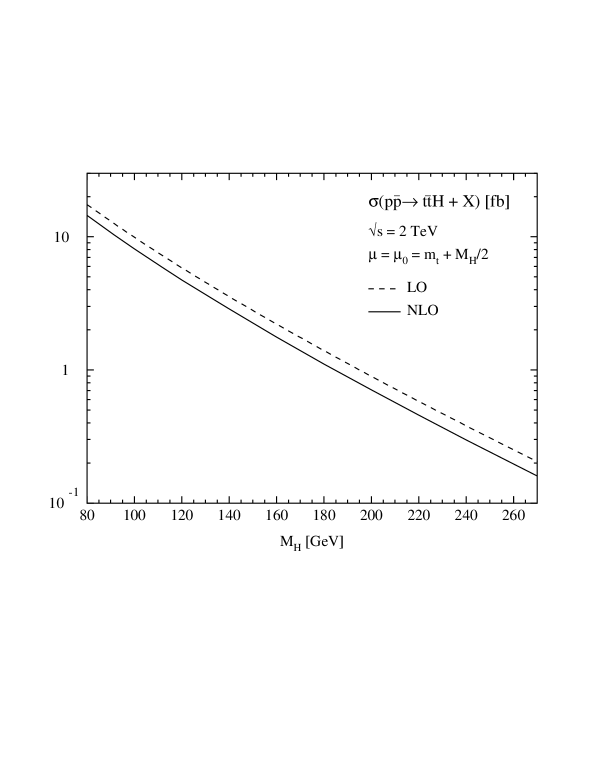
Figure 7: Total cross section for $\,p\bar{p}\to t\bar{t}H+X$ at the Tevatron in LO and NLO approximation, with the renormalization and factorization scales set to $\mu_{0}=(2m_{t}+M_{H})/2$.

Figure 8: Variation of the LO and NLO cross sections with the renormalization and factorization scales for $\,p\bar{p}\to t\bar{t}H$ at the Tevatron.

Figure 9: Total cross section for $\,pp\to t\bar{t}H+X$ at the LHC in LO and NLO approximation, with the renormalization and factorization scales set to $\mu_{0}=(2m_{t}+M_{H})/2$.

Figure 10: Variation of the LO and NLO cross sections with the renormalization and factorization scales for $\,pp\to t\bar{t}H$ at the LHC.

		MRST(LO/NLO)				CTEQ6
	$M_{H}$ [GeV]	$\sigma_{\mathrm{LO}}$ [fb]	$\sigma_{\mathrm{NLO}}$ [fb]	$K$	$q\bar{q}:gg$ (LO)	$\sigma_{\mathrm{NLO}}$ [fb]
	120	5.846(2)	4.857(8)	0.83	0.99 : 0.01	4.871(8)
	140	3.551(1)	2.925(4)	0.82	0.99 : 0.01	2.931(5)
Tevatron	160	2.205(1)	1.806(2)	0.82	0.99 : 0.01	1.808(3)
	180	1.393(1)	1.132(1)	0.81	0.996 : 0.004	1.133(2)
	120	577.3(4)	701.5(18)	1.22	0.30 : 0.70	665.0(19)
	140	373.4(3)	452.3(12)	1.21	0.33 : 0.67	431.8(13)
LHC	160	251.6(2)	305.6(8)	1.21	0.35 : 0.65	290.6(8)
	180	176.0(1)	214.0(6)	1.22	0.36 : 0.64	203.4(5)

Table 1: Total cross sections and $K$ factors for $\,p\bar{p}\to t\bar{t}H$ at the Tevatron and for $\,pp\to t\bar{t}H$ at the LHC. The renormalization and factorization scales have been set to $\mu=\mu_{0}=(2m_{t}+M_{H})/2$. The MRST [47] parton densities have been adopted as default, whereas in the rightmost column a comparison is performed with the CTEQ6 [49] parton densities. The relative weight of $q\bar{q}$ and $gg$ initial states at LO is given in the second-to-last column.

As argued in Section 3.1, the impact of the Coulomb singularity and the threshold logarithms from soft-gluon radiation is suppressed because of the $\beta^{4}$ behaviour of the massive three-particle phase space near threshold. Nevertheless the threshold region gives us insight into the different colour factors that determine the NLO corrections at the Tevatron and the LHC. Just like the partonic high-energy region, where the fragmentation picture applies and the high-energy plateaus dominate the NLO corrections, also the low-energy threshold region hints at $K$ factors at the LHC that are substantially larger than the ones at the Tevatron (see Section 2.4).

We have also studied the uncertainty in the cross-section prediction due to the error in the parametrization of the parton densities. To this end we have compared the NLO cross section evaluated using the default MRST [47] parametrization with the cross section evaluated using the CTEQ6 [49] parametrization. The results are collected in the rightmost column of Table 1. Both MRST and CTEQ include a systematic treatment of parton-distribution-function uncertainties and provide the means for a quantitative estimate of the corresponding uncertainties in the cross sections. Using the parton-distribution-error packages [47, 49], we find that the uncertainty due to the parametrization of the parton densities in NLO is less than $\approx 5\%$ at the Tevatron, where the quark–antiquark initial states dominate, and less than $\approx 10\%$ at the LHC, where gluon–gluon initial states are more prominent.

3.2.2 Differential distributions

In Figs. 11–15 the normalized transverse-momentum and rapidity distributions of the Higgs boson and the top quarks [$t$ and $\bar{t}$ not discriminated] are shown for $\,p\bar{p}\to t\bar{t}H$ at the Tevatron in LO and NLO approximation. For the transverse-momentum distributions we choose the transverse mass as the default renormalization and factorization scale, i.e. $\mu^{2}=p_{T,H}^{2}+M_{H}^{2}$ and $\mu^{2}=p_{T,t/\bar{t}}^{2}+m_{t}^{2}$ for Higgs-boson and top/antitop distributions, respectively, which provides a more natural choice for large transverse momenta.

The scale dependence of the distributions in rapidity and transverse momentum of the Higgs boson and top quarks is greatly reduced at NLO. The improvement is exemplified in Fig. 11 which compares the transverse-momentum distribution of the Higgs boson, once calculated with the renormalization and factorization scales set to the transverse mass, and once with both scales fixed to $\mu_{0}$. We observe differences of up to $30\%$ at LO, while the shape of the $p_{T,H}$ distribution at NLO is practically identical for the two choices of scales.

The ratio of the (normalized) NLO and LO transverse-momentum distributions of the Higgs boson, displayed in the insert in Fig. 13, reveals that the simple rescaling of the LO $p_{T,H}$ distribution by a constant $K$ factor reproduces the NLO distribution only within $\pm 10\%$ in the relevant transverse-momentum range, if the transverse mass is chosen as the scale. The increase of the ratio $\mbox{d}\sigma_{\mathrm{NLO}}/\mbox{d}\sigma_{\mathrm{LO}}$ with increasing $p_{T,H}$ can be understood in terms of the scale dependences of $\mbox{d}\sigma_{\mathrm{NLO}}$ and $\mbox{d}\sigma_{\mathrm{LO}}$: with $\mu^{2}=p_{T,H}^{2}+M_{H}^{2}$ rising with increasing $p_{T,H}$, $\mbox{d}\sigma_{\mathrm{LO}}$ decreases with increasing $\mu$ faster than $\mbox{d}\sigma_{\mathrm{NLO}}$ (see Fig. 8). We note that choosing a fixed scale for the LO $p_{T,H}$ distribution provides a better description of the NLO shape.

For the transverse-momentum distribution of the top quarks, the increase of the ratio $\mbox{d}\sigma_{\mathrm{NLO}}/\mbox{d}\sigma_{\mathrm{LO}}$ with increasing $p_{T,H}$ due to the scale dependence is balanced by gluon radiation off top quarks at NLO, which reduces the energies and momenta of the top particles and thereby depletes the region of large transverse momenta. As a net result, the shape of the transverse-momentum distribution of the top quarks is barely affected by the NLO corrections in the relevant range $p_{T,t/\bar{t}}\,\mathrel{\raisebox{-3.00003pt}{$\stackrel{{\scriptstyle\displaystyle<}}{{\sim}}$}}\,300\,\mathrm{GeV}$, if the transverse top-quark mass is adopted for the renormalization and factorization scales (see Fig. 15).

The reduction in energies and momenta of the massive final-state particles due to gluon radiation at NLO is also expected to enhance the central rapidity region. However, as evident from Figs. 13 and 15, the effect on the (normalized) rapidity distributions of the massive final-state particles is small and becomes noticeable at the edges of phase space only.

Cum grano salis, the transverse-momentum and rapidity distributions of the Higgs boson and the top quarks for $\,pp\to t\bar{t}H$ at the LHC, Figs. 17–19, show the same qualitative behaviour as observed for the Tevatron. Adopting the Higgs transverse mass as the scale, the difference between the NLO and LO Higgs-boson transverse-momentum distributions at the LHC is naturally more pronounced, with deviations of up to $30\%$ at large $p_{T,H}$. As for the Tevatron, choosing a fixed scale for the LO $p_{T,H}$ distribution provides a better description of the NLO shape.

4 Summary

In this report we have presented the theoretical analysis of the Standard-Model processes $p\bar{p}/pp\to t\bar{t}H+X$ in next-to-leading order QCD at the Tevatron and the LHC. We have focussed on two aspects.

(i) The technical basis for the prediction of the cross sections has been elaborated in detail. Particular emphasis has been put on evaluating pentagon diagrams, which involves the isolation of the singularities, the reduction to lower $n$-point functions, and the stable integration over the phase space. As a second important technical element we have applied the dipole subtraction formalism to treat massive final-state particles. In fact, the processes reported on here, represent the first complex examples that have been treated in this formalism in the case of massive quarks.

(ii) In expanding on results presented in an earlier letter, Ref. [10], we have analyzed not only the total cross sections for Higgs bremsstrahlung off top quarks at the Tevatron and the LHC, but also final-state rapidity and transverse-momentum distributions for the Higgs boson and the top quarks. Moreover, we have studied the uncertainty in the next-to-leading order cross section prediction due to different parametrizations of the parton densities.

When including higher-order QCD corrections, the $K$ factor at the Tevatron has a value slightly below unity. It varies between $\sim 0.8$ and $\sim 1.0$ for renormalization and factorization scales between $\mu=\mu_{0}$ and $2\mu_{0}$, almost independent of the Higgs-boson mass in the intermediate range. Here $2\mu_{0}=2m_{t}+M_{H}$ denotes the threshold CM energy of the partonic subprocesses. Similarly, the $K$ factor varies between $\sim 1.2$ and $\sim 1.4$ for the same scales at the LHC. Most importantly, the NLO predictions for the total cross sections and for the distributions in rapidity and transverse momentum of the Higgs boson and top quarks are stable when the renormalization and factorization scales are varied, in contrast to the Born approximation. The improved cross sections can therefore serve as a solid base for experimental analyses at the Tevatron and the LHC.

Appendix

Appendix A The IR-divergent scalar 3- and 4-point integrals

In this first appendix all relevant IR-divergent scalar 3- and 4-point integrals are listed. They have been derived in two independent ways, once with the help of Feynman parametrization, once by means of cutting techniques and dispersion integrals. In the following the momenta $p_{i}$ are defined as in Section 2.1, i.e. they are on shell: $p_{1}^{2}=p_{2}^{2}=0$, $p_{3}^{2}=p_{4}^{2}=m_{t}^{2}$, $p_{5}^{2}=M_{H}^{2}$. Throughout this appendix we make extensive use of the quantities

$$\beta_{r}=\sqrt{1-\frac{4m_{t}^{2}}{\bar{r}}},\qquad x_{r}=\frac{\beta_{r}-1}{\beta_{r}+1},$$ (A.1)

where $r$ represents a generic invariant. Moreover, we adopt the convention that invariants with a bar receive an infinitesimally small, positive imaginary part: $\bar{r}=r+{\mathrm{i}}0$.

There are four different IR-divergent 3-point functions that become relevant. In $D\neq 4$ dimensions they read

$$C^{(D)}_{0}(p_{1},-p_{2},0,0,0) = \frac{1}{\hat{s}}\Biggl{[}\Delta^{\mathrm{IR}}_{2}(\mu)-\Delta^{\mathrm{IR}}_{1}(\mu)\ln\biggl{(}\frac{{}-\bar{\hat{s}}\,}{m_{t}^{2}}\biggr{)}+\frac{1}{2}\ln^{2}\biggl{(}\frac{{}-\bar{\hat{s}}\,}{m_{t}^{2}}\biggr{)}-\frac{\pi^{2}}{6}\Biggr{]},$$

$$C^{(D)}_{0}(p_{1},p_{1}-p_{3},0,0,m_{t}) = \frac{1}{t_{13}-m_{t}^{2}}\Biggl{[}\frac{1}{2}\Delta^{\mathrm{IR}}_{2}(\mu)-\Delta^{\mathrm{IR}}_{1}(\mu)\ln\biggl{(}1-\frac{\bar{t}_{13}}{m_{t}^{2}}\biggr{)}+\mathop{\mathrm{Li}_{2}}\nolimits\biggl{(}\frac{\bar{t}_{13}}{m_{t}^{2}}\biggr{)}$$

$$\qquad{}+\ln^{2}\biggl{(}1-\frac{\bar{t}_{13}}{m_{t}^{2}}\biggr{)}\Biggr{]},$$

$$C^{(D)}_{0}(p_{1},p_{4}+p_{5},0,0,m_{t}) = \frac{1}{s_{45}-t_{23}}\Biggl{[}\Delta^{\mathrm{IR}}_{1}(\mu)\ln\biggl{(}\frac{\bar{t}_{23}-m_{t}^{2}}{\bar{s}_{45}-m_{t}^{2}}\biggr{)}+\mathop{\mathrm{Li}_{2}}\nolimits\biggl{(}\frac{\bar{s}_{45}}{m_{t}^{2}}\biggr{)}-\mathop{\mathrm{Li}_{2}}\nolimits\biggl{(}\frac{\bar{t}_{23}}{m_{t}^{2}}\biggr{)}$$

$$\qquad{}+\ln^{2}\biggl{(}1-\frac{\bar{s}_{45}}{m_{t}^{2}}\biggr{)}-\ln^{2}\biggl{(}1-\frac{\bar{t}_{23}}{m_{t}^{2}}\biggr{)}\Biggr{]},$$

$$C^{(D)}_{0}(p_{3},-p_{4},0,m_{t},m_{t}) = \frac{1}{s_{34}\beta_{s_{34}}}\Biggl{[}\Delta^{\mathrm{IR}}_{1}(\mu)\ln(x_{s_{34}})-2\mathop{\mathrm{Li}_{2}}\nolimits({}-x_{s_{34}})$$ (A.2)

$$\qquad{}-2\ln(x_{s_{34}})\,\ln(1+x_{s_{34}})+\frac{1}{2}\,\ln^{2}(x_{s_{34}})-\frac{\pi^{2}}{6}\Biggr{]}.$$

We also present these 3-point functions with mass regularization, where all internal massless particles are endowed with an infinitesimally small mass $\lambda$:

$$C^{(\mathrm{mass},D=4)}_{0}(p_{1},-p_{2},\lambda,\lambda,\lambda) = \frac{1}{2\hat{s}}\ln^{2}\biggl{(}\frac{{}-\bar{\hat{s}}\,}{\lambda^{2}}\biggr{)},$$

$$C^{(\mathrm{mass},D=4)}_{0}(p_{1},p_{1}-p_{3},\lambda,\lambda,m_{t}) = \frac{1}{t_{13}-m_{t}^{2}}\Biggl{[}\ln^{2}\biggl{(}\frac{m_{t}^{2}-\bar{t}_{13}}{\lambda m_{t}}\biggr{)}+\mathop{\mathrm{Li}_{2}}\nolimits\biggl{(}\frac{\bar{t}_{13}}{m_{t}^{2}}\biggr{)}+\frac{\pi^{2}}{12}\Biggr{]},$$

$$C^{(\mathrm{mass},D=4)}_{0}(p_{1},p_{4}+p_{5},\lambda,\lambda,m_{t}) = \frac{1}{s_{45}-t_{23}}\Biggl{[}\ln^{2}\biggl{(}\frac{m_{t}^{2}-\bar{s}_{45}}{\lambda m_{t}}\biggr{)}-\ln^{2}\biggl{(}\frac{m_{t}^{2}-\bar{t}_{23}}{\lambda m_{t}}\biggr{)}$$

$$\qquad{}+\mathop{\mathrm{Li}_{2}}\nolimits\biggl{(}\frac{\bar{s}_{45}}{m_{t}^{2}}\biggr{)}-\mathop{\mathrm{Li}_{2}}\nolimits\biggl{(}\frac{\bar{t}_{23}}{m_{t}^{2}}\biggr{)}\Biggr{]},$$

$$C^{(\mathrm{mass},D=4)}_{0}(p_{3},-p_{4},\lambda,m_{t},m_{t}) = \frac{1}{s_{34}\beta_{s_{34}}}\Biggl{[}\ln\biggl{(}\frac{\lambda^{2}}{m_{t}^{2}}\biggr{)}\ln(x_{s_{34}})-2\mathop{\mathrm{Li}_{2}}\nolimits({}-x_{s_{34}})$$

$$\qquad{}-2\ln(x_{s_{34}})\,\ln(1+x_{s_{34}})+\frac{1}{2}\,\ln^{2}(x_{s_{34}})-\frac{\pi^{2}}{6}\Biggr{]}.$$

Taking into account that the decomposition of the 5-point integrals leads to additional 4-point integrals, six different IR-divergent 4-point integrals are needed:

$$D^{(D)}_{0}(p_{1},p_{1}-p_{3},-p_{2},0,0,m_{t},0)=\frac{1}{\hat{s}(t_{13}-m_{t}^{2})}$$

$${}\times\Biggl{[}\frac{3}{2}\Delta^{\mathrm{IR}}_{2}(\mu)-\Delta^{\mathrm{IR}}_{1}(\mu)\biggl{\{}2\ln\biggl{(}1-\frac{\bar{t}_{13}}{m_{t}^{2}}\biggr{)}+\ln\biggl{(}\frac{{}-\bar{\hat{s}}\,}{m_{t}^{2}}\biggr{)}-\ln\biggl{(}1-\frac{\bar{s}_{45}}{m_{t}^{2}}\biggr{)}\biggr{\}}$$

$$\qquad{}-2\mathop{\mathrm{Li}_{2}}\nolimits\biggl{(}\frac{\bar{t}_{13}-\bar{s}_{45}}{\bar{t}_{13}-m_{t}^{2}}\biggr{)}+2\ln\biggl{(}\frac{{}-\bar{\hat{s}}\,}{m_{t}^{2}}\biggr{)}\ln\biggl{(}1-\frac{\bar{t}_{13}}{m_{t}^{2}}\biggr{)}-\ln^{2}\biggl{(}1-\frac{\bar{s}_{45}}{m_{t}^{2}}\biggr{)}-\frac{2\pi^{2}}{3}\Biggr{]},\hskip 20.00003pt$$

$$D^{(D)}_{0}(p_{1},p_{1}-p_{3},p_{4}+p_{5},0,0,m_{t},m_{t})=\frac{1}{(t_{13}-m_{t}^{2})(t_{23}-m_{t}^{2})}$$

$${}\times\Biggl{[}\frac{1}{2}\Delta^{\mathrm{IR}}_{2}(\mu)-\Delta^{\mathrm{IR}}_{1}(\mu)\biggl{\{}\ln\biggl{(}1-\frac{\bar{t}_{13}}{m_{t}^{2}}\biggr{)}+\ln\biggl{(}1-\frac{\bar{t}_{23}}{m_{t}^{2}}\biggr{)}-\ln\biggl{(}1-\frac{\bar{s}_{45}}{m_{t}^{2}}\biggr{)}\biggr{\}}$$

$$\qquad{}-2\mathop{\mathrm{Li}_{2}}\nolimits\biggl{(}\frac{\bar{t}_{23}-\bar{s}_{45}}{\bar{t}_{23}-m_{t}^{2}}\biggr{)}-2\mathop{\mathrm{Li}_{2}}\nolimits\biggl{(}\frac{\bar{t}_{13}-\bar{s}_{45}}{\bar{t}_{13}-m_{t}^{2}}\biggr{)}+2\ln\biggl{(}1-\frac{\bar{t}_{13}}{m_{t}^{2}}\biggr{)}\ln\biggl{(}1-\frac{\bar{t}_{23}}{m_{t}^{2}}\biggr{)}$$

$$\qquad{}-\ln^{2}\biggl{(}1-\frac{\bar{s}_{45}}{m_{t}^{2}}\biggr{)}-\frac{\pi^{2}}{6}\Biggr{]},$$

$$D^{(D)}_{0}(p_{1},p_{1}-p_{3},p_{4},0,0,m_{t},m_{t})=\frac{1}{(t_{13}-m_{t}^{2})(t_{14}-m_{t}^{2})}$$

$${}\times\Biggl{[}\Delta^{\mathrm{IR}}_{2}(\mu)-\Delta^{\mathrm{IR}}_{1}(\mu)\biggl{\{}\ln\biggl{(}1-\frac{\bar{t}_{14}}{m_{t}^{2}}\biggr{)}+\ln\biggl{(}1-\frac{\bar{t}_{13}}{m_{t}^{2}}\biggr{)}\biggr{\}}-\ln^{2}(x_{t_{25}})$$

$$\qquad{}+2\ln\biggl{(}1-\frac{\bar{t}_{13}}{m_{t}^{2}}\biggr{)}\ln\biggl{(}1-\frac{\bar{t}_{14}}{m_{t}^{2}}\biggr{)}-\frac{2\pi^{2}}{3}\Biggr{]},$$

$$D^{(D)}_{0}(p_{1},p_{1}-p_{3},p_{4}-p_{2},0,0,m_{t},m_{t})=\frac{1}{(t_{13}-m_{t}^{2})(s_{35}-m_{t}^{2})}$$

$${}\times\Biggl{[}\frac{1}{2}\Delta^{\mathrm{IR}}_{2}(\mu)-\Delta^{\mathrm{IR}}_{1}(\mu)\biggl{\{}\ln\biggl{(}1-\frac{\bar{t}_{13}}{m_{t}^{2}}\biggr{)}+\ln\biggl{(}1-\frac{\bar{s}_{35}}{m_{t}^{2}}\biggr{)}-\ln\biggl{(}1-\frac{\bar{t}_{24}}{m_{t}^{2}}\biggr{)}\biggr{\}}$$

$$\qquad{}-\sum_{\rho=\pm 1}\mathop{{\cal L}i_{2}}\nolimits\biggl{(}\frac{\bar{t}_{24}-m_{t}^{2}}{\bar{t}_{13}-m_{t}^{2}},x_{M_{H}^{2}}^{\,\rho}\biggr{)}-2\,\mathop{\mathrm{Li}_{2}}\nolimits\biggl{(}\frac{\bar{s}_{35}-\bar{t}_{24}}{\bar{s}_{35}-m_{t}^{2}}\biggr{)}+2\ln\biggl{(}1-\frac{\bar{t}_{13}}{m_{t}^{2}}\biggr{)}\ln\biggl{(}1-\frac{\bar{s}_{35}}{m_{t}^{2}}\biggr{)}$$

$$\qquad{}-\ln^{2}\biggl{(}1-\frac{\bar{t}_{24}}{m_{t}^{2}}\biggr{)}-\ln^{2}(x_{M_{H}^{2}})-\frac{\pi^{2}}{6}\Biggr{]},$$

$$D^{(D)}_{0}(p_{3},p_{3}-p_{1},-p_{4},0,m_{t},m_{t},m_{t})=\frac{1}{(t_{13}-m_{t}^{2})s_{34}\beta_{s_{34}}}$$

$${}\times\Biggl{[}\Delta^{\mathrm{IR}}_{1}(\mu)\ln(x_{s_{34}})-2\sum_{\rho=\pm 1}\mathop{{\cal L}i_{2}}\nolimits(x_{s_{34}},x_{t_{25}}^{\,\rho})-\mathop{\mathrm{Li}_{2}}\nolimits(x_{s_{34}}^{2})-2\ln(x_{s_{34}})\ln(1-x_{s_{34}}^{2})$$

$$\qquad{}-2\ln(x_{s_{34}})\ln\biggl{(}1-\frac{\bar{t}_{13}}{m_{t}^{2}}\biggr{)}-\ln^{2}(x_{t_{25}})+\frac{\pi^{2}}{6}\Biggr{]},$$

$$D^{(D)}_{0}(p_{3},p_{3}+p_{5},-p_{4},0,m_{t},m_{t},m_{t})=\frac{1}{(s_{35}-m_{t}^{2})s_{34}\beta_{s_{34}}}$$ (A.4)

$${}\times\Biggl{[}\Delta^{\mathrm{IR}}_{1}(\mu)\ln(x_{s_{34}})-\sum_{\rho,\,\sigma=\pm 1}\mathop{{\cal L}i_{2}}\nolimits(x_{s_{34}},x_{\hat{s}}^{\,\rho},x_{M_{H}^{2}}^{\sigma})-\mathop{\mathrm{Li}_{2}}\nolimits(x_{s_{34}}^{2})-2\ln(x_{s_{34}})\ln(1-x_{s_{34}}^{2})$$

$$\qquad{}-2\ln(x_{s_{34}})\ln\biggl{(}1-\frac{\bar{s}_{35}}{m_{t}^{2}}\biggr{)}-\ln^{2}(x_{\hat{s}})-\ln^{2}(x_{M_{H}^{2}})+\frac{\pi^{2}}{6}\Biggr{]}.$$

The following specific combinations of logarithms and dilogarithms were used,

$$\mathop{{\cal L}i_{2}}\nolimits(x,y) = \mathop{\mathrm{Li}_{2}}\nolimits(1-xy)+\ln(1-xy)\,\Bigl{[}\ln(xy)-\ln(x)-\ln(y)\Bigr{]},$$

$$\mathop{{\cal L}i_{2}}\nolimits(x,y,z) = \mathop{\mathrm{Li}_{2}}\nolimits(1-xyz)+\ln(1-xyz)\,\Bigl{[}\ln(xyz)-\ln(x)-\ln(y)-\ln(z)\Bigr{]}.$$ (A.5)

The expressions given for the $C_{0}$ and $D_{0}$ functions are valid for arbitrary real values of the variables $\hat{s},s_{ij}$, $t_{ij}$, and $M_{H}^{2}$, independent of their kinematical range.

The method described in Section 2.2.3 (ii) can also be used to calculate the singularities of the 4-point functions $D_{0}$ in terms of 3-point functions $C_{0}$. The corresponding relations between $D_{0,\mathrm{sing}}$ and the 3-point subintegrals are

$$D_{0}(p_{1},p_{1}-p_{3},-p_{2},0,0,m_{t},0)_{\mathrm{sing}}=\frac{1}{t_{13}-m_{t}^{2}}\,C_{0}(p_{1},-p_{2},0,0,0)$$

$${}+\frac{t_{13}-s_{45}}{\hat{s}(t_{13}-m_{t}^{2})}\,C_{0}(p_{1}-p_{3},-p_{2},0,m_{t},0)+\frac{1}{\hat{s}}\,C_{0}(p_{1},p_{1}-p_{3},0,0,m_{t}),\hskip 40.00006pt$$

$$D_{0}(p_{1},p_{1}-p_{3},p_{4}+p_{5},0,0,m_{t},m_{t})_{\mathrm{sing}}=\frac{1}{t_{23}-m_{t}^{2}}\,C_{0}(p_{1},p_{1}-p_{3},0,0,m_{t})$$

$${}+\frac{t_{23}-s_{45}}{(t_{13}-m_{t}^{2})(t_{23}-m_{t}^{2})}\,C_{0}(p_{1},p_{4}+p_{5},0,0,m_{t}),$$

$$D_{0}(p_{1},p_{1}-p_{3},p_{4},0,0,m_{t},m_{t})_{\mathrm{sing}}=\frac{1}{t_{14}-m_{t}^{2}}\,C_{0}(p_{1},p_{1}-p_{3},0,0,m_{t})$$

$${}+\frac{1}{t_{13}-m_{t}^{2}}\,C_{0}(p_{1},p_{4},0,0,m_{t}),$$

$$D_{0}(p_{1},p_{1}-p_{3},p_{4}-p_{2},0,0,m_{t},m_{t})_{\mathrm{sing}}=\frac{1}{s_{35}-m_{t}^{2}}\,C_{0}(p_{1},p_{1}-p_{3},0,0,m_{t})$$

$${}+\frac{s_{35}-t_{24}}{(t_{13}-m_{t}^{2})(s_{35}-m_{t}^{2})}\,C_{0}(p_{1},p_{4}-p_{2},0,0,m_{t}),$$

$$D_{0}(p_{3},p_{3}-p_{1},-p_{4},0,m_{t},m_{t},m_{t})_{\mathrm{sing}}=\frac{1}{t_{13}-m_{t}^{2}}\,C_{0}(p_{3},-p_{4},0,m_{t},m_{t}),$$

$$D_{0}(p_{3},p_{3}+p_{5},-p_{4},0,m_{t},m_{t},m_{t})_{\mathrm{sing}}=\frac{1}{s_{35}-m_{t}^{2}}\,C_{0}(p_{3},-p_{4},0,m_{t},m_{t}).$$ (A.6)

Obviously the explicit results for $D^{(D)}_{0}$ and $C^{(D)}_{0}$ given above are compatible with these relations. Moreover, the functions $D_{0,\mathrm{sing}}$ can be used to translate the $D$-dimensional $D_{0}$ functions of Eq. (A.4) into their mass-regularized counterparts $D_{0}^{(\mathrm{mass},D=4)}$,

$$D_{0}^{(\mathrm{mass},D=4)}=D^{(\mathrm{mass},D=4)}_{0,\mathrm{sing}}+\left[D_{0}^{(D)}-D^{(D)}_{0,\mathrm{sing}}\right]+\dots,$$ (A.7)

where the $C_{0}$ functions occurring in $D^{(D)}_{0,\mathrm{sing}}$ and $D^{(\mathrm{mass},D=4)}_{0,\mathrm{sing}}$ are given in Eqs. (A.2) and (LABEL:eq:C0mass), respectively, or result from those by mere substitutions. The dots represent infinitesimally small terms proportional to the regulators $(\,D\!-\!4\,)$ or $\lambda$.

A simple example:

$$D_{0}^{(\mathrm{mass},D=4)}(p_{3},p_{3}-p_{1},-p_{4},\lambda,m_{t},m_{t},m_{t})=\frac{1}{t_{13}-m_{t}^{2}}\,C_{0}^{(\mathrm{mass},D=4)}(p_{3},-p_{4},\lambda,m_{t},m_{t})$$ (A.8)

$$\quad{}+D_{0}^{(D)}(p_{3},p_{3}-p_{1},-p_{4},0,m_{t},m_{t},m_{t})-\frac{1}{t_{13}-m_{t}^{2}}\,C_{0}^{(D)}(p_{3},-p_{4},0,m_{t},m_{t})+\dots$$

$$= \frac{1}{(t_{13}-m_{t}^{2})s_{34}\beta_{s_{34}}}\Biggl{[}\ln\biggl{(}\frac{\lambda^{2}}{m_{t}^{2}}\biggr{)}\ln(x_{s_{34}})-2\sum_{\rho=\pm 1}\mathop{{\cal L}i_{2}}\nolimits(x_{s_{34}},x_{t_{25}}^{\,\rho})-\mathop{\mathrm{Li}_{2}}\nolimits(x_{s_{34}}^{2})$$

$$\qquad{}-2\ln(x_{s_{34}})\ln(1-x_{s_{34}}^{2})-2\ln(x_{s_{34}})\ln\biggl{(}1-\frac{\bar{t}_{13}}{m_{t}^{2}}\biggr{)}-\ln^{2}(x_{t_{25}})+\frac{\pi^{2}}{6}\Biggr{]},$$

which agrees with the result in the literature [29]. So, by subtracting and adding well-defined singular integrals we are able to switch between arbitrary regularization schemes. For instance, to switch to an off-shell regularization scheme, with some of the external particles put slightly off-shell, it is sufficient to know the relevant 3-point integrals in that scheme.

Appendix B Colour operators and correlations

In order to make the results in this report as compact as possible, colour indices have been suppressed in the expressions by making use of colour operators. The definitions of these colour operators are given in this appendix (see also Refs. [23, 24, 36]).

Consider the matrix element for a process involving $n$ coloured external particles, ${\cal{M}}^{a_{1}\,\ldots\,a_{n}}$, where $\,a_{1},\dots,a_{n}\,$ are the colour indices of the coloured particles. These colour indices range from 1 to 8 for gluons [adjoint representation] and from 1 to 3 for (anti)quarks [fundamental representation]. Emission of a gluon with colour index $c$ from the external particle $j$ is represented by a specific colour operator (charge) ${\bf T}_{j}$ acting on the matrix element:

$$({\cal{M}}\otimes{\bf T}_{j})^{c;\,a_{1}\,\ldots\,a_{n}}=\sum_{b_{1},\,\ldots\,,\,b_{n}}\delta_{a_{1}b_{1}}\cdots\,(T_{j}^{\,c})_{a_{j}b_{j}}\cdots\,\delta_{a_{n}b_{n}}\,{\cal{M}}^{b_{1}\,\ldots\,b_{n}}\ =\ \sum_{b_{j}}\,(T_{j}^{\,c})_{a_{j}b_{j}}\,{\cal{M}}^{a_{1}\,\ldots\,b_{j}\,\ldots\,a_{n}},$$ (B.1)

with $(T_{j}^{\,c})_{ab}={}-if_{cab}\,$ for incoming/outgoing gluons, $(T_{j}^{\,c})_{ab}=\lambda^{c}_{ab}/2\,$ for outgoing quarks or incoming antiquarks, and $(T_{j}^{\,c})_{ab}={}-\lambda^{c}_{ba}/2\,$ for outgoing antiquarks or incoming quarks. Owing to $SU(3)$ gauge invariance, the complete matrix element ${\cal{M}}$ is a colour singlet. This leads to the colour-conservation identity

$$\sum_{j=1}^{n}({\cal{M}}\otimes{\bf T}_{j})^{c;\,a_{1}\,\ldots\,a_{n}}=0.$$ (B.2)

In the NLO calculations the colour operators enter as products $({\bf T}_{j}\cdot{\bf T}_{k})=({\bf T}_{k}\cdot{\bf T}_{j})$, defined according to

$$[{\cal{M}}\otimes({\bf T}_{j}\cdot{\bf T}_{k})]^{a_{1}\,\ldots\,a_{n}}=\sum_{b_{j},\,b_{k}}\,\sum_{c}\,(T_{j}^{\,c})_{a_{j}b_{j}}\,(T_{k}^{\,c})_{a_{k}b_{k}}\,{\cal{M}}^{a_{1}\,\ldots\,b_{j}\,\ldots\,b_{k}\,\ldots\,a_{n}}\qquad\mbox{if \ $j\neq k$},$$

$$[{\cal{M}}\otimes{\bf T}_{j}^{2}\,]^{a_{1}\,\ldots\,a_{n}}=\sum_{b_{j},\,c_{j}}\,\sum_{c}\,(T_{j}^{\,c})_{a_{j}c_{j}}\,(T_{j}^{\,c})_{c_{j}b_{j}}\,{\cal{M}}^{a_{1}\,\ldots\,b_{j}\,\ldots\,a_{n}}\ =\ C_{j}\,{\cal{M}}^{a_{1}\,\ldots\,a_{n}}.$$ (B.3)

Here $C_{j}$ is the Casimir operator in the representation of particle $j$, i.e. ${\bf T}_{j}^{2}=C_{\mathrm{A}}=3\,$ for gluons [adjoint representation] and ${\bf T}_{j}^{2}=C_{\mathrm{F}}=4/3\,$ for (anti)quarks [fundamental representation]. At the cross-section level this gives rise to colour correlations of the form

$$\sum_{\mathrm{colours}}|{\cal{M}}|^{2}\otimes({\bf T}_{j}\cdot{\bf T}_{k})=\sum_{a_{1},\,\ldots\,,\,a_{n}}\Bigl{[}{\cal{M}}^{a_{1}\,\ldots\,a_{n}}\Bigr{]}^{*}\,\sum_{b_{j},\,b_{k}}\,\sum_{c}\,(T_{j}^{\,c})_{a_{j}b_{j}}\,(T_{k}^{\,c})_{a_{k}b_{k}}\,{\cal{M}}^{a_{1}\,\ldots\,b_{j}\,\ldots\,b_{k}\,\ldots\,a_{n}}$$ (B.4)

for $j\neq k$. Needless to say that the left-hand side of Eq. (B.4) looks much more appealing from the point of view of compact expressions.

Finally, we give the explicit results for the colour correlations in terms of the colour operators ${\cal C}^{q\bar{q}}$ and ${\cal C}^{gg}_{m}$ defined in Eqs. (2.6) and (2.14), respectively. Since these ${\cal C}$ operators represent a basis for the relevant colour structures of the $q\bar{q}$ and $gg$ channels, the correlations ${\cal C}\otimes({\bf T}_{j}\cdot{\bf T}_{k})$ can again be expanded in terms of ${\cal C}$’s:

$${\cal C}^{q\bar{q}}\otimes({\bf T}_{j}\cdot{\bf T}_{k})\ =\ \xi^{q\bar{q}}_{jk}\,{\cal C}^{q\bar{q}}+\dots,\qquad{\cal C}^{gg}_{m}\otimes({\bf T}_{j}\cdot{\bf T}_{k})\ =\ \sum_{n=1}^{3}\xi^{gg,mn}_{jk}\,{\cal C}^{gg}_{n},$$ (B.5)

where the dots stand for (irrelevant) operators orthogonal to ${\cal C}^{q\bar{q}}$. The coefficients $\xi$ follow from simple colour algebra. For the $q\bar{q}$ channel they read

$$\xi^{q\bar{q}}_{12}=\xi^{q\bar{q}}_{34}=\frac{1}{6},\quad\xi^{q\bar{q}}_{13}=\xi^{q\bar{q}}_{24}=-\frac{7}{6},\quad\xi^{q\bar{q}}_{14}=\xi^{q\bar{q}}_{23}=-\frac{1}{3}.$$ (B.6)

For $gg$ fusion it is convenient to give them in matrix form,

$$\left(\xi^{gg,mn}_{12}\right) \ =\ \mathrm{diag}\left(-3,-\frac{3}{2},-\frac{3}{2}\right),\qquad\left(\xi^{gg,mn}_{34}\right)\ =\ \mathrm{diag}\left(-\frac{4}{3},\frac{1}{6},\frac{1}{6}\right),$$

$$\left(\xi^{gg,mn}_{13}\right) \ =\ \left(\xi^{gg,mn}_{24}\right)\ =\ \pmatrix{\vphantom{{X^{X}}^{X}}0&-\frac{1}{2}&0\cr\vphantom{{X^{X}}^{X}}-1&-\frac{3}{4}&-\frac{3}{4}\cr\vphantom{{X^{X}}^{X}}0&-\frac{5}{12}&-\frac{3}{4}},$$

$$\left(\xi^{gg,mn}_{14}\right) \ =\ \left(\xi^{gg,mn}_{23}\right)\ =\ \pmatrix{\vphantom{{X^{X}}^{X}}0&\frac{1}{2}&0\cr\vphantom{{X^{X}}^{X}}1&-\frac{3}{4}&\frac{3}{4}\cr\vphantom{{X^{X}}^{X}}0&\frac{5}{12}&-\frac{3}{4}}.$$ (B.7)

These $\xi$ coefficients have also been used in Section 2.2.5 in rewriting Eqs. (2.45) and (2.46) in terms of Eq. (2.48).

Appendix C The Altarelli–Parisi splitting functions at NLO

The so-called Altarelli–Parisi splitting functions $P^{ab}(x)$ [50] are a measure of the probability of finding the parton $b$ with fraction $x$ of longitudinal momentum inside the parent parton $a$. At NLO these splitting functions can be written in terms of a regularized splitting function and an IR-sensitive part according to

$$P^{ab}(x)=P_{\mathrm{reg}}^{ab}(x)+\delta^{ab}\biggl{[}2\,{\bf T}_{a}^{2}\,\left(\frac{1}{1-x}\right)_{+}+\gamma_{a}\,\delta(1-x)\biggr{]}.$$ (C.1)

The anomalous dimensions $\gamma_{a}$ are given by

$$\gamma_{q}=\gamma_{\bar{q}}=\frac{3}{2}\,C_{\mathrm{F}}=2\qquad,\qquad\gamma_{g}=\frac{11}{6}\,C_{\mathrm{A}}-\frac{2}{3}\,T_{\mathrm{R}}N_{f}=\frac{33-2N_{f}}{6},$$ (C.2)

using the customary normalization $T_{\mathrm{R}}=1/2$. The ‘$+$’ distribution $(\dots)_{+}$ is defined in the usual way:

$$\int_{0}^{1}{\mathrm{d}}x\,\Big{[}f(x)\Big{]}_{+}g(x)=\int_{0}^{1}{\mathrm{d}}x\,f(x)\,\left[g(x)-g(1)\right]\>.$$ (C.3)

The regularized splitting functions are given by

$$P_{\mathrm{reg}}^{q\bar{q}}(x) = P_{\mathrm{reg}}^{\bar{q}q}(x)\ =\ 0,$$

$$P_{\mathrm{reg}}^{qq}(x) = P_{\mathrm{reg}}^{\bar{q}\bar{q}}(x)\ =\ {}-C_{\mathrm{F}}\,(1+x),$$

$$P_{\mathrm{reg}}^{qg}(x) = P_{\mathrm{reg}}^{\bar{q}g}(x)\ =\ C_{\mathrm{F}}\,\frac{1+(1-x)^{2}}{x},$$

$$P_{\mathrm{reg}}^{gq}(x) = P_{\mathrm{reg}}^{g\bar{q}}(x)\ =\ T_{\mathrm{R}}\,\Bigl{[}x^{2}+(1-x)^{2}\Bigr{]},$$

$$P_{\mathrm{reg}}^{gg}(x) = 2\,C_{\mathrm{A}}\,\biggl{[}\frac{1-x}{x}-1+x(1-x)\biggr{]}.$$ (C.4)

If the Altarelli–Parisi splitting functions were calculated in $D=4-2\epsilon$ dimensions by means of dimensional regularization, a term ${}-\epsilon\,\hat{P}^{\prime}_{ab}(x)$ would have to be added to Eq. (C.1). Such a term enters the final NLO expressions through the interference with the $1/\epsilon$ collinear poles. The associated splitting functions $\hat{P}^{\prime}_{ab}(x)$ amount to

$$\hat{P}^{\prime}_{q\bar{q}}(x) = \hat{P}^{\prime}_{\bar{q}q}(x)\ =\ \hat{P}^{\prime}_{gg}(x)\ =\ 0,$$

$$\hat{P}^{\prime}_{qq}(x) = \hat{P}^{\prime}_{\bar{q}\bar{q}}(x)\ =\ \hat{P}^{\prime}_{qg}(1-x)\ =\ \hat{P}^{\prime}_{\bar{q}g}(1-x)\ =\ C_{\mathrm{F}}\,(1-x),$$

$$\hat{P}^{\prime}_{gq}(x) = \hat{P}^{\prime}_{g\bar{q}}(x)\ =\ 2\,T_{\mathrm{R}}\,x(1-x).$$ (C.5)

Among other things, these splitting functions take into account the difference between the number of spin degrees of freedom of the quarks ($2$) and gluons ($D-2$) in $D$ dimensions.

References

• [1] P. W. Higgs, Phys. Lett.  12 (1964) 132; Phys. Rev. Lett.  13 (1964) 508 and Phys. Rev.  145 (1966) 1156;
F. Englert and R. Brout, Phys. Rev. Lett.  13 (1964) 321;
G. S. Guralnik, C. R. Hagen and T. W. Kibble, Phys. Rev. Lett.  13 (1964) 585;
T. W. Kibble, Phys. Rev.  155 (1967) 1554.
• [2] G. ’t Hooft, Nucl. Phys. B 35 (1971) 167;
G. ’t Hooft and M. J. Veltman, Nucl. Phys. B 44 (1972) 189.
• [3] Report of the Tevatron Higgs working group, M. Carena, J. S. Conway, H. E. Haber, J. D. Hobbs et al., hep-ph/0010338.
• [4] ATLAS Collaboration, Technical Design Report, Vols. 1 and 2, CERN–LHCC–99–14 and CERN–LHCC–99–15;
CMS Collaboration, Technical Proposal, CERN–LHCC–94–38.
• [5] M. Carena, D. W. Gerdes, H. E. Haber, A. S. Turcot and P. M. Zerwas, in Proc. of the APS/DPF/DPB Summer Study on the Future of Particle Physics (Snowmass 2001) , ed. R. Davidson and C. Quigg, hep-ph/0203229.
• [6] N. Cabibbo, L. Maiani, G. Parisi and R. Petronzio, Nucl. Phys. B 158 (1979) 295;
M. Sher, Phys. Rept.  179 (1989) 273;
T. Hambye and K. Riesselmann, Phys. Rev. D 55 (1997) 7255.
• [7] The LEP Electroweak Working Group and the SLD Heavy Flavor and Electroweak Groups, D. Abbaneo et al., hep-ex/0112021.
• [8] The LEP Working Group for Higgs Boson Searches, LHWG Note/2002-01.
• [9] Z. Kunszt, Nucl. Phys. B 247 (1984) 339;
W. J. Marciano and F. E. Paige, Phys. Rev. Lett.  66 (1991) 2433;
J. F. Gunion, Phys. Lett. B 261 (1991) 510.
• [10] W. Beenakker, S. Dittmaier, M. Krämer, B. Plümper, M. Spira and P. M. Zerwas, Phys. Rev. Lett.  87 (2001) 201805 [hep-ph/0107081].
• [11] L. Reina and S. Dawson, Phys. Rev. Lett.  87 (2001) 201804 [hep-ph/0107101];
L. Reina, S. Dawson and D. Wackeroth, Phys. Rev. D 65 (2002) 053017 [hep-ph/0109066].
• [12] J. Goldstein, C. S. Hill, J. Incandela, S. Parke, D. Rainwater and D. Stuart, Phys. Rev. Lett.  86 (2001) 1694 [hep-ph/0006311].
• [13] E. Richter-Was and M. Sapinski, Acta Phys. Polon. B 30 (1999) 1001.
• [14] V. Drollinger, T. Müller and D. Denegri, hep-ph/0111312.
• [15] F. Maltoni, D. Rainwater and S. Willenbrock, Phys. Rev. D 66 (2002) 034022 [hep-ph/0202205].
• [16] A. Belyaev and L. Reina, JHEP 0208 (2002) 041 [hep-ph/0205270].
• [17] A. Djouadi, J. Kalinowski and P. M. Zerwas, Z. Phys. C 54 (1992) 255.
• [18] S. Dittmaier, M. Krämer, Y. Liao, M. Spira and P. M. Zerwas, Phys. Lett. B 441 (1998) 383 [hep-ph/9808433].
• [19] S. Dawson and L. Reina, Phys. Rev. D 59 (1999) 054012 [hep-ph/9808443].
• [20] T. Abe et al., in Proc. of the APS/DPF/DPB Summer Study on the Future of Particle Physics (Snowmass 2001) , ed. R. Davidson and C. Quigg, hep-ex/0106056.
• [21] A. Juste and G. Merino, hep-ph/9910301;
A. Gay, talk presented at the second workshop of the extended ECFA/DESY study ”Physics and Detectors for a 90 to 800 GeV Linear Collider”, April 12-15, 2002, Saint Malo, France.
• [22] H. Baer, S. Dawson and L. Reina, Phys. Rev. D 61 (2000) 013002.
• [23] S. Catani and M. H. Seymour, Phys. Lett. B 378 (1996) 287 [hep-ph/9602277] and Nucl. Phys. B 485 (1997) 291 [Erratum-ibid. B 510 (1997) 291] [hep-ph/9605323].
• [24] S. Catani, S. Dittmaier, M. H. Seymour and Z. Trócsányi, Nucl. Phys. B 627 (2002) 189 [hep-ph/0201036].
• [25] S. Dittmaier, Phys. Rev. D 59 (1999) 016007 [hep-ph/9805445].
• [26] J. Küblbeck, M. Böhm and A. Denner, Comput. Phys. Commun.  60 (1990) 165;
H. Eck and J. Küblbeck, Guide to FeynArts 1.0, Univ. Würzburg, 1992.
• [27] G. ’t Hooft and M. Veltman, Nucl. Phys. B 153 (1979) 365.
• [28] G. Passarino and M. Veltman, Nucl. Phys. B 160 (1979) 151.
• [29] W. Beenakker and A. Denner, Nucl. Phys. B 338 (1990) 349.
• [30] A. Denner, U. Nierste and R. Scharf, Nucl. Phys. B 367 (1991) 637.
• [31] A. Denner, Fortsch. Phys.  41 (1993) 307.
• [32] J. A. Vermaseren, math-ph/0010025.
• [33] D. B. Melrose, Nuovo Cim.  40 (1965) 181;
W. L. van Neerven and J. A. Vermaseren, Phys. Lett. B 137 (1984) 241.
• [34] Z. Bern, L. J. Dixon and D. A. Kosower, Phys. Lett. B 302 (1993) 299 [Erratum-ibid. B 318 (1993) 649] [hep-ph/9212308] and Nucl. Phys. B 412 (1994) 751 [hep-ph/9306240];
J. Fleischer, F. Jegerlehner and O. V. Tarasov, Nucl. Phys. B 566 (2000) 423 [hep-ph/9907327].
• [35] A. Denner and S. Dittmaier, MPI-PhT/2002-63.
• [36] S. Catani, S. Dittmaier and Z. Trócsányi, Phys. Lett. B 500 (2001) 149 [hep-ph/0011222].
• [37] T. Stelzer and W. F. Long, Nucl. Phys. Proc. Suppl.  37B (1994) 158.
• [38] H. Murayama, I. Watanabe and K. Hagiwara, KEK-91-11.
• [39] B. W. Harris and J. F. Owens, Phys. Rev. D 65 (2002) 094032 [hep-ph/0102128].
• [40] W. Beenakker, H. Kuijf, W. L. van Neerven and J. Smith, Phys. Rev. D 40 (1989) 54.
• [41] S. Dittmaier, Nucl. Phys. B 423 (1994) 384 [hep-ph/9311363].
• [42] U. Baur, S. Keller and D. Wackeroth, Phys. Rev. D 59 (1999) 013002 [hep-ph/9807417].
• [43] S. Dittmaier and M. Krämer, Phys. Rev. D 65 (2002) 073007 [hep-ph/0109062].
• [44] A. Sommerfeld, in “Atombau und Spektrallinien”, Vol. II, p. 457 (F. Vieweg und Sohn, Braunschweig 1939).
• [45] P. Nason, S. Dawson and R. K. Ellis, Nucl. Phys. B 303 (1988) 607, Nucl. Phys. B 327 (1989) 49;
W. Beenakker, W. L. van Neerven, R. Meng, G. A. Schuler and J. Smith, Nucl. Phys. B 351 (1991) 507.
• [46] J. Jersak, E. Laermann and P. M. Zerwas, Phys. Rev. D 25 (1982) 1218 [Erratum-ibid. D 36 (1987) 310].
• [47] A. D. Martin, R. G. Roberts, W. J. Stirling and R. S. Thorne, Eur. Phys. J. C 23 (2002) 73 [hep-ph/0110215], Phys. Lett. B 531 (2002) 216 [hep-ph/0201127], and hep-ph/0211080.
• [48] S. Dawson and L. Reina, Phys. Rev. D 57 (1998) 5851 [hep-ph/9712400].
• [49] J. Pumplin, D. R. Stump, J. Huston, H. L. Lai, P. Nadolsky and W. K. Tung, JHEP 0207 (2002) 012 [hep-ph/0201195].
• [50] G. Altarelli and G. Parisi, Nucl. Phys. B 126 (1977) 298.