Calculation of the Excitations of Dense Quark Matter at Zero Temperature

Abstract

Recently there has been a great deal of interest in studying the properties of dense quark matter, with particular reference to diquark condensates and color superconductivity. In the present work we report calculations made for the excitations of quark matter for relatively low densities of the deconfined phase and in the absence of meson or diquark condensation. Here, we are interested in elucidating the role of “Pauli blocking”, as such blocking affects the calculation vector, scalar and pseudoscalar $q\bar{q}$ excitations. As a byproduct of our analysis, we extend our calculations to higher densities and explore some consequences of the use of density-dependent coupling parameters for the Nambu–Jona-Lasinio model. (Such density-dependent parameters have been used in some of our previous work.) For our analysis made at large values of the matter density, we assume that at about 13 times nuclear matter density quark matter has only minimal nonperturbative interactions. At that high density we compare the result for hadronic current correlation functions calculated with density-dependent and density-independent NJL coupling constants. We find evidence for the use of density-dependent parameters, since the results with the density-independent constants do not go over to the perturbative description which we assume to be correct for $\rho\simeq 6\rho_{c}$, where $\rho_{c}$ is the matter density for the finite-density confinement-deconfinement transition. The use of density-dependent coupling constants in the study of diquark condensates and color superconductivity has not been explored as yet, and is a topic requiring further investigation, particularly given the strong interest in the properties of dense quark matter and color superconductivity.

I INTRODUCTION

At present there is a great deal of interest in exploring the properties of quantum chromodynamics (QCD) at high temperature and baryon density. We may quote Renk, Schneider and Weise [1]:“Evidently, investigating the changes of spectral distributions of pseudoscalar and vector (as well as axial-vector) excitations of the QCD vacuum with changing temperatures and baryon densities, from moderate to extreme, is a key to understanding QCD thermodynamics, its phases and symmetry breaking patterns.” Studies related to that program may carried forward using lattice simulations of QCD or by using effective Lagrangians.

A good deal is known concerning the properties of QCD at finite temperature. However, the properties of QCD at finite matter density are not well known, since the lattice simulations of QCD at finite chemical potential are only in a relatively early state of development [2-7]. In earlier works we have used a generalized Nambu–Jona-Lasinio (NJL) model to study the confinement-deconfinement transition for light mesons at both finite temperature [8] and finite density [9]. We have also studied the excitations of the quark-gluon plasma by calculating hadronic current correlation functions at finite temperature [10, 11]. In the present work we report upon calculations of such correlators at finite matter density in the deconfined phase. As in the large number of applications of the NJL model and related models to the study of high-density matter [12-15], we do not consider explicit gluon degrees of freedom. Our calculations do not take into account the formation of diquark condensates associated with color superconductivity. One reason for not studying diquark condensates and related matters at this time is that we have some concerns as to the use of the NJL model with constant values of the coupling constants at high density or high temperature. It is easier to discuss the matter of temperature-dependent effective coupling constants [8, 10] than to discuss density-dependent coupling constants [9], since a good deal is known about QCD thermodynamics at finite temperature. We denote the critical temperature for the confinement-deconfinement transition as $T_{c}$ and have used $T_{c}=170$ MeV in our work [8, 10]. From studies of a pure gluon system in QCD, it is found that at high temperatures one approaches a weakly interacting system slowly, with some nonperturbative effects still present at temperatures $T=3T_{c}$ or 4$T_{c}$ [16]. For definiteness, we assume that we can neglect nonperturbative effects for $T\gtrsim 6T_{c}$. For these high temperature we would expect to be able to calculate hadronic current correlators using the NJL model and obtain the result expected in lowest-order perturbation theory at energies for which the effective Lagrangian may be used. (In that regard, we limit our applications to $P^{2}<4$ GeV².) However, we found in our studies that the calculated hadronic current correlations functions had resonant features for $T\sim 6T_{c}$, when temperature-independent coupling constants were used [11]. That was one of a number of reasons that we replaced the temperature-independent coupling constants of the NJL model by $G(T)=G[1-0.17T/T_{c}]$. (We remark that other dependence on the parameter $T/T_{c}$ may be assumed, however, we have only explored the linear dependence described here.) By analogy, we may introduce $G(\rho)=G[1-\beta\rho/\rho_{c}]$ where $\rho_{c}$ is the critical density for the confinement-deconfinement transition. In our earlier work [9] we took $\rho_{c}=2.25\rho_{NM}$, where $\rho_{NM}$ is the density of nuclear matter. Our introduction of the parameter $\beta$ was not done in a systematic fashion in Ref. [9], but the values used were $\beta\simeq 0.18$. For the present work, we have used the same value of $\rho_{c}=2.25\rho_{NM}$ and have taken $\beta=0.17$. Therefore, for $\rho\gtrsim 6\rho_{c}$, we have assumed that the system has limited nonperturbative features. Since we are not describing diquark condensation in this work, we might limit ourselves to consideration of $\rho$ values larger than, but not too different from $\rho_{c}$. However, here we will also study the larger values of $\rho\lesssim 6\rho_{c}$ in order to gain information about a possible density-dependence of the NJL coupling constants, in analogy to what was done in the case of our finite temperature studies [8, 10, 11].

Our calculations are made for zero values of the chemical potential. Thus, we can present our results for hadronic current correlators for various values of $\rho/\rho_{c}$. When calculations are made in that manner, we can present a particularly transparent discussion of the role of “Pauli blocking”.

Our model for quark matter is that of two ideal Fermi gases of up and down quarks with Fermi momentum $p_{F}$. The density of the quark matter is given by $\rho_{q}=(2N_{c}/3\pi^{2})p_{F}^{3}$, where $N_{c}=3$ is the number of colors. That expression may be put in contrast to the expression for the density of nuclear matter, $\rho_{NM}=(2/3\pi^{2})k_{F}^{3}$, where $k_{F}$ is the Fermi momentum of the ideal gas of nucleons. With our form of $G(\rho)$ we see that, in our model, we have assumed that at $\rho_{q}=5.88\rho_{c}=13.2\rho_{NM}$ the system is weakly interacting, since $G(\rho)=0$ at that density. We may ask if we can apply the NJL model at such high densities. When $\rho_{q}=13.2\rho_{NM}$, we find $p_{F}=1.64k_{F}=0.44$ GeV. Here we have used $k_{F}=0.268$ GeV for nuclear matter. Since a typical (sharp) three-momentum cutoff for the standard NJL model is 0.631 GeV [11, 17], we see that it is still possible to use the NJL model at the largest density considered here. (It is possible to extend the range of application by using a larger momentum cutoff for the NJL model. However, the cutoff is usually fixed by fitting the pion decay constant, so that the range of variation of the cutoff parameter is limited [17-19].)

In this work we study the correlators which involve the excitation of states with the quantum numbers of the $\rho$, $\pi$, $f_{0}$ and $\eta$ mesons. The organization of our work is as follows. In Sec. II we provide expressions for the hadronic current correlators for the four cases considered and stress the role of Pauli blocking in modifying these expressions. In Sec. III we provide results for the imaginary parts of the correlators $C_{\pi}(P^{2})$ and $C_{\rho}(P^{2})$ for several values of $\rho/\rho_{c}$. In Sec. IV we present the values obtained for the correlators of flavor octet currents, $C_{\eta 88}(P^{2})$ and $C_{f_{0}88}(P^{2})$. In Sec. V we compare the results for the correlators at $\rho/\rho_{c}=5.88$ obtained with constant NJL coupling constants with those obtained for the density-dependent coupling constants used in this work and in our earlier work [9]. Finally, in Sec. VI we present some further discussions and conclusions. In the following discussion $\rho$ will represent the density of quark matter. However, we will sometimes use the notation $\rho_{q}$ for that quantity.

II calculation of hadronic current correlation functions

For ease of reference, we present the Lagrangian of our generalized NJL model that incorporates a covariant model of confinement [20-24]

$${\cal L}= \bar{q}(i\hbox to0.0pt{\hbox to5.30904pt{\hfil/\hfil}\hss}\partial-m^{0})q+\frac{G_{S}}{2}\sum_{i=0}^{8}[(\bar{q}\lambda^{i}q)^{2}+(\bar{q}i\gamma_{5}\lambda^{i}q)^{2}]$$ (2.1)

$$-\frac{G_{V}}{2}\sum_{i=0}^{8}[(\bar{q}\lambda^{i}\gamma_{\mu}q)^{2}+(\bar{q}\lambda^{i}\gamma_{5}\gamma_{\mu}q)^{2}]$$

$$+\frac{G_{D}}{2}\{\det[\bar{q}(1+\gamma_{5})q]+\det[\bar{q}(1-\gamma_{5})q]\}$$

$$+{\cal L}_{conf}\,.$$

Here the $\lambda^{i}(i=0,\cdots,8)$ are the Gell-Mann matrices, with $\lambda^{0}=\sqrt{2/3}\mathbf{\,1}$, $m^{0}=\mbox{diag}\,(m_{u}^{0},m_{d}^{0},m_{s}^{0})$ is a matrix of current quark masses and ${\cal L}_{conf}$ denotes our model of confinement. The fourth term on the right is the ’t Hooft interaction. (The effective coupling constants in the channels with $\pi$, $f_{0}$ or $\eta$ quantum numbers are linear combinations of $G_{S}$ and $G_{D}$ [17].)

In this work we make use of the density-dependent constituent quark masses that were calculated in Refs. [9, 25] using a mean-field approximation. The up (or down) quark mass $m_{u}(\rho)$ is rather small for $\rho>\rho_{c}$ and has relatively little effect when calculating the hadronic current correlators. The strange quark mass for $\rho\gtrsim\rho_{c}$ is approximately constant with $m_{s}(\rho)\simeq 440$ MeV [9]. (The difference between the behavior of the up and down quark mass and that of the strange quark mass is due to the fact that the quark matter we consider is nonstrange.)

In Fig. 1a we show the basic vacuum-polarization diagram of the NJL model, where the lines denote either constituent quarks or antiquarks. (In Fig. 1b we show the introduction of a confinement vertex which is needed in our studies for $T<T_{c}$ or $\rho<\rho_{c}$. Since we are considering the deconfined phase, we can disregard the confinement vertex for this work.) With reference to Fig. 1, we denote the quark momentum as $P/2+k$ and the antiquark momentum as $-P/2+k$, and work in the frame where $\vec{P}=0$.

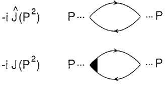
Figure 1: (a) The basic vacuum polarization diagram of the NJL model is shown. The lines represent a constituent quark and antiquark of mass $m(\rho_{q})$.
(b) The filled region represents a confinement vertex used for calculations made for $\rho\leq\rho_{c}$ [9].

In forming the imaginary parts of the vacuum polarization functions, the quark and antiquark go on mass shell, so that we have $\vec{k}^{2}=(P^{0})^{2}/4-m^{2}(\rho)$. It is easy to see that there is a minimum value of $|\vec{k}|=p_{F}$, where $p_{F}$ is the Fermi momentum of either the up or down ideal quark gases. For smaller values of $|\vec{k}|$ the excitation is “blocked” by the Pauli Principle. Thus, we see that in calculating the imaginary part of a vacuum polarization function, one obtains nonzero values above a minimum value of $P^{0}$, $(P^{0})_{min}^{2}=4(p_{F}^{2}+m^{2}(\rho))$, where $p_{F}$ is related to the quark density by the expression $p_{F}^{3}=(3\pi^{2}/2N_{c})\rho_{q}$, given earlier.

We now consider the imaginary part of the vacuum polarization function corresponding to scalar currents. We find in the case an up (or down) quark is excited

$$\mbox{Im}J^{S}(P^{2})=N_{c}\frac{P_{0}^{2}}{4\pi}\left(1-\frac{4m_{u}^{2}(\rho)}{P_{0}^{2}}\right)^{3/2}e^{-\vec{k}^{2}/\alpha^{2}}\theta[P_{0}-4(p_{F}^{2}+m_{u}^{2}(\rho))]\,.$$ (2.2)

This expression contains a factor of 2 arising from the flavor trace. Here $\vec{k}^{2}=P_{0}^{2}/4-m_{u}^{2}(\rho)$ appears in the Gaussian regulator. (We have used Gaussian regulators for most of our calculations made using the NJL model. The value of $\alpha=0.605$ GeV yields results that are similar to those obtained with the sharp three-momentum cutoff parameter $\Lambda=0.631$ GeV.) For pseudoscalar mesons, we may use Eq. (2.2) with the phase-factor exponent of 3/2 replace by 1/2 when the constituent mass is small [10]. The real parts of the vacuum polarization functions are obtained by means of a dispersion relation.

We now consider the calculation of density-dependent hadronic current correlation functions. The general form of the correlator is a transform of a time-ordered product of currents,

$$C(P^{2},\rho)=i\int d^{4}xe^{\,ip\cdot x}<<\mbox{T}(j(x)j(0)>>\,,$$ (2.3)

where the double bracket is a reminder that we are considering the finite density case.

For the study of pseudoscalar states, we may consider currents of the form $j_{P,\,i}(x)=\bar{q}(x)i\gamma_{5}\lambda^{i}q(x)$ where, in the case of the $\pi$ mesons, $i=1,2,$ and 3. For the study of pseudoscalar-isoscalar mesons, we again introduce $j_{P,\,i}(x)=\bar{q}(x)\lambda^{i}q(x)$, but here $i=0$ for the flavor-singlet current and $i=8$ for the flavor-octet current.

In the case of the $\pi$ mesons, the correlator may be expressed in terms of the basic vacuum polarization function of the NJL model, $J_{P}(P^{2},\rho)$. Thus,

$$C_{\pi}(P^{2},\rho)=J_{P}(P^{2},\rho)\frac{1}{1-G_{\pi}(\rho)J_{P}(P^{2},\rho)}\,,$$ (2.4)

where $G_{\pi}(\rho)$ is the coupling constant appropriate for our study of the $\pi$ mesons. (We have found $G_{\pi}(0)=13.49$ GeV^-2 by fitting the pion mass in a calculation made at $\rho=0$.)

For a study of the correlators related to the $\rho$ meson, we introduce conserved vector currents $j_{\mu,\,i}(x)=\bar{q}(x)\gamma_{\mu}\lambda_{i}q(x)$ with $i=1,2$ and 3. In this case we define

$$J_{\rho}^{\mu\nu}(P^{2},\rho)=\left(g\,{}^{\mu\nu}-\frac{P\,{}^{\mu}P\,{}^{\nu}}{P^{2}}\right)J_{\rho}(P^{2},\rho)\,,$$ (2.5)

taking into account the fact that the current $j_{\mu,\,i}(x)$ is conserved. We may then use the fact that

$$J_{\rho}(P^{2},\rho) = \frac{1}{3}g_{\mu\nu}J_{\rho}^{\mu\nu}(P^{2},\rho)$$ (2.6)

$$= \frac{2N_{c}}{3}\left[\frac{P_{0}^{2}+2m_{u}^{2}(\rho)}{4\pi}\right]\left(1-\frac{4m_{u}^{2}(\rho)}{P_{0}^{2}}\right)^{1/2}e^{-\vec{k}\,{}^{2}/\alpha^{2}}\theta[P_{0}^{2}-4(p_{F}^{2}+m_{u}^{2}(\rho))]$$ (2.7)

$$\simeq \frac{2}{3}J_{\pi}(P^{2},\rho)$$ (2.8)

and write the approximate expression

$$\mbox{Im}J_{\rho}(P^{2},\rho)\simeq\frac{2}{3}\frac{N_{c}P_{0}^{2}}{4\pi}\left(1-\frac{4m_{u}^{2}(\rho)}{P_{0}^{2}}\right)^{1/2}e^{-\vec{k}\,{}^{2}/\alpha^{2}}\theta[P_{0}^{2}-4(p_{F}^{2}+m_{u}^{2}(\rho))]$$ (2.9)

for the vacuum polarization function of the vector-isovector currents. Here $\vec{k}^{2}=P_{0}^{2}/4-m_{u}^{2}(\rho)$ appears in the Gaussian regulator. Thus, we define

$$C_{\rho}(P^{2})=J_{\rho}(P^{2})\left[\frac{1}{1-G_{V}(\rho)J_{\rho}(P^{2})}\right]\,,$$ (2.10)

where we have suppressed reference to the density dependence of the correlator and the vacuum polarization function. We have used $G_{V}(\rho)=G_{V}[1-0.17\rho/\rho_{c}]$ with $G_{V}=11.46$ GeV^-2 for the calculators reported here.

The calculation of the correlator for scalar-isoscalar states is more complex, since there are both flavor-singlet and flavor-octet states to consider. We may define polarization functions for $u$, $d$ and $s$ quarks: $J_{u}(P^{2},\rho)$, $J_{d}(P^{2},\rho)$ and $J_{s}(P^{2},\rho)$. These functions do not contain the factor of 2 arising from the flavor trace that was introduced when calculating $\mbox{Im}J_{\pi}(P^{2},\rho)$, $\mbox{Im}J^{S}(P^{2},\rho)$ and $\mbox{Im}J_{\rho}(P^{2},\rho)$ earlier in this section.

In terms of these polarization functions we may then define

$$J_{00}(p^{2},\rho)=\frac{2}{3}[J_{u}(p^{2},\rho)+J_{d}(p^{2},\rho)+J_{s}(p^{2},\rho)]\,,$$ (2.11)

$$J_{08}(p^{2},\rho)=\frac{\sqrt{2}}{3}[J_{u}(p^{2},\rho)+J_{d}(p^{2},\rho)-2J_{s}(p^{2},\rho)]\,,$$ (2.12)

and

$$J_{88}(p^{2},\rho)=\frac{1}{3}[J_{u}(p^{2},\rho)+J_{d}(p^{2},\rho)+4J_{s}(p^{2},\rho)]\,.$$ (2.13)

We also introduce the matrices

$$J(p^{2},\rho)=\left[\begin{array}[]{cc}J_{00}(p^{2},\rho)&J_{08}(p^{2},\rho)\\ J_{80}(p^{2},\rho)&J_{88}(p^{2},\rho)\end{array}\right]\,,$$ (2.16)

$$G(\rho)=\left[\begin{array}[]{cc}G_{00}(\rho)&G_{08}(\rho)\\ G_{80}(\rho)&G_{88}(\rho)\end{array}\right]\,,$$ (2.19)

$$C(p^{2},\rho)=\left[\begin{array}[]{cc}C_{00}(p^{2},\rho)&C_{08}(p^{2},\rho)\\ C_{80}(p^{2},\rho)&C_{88}(p^{2},\rho)\end{array}\right]\,,$$ (2.22)

and write the matrix relation

$$C(p^{2},\rho)=J(p^{2},\rho)[1-G(\rho)J(p^{2},\rho)]^{-1}\,.$$ (2.23)

III results of numerical calculations of pseudoscalar and vector hadronic current correlation functions, $C_{\pi}(P^{2})$ and $C_{\rho}(P^{2})$

In Fig. 2 we present values calculated for $\mbox{Im}C_{\pi}(P^{2})$ for $\rho/\rho_{c}=1.2$, 2.0, 3.0, 4.0 and 5.88. The threshold for each curve is given by $(P^{0})_{min}^{2}=4(p_{F}^{2}+m_{u}^{2}(\rho_{q}))$. If $\rho_{c}=2.25\rho_{NM}$, we have

$$p_{F}=\left(\frac{2.25}{N_{c}}\frac{\rho}{\rho_{c}}\right)^{1/3}k_{F}\,,$$ (3.1)

where $k_{F}$ is the Fermi momentum of nuclear matter, $k_{F}=0.286$ GeV. Thus, when $\rho/\rho_{c}=5.88$, we find $p_{F}=0.439$ GeV, which is less than the standard three-dimensional (sharp) cutoff of $\Lambda=0.631$ GeV that is often used for the NJL model. It is seen from the figure that there are significant nonperturbative effects, except at $\rho/\rho_{c}=5.88$, where $\mbox{Im}C_{\pi}(P^{2})=\mbox{Im}J_{\pi}(P^{2})$. The last result follows, since $G_{\pi}(\rho)=0$ for $\rho/\rho_{c}=5.88$.

Figure 2: The figure presents values of $\mbox{Im}C_{\pi}(P^{2})$ for various values of $\rho/\rho_{c}$. Here, $\rho/\rho_{c}=1.2$ [solid line], 2.0 [dashed line], 3.0 [dotted line], 4.0 [dashed-dotted line] and 5.88 [dashed-(double)dotted line]. We have used $G_{\pi}=13.51$ GeV^-2.

In Fig. 3 we show the results of a similar calculation of $\mbox{Im}C_{\rho}(P^{2})$. Here the thresholds for the various curves are the same as those seen in Fig. 2.

Figure 3: The figure shown the values of $\mbox{Im}C_{\rho}(P^{2})$. [See the caption of Fig. 2.] Here we have used $G_{V}=11.46$ GeV^-2.

IV results of numerical calculation of scalar and pseudo-scalar correlators $C_{f_{0}88}(P^{2})$ and $C_{\eta 88}(P^{2})$

In the case of the correlator of pseudoscalar-isoscalar currents, the components $C_{\eta 00}(P^{2})$, $C_{\eta 08}(P^{2})=C_{\eta 80}(P^{2})$ and $C_{\eta 88}(P^{2})$ are all important. We choose to show $\mbox{Im}C_{\eta 88}(P^{2})$ in Fig. 4 for the values of $\rho/\rho_{c}=$ 1.5, 2.0, 3.0, 4.0 and 5.88. The resonant structures have rather small widths when compared to the features seen in Fig. 2 and 3. It is also worth noting that each curve has two thresholds, one corresponding to $m_{u}(\rho)$ and the other corresponding to $m_{s}(\rho)$. Thus, we have $(P^{0})_{min}^{2}=4[p_{F}^{2}+m_{u}^{2}(\rho)]$ or $(P^{0})_{min}^{2}=4[p_{F}^{2}+m_{s}^{2}(\rho)]$.

Figure 4: The figure shows the values calculated for the imaginary part of the correlator of pseudoscalar, flavor-octet currents $\mbox{Im}C_{\eta 88}(P^{2})$. Here, $\rho/\rho_{c}=1.5$ [solid line], 2.0 [dashed line], 3.0 [dotted line], 4.0 [dashed-dotted line], 5.0 [dashed-(double)dotted line], and 5.88 [short dashed line].

Similar remarks pertain for the scalar current correlators, $C_{f_{0}00}(P^{2})$, $C_{f_{0}08}(P^{2})=C_{f_{0}80}(P^{2})$ and $C_{f_{0}88}(P^{2})$. The values of $\mbox{Im}C_{f_{0}88}(P^{2})$ are shown in Fig. 5 for various values of $\rho/\rho_{c}$. Note that the resonances seen in that figure are quite narrow. That is probably due to the different phase space behavior for the $f_{0}$ ($p$-wave) and $\eta$ ($s$-wave).

Figure 5: The values of the imaginary part of the correlator of scalar, flavor-octet hadronic currents, $\mbox{Im}C_{f_{0}88}(P^{2})$ is shown. [See caption of Fig. 4.]

V results of numerical calculations with density-dependent and density-independent NJL coupling constants

In this section we are interested in presenting some evidence for the density-dependent coupling constants used in our work [9]. (As noted earlier, the argument is more easily made when we introduce temperature-dependent coupling constants, since much more is known concerning QCD thermodynamics at finite temperature than at finite density.) In the case of finite density, we have assumed that the system is weakly interacting at $\rho=5.88\rho_{c}$ with $\rho_{c}=2.25\rho_{NM}$. (Other values for $\rho_{c}$ could be used, but here we will continue to explore the consequences of the choice made in our earlier work [9].) In Fig. 6 we compare the results of our model for $\mbox{Im}C_{\pi}(P^{2})$ at $\rho/\rho_{c}=5.88$ with the results obtained when we use a constant value for $G_{\pi}$. As seen in the figure, there is about a factor of 3 difference in the result of the two calculations. The difference in the two calculated results for $\mbox{Im}C_{\rho}(P^{2})$ seen in Fig. 7 is not quite as marked as that seen in Fig. 6, but is still significant.

Figure 6: The solid line shows the values of $\mbox{Im}C_{\pi}(P^{2})$ for the case of density-independent NJL coupling constants. The dashed-(double)dotted line represents $\mbox{Im}C_{\pi}(P^{2})$ calculated with the density-dependent coupling constants $G_{\pi}(\rho)=G_{\pi}[1-0.17\rho/\rho_{c}]$ for $\rho/\rho_{c}=5.88$.

Figure 7: The solid line shows the values of $\mbox{Im}C_{\rho}(P^{2})$ for the case of density-independent NJL coupling constants. The dashed-(double)dotted line represents $\mbox{Im}C_{\rho}(P^{2})$ calculated with the density-dependent coupling constants $G_{V}(\rho)=G_{V}[1-0.17\rho/\rho_{c}]$ for $\rho/\rho_{c}=5.88$.

In Fig. 8 we compare the results for $\mbox{Im}C_{\eta 88}(P^{2})$ at $\rho/\rho_{c}=5.88$ for the two methods of calculation. A rather dramatic difference is seen in Fig. 8, where we see that the calculation with constant values of $G_{00}^{P}$, $G_{08}^{P}$ and $G_{88}^{P}$ leads to a resonance at $P^{2}=1.53$ GeV². In Fig. 9 we show similar results for $\mbox{Im}C_{f_{0}88}(P^{2})$ with a resonance at $P^{2}=1.58$ GeV² in the case that constant values of $G_{00}^{P}$, $G_{08}^{P}$ and $G_{88}^{P}$ are used.

Figure 8: The figure shows $\mbox{Im}C_{\eta 88}(P^{2})$ calculated for $\rho/\rho_{c}=5.88$. The dashed-(double)dotted line is the result of using our density-dependent coupling parameters, while the solid line is the result when density-independent coupling parameters are used.

Figure 9: The figure shows $\mbox{Im}C_{f_{0}88}(P^{2})$

calculated for $\rho/\rho_{c}=5.88$. [See the caption of Fig. 8.]

VI discussion

In this work we have assumed that deconfinement takes place at $\rho_{c}=2.25\rho_{NM}$ and that the quark gluon plasma is weakly interacting at $\rho=5.88\rho_{c}=13.2\rho_{NM}$. This particular model was explored in Ref. [9] where we calculated the masses of several mesons and their radial excitations for various matter densities, $\rho\leq\rho_{c}$, making use of our generalized NJL model with confinement. In the present work we have put forth some evidence that the NJL coupling constants should be density dependent to obtain a consistent formalism. We may consider what results would be obtained if we used a larger value of the density for the confinement-deconfinement transition. We have investigated the values of $\rho_{c}=3.0\rho_{NM}$, $\rho_{c}=4.0\rho_{NM}$ and $\rho_{c}=5.0\rho_{NM}$ and in each case have assumed that the quark-gluon plasma is weakly interacting for $\rho=6.0\rho_{c}$. (We should note that, if $\rho_{c}$ is made large, the value calculated for $p_{F}$ will become larger than the value of the three-momentum NJL cutoff, $\Lambda=0.631$ GeV, that is often used. However, our computer code still provides results under that circumstance, since we use a Gaussian regulator.) It is found in all the calculations made at the values of $\rho$ for which we have assumed the system to be weakly interacting, that the values of the correlators calculated with constant values of the coupling constants differ significantly from the results obtained with the density-dependent coupling constants. We suggest that this matter should be resolved before we undertake studies of diquark condensation at high densities and related matters.

One characteristic of our calculation of hadronic current correlators at finite temperature and finite density in the deconfined phase is the appearance of complex resonance structure in some cases. That feature is in general agreement with the observation made in Ref. [26] “…that the correlators possess a nontrivial structure in the deconfined phase.” Meson correlators were studied in finite temperature lattice QCD in Ref. [27], in which the authors state, “…Below $T_{c}$ we observe little change in the meson properties as compared with $T=0$. Above $T_{c}$ we observe new features: chiral symmetry restoration and signals of plasma formation, but also an indication of persisting “mesonic” (metastable) states and different temporal and spacial masses in the mesonic channels. This suggests a complex picture of QGP in the region (1-1.5)$T_{c}$”.

References

- (1) T. Renk, R. A. Schneider, and W. Weise, Nucl. Phys. A 699, 16 (2002).
- (2) C. R. Allton, S. Ejiri, S. J. Hands, O. Kaczmarek, F. Karsch, E. Laermann, Ch. Schmidt, and L. Scorzato, Phys. Rev. D (to be published), hep-lat/0204010.
- (3) S. Ejiri, C. R. Allton, S. J. Hands, O. Kaczmarek, F. Karsch, E. Laermann, and L. Scorzato, Nucl. Phys. B (Proc. Suppl.) 106, 459 (2002).
- (4) F. Karsch, Lect. Notes Phys. 583, 209 (2002).
- (5) F. Karsch, Nucl. Phys. B (Proc. Suppl.) 83, 14 (2000).
- (6) J. Engels, O. Kaczmarek, F. Karsch and E. Laermann, Nucl. Phys. B 558, 307 (1999).
- (7) Z. Fodor and S. D. Katz, hep-lat/0204029; Nucl. Phys. B (Proc. Suppl.) 106, 441 (2002) [hep-lat/0106002]; Phys. Lett. B 534, 87 (2002).
- (8) Hu Li and C. M. Shakin, hep-ph/0209136.
- (9) Hu Li and C. M. Shakin, Phys. Rev. D 66, 074016 (2002).
- (10) Hu Li and C. M. Shakin, hep-ph/0209258.
- (11) Bing He, Hu Li, C. M. Shakin, and Qing Sun, hep-ph/0210387.
- (12) For reviews, see K. Rajagopal and F. Wilcek, in At the Frontier of Particle Physics/Handbook of QCD, M. Shifman ed. (World Scientific, Singapore 2001); M. Alford, Annu. Rev. Nucl. Part. Sci. 51, 131 (2001).
- (13) M. Alford, R. Rajagopal and F. Wilcek, Phys. Lett. B 422 , 247 (1998).
- (14) R. Rapp, T. Schfer, E. V. Shuryak and M. Velkovsky, Phys. Rev. Lett. 81 , 53 (1998).
- (15) M. Alford, J. Berges and K. Rajagopal, Nucl. Phys. B 558 , 219 (1999).
- (16) M. Le Bellac, Thermal Field Theory (Cambridge Univ. Press, Cambridge, 1996)-See Fig. 1.3.
- (17) T. Hatsuda and T. Kunihiro, Phys. Rep. 247 , 221 (1994).
- (18) S. P. Klevansky, Rev. Mod. Phys. 64 , 649 (1992).
- (19) U. Vogl and W. Weise, Prog. Part. Nucl. Phys. 27 , 195 (1991).
- (20) C. M. Shakin and Huangsheng Wang, Phys. Rev. D 65 , 094003 (2002).
- (21) C. M. Shakin and Huangsheng Wang, Phys. Rev. D 64 , 094020 (2001).
- (22) C. M. Shakin and Huangsheng Wang, Phys. Rev. D 63 , 074017 (2001).
- (23) L. S. Celenza, Huangsheng Wang, and C. M. Shakin, Phys. Rev. C 63 , 025209 (2001).
- (24) C. M. Shakin and Huangsheng Wang, Phys. Rev. D 63 , 014019 (2000).
- (25) L. S. Celenza, Hu Li, C. M. Shakin, and Qing Sun, Phys. Rev. D 66, 054010 (2002).
- (26) T. Umeda, K. Nomura and H. Matsufuru, hep-lat/0211003.
- (27) Ph. de Forcrand, M. GarciaPerez, T. Hashimoto, S. Hioki, H. Matsufuru, O. Miyamura, A. Nakamura, I. O. Stamatescu, T. Takaishi and T. Umeda, Phys. Rev. D 63, 054501 (2001).