Radiative corrections to low energy neutrino reactions

Abstract

We show that the radiative corrections to charged current (CC) nuclear reactions with an electron(positron) in the final state are described by a universal function. The consistency of our treatment of the radiative corrections with the procedure used to extract the value of the axial coupling constant $g_{A}$ is discussed. To illustrate we apply our results to (anti)neutrino deuterium disintegration and to $pp$ fusion in the sun. The limit of vanishing electron mass is considered, and a simple formula valid for $E_{obs}\mathrel{\;{\hbox{\raise 1.50696pt\hbox{$>$}}\kern-3.8889pt\kern-3.8889pt\hbox{\lower 2.79857pt\hbox{$\sim$}}}\;}1$ MeV is obtained. The size of the nuclear structure-dependent effects is also discussed. Finally, we consider CC transitions with an electron(positron) in the initial state and discuss some applications to electron capture reactions.

PACS number(s): 13.10.+q, 13.15.+g, 25.30.Pt

I Introduction

The physics of neutrino flavor oscillations has entered a new era. There is now a consensus that the observation of the atmospheric neutrinos [1] can be interpreted as an evidence that muon neutrinos born in the atmosphere oscillate into tau neutrinos. At the same time, numerous measurements of solar electron neutrino fluxes have been pointing toward neutrino oscillations ever since the Homestake experiment [2]. The evidence for oscillation of solar neutrinos has been strengthened recently with the results from Sudbury Neutrino Observatory (SNO) [3, 4] that are independent of the solar model (SSM). With the evidence for oscillations at hand, the accurate determination of the neutrino masses and flavor mixing angles is the most important task for neutrino physics at present. Carrying out the above program requires accurate knowledge of the cross sections of the reactions used for neutrino detection, and the Standard Model (SM) radiative corrections, which typically shift the leading (tree) order values by 3-4%, must be taken into account.

Complete one-loop SM radiative corrections to the CC and neutral current (NC) deuteron disintegration by electron neutrinos used in SNO measurements have been calculated in Refs. [5, 6]. We have shown in Ref. [5] that while the differential CC cross section depends on the actual detector properties (e.g. on the bremsstrahlung detection threshold $E_{\gamma}^{min}$) the total cross section is a detector-independent quantity as long as the final state electron is always detected, i.e., the total number of the neutrino interactions is determined. In the simple case when $E_{\gamma}^{min}\rightarrow 0$ one finds:

$$d\sigma_{CC}(E_{obs})=d\sigma^{\rm Tree}_{CC}(E_{obs})\left(1+{\alpha\over\pi}g(E_{obs})\right)~{},$$ (1)

where $d\sigma^{\rm Tree}_{CC}(E_{obs})$ and $d\sigma_{CC}(E_{obs})$ are, respectively, the leading and the next to leading order in $\alpha$ differential cross sections, $E_{obs}$ is the energy observed in the detector (charged lepton energy plus possible bremsstrahlung photon energy), and $g(E_{obs})$ is given by the Eq. (5) below. It is understood that the cross section $d\sigma^{\rm Tree}_{CC}(E_{obs})$ includes the Fermi function $F(Z,A,E_{obs})$ to account for the distortion of the final state electron wavefunction by the Coulomb field of the final nucleus (see e.g. Ref. [7]). While a similar approach to the treatment of radiative corrections has long been used in the analysis of nuclear beta decay [8, 9], here we extend it to a wide class of reactions involving neutrinos, and formulate the conditions for its applicability . Specifically, we generalize the results of Ref. [5] and analyze the following four features of the radiative corrections.

1. Universality. The function $g(E)$ is universal for a class of nuclear reactions involving neutrinos. In particular, it can be used to evaluate the radiative corrections to the total cross-sections of reactions that have an electron (positron) in the final state. It is applicable not only to neutron and nuclear $\beta$-decays, but also to the antineutrino capture reactions, low energy CC neutrino-nucleus disintegration, nuclear fusion reactions accompanied by the electron(positron) emission, etc. For illustration we consider the following CC processes involving two nucleon systems:

$$\nu_{e}+d \rightarrow p+p+e^{-}~{},$$ (2)

$${\bar{\nu}}_{e}+d \rightarrow n+n+e^{+}~{},$$ (3)

$$p+p \rightarrow d+e^{+}+\nu_{e}~{}.$$ (4)

For reactions where the electron spectrum is narrow (precise conditions are given in Section II) we provide a simple and accurate way to calculate the correction to the total cross section without the complicated integration over the outgoing electron or positron spectrum.

In order to demonstrate one of the possible applications of our results, note that the last reaction in Eq. (2) is the main reaction for the $pp$ chain that powers the Sun (see e.g. Ref. [10]). The total rate of this reaction is, therefore, constrained by the known solar luminosity. That rate, together with the cross-section for the $pp$ reaction, is used to calibrate the SSM and to predict many other quantities, in particular the flux of the ⁸B neutrinos studied at SNO. Below we show that a proper treatment of the radiative corrections to $S_{pp}$, the S-factor for the $pp$ reaction, lowers the SSM prediction to $\Phi(^{8}{\rm B})$ by about 0.6% relative to the currently accepted value [11].

2. Axial coupling constant $g_{A}$. Since the reactions in Eq.(2) are dominated by the nuclear axial current, it is important to use a procedure consistent with the definition of the axial coupling constant $g_{A}$. We briefly discuss the conventional definition of $g_{A}$ based on the value extracted from neutron decay and give a prescription for evaluation of the radiative corrections consistent with that definition. This issue has been discussed in the literature (see e.g. Ref. [13]) but we feel that it is sufficiently important to reiterate here.

3. Nuclear structure-dependent effects. In deriving universality properties of the radiative corrections we work in the “one-body” approximation (in analogy to the early applications to the nuclear beta decay). Namely, we evaluate the radiative correction to the CC reaction on a single nucleon, and then use it to compute the correction to the reaction of interest. Effectively, only the corrections of the type shown in Fig.1(a) are included in such a calculation. Nuclear structure-dependent many-body corrections of the type shown in Fig.1(b) are thus neglected. We show that a comparison of such corrections to analogous effects contributing to superallowed Fermi transitions in nuclei suggests that they enter at 0.1% level. As we discuss in Section V, however, this estimate of universality-breaking contributions is not airtight, and a detailed computation is needed to obtain precise numbers.

4. Collinear singularities. We study the behavior of the radiative corrections in the limit $m_{e}\rightarrow 0$, where $m_{e}$ is the electron mass. Separate contributions to the corrections are singular in this limit, and until now it has not been explicitly shown in the literature how the singularities cancel when all contributions are added. Such cancellation must take place according to the well-known Kinoshita-Lee-Nauenberg (KLN) theorem[14], and in Section VI we show how this happens. As a corollary we obtain a simple expression for $g(E)$ valid for $E\gg m_{e}$. In practice, radiative corrections evaluated according to this simple expression are accurate to about 0.1% for energies above 1 MeV.

Although these four topics constitute the main focus of our study, we also discuss processes, such as capture reactions, involving charged leptons in the initial state. In this case, the radiative corrections do not display the same kind of universality applicable to the reactions in Eq. (2). Nevertheless, the treatment of the two cases is sufficiently similar that we feel a brief discussion – given at the end of the paper – is warranted.

II Universality of the radiative corrections to reactions with the electron/positron in the final state

We begin with the first reaction in Eq.(2). As was shown in Ref. [5], the total cross section is independent of the photon detection threshold $E_{\gamma}^{min}$. In the limit $E_{\gamma}^{min}\to 0$ the function $g(E)$ in Eq.(1) has two parts:

$$g(E)=g_{v}(E)+g_{b}(E)~{}.$$ (5)

Here, $g_{v}(E)$ (for the virtual part) and $g_{b}(E)$ (for the bremsstrahlung part) are given by the following lengthy expressions (the cutoff parameter $\Lambda$ that appears in Ref. [5, 6] is set equal to the proton mass):

$$g_{v}(E) = 2\ln\left({M_{Z}\over M_{p}}\right)+\frac{3}{2}~{}{\rm ln}\left(\frac{M_{p}}{m_{e}}\right)$$ (6)

$$+ 2\ln\left({E-m_{e}\over m_{e}}\right)\left({1\over 2\beta(E)}\ln\left({1+\beta(E)\over 1-\beta(E)}\right)-1\right)$$ (7)

$$+ {3\over 4}+{\cal A}(\beta(E))-0.57~{},$$ (8)

$${\cal A}(\beta) = \frac{1}{2}\beta~{}{\rm ln}\left(\frac{1+\beta}{1-\beta}\right)-1-\frac{1}{\beta}\left[\frac{1}{2}{\rm ln}\left(\frac{1+\beta}{1-\beta}\right)\right]^{2}+\frac{1}{\beta}L\left(\frac{2\beta}{1+\beta}\right)~{}.$$ (9)

and

$$g_{b}(E) = {\cal C}(\beta(E))+{1\over 2E^{2}\beta(E)}\Biggl{(}\int_{m_{e}}^{E}(E-x)\ln\left({1+\beta(x)\over 1-\beta(x)}\right)dx$$ (11)

$$+ 4E\int_{m_{e}}^{E}{x\beta(x)F(x)-E\beta(E)F(E)\over E-x}dx\Biggr{)}~{},$$ (12)

$$F(E) = {1\over 2\beta(E)}\ln\left({1+\beta(E)\over 1-\beta(E)}\right)-1~{},$$ (13)

$${\cal C}(\beta) = 2\ln(2)\left[\frac{1}{2\beta}\ln\left(\frac{1+\beta}{1-\beta}\right)-1\right]+1+\frac{1}{4\beta}\ln\left(\frac{1+\beta}{1-\beta}\right)$$ (15)

$$\times\left[2+\ln\left({{1-\beta^{2}}\over 4}\right)\right]+{1\over{\beta}}\left[{L(\beta)-L(-\beta)}\right]$$

$$+ {1\over 2\beta}\left({L\left({{1-\beta}\over{2}}\right)-L\left({{1+\beta}\over{2}}\right)}\right)~{}.$$ (16)

In the above equations, $m_{e}$ is the electron mass and:

$$\beta(E) = {\sqrt{E^{2}-m_{e}^{2}}\over|E|}~{},$$ (17)

$$L(\beta) = \int_{0}^{\beta}{{\ln(|1-x|)}\over x}dx~{}{\stackrel{{\scriptstyle|\beta|\leq 1}}{{=}}}~{}-\sum_{k=1}^{\infty}\frac{\beta^{k}}{k^{2}}~{}.$$ (18)

The closed form for the integrals appearing in Eq. (11) is given in the appendix. Although $g(E_{obs})$ in general depends on the value of the cutoff parameter $\Lambda$, the choice of $\Lambda$ affects only the constant, energy independent part of $g_{v}(E_{obs})$. We chose $\Lambda=M_{p}$ and adjusted the constant (-0.57) in the Eq.(6) so that the result matches with the corresponding expression derived by Sirlin in Ref. [9] based on current algebra (the same approach was chosen in Ref. [6]). The dominant uncertainty in $g(E_{obs})$ is associated with the value of the matching constant and is briefly discussed after Eq. (20).

It is remarkable that $g(E_{obs})$ is a function of a single parameter – the observed energy $E_{obs}$ – and does not depend on the electron and photon energies separately. Moreover, formulas Eq.(6) and Eq.(11) make no reference to the parameters that describe the leading-order differential cross section, such as $pp$ scattering length or the effective range (see e.g. Ref. [15] for definitions). It is, therefore, reasonable to ask whether $g(E_{obs})$ is a universal function that describes the radiative corrections to a whole class of processes in the limit $E_{\gamma}^{min}\rightarrow 0$. Below we show that this is indeed the case.

Consider first, in the one-nucleon approximation, contributions from virtual photon exchanges. As pointed out in Refs. [5, 6], it is convenient to split these contribution into two pieces: with $\kappa<\Lambda$ and with $\kappa\geq\Lambda$, where $\kappa$ is the scale for the virtual photon momenta and $\Lambda$ is a cutoff, taken to be of the order of 1 GeV. Contributions with $\kappa\geq\Lambda$, usually called “inner” radiative corrections, are combined with the $Z^{0}$ boson exchange box graphs to produce an energy-independent contribution to $g(E_{obs})$ [6]:

$$g_{v}(E_{obs})^{\kappa\geq\Lambda}=2\ln\left(M_{Z}\over\Lambda\right)~{}.$$ (19)

This contribution is obviously common to all reactions in Eq.(2) since it contains no parameters that distinguish between them.

The piece with $\kappa<\Lambda$ is more complicated. The virtual exchanges of a low energy photon for all three reactions Eq.(2) are shown in Fig.2. The correction to Fig.2(a) is [5, 6]:

$$g_{v}(E_{obs})^{\kappa<\Lambda} = 3\ln\left({\Lambda\over M_{p}}\right)+{3\over 2}\ln\left({M_{p}\over m_{e}}\right)+{3\over 4}+{\cal A}(\beta(E_{obs}))$$ (20)

$$+ 2\ln\left({\lambda\over m_{e}}\right)\left[{1\over 2\beta(E_{obs})}\ln\left({1+\beta(E_{obs})\over 1-\beta(E_{obs})}\right)-1\right]-0.57+\delta{\widetilde{C}}(\Lambda)~{},$$ (21)

where $\lambda$ is the “photon mass” used as the infrared regulator and ${\cal A}(\beta)$ is given in Eq. (6). The parameter $\delta{\widetilde{C}}$ represents a matching constant arising from presently incalculable non-perturbative QCD effects. Its $\Lambda$-dependence must cancel the corresponding dependence in $g(E_{obs})$. Unfortunately, no existing calculation of $\delta{\widetilde{C}}$ has demonstrated this cancellation explicitly. In addition, $\delta{\widetilde{C}}$ will contain $\Lambda$-independent terms that depend on the light-quark masses, $\Lambda_{\rm QCD}$, etc.. A complete, first principles computation of these contributions has yet to be performed, so we must rely on models. Thus, in practical calculations we set this constant to zero for $\Lambda=M_{p}$ to match the model results of Refs. [9, 16, 17]. The uncertainty in $g_{v}(E)$ associated with $\delta{\widetilde{C}}$ is estimated in Ref. [17] to be about 0.08%.

Even though the virtual momenta in Figs.2(b,c) are different from those on Fig.2(a) their contributions are also given by the Eq.(20). The easiest way to see it is as follows. Consider Fig.2(b) first. This graph can be obtained from Fig. 2(a) through time reversal followed by replacements $e^{-}({\rm initial})\rightarrow e^{+}({\rm final})$ and $\nu_{e}({\rm final})\rightarrow{\bar{\nu}}_{e}({\rm initial})$. Since time reversal is an exact symmetry of QED, the scattering amplitude is unchanged up to an overall phase. The result of replacements of the particles with antiparticles can be found by utilizing crossing symmetry. However, the replacement $p_{e}\rightarrow-p_{e}$ does not change $\beta(E_{e})$ (see Eq.(17) for the definition). Since Eq. (20) depends on the electron momenta only through $\beta(E_{e})$ it is obviously invariant. Hence, Eq. (20) is applicable to the second process in Eq.(2). The validity of the Eq. (20) for the third process in Eq.(2) trivially follows from the fact that Eq. (20) is independent of the neutrino 4-momentum. Indeed, going from Fig.2(b) to Fig.2(c), which is accomplished by replacing the antineutrino with the neutrino and changing the sign of its 4-momentum, leaves the Eq. (20) invariant.

The bremsstrahlung contributions are also identical for all three reactions under consideration [Eq.(2)]. In particular, for these reactions, only the bremsstrahlung from the charged lepton is important since all other charged particles are heavy. Therefore, for each of the processes under consideration there is only one bremsstrahlung diagram of the type shown in Fig.3. The amplitude for this graph has the form:

$${\cal M}_{\gamma}\sim{eG_{F}\over\sqrt{2}}\epsilon_{\nu}L_{\gamma}^{\mu\nu}H_{\mu}(q)~{},$$ (22)

where $e$ is the electron charge, $\epsilon_{\nu}$ is the photon polarization, and $L_{\gamma}^{\mu\nu}$ and $H_{\mu}(q)$ represent, respectively, the leptonic and the hadronic contributions to the process:

$$H_{\mu}(q) = \int e^{iq\cdot x}\langle f_{N}|\sum_{m=1}^{A}J_{\mu}^{m}(x)|i_{N}\rangle d^{4}x$$ (23)

$$L_{\gamma}^{\mu\nu} = \int e^{-iq\cdot x-ik\cdot y}\langle f_{L}|T\{J^{\mu}(x)J_{\rm EM}^{\nu}(y)\}|i_{L}\rangle d^{4}xd^{4}y~{}.$$ (24)

Here $i_{N,L}$ and $f_{N,L}$ are, respectively, the initial and the final states of the nuclear and the leptonic parts of the process, $J_{\mu}$ is the relevant charged current, $J_{\rm EM}^{\nu}$ is the electromagnetic current, and $k$ is the momentum of the emitted photon. The summation index $m$ in the hadronic matrix element runs over all nucleons in the nucleus. The dependence of $H_{\mu}$ on the momentum transfer $q$ is explicitly shown. In the long wavelength approximation, valid for low neutrino energies, one can neglect the dependence of $H_{\mu}$ on the spatial components of $q$. On the other hand, the dependence of $H_{\mu}$ on the time component of $q$ could be crucial. Indeed, energy conservation implies that the initial $E_{i}$ and final $E_{f}$ energies of the hadronic system obey the relation $E_{f}=E_{i}+q^{0}$. Clearly, the nuclear matrix element depends sensitively on the value of $E_{f}$, the excitation energy of the final state. In the case of CC neutrino deuteron disintegration, for example, changing $E_{f}$ causes a dramatic change in the shape of the final state $pp$ wavefunction and the corresponding change in the size of the nuclear matrix element[5].

With these consideration in mind, and using the results of Ref. [5, 6], it is easy to show that the square of the matrix element Eq.(22) averaged over the initial and summed over the final spins has the form

$$\langle|{\cal M}_{\gamma}(E_{\nu},E_{e},E_{\gamma},x)|^{2}\rangle = {\alpha\over\pi}\langle|{\cal M}_{0}(E_{\nu},E_{obs})|^{2}\rangle\times{E_{e}\over E_{obs}}F(E_{\gamma},E_{e},x)~{},$$ (25)

$$q^{0} \equiv \pm E_{\nu}-E_{e}-E_{\gamma}=\pm E_{\nu}-E_{obs}~{}.$$ (26)

Here $\langle|{\cal M}_{0}(E_{\nu},E_{obs})|^{2}\rangle$ is the spin-averaged square of the matrix element in the leading order of perturbation theory and $x$ is the cosine of the angle between the momenta of the photon and the electron. The dependence of ${\cal M}_{0}$ on $q^{0}$ is implicit through the second line of Eq.(25), where the sign of the neutrino energy depends on whether the neutrino is in the initial (+) or final (-) state. $F(E_{\gamma},E_{e},x)$ is given by the second line of Equation (11) in Ref. [6] :

$$F(E_{\gamma},E_{e},x) = {E_{\gamma}\over{2E_{e}^{2}(E_{\gamma}-\beta(E_{e})Kx)}}+\left(E_{e}+E_{\gamma}\over 2E_{e}\right){\beta^{2}(E)(1-K^{2}x^{2}/E_{\gamma}^{2})\over(E_{\gamma}-\beta(E_{e})Kx)^{2}}~{},$$ (27)

$$K^{2} = E_{\gamma}^{2}-\lambda^{2}~{}.$$ (28)

As before, $\lambda$ is the infrared regulator (“photon mass”). While the form of the matrix element ${\cal M}_{0}$ may depend on the particular process under consideration, the function $F(E_{\gamma},E_{e},x)$ is universal.

In order to complete the calculation of the bremsstrahlung contribution to the cross section it is sufficient to multiply the first line of Eq.(25) by the appropriate phase space factor and integrate over the final state momenta to obtain

$$d\sigma_{CC}^{\gamma}=d\sigma^{\rm Tree}_{CC}(E_{\nu},E_{obs})\times{\alpha\over\pi}{\beta(E_{e})E_{e}^{2}\over{\beta(E_{obs})E_{obs}^{2}}}F(E_{\gamma},E_{e},x)dxK{dKdE_{e}\over dE_{obs}}~{},$$ (29)

where again $E_{obs}=E_{e}+E_{\gamma}$ and $d\sigma^{\rm Tree}_{CC}(E_{\nu},E_{obs})$ is the leading order differential cross section. If there is at least one more particle in the final state except the electron and the photon, its phase space factor can be used to eliminate the spatial part of the overall momentum-conserving delta function, which is always present in the expression for the differential cross section. Keeping $E_{obs}$ fixed, one can then perform integrations over $x$ and $E_{e}$. Changing the integration variables from $\{E_{e},K\}$ to $\{E_{e},E_{obs}\}$ and integrating over $E_{e}$ from $m_{e}$ to $E_{obs}$ we obtain:

$$d\sigma^{\gamma}_{CC}(E_{\nu},E_{obs}) = d\sigma^{\rm Tree}_{CC}(E_{\nu},E_{obs})\times{\alpha\over\pi}\int_{m_{e}}^{E_{obs}}dE_{e}\int_{-1}^{1}dx$$ (30)

$$\times {\beta(E_{e})E_{e}^{2}\over{\beta(E_{obs})E_{obs}^{2}}}F(E_{obs}-E_{e},E_{e},x)(E_{obs}-E_{e})$$ (31)

$$\equiv d\sigma^{\rm Tree}_{CC}(E_{\nu},E_{obs})\times{\alpha\over\pi}g_{brem}(E_{obs})~{}.$$ (32)

The above integration is delicate due to the presence of infrared divergence. The result, however, is well known (see e.g. Ref. [6]): the infrared divergence in $g_{brem}$ cancels that in Eq.(20).

Now, the final result for the sum of all corrections is

$$g(E_{obs})=g_{v}(E_{obs})^{\kappa\geq\Lambda}+g_{v}(E_{obs})^{\kappa\leq\Lambda}+g_{brem}(E_{obs})~{},$$ (33)

with $g(E)$ given in Eq.(5) for $\Lambda=M_{p}$. This completes the proof of the universality of this function. The dependence of $g(E)$ on energy is shown in Fig.4.

III Examples

With help of Eq.(1), the function $g(E_{obs})$ obtained in the previous section can be used to account for the radiative corrections to the differential cross section to all reactions listed in Eq.(2). A dramatic simplification occurs if one is only interested in computing the total cross section. The latter is given by the integral

$$\sigma_{CC}=\int_{m_{e}}^{E^{max}}d\sigma^{\rm Tree}_{CC}(E)\left(1+{\alpha\over\pi}g(E)\right)$$ (34)

where the subscript “obs” on $E$ is not shown. We argue below that if the leading order electron spectrum is sufficiently narrow there is no need to compute the integral explicitly.

As it is apparent from Fig. 4, $g(E)$ is a smooth function of its argument. If the shape of the leading order differential cross section is such that only a certain range of energies dominates the above integral, $g(E)$ can be expanded around some point $E_{0}$ inside that range. Such an expansion leads to the following series for the total cross section:

$$\sigma_{CC} = \sigma^{\rm Tree}_{CC}\left(1+{\alpha\over\pi}g(E_{0})\right)$$ (35)

$$+ {\alpha\over\pi}\Biggl{(}g^{\prime}(E_{0})\int_{m_{e}}^{E^{max}}(E-E_{0})d\sigma^{\rm Tree}_{CC}(E)$$ (36)

$$+ {1\over 2}g^{\prime\prime}(E_{0})\int_{m_{e}}^{E^{max}}(E-E_{0})^{2}d\sigma^{\rm Tree}_{CC}(E)+\cdots\Biggr{)}$$ (37)

If the point $E_{0}$ is chosen in such a way that

$$E_{0}={\int_{m_{e}}^{E^{max}}Ed\sigma^{\rm Tree}_{CC}(E)\over\sigma^{\rm Tree}_{CC}}\equiv\langle E\rangle$$ (38)

then the second term in Eq.(35) vanishes. Here, $\langle E\rangle$ represents the average observed energy calculated with the leading order electron spectrum. The series now has the form

$$\sigma_{CC} = \sigma^{\rm Tree}_{CC}\left(1+{\alpha\over\pi}g(\langle E\rangle)+{\alpha\over\pi 2!}g^{\prime\prime}(\langle E\rangle)\langle\delta E^{2}\rangle+\cdots\right)$$ (39)

$$\langle\delta E^{2}\rangle = {\int_{m_{e}}^{E^{max}}(E-\langle E\rangle)^{2}d\sigma^{\rm Tree}_{CC}(E)\over\sigma^{\rm Tree}_{CC}}$$ (40)

The above formula shows that the total cross section can be represented as a series in moments $\langle\delta E^{n}\rangle$ of the leading order electron spectrum with coefficients given by $\alpha/(\pi n!)g^{(n)}(\langle E\rangle)$, with superscript indicating the $n$th derivative. Since we expect the final uncertainty in the cross section to be of the order of 0.1% (see Section V), the series can be truncated at the leading term if the following condition holds:

$${\alpha\over 2\pi}g^{\prime\prime}(\langle E\rangle)\langle\delta E^{2}\rangle\hskip 1.99997pt\raisebox{2.15277pt}{$<$}\raisebox{-3.00003pt}{$\sim$}\hskip 1.99997pt0.1\%$$ (41)

Below we consider some examples for which such truncation is possible.

A Neutrino and Antineutrino Deuterium Disintegrations

Consider the first two reactions in Eq.(2). The shape of the leading order electron spectrum is dominated by the overlap integral of the wavefunctions of the deuteron in the initial state and the two nucleon system in the final state. The overlap integral depends on the relative momentum of the two nucleons, and it falls rapidly when the momentum becomes larger than the inverse of the scattering length for the final state system (see Ref. [5] for discussion). Because of this feature the electron spectrum is strongly peaked near the endpoint (see e.g. Ref. [15]), and its width is determined by the corresponding scattering length:

$$\delta E_{N_{1}N_{2}}\approx{1\over a_{N_{1}N_{2}}^{2}M_{p}}$$ (42)

where $a_{N_{1}N_{2}}$ is the scattering length for the final state containing nucleons $N_{1}$ and $N_{2}$. The direct evaluation gives $\delta E_{pp}\approx 0.7$ MeV, $\delta E_{nn}\approx 0.2$ MeV.

For $E_{\nu}\geq$ 4 MeV (as it is the case for the CC reaction at SNO) one can use Eq.(5) to show that

$${\alpha\over\pi}g^{\prime\prime}(E_{\nu}) \approx {0.0037\over E_{\nu}^{2}}$$ (43)

for $E_{\nu}$ is in units of MeV. Therefore, for $E_{\nu}\hskip 1.99997pt\raisebox{2.15277pt}{$>$}\raisebox{-3.00003pt}{$\sim$}\hskip 1.99997pt5~{}{\rm MeV}$ we have for both channels:

$${\alpha\over 2\pi}g^{\prime\prime}(\langle E\rangle)\langle\delta E^{2}\rangle\leq 0.01\%$$ (44)

which is an order of magnitude better then necessary.

To verify the validity of the truncation procedure we performed a series of calculations using Eq.(34) for the neutrino energies $E_{\nu}\geq 4$ MeV for both $pp$ and $nn$ final states. The truncated expression for the total cross-section

$$\sigma_{CC}^{\nu+d}=\sigma^{\rm Tree}_{CC}\left(1+{\alpha\over\pi}g(\langle E\rangle)\right)$$ (45)

was valid to within the estimated error Eq.(44). For instance, for the $pp$ final state at $E_{\nu}=4$ MeV the exact one-loop radiative correction to the total cross section is equal to 3.28%, whereas Eq.(45) gives 3.27% with $\langle E\rangle=2.35$ MeV.

B The $pp$ fusion reaction

The electron spectrum for this reaction [the third in Eq. (2)] is essentially determined by the final state phase space factor:

$${d\sigma^{\rm Tree}_{pp}\over dE_{e}}\sim\beta(E_{e})E_{e}^{2}(E_{0}-E_{e})^{2}$$ (46)

where $E_{0}$ is the maximum electron energy. Such shape is also typical in nuclear beta decays. For the $pp$ reaction in the Sun, the kinetic energy of the initial state protons may be neglected in computing $E_{0}$. In that case, $E_{0}\approx 2M_{p}-M_{d}=0.93$ MeV. For the spectrum given by the above equation, the first two moments are well approximated by

$$\langle E\rangle \approx {{E_{0}+m_{e}}\over 2}$$ (47)

$$\langle\delta E^{2}\rangle \approx {(E_{0}-m_{e})^{2}\over 24}$$ (48)

Also, one can show from Eq.(5) that for $E_{e}\leq$ 1 MeV one has to a good approximation:

$${\alpha\over\pi}g^{\prime\prime}(E_{e})\approx{0.0031\over m_{e}(E_{e}-m_{e})}$$ (49)

with $E_{e}$ and $m_{e}$ in units of MeV. Therefore

$${\alpha\over 2\pi}g^{\prime\prime}(\langle E\rangle)\langle\delta E^{2}\rangle\approx{0.06{(E_{0}-m_{e})\over m_{e}}}\%$$ (50)

In particular, for $pp$ reaction we get the truncation error estimate of 0.05%, which is more than satisfactory.

The rate of the $pp$ reaction in the Sun strongly affects the flux of ${}^{8}B$ neutrinos $\Phi(^{8}B)$ recently detected at SNO [3, 4] The relationship between $\Phi(^{8}B)$ and the S-factor for the $pp$ reaction is [11]:

$$\Phi(^{8}{\rm B})\sim S_{pp}^{-2.6}$$ (51)

Since the fractional change in the total $pp$ cross section due to the radiative corrections translates into the same change in $S_{pp}$ we obtain:

$${\delta\Phi(^{8}B)\over\Phi(^{8}B)}=-2.6{\delta S_{pp}\over S_{pp}}=-2.6{\delta\sigma^{pp}\over\sigma^{pp}}$$ (52)

The exact evaluation using Eq. (34) gives 3.87% while the first term in Eq.(39) gives 3.86% for the average electron energy of 0.67 MeV. We see that the truncation error is well within the aforementioned 0.05% estimate.

To compare our calculation with the result adopted in Ref. [11] we need to subtract the “inner” part of the correction to isolate the “outer” piece:

$$g(\langle E\rangle)^{outer}=g(\langle E\rangle)-g^{inner}$$ (53)

To emphasize that the inner correction is independent of the electron energy we do not write the argument for $g^{inner}$. We follow the convention adopted in Ref. [13] and identify the outer piece with the contribution from Sirlin’s function $G(E_{m},E)$ (see Ref. [8]) integrated over the electron spectrum. To isolate the remaining inner piece it is convenient to use Eq. (29) of Ref. [6]. Dropping $G(E_{m},E)$ on the RHS of Eq. (29) we obtain:

$$g^{inner}=2\ln\left({M_{Z}\over M_{p}}\right)+0.55$$ (54)

where the 0.55 on the RHS is obtained in Ref. [6]. It includes non-asymptotic contributions from the weak axial vector current (denoted by $C$ in Ref. [6]) as well as perturbative QCD corrections. The value of the inner radiative correction is evaluated to be 2.25%. Since it is independent of the electron energy we can simply subtract it from the total correction to find the outer piece. The latter is, therefore, equal to 1.62%, which is 0.22% higher than 1.4% used in Ref. [11]. The difference is likely caused by a slightly lower value of $E_{0}$ in the $pp$ reaction compared to the corresponding quantity in neutron decay: $E_{0}^{n\rightarrow p+e+\nu}=M_{n}-M_{p}=1.3$ MeV compared to 0.93 MeV for the $pp$. Since $g(E)$ is a decreasing function of $E$, smaller $E_{0}$ in the $pp$ reaction means a larger correction. Using the actual value of the radiative correction reduces the prediction for $\Phi(^{8}B)$ by 0.57% relative to the present value. Although not very significant, this shift is comparable to the total theoretical uncertainty of 0.5% assigned to $S_{pp}$ in Ref. [11].

IV Axial current coupling constant

An accurate prediction of the cross section or rate of a process that depends on the nuclear matrix elements of the weak axial vector current requires an accurate knowledge of the axial coupling constant $g_{A}$ of the nucleon. If radiative corrections are included one must use a renormalization scheme consistent with the procedure used to extract the experimental value of this constant. Here we briefly review the prescription for evaluating radiative corrections to the hadronic matrix elements of the axial current when using the value for $g_{A}$ recommended by the Particle Data Group [18].

At leading order in electroweak perturbation theory (but to all orders in the strong interaction) the nucleon matrix element of the charge-raising current has the form:

$$\langle N_{f},p_{f}|\sum_{k}{\bar{q}}_{k}\gamma_{\mu}(1-\gamma_{5})\tau^{+}q_{k}|N_{i},p_{i}\rangle = {\bar{p}}(g_{V}\gamma_{\mu}+g_{M}{i\sigma_{\mu\nu}q^{\nu}\over{2M_{N}}}$$ (56)

$$-{\stackrel{{\scriptstyle\circ}}{{g}}}_{A}\gamma_{\mu}\gamma_{5}-g_{P}{q_{\mu}\gamma_{5}})n~{},$$

where the $g_{i}$’s represent the corresponding coupling constants, and the sum on the left hand side runs over all quark flavors. The relevant form-factors are evaluated at $q^{2}\equiv(p_{f}-p_{i})^{2}=0$, and only contributions from the first class currents are included. The above formula leads to the inverse neutron lifetime

$$\tau_{n}^{-1}\sim V_{ud}^{2}G_{F}^{2}\left(g_{V}^{2}+3{\stackrel{{\scriptstyle\circ}}{{g}}}_{A}^{2}\right)+\cdots~{},$$ (57)

where $V_{ud}$ is the first element of the CKM quark flavor mixing matrix, $G_{F}$ is the Fermi coupling constant determined through the muon lifetime, and ellipses represent the small pseudoscalar and weak magnetism corrections. In the absence of isospin breaking the conserved vector current hypothesis (CVC) holds, and $g_{V}\equiv 1$. We will not discuss corrections to this approach in the following (see e.g. Ref. [19]). On the other hand, the value of ${\stackrel{{\scriptstyle\circ}}{{g}}}_{A}$ is not protected from renormalization by QCD effects. For the purpose of this discussion we will call $g_{A}$ appearing in Eq.(56) the “fundamental” axial coupling and accentuate it by a circle.

In practice, one uses the combination of measurements of the neutron lifetime and its parity-violating decay asymmetry, which depends on the ratio ${\stackrel{{\scriptstyle\circ}}{{g}}}_{A}/g_{V}$. If CVC is invoked, one can also determine $V_{ud}$. However, for the accurate determination of all involved parameters the above formula for the neutron lifetime is insufficient and the electroweak radiative corrections must be taken into account. The radiative corrections to neutron decay have been evaluated in a number of papers (see, e.g., Ref. [9, 13, 20]). The general result of these papers is that the neutron differential decay rate, averaged over the neutron spin and integrated over all variables except the electron energy, has the form

$${d\Gamma_{n}\over dE_{e}}\sim G_{F}^{2}V_{ud}^{2}\left\{\left[1+2\Delta_{V}(E_{e})\right]g_{V}^{2}+\left[1+2\Delta_{A}(E_{e})\right]3{\stackrel{{\scriptstyle\circ}}{{g}}}_{A}^{2}\right\}$$ (58)

where $E_{e}$ is the energy of the emitted electron, and $\Delta_{V}(E_{e})$ and $\Delta_{A}(E_{e})$ are, respectively, the radiative corrections to the vector and the axial vector current contributions to the decay. It is important to note that these corrections are in general not equal. However, for the level of precision we are interested in their difference can be regarded as a constant independent of the electron energy [20]. Although the value of this constant can in principle be computed in Standard Model, the practical calculation contains hadronic structure uncertainties [5]. It is, however, possible to absorb such uncertainties in the modified definition of $g_{A}$:

$${d\Gamma_{n}\over dE_{e}} \sim \left[1+2\Delta_{V}(E_{e})\right]G_{F}^{2}V_{ud}^{2}\left(g_{V}^{2}+3g_{A}^{2}\right)~{},$$ (59)

$$g_{A} \equiv {\stackrel{{\scriptstyle\circ}}{{g}}}_{A}\left[1+\Delta_{A}(E_{e})-\Delta_{V}(E_{e})\right]={\stackrel{{\scriptstyle\circ}}{{g}}}_{A}(1+\delta)~{}.$$ (60)

The advantage of the above definition is that the same radiative correction $\Delta_{V}(E_{e})$ dominates the corrections to the rate of superallowed nuclear beta decays, which are pure Fermi (vector current) transitions. Its uncertainty contributes to the uncertainty in the value of $V_{ud}$ extracted from such decays. At present, the most conservative estimate of the combined experimental and theoretical uncertainty in $V_{ud}$ is 0.07% [18], which sets the upper bound on the uncertainty in $\Delta_{V}(E_{e})$. With $\Delta_{V}(E_{e})$ constrained in this way, $g_{A}$ defined in the second line of the above equation can be experimentally determined from the neutron lifetime and its decay asymmetry. It is precisely the value for $g_{A}$ defined in the above equation, not for the fundamental ${\stackrel{{\scriptstyle\circ}}{{g}}}_{A}$, that is quoted in the Particle Data Group [18]. The current number is $g_{A}=1.2670\pm 0.0030$.

The above considerations –in particular Eq.(59) – show that instead of evaluating the radiative corrections to the hadronic matrix elements of the axial current one can use the corrections to the corresponding matrix elements of the vector current in combination with the modified axial coupling constant $g_{A}$. For the reactions in Eq.(2), there is no need to know the fundamental coupling ${\stackrel{{\scriptstyle\circ}}{{g}}}_{A}$. Such an approach eliminates most of the hadronic uncertainties mentioned in Ref. [5], where the discussion was given in terms of the fundamental ${\stackrel{{\scriptstyle\circ}}{{g}}}_{A}$.

V Nuclear Structure-Dependent Contributions

Up to this point, our discussion of radiative corrections has applied to the one-nucleon approximation; corrections were computed assuming that both the $W$ boson and the photon couple to the same nucleon. This approximation corresponds to graphs in Fig. 1(a). There are, however, other contributions, such as those in Fig. 1(b). These contributions depend on the nuclear structure, which, in general, renders them non-universal. Below we present arguments suggesting that such corrections should contribute to the cross section at the level of 0.1%.

If the nuclear structure-dependent contributions to the cross section are not neglected then Eq.(1) is modified to [16]:

$$d\sigma_{CC}(E_{obs})=d\sigma^{\rm Tree}_{CC}(E_{obs})\left(1+{\alpha\over\pi}\left[g(E_{obs})+C_{NS}\right]\right)~{},$$ (61)

where the quantity $C_{NS}$ represents corrections that depend on nuclear structure. Its accurate evaluation requires knowledge of the full nuclear propagator between the weak and electromagnetic current insertions. Although possible in principle, the calculation of this quantity is a complex problem even for such a simple nucleus as the deuteron. Before discussing $C_{NS}$ for the deuteron it is instructive to turn to the case of superallowed nuclear Fermi $\beta$ decays where the analogous term has already been studied.

Nuclear structure-dependent radiative corrections to superallowed nuclear $\beta$ decays can be split into two categories: those induced by weak vector current (VC) and by weak axial vector current (AC). For the pure Fermi transitions, the contributions from the VC are suppressed by powers of the electron energy or first generation quark mass [21] and are negligible. In Refs. [16, 17] contributions to $C_{NS}^{\rm F}$ induced by the AC have been evaluated for Fermi transitions in a number of nuclei using a shell model approach. $C_{NS}^{\rm F}$ was modeled by contributions analogous to those shown in Fig. 1(b). According to Table II of Ref. [17] the magnitude of $C_{NS}^{\rm F}$ never exceeds 1.348.

The results presented in Ref. [16, 17] are, of course, model-dependent. However, for pure Fermi transitions within the Standard Model there exist indications that such approach gives fairly reliable values for $C_{NS}^{\rm F}$. Indeed, these values (along with some other nucleus-dependent corrections) successfully bring $ft$-values of various superallowed nuclear beta decays in agreement with each other (at about the 0.1% level) as required by CVC (see e.g. Ref. [17] for discussion). This success represents a non-trivial test of theoretical nuclear structure corrections in superallowed nuclear beta decays and suggests that even if the model calculations of such corrections differ from their actual values the discrepancy must be a nucleus-independent systematic effect. Although existence of such an effect might help to solve the CKM unitarity problem within the Standard Model, the authors of Ref. [17] argue that it does not appear plausible under any reasonable circumstances.

These considerations suggest that the existing model calculations for superallowed decays produce reliable values for $C_{NS}^{\rm F}$ for a large number of nuclei with $10\leq A\leq 74$ [17]. Therefore, one might expect that application of similar techniques to the transitions in Eq. (2) will also produce reliable results. Up to terms suppressed by electron energy or light quark masses, the dominant nuclear structure-dependent effects in this case arise from the VC, rather than the AC as for Fermi transitions[21]. Despite this difference, one might nevertheless argue that an analogous model calculation of $C_{NS}^{\rm GT}$ for the deuteron should be comparable in magnitude to $C_{NS}^{\rm F}$, up to appropriate scale factors (see below). According to Ref. [16] magnitude of $C_{NS}^{\rm F}$ is related to the magnitude of the typical velocity of a bound nucleon:

$$C_{NS}^{\rm F}\sim{\langle p_{N}\rangle\over M_{N}}={\langle v_{N}\rangle\over c}$$ (62)

where $M_{N}$ is the nucleon mass, $p_{N}$ is the characteristic nucleon momentum (e.g. Fermi momentum), and $v_{N}$ is the corresponding nucleon velocity . This $v_{N}$-dependence follows directly from the expressions for the nucleon weak and electromagnetic currents in the non-relativistic case.

A similar situation occurs for Gamow-Teller transitions. The dominant nuclear structure-dependent contribution arises from the antisymmetric correlator of hadronic vector currents appearing in one-loop amplitude[21]:

$${\cal M}_{NS}^{\rm GT} \sim {\bar{u}}_{e}\int d^{4}k{1\over(k^{2})^{2}}\epsilon^{\alpha\nu\mu\lambda}k_{\nu}\gamma_{\alpha}V_{\lambda\mu}(1-\gamma_{5})u_{\nu}~{},$$ (63)

$$V_{\lambda\mu} = i\int d^{4}xe^{-ik\cdot x}\langle f|T\{V_{\lambda}(x)J^{\rm EM}_{\mu}(0)\}|i\rangle~{},$$ (64)

where ${\bar{u}}_{e}$ and $u_{\nu}$ are Dirac spinors for the electron and the neutrino, $V_{\lambda}$ and $J^{\rm EM}_{\mu}$ are, respectively the nuclear weak vector current and the electromagnetic current operators, and $f$ and $i$ represent the final and the initial nuclear states. Since two indices of the $\epsilon^{\alpha\nu\mu\lambda}$ tensor are contracted with the indices of the two hadronic vector currents at least one of these indices must be space-like. Moreover, in the non-relativistic limit relevant for low-energy nuclear dynamics, the spatial components of nucleon vector currents are ${\cal O}(\langle v_{N}\rangle/c)$. Hence, we would also expect $C_{NS}^{\rm GT}$ to scale with $v_{N}$.

Since the characteristic nucleon momentum in the deuteron is significantly lower than that in all nuclei listed in Table II of Ref. [17] our naïve scaling argument would give a smaller magnitude for $C_{NS}^{\rm GT}(d)$: $C_{NS}^{\rm GT}(d)/C_{NS}^{\rm GT}(A)\sim p_{d}/p_{A}$. Here, the quantities describing the deuteron and the nucleus are accompanied by $d$ and $A$, respectively. For atomic number $A\gg 1$ the Fermi momentum is about 300 MeV [7]. On the other hand, in the deuteron the corresponding momentum scale is simply given by its inverse size, $\gamma$=45 MeV [15]. Taking the largest value for $C_{NS}^{F}$ from Table II in Ref. [17] and rescaling it by the corresponding momentum ratio we get the following estimate for the maximal expected size of $C_{NS}^{\rm GT}$ for the deuteron disintegration:

$$|C_{NS}^{\rm GT}|\sim{45\over 300}\times{\alpha\over\pi}\times 1.348\approx 0.05\%$$ (65)

Although such a correction is negligible at present, we cannot rule out fortuitous few-body structure effects that might lead to an enhancement. Completion of a detailed few-body calculation would determine whether any such enhancement occurs and provide firmer bounds on the theoretical, nuclear structure-dependent uncertainty.

VI Taking the Electron mass to Zero

According to KLN theorm [14], a properly defined scattering cross section should have no external mass singularity. In this section we demonstrate how the result Eq.(5) is in agreement with this requirement. We take $m_{e}\to 0$ and show that the function $g(E)$ in Eq.(5) is finite in this limit. The results of this section also have a practical application since we obtain a simple expression for $g(E)$ valid for $E\gg m_{e}$, which allows one to evaluate radiative corrections with accuracy of about 0.1% for energies above 1 MeV.

In the limit $m_{e}\to 0$ we have:

$$\beta(E) \to 1-m_{e}^{2}/2E^{2}$$ (66)

$$\ln{1-\beta\over 1+\beta} \to 2\ln{2E\over m_{e}}$$ (67)

$$L(\beta) \to L\left({1+\beta\over 2}\right)\to L\left({2\beta\over 1+\beta}\right)\to-{\pi^{2}\over 6}$$ (68)

$$L(-\beta) \to \pi^{2}\over 12$$ (69)

$$L\left({1-\beta\over 2}\right) \to 0$$ (70)

Using these expression it is straightforward to take the limit $m_{e}\to 0$ in Eqs. (6) and (11). We have

$${\cal A}(\beta) \to -\ln^{2}{E\over m_{e}}-2\left(\ln 2-{1\over 2}\right)\ln{E\over m_{e}}+\ln 2(1-\ln 2)-{\pi^{2}\over 6}-1$$ (71)

$$g_{v}(E) \to 2\ln\left({M_{Z}\over M_{p}}\right)+\frac{3}{2}~{}{\rm ln}\left(\frac{M_{p}}{m_{e}}\right)+\ln^{2}{E\over m_{e}}-\ln{E\over m_{e}}$$ (72)

$$+ \ln 2(1-\ln 2)-{\pi^{2}\over 6}-{1\over 4}-0.57$$ (73)

The integrals in Eq.(11) can now be evaluated analytically:

$${1\over 2E^{2}\beta(E)}\int_{m_{e}}^{E}(E-x)\ln\left({1+\beta(x)\over 1-\beta(x)}\right)dx \to {1\over 2}\left(\ln{E\over m_{e}}+\ln 2-{3\over 2}\right)$$ (74)

$${2\over E\beta(E)}\int_{m_{e}}^{E}{x\beta(x)F(x)-E\beta(E)F(E)\over E-x}dx \to -2\ln{E\over m_{e}}-2\ln 2-{\pi^{2}\over 3}+4$$ (75)

Together with the limit for ${\cal C}(\beta)$

$${\cal C}(\beta)\to-\ln^{2}{E\over m_{e}}+\ln{E\over m_{e}}-\ln 2(1-\ln 2)-{\pi^{2}\over 6}+1$$ (76)

we have

$$g_{b}(E) \to -\ln^{2}{E\over m_{e}}-{1\over 2}\ln{E\over m_{e}}$$ (77)

$$- \ln 2({5\over 2}-\ln 2)-{\pi^{2}\over 2}+{17\over 4}$$ (78)

Now we use Eq.(5) to get

$$\lim_{m_{e}\to 0}g(E)=g_{0}(E)=2\ln\left({M_{Z}\over M_{p}}\right)+\frac{3}{2}~{}{\rm ln}\left(\frac{M_{p}}{2E}\right)-{2\pi^{2}\over 3}+3.43$$ (79)

This simple formula shows explicitly that there is no mass singularity in $g(E)$, in complete agreement with the KLN theorem.

An expression analogous to the RHS of Eq.(79) appeared in a footnote without proof in Ref. [9] . It was given there as an asymptotic formula for ${\bar{G}}(E_{m})$ in the limit of large $\beta$-decay endpoint energy, $E_{m}$. The function ${\bar{G}(E_{m})}$, in turn, is the Sirlin’s function from Ref. [8] averaged over the $\beta$ spectrum. The relationship between $g(E)$ and ${\bar{G}}(E_{m})$ can be constructed from the definition of the latter:

$${\bar{G}}(E_{m}) = {\int_{0}^{E_{m}}(E_{m}-E)^{2}E^{2}G(E_{m},E)dE\over\int_{0}^{E_{m}}(E_{m}-E)^{2}E^{2}dE}$$ (80)

$$\equiv 2{\int_{0}^{E_{m}}(E_{m}-E)^{2}E^{2}\left(g_{0}(E)-2\ln\left({M_{Z}\over M_{p}}\right)-0.55\right)dE\over\int_{0}^{E_{m}}(E_{m}-E)^{2}E^{2}dE}$$ (81)

$$= 3{\rm ln}\left(\frac{M_{p}}{2E_{m}}\right)-{4\pi^{2}\over 3}+7.1$$ (82)

The last line above coincides with the formula in Ref. [9] up to a small constant, which is unimportant for our discussion here.

In Eq. (80), the limit $m_{e}\to 0$ is taken everywhere. The second line follows from the first line because the total beta decay rate must be the same in the limit $E_{\gamma}^{min}\to\infty$ (the first line) and $E_{\gamma}^{min}\to 0$ (the second line). The constant contribution containing $\ln M_{Z}$ represents the “inner” radiative corrections, and it must be subtracted from $g(E)$ if only the “outer” part of the correction is considered. Since the limit of large $E_{m}$ must formally coincide with the limit of vanishing $m_{e}$ it is reassuring that both expressions have the same dependence on $E_{m}$.

Fig. 4 shows that for $E>1$ MeV the functions $g(E)$ and $g_{0}(E)$ differ by no more than 0.1%. This suggests, for example, that $g_{0}(E)$ can be used in place of $g(E)$ for the charged current deuterium disintegration reaction at SNO, where only the events with $E_{obs}>5$ MeV were considered [3, 4]. Incidentally, we have for large $E$ ($E$ is in units of MeV):

$${\alpha\over\pi}g_{0}^{\prime\prime}(E)={3\alpha\over 2\pi E^{2}}={0.0035\over E^{2}}$$ (83)

in excellent agreement with Eq.(43).

VII Capture Reactions

Our analysis thus far has emphasized the universal features of radiative corrections for low-energy charged current processes in which the charged lepton appears in the final state. It is natural to ask whether the corrections relevant to capture reactions display similar universality properties. Examples of such reactions include:

$$e^{-}+p \to n+\nu_{e}$$ (84)

$$p+p+e^{-} \to d+\nu_{e}$$ (85)

$${}^{7}Be+e^{-} \to {}^{7}Li+\nu_{e}+(\gamma)$$ (86)

The last two reactions produce $pep$ and ⁷Be solar neutrinos, respectively. In the last reaction, the photon emission is due to ⁷Li nucleus decay from an excited state, to which ⁷Be decays about 10% of the time. Here, we show that an expression analogous to Eq. (33) applies for such capture reactions, with $E_{obs}\to E_{e}$ and $g_{brem}(E_{obs})\to g_{b}^{Capt}(E_{e},Q)$, where $E_{e}$ is the initial state charged lepton energy and $Q$ is the $Q$-value for the reaction. The presence of $g_{b}^{Capt}(E_{e},Q)$ implies that the correction factor in this case is not universal, though the non-universal dependence on $Q$ can be computed in a straightforward manner.

As far as radiative corrections are concerned, all reactions of the type shown in Eq.(84) can be treated in a unified manner. Although at leading order the neutrinos are monoenergetic (for a fixed electron energy), bremsstrahlung from the initial state electron smears the spectrum to certain extent. Here, we will not study the spectral properties of the emitted neutrino but rather focus on the correction to the total emission rate.

It is straightforward to see that the part of the radiative corrections due to exchange of a virtual photon is the same as the one contributing to $g(E_{obs})$. Although the bremsstrahlung contribution is different, it can be easily obtained from Eq.(27) with help of crossing symmetry and time-reversal invariance. Specifically, one needs to change the sign of the photon 4-momentum, which is equivalent to changing the sign of $E_{\gamma}$ and $x$ in Eq.(27). To get the correction to the rate, we write down the analogue of Eq.(29) using the correct phase space. The result is:

$$d\Gamma_{Capt}^{\gamma}=\Gamma^{\rm Tree}_{Capt}(E_{e},Q)\times{\alpha\over\pi}{(E_{e}+Q-E_{\gamma})^{2}\over{(E_{e}+Q)^{2}}}F(-E_{\gamma},E_{e},-x)dxKdK~{},$$ (87)

where $\Gamma^{\rm Tree}_{Capt}(E_{e},Q)$ is the tree-level capture rate for a given electron energy and $Q$-value of the transition. To study the correction to the total rate we can assume that the bremsstrahlung is never seen. This leads to the following expression:

$$g_{b}^{Capt}(E_{e},Q) = \int_{-1}^{1}dx\int_{0}^{E_{e}+Q}KdK{(E_{e}+Q-E_{\gamma})^{2}\over{(E_{e}+Q)^{2}}}F(-E_{\gamma},E_{e},-x)$$ (88)

$$= 2\ln\left({E_{e}+Q\over\lambda}\right)\left[{1\over 2\beta(E_{e})}\ln\left({1+\beta(E_{e})\over 1-\beta(E_{e})}\right)-1\right]+{\cal C}(\beta(E_{e}))$$ (89)

$$+ {(E_{e}+Q)^{2}\over 24E_{e}^{2}}{1\over\beta(E_{e})}\ln\left({1+\beta(E_{e})\over 1-\beta(E_{e})}\right)$$ (90)

$$- {11E_{e}+2Q\over 3E_{e}}\left[{1\over 2\beta(E_{e})}\ln\left({1+\beta(E_{e})\over 1-\beta(E_{e})}\right)-1\right]$$ (91)

where the notation is the same as in the discussion of $g(E_{obs})$. It is apparent that the part that contains the infrared divergence is the same as before. To get the total correction to the rate we simply add the pieces that correspond to the virtual photon exchange (see Eq.(19) and Eq.(20)):

$$g_{Capt}(E_{e},Q)=g_{v}(E_{e})^{\kappa\geq\Lambda}+g_{v}(E_{e})^{\kappa\leq\Lambda}+g_{b}^{Capt}(E_{e},Q)~{}.$$ (92)

It is easy to show that the same formula applies to the positron capture case.

To illustrate the dependence of $g_{Capt}$ on the $Q$-value of the transition we plot in Fig. 5 the value of this function for a range of electron energies for three cases corresponding to the transitions in Eq.(84):

$$Q_{p} = M_{p}-M_{n}=-1.3{\rm~{}MeV~{},}$$ (93)

$$Q_{pep} = 2M_{p}-M_{d}=0.93{\rm~{}MeV,~{}ignoring~{}pp~{}kinetic~{}energy~{},}$$ (94)

$$Q_{{}^{7}Be} = M_{{}^{7}Be}-M_{{}^{7}Li}=0.35{\rm~{}MeV,~{}transition~{}to~{}the~{}ground~{}state~{}of~{}^{7}Li~{}.}$$ (95)

Note the turnover on the solid curve ($Q_{p}$=-1.3 MeV). Generally, the turnover always appears if $Q+m_{e}<0$. In such case the electron must have kinetic energy of at least $T_{e}^{min}=-Q-m_{e}$ for the capture to occur. The one-photon bremsstrahlung correction formally diverges at the threshold $E_{e}+Q\to 0$, as evident from Eq.(88). This indicates that one-photon approximation breaks down, and contributions with arbitrary number of both real and virtual soft photons must be resumed to obtain a meaningful answer. In practical applications this nicety will rarely be of any importance, however, since the perturbation series breaks down only if

$${\alpha\over\pi}\ln\left({m_{e}\over E_{e}+Q}\right)>1,~{}{\rm or}~{}E_{e}+Q<m_{e}e^{-{\pi\over\alpha}}$$ (97)

In practice, the spectrum of the initial state electrons is always many orders of magnitude wider than the last term in Eq.(97). Since the leading order capture rate is suppressed by a factor of $(E_{e}+Q)^{2}$ the contribution from the immediate vicinity of the threshold to the average rate is negligible.

In summary, the radiative corrections for capture reactions are not described by a universal function. The initial state bremsstrahlung $\gamma$ – which is not generally detected – cannot radiate away more of the electron energy than required to make the reaction occur, thereby introducing a $Q$-dependence into the radiative corrections. Such considerations do not apply when the charged lepton appears in the final state, since in this case the minimum detectable, observed energy is determined by the experimental configuration rather the the $Q$-value of the reaction. The precise value of energy transferred from the lepton to the hadronic system does affect the energy-dependence of the total cross section, but this dependence is the same for both the leading-order and ${\cal O}(\alpha)$ contributions. Thus, apart from nuclear structure-dependent terms that are likely negligible for present purposes, the relative correction to the tree-level cross section for the reactions in Eq. (2) is described by a universal function. These features, then, have allowed us to formulate a unified treatment of radiative corrections for neutrino reactions that we hope will help facilitate the analysis of future neutrino property studies.

A Closed form for some integrals

In Eq. (11) $g_{b}(E)$ is given in terms of two non-singular integrals over the electron energy. These integrals can be evaluated in closed form, with the results presented below. Our evaluation of the integrals is consistent with the results originally obtained in Refs. [22, 23]. In practical calculations, numerical integration might, in fact, be more efficient than the evaluation of the exact expressions due to the complexity of the analytic formulas. However, closed form for the integrals may prove valuable if one is interested in studying the radiative corrections in various limiting cases (such as $m_{e}\to 0$, etc.). For the first integral, we obtain:

$$\int_{m_{e}}^{E}(E-x)\ln\left({1+\beta(x)\over 1-\beta(x)}\right)dx = {E^{2}\over 2}\Biggl{[}\left({3\over 2}-{\beta^{2}(E)\over 2}\right)\ln\left({1+\beta(E)\over 1-\beta(E)}\right)-3\beta(E)\Biggr{]}$$ (A1)

The second integral is more complicated:

$$\int_{m_{e}}^{E}{x\beta(x)F(x)-E\beta(E)F(E)\over E-x}dx=-\beta(E)E\left[{1\over 2\beta(E)}\ln\left({1+\beta(E)\over 1-\beta(E)}\right)-1\right]$$ (A2)

$$+ {E\over 2}\ln\left({1+\beta(E)\over 1-\beta(E)}\right)\left[\ln 2\left(1+{1\over\sqrt{1-\beta^{2}(E)}}\right)+1\right]$$ (A3)

$$- {1\over 4}\ln^{2}\left({1+\beta(E)\over 1-\beta(E)}\right)+L\left({2\beta(E)\over 1+\beta(E)}\right)$$ (A4)

$$- \beta(E)E\left[\ln 2\left(1+{1\over\sqrt{1-\beta^{2}(E)}}\right)-1\right]$$ (A5)

where $F(E)$ is defined in Eq. (11), and $\beta(E)$ and $L(x)$ are defined in Eq. (17).

FIG. 1.: One-nucleon (a) and two-nucleon (b) contributions to the radiative corrections to CC neutrino-deuterium disintegration. The oval represents the initial state deuteron.

FIG. 2.: Exchanges of a low energy virtual photon for the processes shown in Eq.(2) in the one-nucleon approximation.

FIG. 3.: The dominant bremsstrahlung graph. $\Psi_{1}$ and $\Psi_{2}$ represent the initial and the final nuclear wavefunctions, respectively. $q$ is the 4-momentum transfer from the leptonic to the hadronic part of the graph. In general, $\Psi_{1,2}$ can contain any number of nucleons.

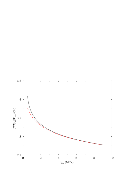
FIG. 4.: The exact one-loop radiative correction ${(\alpha/\pi)}g(E_{obs})$ in % (solid line) for reactions in Eq.(2) and the same correction in the limit $m_{e}\to 0$ (dashed line).

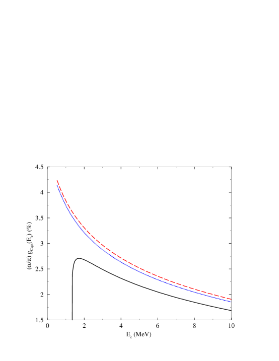
FIG. 5.: The electron energy dependence of the one-loop radiative corrections to the electron capture reactions in Eq. (84): $p+e^{-}\to n+\nu_{e}$ (solid line), $p+p+e^{-}\to d+\nu_{e}$ (dashed line), and ${}^{7}Be+e^{-}\to^{7}Li+\nu_{e}$ (dotted line).