Axial currents in electro-weak pion production
at threshold and in the $\Delta$-region

Abstract

We discuss electro-magnetic and weak production of pions on nucleons and show how results of experiments and their interpretation in terms of chiral quark models with explicit meson degrees of freedom combine to reveal the ground-state axial form factors and axial N-$\Delta$ transition amplitudes.

1 Introduction

The study of electro-weak N-$\Delta$ transition amplitudes, together with an understanding of the corresponding pion electro-production process at low energies, provides information on the structure of the nucleon and its first excited state. For example, the electro-magnetic transition amplitudes for the processes $\gamma^{\star}\mathrm{p}\to\Delta^{+}\to\mathrm{p}\pi^{0}$ and $\gamma^{\star}\mathrm{p}\to\Delta^{+}\to\mathrm{n}\pi^{+}$ are sensitive to the deviation of the nucleon shape from spherical symmetry aron . Below the $\Delta$ resonance (and in particular close to the pion-production threshold), the reaction $\gamma^{\star}\mathrm{p}\to\mathrm{n}\pi^{+}$ also yields information on the nucleon axial and induced pseudo-scalar form-factors. While the electro-production of pions at relatively high eprod_hiq and low eprod_loq ; arnd momentum transfers has been intensively investigated experimentally in the past years at modern electron accelerator facilities, very little data exist on the corresponding weak axial processes.

2 Nucleon axial form-factor

In a phenomenological approach, the nucleon axial form-factor is one of the quantities needed to extract the weak axial amplitudes in the $\Delta$ region. There are basically two methods to determine this form-factor. One set of experimental data comes from measurements of quasi-elastic (anti)neutrino scattering on protons, deuterons, heavier nuclei, and composite targets (see arnd for a comprehensive list of references). In the quasi-elastic picture of (anti)neutrino-nucleus scattering, the $\nu\mathrm{N}\to\mu\mathrm{N}$ weak transition amplitude can be expressed in terms of the nucleon electro-magnetic form-factors and the axial form factor $G_{\mathrm{A}}$. The axial form-factor is extracted by fitting the $Q^{2}$-dependence of the (anti)neutrino-nucleon cross section,

$${{\mathrm{d}}\sigma\over{\mathrm{d}}Q^{2}}=A(Q^{2})\mp B(Q^{2})\,(s-u)+C(Q^{2})\,(s-u)^{2}\>{,}$$ (1)

in which $G_{\mathrm{A}}(Q^{2})$ is contained in the $A(Q^{2})$, $B(Q^{2})$, and $C(Q^{2})$ coefficients and is assumed to be the only unknown quantity. It can be parameterised in terms of an ‘axial mass’ $M_{\mathrm{A}}$ as

$${G_{\mathrm{A}}(Q^{2})=G_{\mathrm{A}}(0)}/(1+Q^{2}/M_{\mathrm{A}}^{2})^{2}\>{.}$$

Another body of data comes from charged pion electro-production on protons (see arnd and references therein) slightly above the pion production threshold. As opposed to neutrino scattering, which is described by the Cabibbo-mixed $V-A$ theory, the extraction of the axial form factor from electro-production requires a more involved theoretical picture BKM1 ; axial_review . The presently available most precise determination for $M_{\mathrm{A}}$ from pion electro-production is

$$M_{\mathrm{A}}=(1.077\pm 0.039)\,\mathrm{GeV}$$ (2)

which is $\Delta M_{\mathrm{A}}=(0.051\pm 0.044)\,\mathrm{GeV}$ larger than the axial mass $M_{\mathrm{A}}=(1.026\pm 0.021)\,\mathrm{GeV}$ known from neutrino scattering experiments. The weighted world-average estimate from electro-production data is $M_{\mathrm{A}}=(1.069\pm 0.016)\,\mathrm{GeV}$, with an excess of $\Delta M_{\mathrm{A}}=(0.043\pm 0.026)\,\mathrm{GeV}$ with respect to the weak probe. The $\sim 5\,\%$ difference in $M_{\mathrm{A}}$ can apparently be attributed to pion-loop corrections to the electro-production process BKM1 .

3 N-$\Delta$ weak axial amplitudes

The experiments using neutrino scattering on deuterium or hydrogen in the $\Delta$ region have been performed at Argonne, CERN, and Brookhaven barish79 ; allen80 ; radecky82 ; kitagaki86 ; kitagaki90 . (Additional experimental results exist in the quasi-elastic regime, from which $M_{\mathrm{A}}$ has been extracted.) For pure $\Delta$ production, the matrix element has the familiar form

$$M=\langle\mu\Delta\,|\,\nu\mathrm{N}\rangle={G_{\mathrm{F}}\cos\theta_{\mathrm{C}}\over\sqrt{2}}\,j_{\alpha}\,\langle\Delta\,|\,V^{\alpha}-A^{\alpha}\,|\,\mathrm{N}\rangle\>{,}$$

where $G_{\mathrm{F}}$ is the Fermi’s coupling constant, $\theta_{\mathrm{C}}$ is the $V_{\mathrm{ud}}$ element of the CKM matrix, $j_{\alpha}=\overline{u}_{\mu}\gamma_{\alpha}(1-\gamma_{5})u_{\nu}$ is the matrix element of the leptonic current, and the matrix element of the hadronic current $J^{\alpha}$ has been split into its vector and axial parts. Typically either the $\Delta^{++}$ or the $\Delta^{+}$ are excited in the process. The hadronic part for the latter can be expanded in terms of weak vector and axial form-factors llewellyn72

$$M={G\over\sqrt{2}}\,\overline{u}_{\Delta\alpha}(p^{\prime})\,\biggl{\{} \left[\,{C_{3}^{\mathrm{V}}\over M}\,\gamma_{\mu}+{C_{4}^{\mathrm{V}}\over M^{2}}\,p_{\mu}^{\prime}+{C_{5}^{\mathrm{V}}\over M^{2}}\,p_{\mu}\,\right]\,\gamma_{5}F^{\mu\alpha}+{C_{6}^{\mathrm{V}}}\,j_{\alpha}\gamma_{5}$$

$$+ \left[\,{C_{3}^{\mathrm{A}}\over M}\,\gamma_{\mu}+{C_{4}^{\mathrm{A}}\over M^{2}}\,p_{\mu}^{\prime}\,\right]\,F^{\mu\alpha}+{C_{5}^{\mathrm{A}}}\,j^{\alpha}+{C_{6}^{\mathrm{A}}\over M^{2}}\,q^{\alpha}q^{\mu}j_{\mu}\,\biggr{\}}\,u(p)f(W)\>{,}$$

where $F^{\mu\alpha}=q^{\mu}j^{\alpha}-q^{\alpha}j^{\mu}$, $\overline{u}_{\Delta\alpha}(p^{\prime})$ is the Rarita-Schwinger spinor describing the $\Delta$ state with four-vector $p^{\prime}$, and $u(p)$ is the Dirac spinor for the (target) nucleon of mass $M$ with four-vector $p$. (In the case of the $\Delta^{++}$ excitation, the expression on the RHS acquires an additional isospin factor of $\sqrt{3}$ since $\langle\Delta^{++}\,|\,J^{\alpha}\,|\,\mathrm{p}\rangle=\sqrt{3}\langle\Delta^{+}\,|\,J^{\alpha}\,|\,\mathrm{p}\rangle=\sqrt{3}\langle\Delta^{0}\,|\,J^{\alpha}\,|\,\mathrm{p}\rangle$.) The function $f(W)$ represents a Breit-Wigner dependence on the invariant mass $W$ of the $\mathrm{N}\pi$ system.

The matrix element is assumed to be invariant under time reversal, hence all form-factors $C_{i}^{\mathrm{V,A}}(Q^{2})$ are real. Usually the conserved vector current hypothesis (CVC) is also assumed to hold. The CVC connects the matrix elements of the strangeness-conserving hadronic weak vector current to the isovector component of the electro-magnetic current:

$$\langle\Delta^{++}\,|\,V^{\alpha}\,|\,\mathrm{p}\rangle = \sqrt{3}\,\langle\Delta^{+}\,|\,J^{\alpha}_{\mathrm{EM}}(T=1)\,|\,\mathrm{p}\rangle\>{,}$$

$$\langle\Delta^{0}\,|\,V^{\alpha}\,|\,\mathrm{p}\rangle = \phantom{\sqrt{3}\,}\langle\Delta^{+}\,|\,J^{\alpha}_{\mathrm{EM}}(T=1)\,|\,\mathrm{p}\rangle\>{.}$$

The information on the weak vector transition form-factors $C_{i}^{\mathrm{V}}$ is obtained from the analysis of photo- and electro-production multipole amplitudes. For $\Delta$ electro-excitation, the allowed multipoles are the dominant magnetic dipole $M_{1+}$ and the electric and coulomb quadrupole amplitudes $E_{1+}$ and $S_{1+}$, which are found to be much smaller than $M_{1+}$ eprod_hiq ; eprod_loq . If we assume that $M_{1+}$ dominates the electro-production amplitude, we have $C_{5}^{\mathrm{V}}=C_{6}^{\mathrm{V}}=0$ and end up with only one independent vector form-factor

$$C_{4}^{\mathrm{V}}=-{M\over W}\,C_{3}^{\mathrm{V}}\>{.}$$

It turns out that electro-production data can be fitted well with a dipole form for $C_{3}^{\mathrm{V}}$,

$$C_{3}^{\mathrm{V}}(Q^{2})=2.05\,\biggl{[}\,1+{Q^{2}\over 0.54\,\mathrm{GeV}^{2}}\,\biggr{]}^{-2}\>{.}$$

An alternative parameterisation of $C_{3}^{\mathrm{V}}$ which accounts for a small observed deviation from the pure dipole form is

$$C_{3}^{\mathrm{V}}(Q^{2})=2.05\,\Bigl{[}\,1+9\sqrt{Q^{2}}\,\Bigr{]}\,\exp\Bigl{[}\,-6.3\sqrt{Q^{2}}\,\Bigr{]}\>{.}$$

The main interest therefore lies in the axial part of the hadronic weak current which is not well known.

Extraction of $C_{i}^{\mathrm{A}}(Q^{2})$ from data

The key assumption in experimental analyses of the axial matrix element is the PCAC. It implies that the divergence of the axial current should vanish as $m_{\pi}^{2}\to 0$, which occurs if the induced pseudo-scalar term with $C_{6}^{\mathrm{A}}$ (the analogue of $G_{\mathrm{P}}$ in the nucleon case) is dominated by the pion pole. In consequence, $C_{6}^{\mathrm{A}}$ can be expressed in terms of the strong $\pi\mathrm{N}\Delta$ form-factor,

$${C_{6}^{\mathrm{A}}(Q^{2})\over M^{2}}=f_{\pi}\sqrt{2\over 3}\,{G_{\pi\mathrm{N}\Delta}\over 2M}\,{1\over Q^{2}+m_{\pi}^{2}}\>{,}$$

while $C_{5}^{\mathrm{A}}$ and $C_{6}^{\mathrm{A}}$ can be approximately connected through the off-diagonal Goldberger-Treiman relation miniBled . In a phenomenological analysis, $C_{3}^{\mathrm{A}}(Q^{2})$, $C_{4}^{\mathrm{A}}(Q^{2})$, and $C_{5}^{\mathrm{A}}(Q^{2})$ are taken as free parameters and are fitted to the data. The axial form-factors are also parameterised in “corrected” dipole forms

$$C_{i}^{\mathrm{A}}(Q^{2})=C_{i}^{\mathrm{A}}(0)\,\biggl{[}\,1+{a_{i}Q^{2}\over b_{i}+Q^{2}}\,\biggr{]}\,\biggl{[}\,1+{Q^{2}\over M_{\mathrm{A}}^{2}}\,\biggr{]}^{-2}\>{.}$$

In the simplest approach one takes $a_{i}=b_{i}=0$. Historically, the experimental data on weak pion production could be understood well enough in terms of a theory developed by Adler adler . For lack of a better choice, Adler’s values for $C_{i}^{\mathrm{A}}(0)$ have conventionally been adopted to fix the fit-parameters at $Q^{2}=0$, i. e.

$$C_{3}^{\mathrm{A}}(0) = 0\>{,}$$ (3)

$$C_{4}^{\mathrm{A}}(0) = -0.3\>{,}$$ (4)

$$C_{5}^{\mathrm{A}}(0) = 1.2\>{.}$$ (5)

In such a situation, one ends up with $M_{\mathrm{A}}$ as the only free fit-parameter.

Several observables are used to fit the $Q^{2}$-dependence of the form-factors. Most commonly used are the total cross-sections $\sigma(E_{\nu})$, and the angular distributions of the recoiling nucleon

$${\mathrm{d}\sigma\over\mathrm{d}\Omega}={\sigma\over\sqrt{4\pi}}\,\biggl{[}\,Y_{00}-{2\over\sqrt{5}}\Bigl{[}\,\tilde{\rho}_{33}-{1\over 2}\,\Bigr{]}\,Y_{20}+{4\over\sqrt{10}}\,\tilde{\rho}_{31}\,\mathrm{Re}Y_{21}-{4\over\sqrt{10}}\,\tilde{\rho}_{3-1}\,\mathrm{Re}Y_{22}\,\biggr{]}\>{,}$$

where $\tilde{\rho}_{mn}$ are the density matrix elements and $Y_{LM}$ are the spherical harmonics. Better than from the $\tilde{\rho}_{mn}$ coefficients, the $Q^{2}$ dependence of the matrix element can be determined from the differential cross-section $\mathrm{d}\sigma/\mathrm{d}Q^{2}$. In particular, since the dependence on $C_{3}^{\mathrm{A}}$ and $C_{4}^{\mathrm{A}}$ is anticipated to be weak at $Q^{2}\sim 0$, then

$${\mathrm{d}\sigma\over\mathrm{d}Q^{2}}(Q^{2}=0)\propto(\,C_{5}^{\mathrm{A}}(0)\,)^{2}\>{.}$$

The refinements of this crude approach are dictated by several observations. If the target is a nucleus (for example, the deuteron which is needed to access specific charge channels), nuclear effects need to be estimated. Another important correction arises due to the finite energy width of the $\Delta$. In addition, the non-zero mass of the scattered muon may play a role at low $Q^{2}$.

All these effects have been addressed carefully in valencia . The sensitivity of the differential cross-section to different nucleon-nucleon potentials was seen to be smaller than $10\,\%$ even at $Q^{2}<0.1\,\mathrm{GeV}^{2}$. In the range above that value, this allows one to interpret inelastic data on the deuteron as if they were data obtained on the free nucleon. The effect of non-zero muon mass is even less pronounced: it does not exceed $5\,\%$ in the region of $Q^{2}\sim 0.05\,\mathrm{GeV}^{2}$. The energy dependence of the width of the $\Delta$ resonance was observed to have a negligible effect on the cross-section. The final value based on the analysis of Argonne data radecky82 is

$$C_{5}^{\mathrm{A}}(0)=1.22\pm 0.06\>{.}$$ (6)

At present, this is the best estimate for $C_{5}^{\mathrm{A}}(0)$, although a number of phenomenological predictions also exist mukh98 . We adopt this value for the purpose of comparison to our calculations. There is also some scarce, but direct experimental evidence from a free fit to the data that $C_{3}^{\mathrm{A}}(0)$ is indeed small and $C_{4}^{\mathrm{A}}(0)$ is close to the Adler’s value of $-0.3$ (see Figure 1). We use $C_{4}^{\mathrm{A}}(0)=-0.3$ in our comparisons in the next section.

Figure 1: One- and three-standard deviation limits on $C_{3}^{\mathrm{A}}(0)$ and $C_{4}^{\mathrm{A}}(0)$ as extracted from measurements of $\nu_{\mu}\mathrm{p}\to\mu^{-}\Delta^{++}$. The square denotes the model predictions by Adler adler . (Figure adapted after barish79 .)

4 Interpretation of $C_{i}^{\mathrm{A}}(Q^{2})$ in the linear $\sigma$-model

The axial N-$\Delta$ transition amplitudes can be interpreted in an illustrative way in quark models involving chiral fields like the linear $\sigma$-model (LSM), which may reveal the importance of non-quark degrees of freedom in baryons. Due to difficulties in consistent incorporation of the pion field, the model predictions for these amplitudes are very scarce Mukh . The present work FB18 ; letter02 was partly also motivated by the experience gained in the successful phenomenological description of the quadrupole electro-excitation of the $\Delta$ within the LSM, in which the pion cloud was shown to play a major role FGS .

4.1 Two-radial mode approach

We have realised that by treating the nucleon and the $\Delta$ in the LSM in a simpler, one-radial mode ansatz, the off-diagonal Goldberger-Treiman relation can not be satisfied. For the calculation of the amplitudes in the LSM, we have therefore used the two-radial mode ansatz for the physical baryon states which allows for different pion clouds around the bare baryons. The physical baryons are obtained from the superposition of bare quark cores and coherent states of mesons by the Peierls-Yoccoz angular projection. For the nucleon we have the ansatz

$$|\mathrm{N}\rangle=\mathcal{N}_{\mathrm{N}}P^{\scriptscriptstyle{1\over 2}}\left[\Phi_{\mathrm{N}}|\mathrm{N}_{q}\rangle+\Phi_{\mathrm{N}\Delta}|\Delta_{q}\rangle\right]\>{,}$$ (7)

where $\mathcal{N}_{\mathrm{N}}$ is the normalisation factor. Here $\Phi_{\mathrm{N}}$ and $\Phi_{\mathrm{N}\Delta}$ stand for hedgehog coherent states describing the pion cloud around the bare nucleon and bare $\Delta$, respectively, and $P^{\scriptscriptstyle{1\over 2}}$ is the projection operator on the subspace with isospin and angular momentum ${\textstyle{1\over 2}}$. Only one profile for the $\sigma$ field is assumed. For the $\Delta$ we assume a slightly different ansatz to ensure the proper asymptotic behaviour. We take

$$|\Delta\rangle=\mathcal{N}_{\Delta}\left\{P^{\scriptscriptstyle{3\over 2}}\Phi_{\Delta}|\Delta_{q}\rangle+\int\mathrm{d}k\,\eta(k)[a_{mt}^{\dagger}(k)|\mathrm{N}\rangle]^{{\scriptscriptstyle{3\over 2}}{\scriptscriptstyle{3\over 2}}}\right\}\,,$$ (8)

where $\mathcal{N}_{\Delta}$ is the normalisation factor, $|\mathrm{N}\rangle$ is the ground state and $[\,\,\,]^{{\scriptscriptstyle{3\over 2}}{\scriptscriptstyle{3\over 2}}}$ denotes the pion-nucleon state with isospin ${\textstyle{3\over 2}}$ and spin ${\textstyle{3\over 2}}$. We have interpreted the localised model states as wave-packets with definite linear momentum, as elaborated in miniBled .

4.2 Calculation of helicity amplitudes

We use the kinematics and notation of miniBled . For the quark contribution to the two transverse ($\lambda=1$) and longitudinal ($\lambda=0$) helicity amplitudes we obtain

$$\tilde{A}^{\mathrm{(q)}}_{s_{\Delta}\lambda} = -\langle\Delta_{s_{\Delta}\,{\scriptscriptstyle{1\over 2}}}|\int\mathrm{d}\mbox{\boldmath$r$}\,e^{\mathrm{i}kz}\psi^{\dagger}\alpha_{\lambda}\gamma_{5}{\textstyle{1\over 2}}\tau_{0}\psi|\mathrm{N}_{s_{\Delta}-\lambda\,{\scriptscriptstyle{1\over 2}}}\rangle$$

$$\tilde{A}^{(q)}_{s_{\Delta}\lambda} = -{\textstyle{1\over 2}}\mathcal{N}_{\Delta}\int\mathrm{d}r\,r^{2}\biggl{\{}$$

$$\biggl{[}j_{0}(kr)\biggl{(}u_{\Delta}u_{\mathrm{N}}-{1\over 3}v_{\Delta}v_{\mathrm{N}}\biggr{)}+{2\over 3}\,(3\lambda^{2}-2)\,j_{2}(kr)v_{\Delta}v_{\mathrm{N}}\biggr{]}\langle\Delta_{b}||\sigma\,\tau||\mathrm{N}\rangle$$

$$- c_{\eta} \biggl{[}j_{0}(kr)\biggl{(}u_{\mathrm{N}}^{2}-{1\over 3}v_{\mathrm{N}}^{2}\biggr{)}+{2\over 3}\,(3\lambda^{2}-2)\,j_{2}(kr)v_{\mathrm{N}}^{2}\biggr{]}$$

$$\times\biggl{[}{4\over 9}\langle\mathrm{N}||\sigma\tau||\mathrm{N}\rangle+{1\over 36}\langle\mathrm{N}||\sigma\tau||\mathrm{N}(J={\textstyle{3\over 2}})\rangle\biggr{]}\biggr{\}}C^{{\textstyle{3\over 2}}s_{\Delta}}_{{\textstyle{1\over 2}}s_{\Delta}-\lambda 1\lambda}C^{{\textstyle{3\over 2}}{\textstyle{1\over 2}}}_{{\textstyle{1\over 2}}{\textstyle{1\over 2}}10}\>{.}$$

Here $u$ and $v$ are upper and lower components of Dirac spinors for the nucleon and the $\Delta$, while $c_{\eta}$ is a coefficient involving integrals of the function $\eta(k)$ appearing in (8). The reduced matrix elements of $\sigma$$\tau$ can be expressed in terms of analytic functions with intrinsic numbers of pions as arguments. In all three cases, we take $s_{\Delta}={\textstyle{3\over 2}}$. For the scalar amplitudes, we take $\lambda=0$ and $s_{\Delta}={\textstyle{1\over 2}}$, and obtain

$$\tilde{S}^{\mathrm{(q)}} = -\langle\Delta_{{\scriptscriptstyle{1\over 2}}{\scriptscriptstyle{1\over 2}}}|\int\mathrm{d}\mbox{\boldmath$r$}\,e^{\mathrm{i}kz}\psi^{\dagger}\gamma_{5}{\textstyle{1\over 2}}\tau_{0}\psi|\mathrm{N}_{{\scriptscriptstyle{1\over 2}}{\scriptscriptstyle{1\over 2}}}\rangle$$

$$= {1\over 3}\,\mathcal{N}_{\Delta}\int\mathrm{d}r\,r^{2}\,j_{1}(kr)\left(u_{\Delta}v_{\mathrm{N}}-v_{\Delta}u_{\mathrm{N}}\right)\langle\Delta_{b}||\sigma\tau||\mathrm{N}\rangle\;.$$

For the non-pole meson contribution to the transverse and longitudinal helicity amplitudes we assume the same $\sigma$ profiles around the bare states, but different for the physical states. Introducing an “average” $\sigma$ field $\bar{\sigma}(r)\equiv{\textstyle{1\over 2}}(\sigma_{\mathrm{N}}(r)+\sigma_{\Delta}(r))$ we obtain

$$\tilde{A}^{\mathrm{(m)}}_{s_{\Delta}\lambda} = \langle\Delta_{s_{\Delta}\,{\scriptscriptstyle{1\over 2}}}|\int\mathrm{d}\mbox{\boldmath$r$}\,e^{\mathrm{i}kz}\left((\sigma-f_{\pi})\nabla_{\lambda}\pi_{0}-\pi_{0}\nabla_{\lambda}\sigma\right)|\mathrm{N}_{s_{\Delta}-\lambda\,{\scriptscriptstyle{1\over 2}}}\rangle$$

$$= {4\pi\over 3}\Biggl{\{}\int\mathrm{d}r\,r^{2}\,j_{0}(kr)\Biggl{[}\Biggl{(}(\bar{\sigma}-f_{\pi})\left({\mathrm{d}\varphi_{\Delta\mathrm{N}}\over\mathrm{d}r}+{2\varphi_{\Delta\mathrm{N}}\over r}\right)-{\mathrm{d}\bar{\sigma}\over\mathrm{d}r}\,\varphi_{\Delta\mathrm{N}}\Biggr{)}\Biggr{]}\Biggr{.}$$

$$\Biggl{.}+(3\lambda^{2}-2)\int\mathrm{d}r\,r^{2}\,j_{2}(kr)\Biggl{[}\Biggl{(}(\bar{\sigma}-f_{\pi})\left({\mathrm{d}\varphi_{\Delta\mathrm{N}}\over\mathrm{d}r}-{\varphi_{\Delta\mathrm{N}}\over r}\right)-{\mathrm{d}\bar{\sigma}\over\mathrm{d}r}\,\varphi_{\Delta\mathrm{N}}\Biggr{)}\Biggr{]}\Biggr{\}}$$

$$\times C^{{\textstyle{3\over 2}}s_{\Delta}}_{{\textstyle{1\over 2}}s_{\Delta}-\lambda 1\lambda}C^{{\textstyle{3\over 2}}{\textstyle{1\over 2}}}_{{\textstyle{1\over 2}}{\textstyle{1\over 2}}10}\>{,}$$

where $\varphi_{\Delta\mathrm{N}}=\langle\Delta\,|\,\pi\,|\,\mathrm{N}\rangle$. To compute the scalar amplitude, we make use of the off-diagonal virial relation derived in miniBled and define

$$\sigma^{P}(r)=\int_{0}^{\infty}\mathrm{d}k\,k^{2}\sqrt{k^{2}+m_{\sigma}^{2}}\sqrt{2\over\pi}\,j_{0}(kr)\,\sigma(k)\>{.}$$

We obtain

$$\tilde{S}^{\mathrm{(m)}} = -\langle\Delta_{{\scriptscriptstyle{1\over 2}}{\scriptscriptstyle{1\over 2}}}|\int\mathrm{d}\mbox{\boldmath$r$}\,e^{\mathrm{i}kz}\left((\sigma-f_{\pi})P_{\pi 0}-P_{\sigma}\pi_{0}\right)|\mathrm{N}_{{\scriptscriptstyle{1\over 2}}{\scriptscriptstyle{1\over 2}}}\rangle$$

$$= -{8\pi\over 3}\int\mathrm{d}r\,r^{2}\,j_{1}(kr)\left\{{\textstyle{1\over 2}}\left(\sigma^{P}_{\mathrm{N}}(r)-\sigma^{P}_{\Delta}(r)\right)\varphi_{\Delta\mathrm{N}}(r)-\left(\bar{\sigma}(r)-f_{\pi}\right)\omega_{*}\varphi_{\Delta\mathrm{N}}(r)\right\}\>{.}$$

By using

$$\tilde{A}_{s_{\Delta}\lambda}=\left(A^{0}-(3\lambda^{2}-2)A^{2}\right)C^{{\textstyle{3\over 2}}s_{\Delta}}_{{\textstyle{1\over 2}}s_{\Delta}-\lambda 1\lambda}C^{{\textstyle{3\over 2}}{\textstyle{1\over 2}}}_{{\textstyle{1\over 2}}{\textstyle{1\over 2}}10}\>{,}$$

the quark and non-pole meson contributions to the transverse amplitudes can finally be broken into $L=0$ and $L=2$ pieces,

$$\tilde{A}^{\mathrm{A}}_{\scriptscriptstyle{3\over 2}} = \sqrt{2\over 3}\left(A^{0}-A^{2}\right)\>{,}$$ (9)

$$\tilde{A}^{\mathrm{A}}_{\scriptscriptstyle{1\over 2}} = {1\over\sqrt{3}}\tilde{A}^{\mathrm{A}}_{\scriptscriptstyle{3\over 2}}={\sqrt{2}\over 3}\left(A^{0}-A^{2}\right)\>{,}$$ (10)

$$\tilde{L}^{\mathrm{A}} = {2\over 3}\left(A^{0}+2A^{2}\right)\>{,}$$ (11)

and inserted into (76), (77), and (78) of miniBled . The pole part of the meson contribution is

$$C^{\mathrm{A}}_{6\,\mathrm{(pole)}}(Q^{2})=f_{\pi}{G_{\pi\mathrm{N}\Delta}(Q^{2})\over 2M_{\mathrm{N}}}\,{M_{\mathrm{N}}^{2}\over m_{\pi}^{2}+Q^{2}}\,\sqrt{{2\over 3}}\>{.}$$

The strong $\mathrm{N}\Delta$ form-factor $G_{\pi\mathrm{N}\Delta}$ can be computed through

$${G_{\pi\mathrm{N}\Delta}(Q^{2})\over 2M_{\mathrm{N}}}{M_{\Delta}+M_{\mathrm{N}}\over 2M_{\Delta}}={1\over\mathrm{i}\,k}\,\langle\Delta\parallel\,\int\mathrm{d}\mbox{\boldmath$r$}\,\mathrm{e}^{\mathrm{i}\mbox{{\scriptsize\boldmath$k$}}\mbox{{\scriptsize\boldmath$r$}}}\,J(\mbox{\boldmath$r$})\,\parallel\mathrm{N}\rangle\>{,}$$

where the current $J$ has a component corresponding to the quark source and a component originating in the meson self-interaction term (see (58) of miniBled ),

$$J_{0}(\mbox{\boldmath$r$})=j_{0}(\mbox{\boldmath$r$})+{\partial U(\sigma,\vec{\pi})\over\partial\pi_{0}(\mbox{\boldmath$r$})}\>{.}$$

4.3 Results

Fig. 2 shows the $C^{\mathrm{A}}_{5}(Q^{2})$ amplitude with the quark-meson coupling constant of $g=4.3$ and $m_{\sigma}=600\,\mathrm{MeV}$ compared to the experimentally determined form-factors. The figure also shows the $C^{\mathrm{A}}_{5}(Q^{2})$ calculated from the strong $\pi\mathrm{N}\Delta$ form-factor using the off-diagonal Goldberger-Treiman relation.

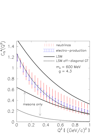
Figure 2: The amplitude $C_{5}^{\mathrm{A}}(Q^{2})$ in the two-radial mode LSM. The experimental uncertainty at $Q^{2}=0$ is given by Eq. (6). The error ranges are given by the spread in the axial-mass parameter $M_{\mathrm{A}}$ as determined from neutrino scattering experiments (broader range, kitagaki90 ) and from electro-production of pions (narrower range, Eq. (2)). Full curves: calculation from helicity amplitudes (9), (10), and (11); dashed curves: calculation from $G_{\pi\mathrm{N}\Delta}$.

The magnitude of $C_{5}^{\mathrm{A}}(Q^{2})$ is overestimated in the LSM, with $C_{5}^{\mathrm{A}}(0)$ about $25\,\%$ higher than the experimental average. Still, the $Q^{2}$-dependence follows the experimental one very well: the $M_{\mathrm{A}}$ from a dipole fit to our calculated values agrees to within a few percent with the experimental $M_{\mathrm{A}}$. On the other hand, with $C^{\mathrm{A}}_{5}(Q^{2})$ determined from the calculated strong $\pi\mathrm{N}\Delta$ form-factor, the absolute normalisation improves, while the $Q^{2}$ fall-off is steeper, with $M_{\mathrm{A}}\approx 0.80\,\mathrm{GeV}$. Since the model states are not exact eigenstates of the LSM Hamiltonian, the discrepancy between the two calculated values in some sense indicates the quality of the computational scheme. At $Q^{2}=-m_{\pi}^{2}$ where the off-diagonal Goldberger-Treiman relation is expected to hold, the discrepancy is $17\,\%$. The disagreement between the two approaches can be attributed to an over-estimate of the meson strength, a characteristic feature of LSM where only the meson fields bind the quarks.

Essentially the same trend is observed in the “diagonal” case: for the nucleon we obtain $g_{\mathrm{A}}=1.41$. The discrepancy with respect to the experimental value of $1.27$ is commensurate with the disagreement in $C_{5}^{\mathrm{A}}(0)$. The overestimate of $g_{\mathrm{A}}$ and $G_{\mathrm{A}}(Q^{2})$ was shown to persist even if the spurious centre-of-mass motion of the nucleon is removed fizika383 . An additional projection onto non-zero linear momentum therefore does not appear to be feasible.

The effect of the meson self-interaction is relatively less pronounced in the strong coupling constant (only $\sim 20\,\%$) than in $C^{\mathrm{A}}_{5}(Q^{2})$. Both $G_{\pi\mathrm{N}\Delta}(0)$ and $G_{\pi\mathrm{NN}}(0)$ are over-estimated in the model by $\sim 10\,\%$. Still, the ratio $G_{\pi\mathrm{N}\Delta}(0)/G_{\pi\mathrm{NN}}(0)=2.01$ is considerably higher than either the familiar SU(6) prediction $\sqrt{72/25}$ or the mass-corrected value of $1.65$ Hemmert , and compares reasonably well with the experimental value of $2.2$. This improvement is mostly a consequence of the renormalisation of the strong vertices due to pions.

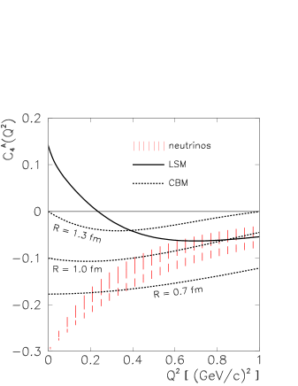
Figure 3: The amplitude $C_{4}^{\mathrm{A}}(Q^{2})$ in the two-radial mode linear $\sigma$-model, with model parameters and experimental uncertainties due to the spread in $M_{\mathrm{A}}$ as in Fig. 2, and in the Cloudy-Bag Model (see below for discussion). Experimentally, $C^{\mathrm{A}}_{4}(0)=-0.3\pm 0.5$ (see barish79 and Fig. 1). For orientation, the value for $C_{4}^{\mathrm{A}}(0)$ is used without error-bars.

The determination of the $C^{\mathrm{A}}_{4}(Q^{2})$ is less reliable because the meson contribution to the scalar component of this amplitude miniBled is very sensitive to small variations of the profiles. However, the experimental value is very uncertain as well. Neglecting the non-pole contribution to the scalar amplitude and $C_{6}^{\mathrm{A}}(Q^{2})$ (with the pole contribution canceling out), $C_{4}^{\mathrm{A}}(Q^{2})$ is fixed to $-(M_{\mathrm{N}}^{2}/2M_{\Delta}^{2})\,C_{5}^{\mathrm{A}}(Q^{2})$. At $Q^{2}=0$, this is in excellent numerical agreement with (4). In the LSM, the non-pole contribution to $C_{6}^{\mathrm{A}}(Q^{2})$ happens to be non-negligible and tends to increase $C_{4}^{\mathrm{A}}(Q^{2})$ at small $Q^{2}$, as seen in Fig. 3. An almost identical conclusion regarding $C^{\mathrm{A}}_{4}(Q^{2})$ applies in the case of the Cloudy-Bag Model, as shown below.

The $C^{\mathrm{A}}_{6}$ amplitude is governed by the pion pole for small values of $Q^{2}$ and hence by the value of $G_{\pi\mathrm{N}\Delta}$ which is well reproduced in the LSM, and underestimated by $\sim 35\,\%$ in the Cloudy-Bag Model. Fig. 4 shows that the non-pole contribution becomes relatively more important at larger values of $Q^{2}$.

Figure 4: The non-pole part and the total amplitude $C_{6}^{\mathrm{A}}(Q^{2})$ in the two-radial mode linear $\sigma$-model. Model parameters are as in Fig. 2.

5 Interpretation of $C_{i}^{\mathrm{A}}(Q^{2})$ in the Cloudy-Bag Model

For the calculation in the Cloudy-Bag Model (CBM) we have assumed the usual perturbative form for the pion profiles using the experimental masses for the nucleon and $\Delta$. Since the pion contribution to the axial current in the CBM has the form $f_{\pi}\partial^{\alpha}\mbox{\boldmath$\pi$}$, only the quarks contribute to the $C^{\mathrm{A}}_{4}(Q^{2})$ and $C^{\mathrm{A}}_{5}(Q^{2})$, while $C^{\mathrm{A}}_{6}(Q^{2})$ is almost completely dominated by the pion pole (see contribution by B. Golli miniBled ). With respect to the LSM, the sensitivity of the axial form-factors to the non-quark degrees of freedom is therefore almost reversed.

In the CBM, only the non-pole component of the axial current contributes to the amplitudes, and as a result the $C^{\mathrm{A}}_{5}(0)$ amplitude is less than $2/3$ of the experimental value. The behaviour of $C^{\mathrm{A}}_{5}(Q^{2})$ (see Fig. 5) is similar as in the pure MIT Bag Model (to within $10\,\%$), with fitted $M_{\mathrm{A}}\sim 1.2\,\mathrm{GeV\,fm}/R$. The off-diagonal Goldberger-Treiman relation is satisfied in the CBM, but $C^{\mathrm{A}}_{5}$ from $G_{\pi\mathrm{N}\Delta}$ has a steeper fall-off with fitted $M_{\mathrm{A}}\sim 0.8\,\mathrm{GeV\,fm}/R$.

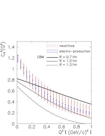
Figure 5: The amplitude $C_{5}^{\mathrm{A}}(Q^{2})$ in the Cloudy-Bag Model for three values of the bag radius. Experimental uncertainties are as in caption to Fig. 2.

The large discrepancy can be partly attributed to the fact that the CBM predicts a too low value for $G_{\pi\mathrm{NN}}$, and consequently $G_{\pi\mathrm{N}\Delta}$. We have found that the pions increase the $G_{\pi\mathrm{N}\Delta}/G_{\pi\mathrm{NN}}$ ratio by $\sim 15\,\%$ through vertex renormalisation. The effect is further enhanced by the mass-correction factor $2M_{\Delta}/(M_{\Delta}+M_{\mathrm{N}})$, yet suppressed in the kinematical extrapolation of $G_{\pi\mathrm{N}\Delta}(Q^{2})$ to the $\mathrm{SU}(6)$ limit. This suppression is weaker at small bag radii $R$: the ratio drops from $2.05$ at $R=0.7\,\mathrm{fm}$ to $1.60$ (below the $\mathrm{SU}(6)$ value) at $R=1.3\,\mathrm{fm}$.

The determination of the $C^{\mathrm{A}}_{4}(Q^{2})$ is less reliable for very much the same reason as in the LSM. The non-pole contribution to $C_{6}^{\mathrm{A}}(Q^{2})$ tends to add to the excessive strength of $C_{4}^{\mathrm{A}}(Q^{2})$ at low $Q^{2}$, as seen in Fig. 3. Never the less, the experimental data are too coarse to allow for a meaningful comparison to the model. For technical details regarding the calculation in the CBM, refer to miniBled .

References

• (1) A. M. Bernstein, to appear in Proceedings of the VII Conference on Electron-Nucleus Scattering, June 24-28, 2002, Elba, Italy.
• (2) K. Joo et al., Phys. Rev. Lett. 88 (2002) 122001;
J. Volmer et al., Phys. Rev. Lett. 86 (2001) 1713;
D. Gaskell et al., Phys. Rev. Lett. 87 (2001) 202301;
V. Frolov et al., Phys. Rev. Lett. 82 (1999) 45.
• (3) Th. Pospischil et al., Phys. Rev. Lett. 86 (2001) 2959;
C. Mertz et al., Phys. Rev. Lett. 86 (2001) 2963;
S. Choi et al., Phys. Rev. Lett. 71 (1993) 3927.
• (4) A. Liesenfeld et al., Phys. Lett. B 468 (1999) 20.
• (5) V. Bernard, N. Kaiser, U.–G. Meißner, Phys. Rev. Lett. 69 (1992) 1877;
V. Bernard, N. Kaiser and U.–G. Meißner, Phys. Rev. Lett. 72 (1994) 2810.
• (6) V. Bernard, L. Elouadrhiri, U.–G. Meißner, J. Phys. G: Nucl. Part. Phys. 28 (2002) R1.
• (7) S. J. Barish et al., Phys. Rev. D 19 (1979) 2521.
• (8) P. Allen et al., Nucl. Phys. B 176 (1980) 269.
• (9) G. M. Radecky et al., Phys. Rev. D 25 (1982) 1161.
• (10) T. Kitagaki et al., Phys. Rev. D 34 (1986) 2554.
• (11) T. Kitagaki et al., Phys. Rev. D 42 (1990) 1331.
• (12) C. H. Llewellyn Smith, Phys. Rep. 3C (1972) 261.
• (13) B. Golli, L. Amoreira, M. Fiolhais, S. Širca, these Proceedings; hep-ph/0211293
• (14) S. Adler, Ann. Phys. 50 (1968) 189.
• (15) S. K. Singh, M. J. Vicente-Vacas, E. Oset, Phys. Lett. B 416 (1998) 23;
L. Alvarez-Ruso, S. K. Singh, M. J. Vicente-Vacas, Phys. Rev. C 57 (1998) 2693;
L. Alvarez-Ruso, S. K. Singh, M. J. Vicente-Vacas, Phys. Rev. C 59 (1999) 3386;
L. Alvarez-Ruso, E. Oset, S. K. Singh, M. J. Vicente-Vacas, Nucl. Phys. A 663/664 (2000) 837c.
• (16) N. C. Mukhopadhyay et al., Nucl. Phys. A 633 (1998) 481.
• (17) Jùn Líu, N. C. Mukhopadhyay, L. Zhang, Phys. Rev. C 52 (1995) 1630.
• (18) S. Širca, L. Amoreira, M. Fiolhais, B. Golli, to appear in R. Krivec, B. Golli, M. Rosina, S. Širca (eds.), Proceedings of the XVIII European Conference on Few-Body Problems in Physics, 7–14 September 2002, Bled, Slovenia; hep-ph/0211290
• (19) B. Golli, S. Širca, L. Amoreira, and M. Fiolhais, submitted for publication in Phys. Lett. B, hep-ph/0210014.
• (20) M. Fiolhais, B. Golli, S. Širca, Phys. Lett. B 373 (1996) 229.
• (21) M. Rosina, M. Fiolhais, B. Golli, S. Širca, Proceedings of the “Nuclear and Particle Physics with CEBAF at Jefferson Lab” Meeting, November 3–10, 1998, Dubrovnik, Croatia, Fizika B 8 (1999) 383.
• (22) T. R. Hemmert, B. R. Holstein, N. C. Mukhopadhyay, Phys. Rev. D 51 (1995) 158.