HD-THEP-02-22
hep-ph/0211287
Confining QCD Strings, Casimir Scaling, and a Euclidean Approach to High-Energy Scattering

Abstract

We compute the chromo-field distributions of static color dipoles in the fundamental and adjoint representation of $SU(N_{c})$ in the loop-loop correlation model and find Casimir scaling in agreement with recent lattice results. Our model combines perturbative gluon exchange with the non-perturbative stochastic vacuum model which leads to confinement of the color charges in the dipole via a string of color fields. We compute the energy stored in the confining string and use low-energy theorems to show consistency with the static quark-antiquark potential. We generalize Meggiolaro’s analytic continuation from parton-parton to gauge-invariant dipole-dipole scattering and obtain a Euclidean approach to high-energy scattering that allows us in principle to calculate $S$-matrix elements directly in lattice simulations of QCD. We apply this approach and compute the $S$-matrix element for high-energy dipole-dipole scattering with the presented Euclidean loop-loop correlation model. The result confirms the analytic continuation of the gluon field strength correlator used in all earlier applications of the stochastic vacuum model to high-energy scattering.

Keywords: Casimir Scaling, Confining String, Flux Tube, High-Energy Scattering, Low-Energy Theorems, Static Potential, Stochastic Vacuum Model

PACS numbers: 12.38.-t, 12.38.Lg, 11.80.Fv

1 Introduction

The structure of the QCD vacuum is responsible for color confinement, spontaneous chiral symmetry breaking, and dynamical mass generation [1]. Hadronic reactions are expected to show further manifestations of a non-trivial QCD vacuum. It is indeed a key issue to unravel the effects of confinement and topologically non-trivial gauge field configurations (such as instantons) on such reactions [2, 3]. Moreover, it would be a significant breakthrough to understand the size, behavior and growth of hadronic cross sections with increasing c.m. energy from the QCD Lagrangian.

Lattice QCD is the principal theoretical tool to study the QCD vacuum from first principles. Numerical simulations of QCD on Euclidean lattices give strong evidence for color confinement and spontaneous chiral symmetry breaking and describe dynamical mass generation from the QCD Lagrangian [4, 5, 6]. However, since lattice QCD is limited to the Euclidean formulation of QCD, it cannot be applied in Minkowski space-time to simulate high-energy reactions in which particles are moving near the light cone. Furthermore, although lattice investigations have significantly enhanced our understanding of non-perturbative phenomena and particularly confinement, one can quote the concluding sentence of Greensite’s recent review [7]: “The confinement problem is still open, and remains a major intellectual challenge in our field.” Here (phenomenological) models that allow analytic calculations are important as they provide valuable complementary insights.

In this work we introduce the Euclidean version of the loop-loop correlation model (LLCM) which has been developed in Minkowski space-time to describe high-energy reactions of hadrons and photons [8] on the basis of a functional integral approach [9, 10, 11, 12, 13]. The central element in our approach is the gauge-invariant Wegner-Wilson loop [14, 15]: The physical quantities considered are obtained from the vacuum expectation value (VEV) of one Wegner-Wilson loop, $\langle W_{r}[C]\rangle$, and the correlation of two Wegner-Wilson loops, $\langle W_{r_{1}}[C_{1}]W_{r_{2}}[C_{2}]\rangle$. Here $r_{(i)}$ indicates the $SU(N_{c})$ representation of the Wegner-Wilson loops which we keep as general as possible. We express $\langle W_{r}[C]\rangle$ and $\langle W_{r_{1}}[C_{1}]W_{r_{2}}[C_{2}]\rangle$ in terms of the gauge-invariant bilocal gluon field strength correlator integrated over minimal surfaces by using the non-Abelian Stokes theorem [16] and a matrix cumulant expansion [17] in the Gaussian approximation. The latter approximation relies on the assumption of a Gaussian dominance in the correlations of gauge-invariant non-local gluon field strengths, i.e. the dominance of the bilocal correlator over higher ones, and is supported by lattice investigations [18]. In our model this Gaussian approximation leads directly to the Casimir scaling of the static quark-antiquark potential which for $SU(3)$ has clearly been confirmed on the lattice [19, 20]. We decompose the gauge-invariant bilocal gluon field strength correlator into a perturbative and a non-perturbative component: The stochastic vacuum model (SVM) [21] is used for the non-perturbative low-frequency background field and perturbative gluon exchange for the additional high-frequency contributions. This combination allows us to describe long and short distance correlations in agreement with lattice calculations of the gluon field strength correlator [22, 23, 18, 24]. Moreover, it leads to a static quark-antiquark potential with color Coulomb behavior for small and confining linear rise for large source separations. We calculate the static quark-antiquark potential with the LLCM parameters determined in fits to high-energy scattering data [8] and find good agreement with lattice data. We thus have one model that describes both static hadronic properties and high-energy reactions of hadrons and photons in good agreement with experimental and lattice QCD data.

We apply the LLCM to compute the chromo-electric fields generated by a static color dipole in the fundamental and adjoint representation of $SU(N_{c})$. The non-perturbative SVM component describes the formation of a color flux tube that confines the two color sources in the dipole [25] while the perturbative component leads to color Coulomb fields. We find Casimir scaling for both the perturbative and non-perturbative contributions to the chromo-electric fields again as a direct consequence of the Gaussian appoximation in the gluon field strengths. The mean squared radius of the confining QCD string is calculated as a function of the dipole size. Transverse and longitudinal energy density profiles are provided to study the interplay between perturbative and non-perturbative physics for different dipole sizes. The transition from perturbative to string behavior is found at source separations of about $0.5\,\mbox{fm}$ in agreement with the recent results of Lüscher and Weisz [26].

The low-energy theorems, known in lattice QCD as Michael sum rules [27], relate the energy and action stored in the chromo-fields of a static color dipole to the corresponding ground state energy. The Michael sum rules, however, are incomplete in their original form [27]. We present the complete energy and action sum rules [28, 29, 30] in continuum theory taking into account the contributions to the action sum rule found in [31] and the trace anomaly contribution to the energy sum rule [28]. Using these low-energy theorems, we compare the energy and action stored in the confining string with the confining part of the static quark-antiquark potential. This allows us to confirm consistency of the model results and to determine the values of the Callan-Symanzik $\beta$ function and the strong coupling $\alpha_{s}$ at the renormalization scale at which the non-perturbative SVM component is working. The values obtained for $\beta$ and $\alpha_{s}$ are compared to model independent QCD results for the Callan-Symanzik function. Earlier investigations along these lines have been incomplete since only the contribution from the traceless part of the energy-momentum tensor has been considered in the energy sum rule.

To study the effect of the confining QCD string examined in Euclidean space-time on high-energy reactions in Minkowski space-time, an analytic continuation from Euclidean to Minkowski space-time is needed. For investigations of high-energy reactions in our Euclidean model, the gauge-invariant bilocal gluon field strength correlator can be analytically continued from Euclidean to Minkowski space-time. This analytic continuation has been introduced for applications of the SVM to high-energy reactions [11, 12, 13] and is used in our Minkowskian applications of the LLCM [8, 32, 33, 34]. Recently, an alternative analytic continuation for parton-parton scattering has been established in the perturbative context by Meggiolaro [35]. This analytic continuation has already been used to access high-energy scattering from the supergravity side of the AdS/CFT correspondence [36], which requires a positive definite metric in the definition of the minimal surface [37], and to examine the effect of instantons on high-energy scattering [38].

In this work we generalize Meggiolaro’s analytic continuation [35] from parton-parton to gauge-invariant dipole-dipole scattering such that $S$-matrix elements for high-energy reactions can be computed from configurations of Wegner-Wilson loops in Euclidean space-time and with Euclidean functional integrals. This shows how one can access high-energy reactions directly in lattice QCD. First attempts in this direction have already been carried out but only very few signals could be extracted, while most of the data was dominated by noise [39]. We apply this approach to compute the scattering of dipoles at high-energy in the Euclidean LLCM. We recover exactly the result derived with the analytic continuation of the gluon field strength correlator [8]. This confirms the analytic continuation used in all earlier applications of the stochastic vacuum model to high-energy scattering [11, 12, 13, 40, 41, 42, 43, 44, 45, 48, 46, 47] including the Minkowskian applications of the LLCM [8, 32, 33, 34]. In fact, the $S$-matrix element obtained has already been used as the basis for a unified description of hadronic high-energy reactions [8], to study saturation effects in hadronic cross sections [8, 32, 34], and to investigate manifestations of the confining QCD string in high-energy reactions of photons and hadrons [33].

The outline of the paper is as follows. In Sec. 2 the LLCM is introduced in its Euclidean version and the general computations of $\langle W_{r}[C]\rangle$ and $\langle W_{r_{1}}[C_{1}]W_{r_{2}}[C_{2}]\rangle$ are presented. Based on these evaluations, we compute the potential of a static color dipole in Sec. 3 and the associated chromo-field distributions in Sec. 4 with emphasis on Casimir scaling and the interplay between perturbative color Coulomb behavior and non-perturbative formation of the confining QCD string. In Sec. 5 low-energy theorems are discussed and used to show consistency of the model results and to determine the values of $\beta$ and $\alpha_{s}$ at the renormalization scale at which the non-perturbative SVM component is working. In Sec. 6 the Euclidean approach to high-energy scattering is presented and applied to compute high-energy dipole-dipole scattering in our Euclidean model. In the Appendixes we review the derivation of the non-Abelian Stokes theorem, give parametrizations of the loops and the minimal surfaces, and provide the detailed computations for the results in the main text.

2 The Loop-Loop Correlation Model

In this section the vacuum expectation value of one Wegner-Wilson loop and the correlation of two Wegner-Wilson loops are computed for arbitrary loop geometries within a Gaussian approximation in the gluon field strengths. The results are applied in the following sections. We describe our model for the QCD vacuum in which the stochastic vacuum model [21] is used for the non-perturbative low-frequency background field (long-distance correlations) and perturbative gluon exchange for the additional high-frequency contributions (short-distance correlations).

2.1 Vacuum Expectation Value of one Wegner-Wilson Loop

A crucial quantity in gauge theories is the Wegner-Wilson loop operator [14, 15]

$$W_{r}[C]=\tilde{\mbox{Tr}}_{r}\,{\cal P}\exp\!\left[-ig\oint_{\scriptsize C}dZ_{\mu}\,{\cal G}_{\mu}^{a}(Z)\,t_{r}^{a}\right]\ .$$ (2.1)

Concentrating on $SU(N_{c})$ Wegner-Wilson loops, where $N_{c}$ is the number of colors, the subscript $r$ indicates a representation of $SU(N_{c})$, $\tilde{\mbox{Tr}}_{r}=\mbox{Tr}_{r}(\cdots)/\mbox{Tr}{1\!\rm l}_{r}$ is the normalized trace in the corresponding color space with unit element ${1\!\rm l}_{r}$, $g$ is the strong coupling, and ${\cal G}_{\mu}(Z)={\cal G}_{\mu}^{a}(Z)t_{r}^{a}$ represents the gluon field with the $SU(N_{c})$ group generators in the corresponding representation, $t_{r}^{a}$, that demand the path ordering indicated by ${\cal P}$ on the closed path $C$ in space-time. A distinguishing theoretical feature of the Wegner-Wilson loop is its invariance under local gauge transformations in color space. Therefore, it is the basic object in lattice gauge theories [14, 15, 4] and has been considered as the fundamental building block for a gauge theory in terms of gauge invariant variables [49]. Phenomenologically, the Wegner-Wilson loop represents the phase factor associated with the propagation of a very massive color source in the representation $r$ of the gauge group $SU(N_{c})$.

To compute the expectation value of the Wegner-Wilson loop (2.1) in the QCD vacuum

$$\Big{\langle}W_{r}[C]\Big{\rangle}_{G}=\Big{\langle}\tilde{\mbox{Tr}}_{r}\,{\cal P}\exp\!\left[-i\,g\oint_{\scriptsize C}dZ_{\mu}\,{\cal G}_{\mu}^{a}(Z)\,t_{r}^{a}\right]\Big{\rangle}_{G}\ ,$$ (2.2)

we transform the line integral over the loop $C$ into an integral over the surface $S$ with $\partial S=C$ by applying the non-Abelian Stokes theorem [16]

$$\Big{\langle}W_{r}[C]\Big{\rangle}_{G}=\Big{\langle}\tilde{\mbox{Tr}}_{r}\,{\cal P}_{S}\exp\left[-i\,\frac{g}{2}\int_{S}\!d\sigma_{\mu\nu}(Z){\cal G}^{a}_{\mu\nu}(O,Z;C_{ZO})\,t_{r}^{a}\right]\Big{\rangle}_{G}\ ,$$ (2.3)

where ${\cal P}_{S}$ indicates surface ordering and $O$ is an arbitrary reference point on the surface $S$. In Eq. (2.3) the gluon field strength tensor, ${\cal G}_{\mu\nu}(Z)={\cal G}_{\mu\nu}^{a}(Z)\,t_{r}^{a}$, is parallel transported to the reference point $O$ along the path $C_{ZO}$,

$${\cal G}_{\mu\nu}(O,Z;C_{ZO})=\Phi_{r}(O,Z;C_{ZO}){\cal G}_{\mu\nu}(Z)\Phi_{r}(O,Z;C_{ZO})^{-1}\ ,$$ (2.4)

with the QCD Schwinger string

$$\Phi_{r}(O,Z;C_{ZO})={\cal P}\exp\left[-i\,g\int_{C_{ZO}}\!\!dZ_{\mu}{\cal G}^{a}_{\mu}(Z)\,t_{r}^{a}\right]\ .$$ (2.5)

A more detailed explanation of the non-Abelian Stokes theorem and the associated surface ordering is given in Appendix A.

The QCD vacuum expectation value $\langle\ldots\rangle_{G}$ represents functional integrals in which the functional integration over the fermion fields has already been carried out as indicated by the subscript $G$ [10]. The model we use for the evaluation of $\langle\ldots\rangle_{G}$ is based on the quenched approximation which does not allow string breaking through dynamical quark-antiquark production. So far, it is not clear how to introduce dynamical quarks into this model. One suggestion is presented in Appendix A of Ref. [10].

Due to the linearity of the functional integral, $\langle\tilde{\mbox{Tr}}_{r}\ldots\rangle=\tilde{\mbox{Tr}}_{r}\langle\ldots\rangle$, we can write

$$\Big{\langle}W_{r}[C]\Big{\rangle}_{G}=\tilde{\mbox{Tr}}_{r}\Big{\langle}{\cal P}_{S}\exp\left[-i\,\frac{g}{2}\int_{S}\!d\sigma_{\mu\nu}(Z){\cal G}^{a}_{\mu\nu}(O,Z;C_{ZO})\,t_{r}^{a}\right]\Big{\rangle}_{G}\ .$$ (2.6)

For the evaluation of (2.6), a matrix cumulant expansion is used as explained in [10] (cf. also [17])

$$\Big{\langle}{\cal P}_{S}\,\exp\left[-i\,\frac{g}{2}\int_{S}\!d\sigma(Z){\cal G}(O,Z;C_{ZO})\right]\Big{\rangle}_{G}$$

$$=\exp[\,\,\sum_{n=1}^{\infty}\frac{1}{n!}(-i\,\frac{g}{2})^{n}\int d\sigma(X_{1})\cdots d\sigma(X_{n})\,K_{n}(X_{1},\cdots,X_{n})]\ ,$$ (2.7)

where space-time indices are suppressed to simplify notation. The cumulants $K_{n}$ consist of expectation values of ordered products of the non-commuting matrices ${\cal G}(O,Z;C_{ZO})$. The leading matrix cumulants are

$$K_{1}(X) = \langle{\cal G}(O,X;C_{X})\rangle_{G},$$ (2.8)

$$K_{2}(X_{1},X_{2}) = \langle{\cal P}_{S}[{\cal G}(O,X_{1};C_{X_{1}}){\cal G}(O,X_{2};C_{X_{2}})]\rangle_{G}$$ (2.9)

$$-\frac{1}{2}\left[\langle{\cal G}(O,X_{1};C_{X_{1}})\rangle_{G}\langle{\cal G}(O,X_{2};C_{X_{2}})\rangle_{G}+(1\leftrightarrow 2)\,\right]\ .$$

Since the vacuum does not prefer a specific color direction, $K_{1}$ vanishes and $K_{2}$ becomes

$$K_{2}(X_{1},X_{2})=\langle{\cal P}_{S}[{\cal G}(O,X_{1};C_{X_{1}}){\cal G}(O,X_{2};C_{X_{2}})]\rangle_{G}\ .$$ (2.10)

Now, we approximate the functional integral associated with the expectation values $\langle\ldots\rangle_{G}$ as a Gaussian integral in the parallel transported gluon field strength (2.4). This Gaussian approximation is supported by lattice investigations [18] that show a dominance of the bilocal gauge-invariant gluon field strength correlator over higher-point non-local correlators. As a consequence of the Gaussian approximation, the cumulants factorize into two-point field correlators such that all higher cumulants, $K_{n}$ with $n>2$, vanish. Thus, $\langle W_{r}[C]\rangle_{G}$ can be expressed in terms of $K_{2}$

$$\!\!\!\!\!\!\!\!\!\!\!\Big{\langle}W_{r}[C]\Big{\rangle}_{G}=\tilde{\mbox{Tr}}_{r}\exp\!\left[-\frac{g^{2}}{8}\!\int_{S}\!d\sigma_{\mu\nu}(X_{1})\!\int_{S}\!d\sigma_{\rho\sigma}(X_{2})\right.$$

$$\!\!\!\!\!\!\!\!\!\!\!\hphantom{\Big{\langle}W_{r}[C]\Big{\rangle}_{G}=\tilde{\mbox{Tr}}_{r}\exp}\left.\Big{\langle}{\cal P}_{S}[{\cal G}^{a}_{\mu\nu}(O,X_{1};C_{X_{1}O})\,t_{r}^{a}\,\,{\cal G}^{b}_{\rho\sigma}(O,X_{2};C_{X_{2}O})\,t_{r}^{b}]\Big{\rangle}_{G}\right]$$ (2.11)

Due to the color neutrality of the vacuum, the gauge-invariant bilocal gluon field strength correlator contains a $\delta$ function in color space,

$$\Big{\langle}\frac{g^{2}}{4\pi^{2}}\left[{\cal G}^{a}_{\mu\nu}(O,X_{1};C_{X_{1}O}){\cal G}^{b}_{\rho\sigma}(O,X_{2};C_{X_{2}O})\right]\Big{\rangle}_{G}=:\frac{1}{4}\delta^{ab}F_{\mu\nu\rho\sigma}(X_{1},X_{2},O;C_{X_{1}O},C_{X_{2}O})$$ (2.12)

which makes the surface ordering ${\cal P}_{S}$ in (2.11) irrelevant. The tensor $F_{\mu\nu\rho\sigma}$ will be specified in Sec. 2.3. With (2.12) and the quadratic Casimir operator $C_{2}(r)$,

$$t_{r}^{a}\,t_{r}^{a}=t_{r}^{2}=C_{2}(r)\,{1\!\rm l}_{r}\ ,$$ (2.13)

Eq. (2.11) reads

$$\Big{\langle}W_{r}[C]\Big{\rangle}_{G}=\tilde{\mbox{Tr}}_{r}\exp\left[-\frac{C_{2}(r)}{2}\,\chi_{SS}\,{1\!\rm l}_{r}\right]=\exp\left[-\frac{C_{2}(r)}{2}\,\chi_{SS}\right]\ ,$$ (2.14)

where

$$\chi_{SS}:=\frac{\pi^{2}}{4}\int_{S}\!d\sigma_{\mu\nu}(X_{1})\int_{S}\!d\sigma_{\rho\sigma}(X_{2})F_{\mu\nu\rho\sigma}(X_{1},X_{2},O;C_{X_{1}O},C_{X_{2}O})\ .$$ (2.15)

In this rather general result (2.14) obtained directly from the color neutrality of the QCD vacuum and the Gaussian approximation in the gluon field strengths, the more detailed aspects of the QCD vacuum and the geometry of the considered Wegner-Wilson loop are encoded in the function $\chi_{SS}$ which is computed in Appendix C for a rectangular loop.

In explicit computations we use for $S$ the minimal surface, which is the planar surface spanned by the loop ($C=\partial S$) that leads most naturally to Wilson’s area law [21]. Of course, the results should not depend on the choice of the surface. In our model the perturbative and non-perturbative non-confining components satisfy this requirement. The non-perturbative confining component in $F_{\mu\nu\rho\sigma}$ depends on the choice of the surface due to the Gaussian approximation and the associated truncation of the cumulant expansion. Since the minimal surface leads to a static quark-antiquark potential that is in good agreement with lattice data (see Sec. 3), we think that the minimal surface reduces the contribution from higher cumulants. Within bosonic string theory, our minimal surface represents the world-sheet of a rigid string: Our model does not describe fluctuations or excitations of the string and thus cannot reproduce the Lüscher term which has recently been confirmed by Lüscher and Weisz [26].

2.2 The Loop-Loop Correlation Function

The computation of the loop-loop correlation function $\langle W_{r_{1}}[C_{1}]W_{r_{2}}[C_{2}]\rangle_{G}$ starts again with the application of the non-Abelian Stokes theorem [16] which allows us to transform the line integrals over the loops $C_{1,2}$ into integrals over surfaces $S_{1,2}$ with $\partial S_{1,2}=C_{1,2}$

$$\Big{\langle}W_{r_{1}}[C_{1}]W_{r_{2}}[C_{2}]\Big{\rangle}_{G}=\Big{\langle}\tilde{\mbox{Tr}}_{r_{1}}\,{\cal P}_{S}\exp\left[-i\,\frac{g}{2}\int_{S_{1}}\!d\sigma_{\mu\nu}(X_{1}){\cal G}^{a}_{\mu\nu}(O_{1},X_{1};C_{X_{1}O_{1}})\,t_{r_{1}}^{a}\right]$$

$$\quad\quad\quad\quad\quad\times\,\tilde{\mbox{Tr}}_{r_{2}}\,{\cal P}_{S}\exp\left[-i\,\frac{g}{2}\int_{S_{2}}\!d\sigma_{\rho\sigma}(X_{2}){\cal G}^{b}_{\rho\sigma}(O_{2},X_{2};C_{X_{2}O_{2}})\,t_{r_{2}}^{b}\right]\Big{\rangle}_{G}$$ (2.16)

where $O_{1}$ and $O_{2}$ are the reference points on the surfaces $S_{1}$ and $S_{2}$, respectively, that enter through the non-Abelian Stokes theorem. In order to ensure gauge invariance in our model, the gluon field strengths associated with the loops must be compared at one reference point $O$. Due to this physical constraint, the surfaces $S_{1}$ and $S_{2}$ are required to touch at a common reference point $O_{1}=O_{2}=O$.

To treat the product of the two traces in (2.16), we transfer the approach of Berger and Nachtmann [45] (cf. also [8]) to Euclidean space-time. Accordingly, the product of the two traces, $\tilde{\mbox{Tr}}_{r_{1}}(\cdots)\,\tilde{\mbox{Tr}}_{r_{2}}(\cdots)$, over $SU(N_{c})$ matrices in the $r_{1}$ and $r_{2}$ representations, respectively, is interpreted as one trace $\tilde{\mbox{Tr}}_{r_{1}\otimes r_{2}}(\cdots):=\mbox{Tr}_{r_{1}\otimes r_{2}}(\cdots)/\mbox{Tr}_{r_{1}\otimes r_{2}}({1\!\rm l}_{r_{1}\otimes r_{2}})$ that acts in the tensor product space built from the $r_{1}$ and $r_{2}$ representations,

$$\Big{\langle}W_{\!r_{1}}[C_{1}]W_{\!r_{2}}[C_{2}]\Big{\rangle}_{G}\!\!\!\! \!\!\!=\!\!\! \!\Big{\langle}\tilde{\mbox{Tr}}_{r_{1}\otimes r_{2}}\!\left\{\!\!\Big{[}{\cal P}_{S}\exp\!\big{[}\!-\!i\frac{g}{2}\!\int_{S_{1}}\!\!\!\!d\sigma_{\mu\nu}(X_{1}){\cal G}^{a}_{\mu\nu}(O,X_{1};C_{X_{1}O})\,t_{r_{1}}^{a}\big{]}\,\otimes\,{1\!\rm l}_{r_{2}}\Big{]}\right.$$ (2.17)

$$\!\!\!\!\!\!\!\!\!\!\!\!\!\times\left.\Big{[}{1\!\rm l}_{r_{1}}\,\otimes\,{\cal P}_{S}\exp\!\big{[}\!-\!i\frac{g}{2}\!\int_{S_{2}}\!\!\!\!d\sigma_{\rho\sigma}(X_{2}){\cal G}^{b}_{\rho\sigma}(O,X_{2};C_{X_{2}O})\,t_{r_{2}}^{b}\big{]}\Big{]}\!\!\right\}\!\Big{\rangle}_{G}$$

With the identities

$$\exp\left(\,t_{r_{1}}^{a}\,\right)\,\otimes\,{1\!\rm l}_{r_{2}} = \exp\left(\,t_{r_{1}}^{a}\,\otimes\,{1\!\rm l}_{r_{2}}\,\right)\ ,$$ (2.18)

$${1\!\rm l}_{r_{1}}\,\otimes\,\exp\left(\,t_{r_{2}}^{a}\,\right) = \exp\left(\,{1\!\rm l}_{r_{1}}\,\otimes\,t_{r_{2}}^{a}\,\right)\ ,$$ (2.19)

the tensor products can be shifted into the exponents. Using the matrix multiplication relations in the tensor product space

$$\big{(}t_{r_{1}}^{a}\,\otimes\,{1\!\rm l}_{r_{2}}\big{)}\big{(}t_{r_{1}}^{b}\,\otimes\,{1\!\rm l}_{r_{2}}\big{)} = t_{r_{1}}^{a}t_{r_{1}}^{b}\,\otimes\,{1\!\rm l}_{r_{2}}\ ,$$

$$\big{(}t_{r_{1}}^{a}\,\otimes\,{1\!\rm l}_{r_{2}}\big{)}\big{(}{1\!\rm l}_{r_{1}}\,\otimes\,t_{r_{2}}^{b}\big{)} = t_{r_{1}}^{a}\,\otimes\,t_{r_{2}}^{b}\ ,$$ (2.20)

and the vanishing of the commutator

$$\left[t_{r_{1}}^{a}\otimes{1\!\rm l}_{r_{2}},{1\!\rm l}_{r_{1}}\otimes t_{r_{2}}^{b}\right]=0\ ,$$ (2.21)

the two exponentials in (2.17) commute and can be written as one exponential

$$\Big{\langle}W[C_{1}]W[C_{2}]\Big{\rangle}_{G}=\Big{\langle}\tilde{\mbox{Tr}}_{r_{1}\otimes r_{2}}\,{\cal P}_{S}\exp\!\left[-i\,\frac{g}{2}\int_{S}\!d\sigma_{\mu\nu}(X)\hat{\cal{G}}_{\mu\nu}(O,X;C_{XO})\right]\Big{\rangle}_{G}$$ (2.22)

with the following gluon field strength tensor acting in the tensor product space:

$$\hat{\cal{G}}_{\mu\nu}(O,X;C_{XO}):=\left\{\begin{array}[]{cc}{\cal G}_{\mu\nu}^{a}(O,X;C_{XO})\big{(}t_{r_{1}}^{a}\,\otimes\,{1\!\rm l}_{r_{2}}\big{)}&\mbox{for $\,\,\,X\,\,\,\in\,\,\,S_{1}$}\ ,\\ {\cal G}_{\mu\nu}^{a}(O,X;C_{XO})\big{(}{1\!\rm l}_{r_{1}}\,\otimes\,t_{r_{2}}^{a}\big{)}&\mbox{for $\,\,\,X\,\,\,\in\,\,\,S_{2}$}\ .\end{array}\right.$$ (2.23)

In Eq. (2.22) the surface integrals over $S_{1}$ and $S_{2}$ are written as one integral over the combined surface $S=S_{1}+S_{2}$ so that the right-hand side (RHS) of (2.22) becomes very similar to the RHS of (2.3). This allows us to proceed analogously to the computation of $\langle W_{r}[C]\rangle_{G}$ in the previous section. After exploiting the linearity of the functional integral, the matrix cumulant expansion is applied, which holds for $\hat{\cal{G}}_{\mu\nu}(O,X;C_{XO})$ as well. Then, with the color neutrality of the vacuum and by imposing the Gaussian approximation now in the color components of the gluon field strength tensor, only the $n=2$ term of the matrix cumulant expansion survives, which leads to

$$\!\!\!\!\!\!\!\!\!\!\!\Big{\langle}W_{r_{1}}[C_{1}]W_{r_{2}}[C_{2}]\Big{\rangle}_{G}$$ (2.24)

$$\!\!\!\!\!\!\!\!\!\!\!=\tilde{\mbox{Tr}}_{r_{1}\otimes r_{2}}\exp\!\left[\!-\frac{g^{2}}{8}\!\!\int_{S}\!\!d\sigma_{\mu\nu}(X_{1})\!\int_{S}\!\!d\sigma_{\rho\sigma}(X_{2})\Big{\langle}\!{\cal P}_{S}[\hat{\cal{G}}_{\mu\nu}(O,X_{1};C_{X_{1}O})\hat{\cal{G}}_{\rho\sigma}(O,X_{2};C_{X_{2}O})]\!\Big{\rangle}_{\!\!G}\right]\ .$$

Using definition (2.23) and relations (2.20), we now redivide the exponent in (2.24) into integrals of the ordinary parallel transported gluon field strengths over the separate surfaces $S_{1}$ and $S_{2}$

$$\Big{\langle}W_{r_{1}}[C_{1}]W_{r_{2}}[C_{2}]\Big{\rangle}_{G}=\tilde{\mbox{Tr}}_{r_{1}\otimes r_{2}}\exp\Bigg{[}-\frac{g^{2}}{8}$$ (2.25)

$$\times\Bigg{\{}\int_{S_{1}}\!\!\!d\sigma_{\mu\nu}(X_{1})\!\!\int_{S_{2}}\!\!\!d\sigma_{\rho\sigma}(X_{2})\,{\cal P}_{S}\!\left[\Big{\langle}\!{\cal G}^{a}_{\mu\nu}(O,X_{1};C_{X_{1}O}){\cal G}^{b}_{\rho\sigma}(O,X_{2};C_{X_{2}O})\!\Big{\rangle}_{\!\!G}\big{(}t_{r_{1}}^{a}\,\otimes\,t_{r_{2}}^{b}\big{)}\right]$$

$$+\,\int_{S_{2}}\!\!\!d\sigma_{\mu\nu}(X_{1})\!\!\int_{S_{1}}\!\!\!d\sigma_{\rho\sigma}(X_{2})\,{\cal P}_{S}\!\left[\Big{\langle}\!{\cal G}^{a}_{\mu\nu}(O,X_{1};C_{X_{1}O}){\cal G}^{b}_{\rho\sigma}(O,X_{2};C_{X_{2}O})\!\Big{\rangle}_{\!\!G}\big{(}t_{r_{1}}^{a}\,\otimes\,t_{r_{2}}^{b}\big{)}\right]$$

$$+\,\int_{S_{1}}\!\!\!d\sigma_{\mu\nu}(X_{1})\!\!\int_{S_{1}}\!\!\!d\sigma_{\rho\sigma}(X_{2})\,{\cal P}_{S}\!\left[\Big{\langle}\!{\cal G}^{a}_{\mu\nu}(O,X_{1};C_{X_{1}O}){\cal G}^{b}_{\rho\sigma}(O,X_{2};C_{X_{2}O})\!\Big{\rangle}_{\!\!G}\big{(}t_{r_{1}}^{a}t_{r_{1}}^{b}\,\otimes\,{1\!\rm l}_{r_{2}}\big{)}\right]$$

$$\left.+\,\int_{S_{2}}\!\!\!d\sigma_{\mu\nu}(X_{1})\!\!\int_{S_{2}}\!\!\!d\sigma_{\rho\sigma}(X_{2})\,{\cal P}_{S}\!\left[\Big{\langle}\!{\cal G}^{a}_{\mu\nu}(O,X_{1};C_{X_{1}O}){\cal G}^{b}_{\rho\sigma}(O,X_{2};C_{X_{2}O})\!\Big{\rangle}_{\!\!G}\big{(}{1\!\rm l}_{r_{1}}\,\otimes\,t_{r_{2}}^{a}t_{r_{2}}^{b}\big{)}\right]\!\Bigg{\}}\right]$$

Here the surface ordering ${\cal P}_{S}$ is again irrelevant due to the color neutrality of the vacuum (2.12), and (2.25) becomes

$$\Big{\langle}W_{r_{1}}[C_{1}]W_{r_{2}}[C_{2}]\Big{\rangle}_{G}=\tilde{\mbox{Tr}}_{r_{1}\otimes r_{2}}\exp\!\Bigg{[}-\frac{\chi_{S_{1}S_{2}}+\chi_{S_{2}S_{1}}}{2}\,\big{(}t_{r_{1}}^{a}\,\otimes\,t_{r_{2}}^{a}\big{)}$$

$$\quad\quad\quad\quad-\,\frac{\chi_{S_{1}S_{1}}}{2}\big{(}t_{r_{1}}^{a}t_{r_{1}}^{a}\,\otimes\,{1\!\rm l}_{r_{2}}\big{)}-\frac{\chi_{S_{2}S_{2}}}{2}\big{(}{1\!\rm l}_{r_{1}}\,\otimes\,t_{r_{2}}^{a}t_{r_{2}}^{a}\big{)}\Bigg{]}$$ (2.26)

with

$$\chi_{S_{i}S_{j}}:=\frac{\pi^{2}}{4}\int_{S_{i}}\!d\sigma_{\mu\nu}(X_{1})\int_{S_{j}}\!d\sigma_{\rho\sigma}(X_{2})F_{\mu\nu\rho\sigma}(X_{1},X_{2},O;C_{X_{1}O},C_{X_{2}O})\ .$$ (2.27)

The symmetries in the tensor structure of $F_{\mu\nu\rho\sigma}$ [see Eqs. (2.42), (2.3), and (2.3)] lead to $\chi_{S_{1}S_{2}}=\chi_{S_{2}S_{1}}$. With the quadratic Casimir operator (2.13), our final Euclidean result for general $SU(N_{c})$ representations $r_{1}$ and $r_{2}$ becomes

$$\Big{\langle}W_{r_{1}}[C_{1}]W_{r_{2}}[C_{2}]\Big{\rangle}_{\!G}$$ (2.28)

$$=\tilde{\mbox{Tr}}_{r_{1}\otimes r_{2}}\exp\!\Bigg{[}-\chi_{S_{1}S_{2}}\,\big{(}t_{r_{1}}^{a}\,\otimes\,t_{r_{2}}^{a}\big{)}-\Big{(}\frac{C_{2}(r_{1})}{2}\,\chi_{S_{1}S_{1}}+\frac{C_{2}(r_{2})}{2}\,\chi_{S_{2}S_{2}}\Big{)}\,{1\!\rm l}_{r_{1}\otimes r_{2}}\Bigg{]}$$

where ${1\!\rm l}_{r_{1}\otimes r_{2}}:={1\!\rm l}_{r_{1}}\otimes{1\!\rm l}_{r_{2}}$. After specifying the representations $r_{1}$ and $r_{2}$, the tensor product $t_{r_{1}\otimes r_{2}}:=t_{r_{1}}^{a}\,\otimes\,t_{r_{2}}^{a}$ can be expressed as a sum of projection operators $\mbox{P}_{i}$ with the property $\mbox{P}_{i}\,t_{r_{1}\otimes r_{2}}=\lambda_{i}\,\mbox{P}_{i}$

$$t_{r_{1}\otimes r_{2}}=\sum\lambda_{i}\,\mbox{P}_{i}\quad\quad\mbox{with}\quad\quad\lambda_{i}=\frac{\tilde{\mbox{Tr}}_{r_{1}\otimes r_{2}}\big{(}\mbox{P}_{i}\,t_{r_{1}\otimes r_{2}}\big{)}}{\tilde{\mbox{Tr}}_{r_{1}\otimes r_{2}}\big{(}\mbox{P}_{i}\big{)}}\ ,$$ (2.29)

which corresponds to the decomposition of the tensor product space into irreducible representations.

For two Wegner-Wilson loops in the fundamental representation of $SU(N_{c})$, $r_{1}=r_{2}=\mbox{N}_{c}$, which could describe the trajectories of two quark-antiquark pairs, the decomposition (2.29) becomes trivial:

$$t_{\mbox{\scriptsize N}_{c}}^{a}\,\otimes\,t_{\mbox{\scriptsize N}_{c}}^{a}=\frac{N_{c}-1}{2N_{c}}\mbox{P}_{s}-\frac{N_{c}+1}{2N_{c}}\mbox{P}_{a}\ ,$$ (2.30)

with the projection operators

$$(\mbox{P}_{s})_{(\alpha_{1}\alpha_{2})(\beta_{1}\beta_{2})}=\frac{1}{2}(\delta_{\alpha_{1}\beta_{1}}\delta_{\alpha_{2}\beta_{2}}+\delta_{\alpha_{1}\beta_{2}}\delta_{\alpha_{2}\beta_{1}})\ ,$$ (2.31)

$$(\mbox{P}_{a})_{(\alpha_{1}\alpha_{2})(\beta_{1}\beta_{2})}=\frac{1}{2}(\delta_{\alpha_{1}\beta_{1}}\delta_{\alpha_{2}\beta_{2}}-\delta_{\alpha_{1}\beta_{2}}\delta_{\alpha_{2}\beta_{1}})\ ,$$ (2.32)

which decompose the direct product space of two fundamental $SU(N_{c})$ representations into the irreducible representations

$$\mbox{N}_{c}\,\otimes\,\mbox{N}_{c}=(\mbox{N}_{c}+1)\mbox{N}_{c}/2\,\oplus\,\overline{\mbox{N}_{c}(\mbox{N}_{c}-1)/2}\ .$$ (2.33)

With $\mbox{Tr}_{\mbox{\scriptsize N}_{c}\otimes\mbox{\scriptsize N}_{c}}\,{1\!\rm l}_{\mbox{\scriptsize N}_{c}\otimes\mbox{\scriptsize N}_{c}}=N_{c}^{2}$ and the projector properties

$$\mbox{P}^{2}_{s,a}=\mbox{P}_{s,a}\,,\!\!\!\quad\mbox{Tr}_{\mbox{\scriptsize N}_{c}\otimes\mbox{\scriptsize N}_{c}}\,\mbox{P}_{s}=(N_{c}+1)N_{c}/2\,,\!\!\!\quad\mbox{and}\!\!\!\quad\mbox{Tr}_{\mbox{\scriptsize N}_{c}\otimes\mbox{\scriptsize N}_{c}}\,\mbox{P}_{a}=(N_{c}-1)N_{c}/2\,,$$ (2.34)

we find for the loop-loop correlation function with both loops in the fundamental $SU(N_{c})$ representation

$$\Big{\langle}W_{\mbox{\scriptsize N}_{c}}[C_{1}]W_{\mbox{\scriptsize N}_{c}}[C_{2}]\Big{\rangle}_{G}=\exp\!\left[-\frac{C_{2}(\!\mbox{N}_{c}\!)}{2}\Big{(}\chi_{S_{1}S_{1}}+\chi_{S_{2}S_{2}}\Big{)}\right]$$ (2.35)

$$\quad\quad\quad\quad\times\Bigg{(}\frac{N_{c}+1}{2N_{c}}\exp\!\left[-\frac{N_{c}-1}{2N_{c}}\chi_{S_{1}S_{2}}\right]+\frac{N_{c}-1}{2N_{c}}\exp\!\left[\frac{N_{c}+1}{2N_{c}}\chi_{S_{1}S_{2}}\right]\Bigg{)}$$

where

$$C_{2}(\!\mbox{N}_{c}\!)=\frac{N_{c}^{2}-1}{2N_{c}}\ .$$ (2.36)

For one Wegner-Wilson loop in the fundamental and one in the adjoint representation of $SU(N_{c})$, $r_{1}=\mbox{N}_{c}$ and $r_{2}=\mbox{N}_{c}^{2}\!-\!1$, which is needed in Sec. 4 to investigate the chromo-field distributions around color sources in the adjoint representation, the decomposition (2.29) reads

$$t_{\mbox{\scriptsize N}_{c}}^{a}\,\otimes\,t_{\mbox{\scriptsize N}_{c}^{2}\!-\!1}^{a}\,\,=\,\,-\,\frac{N_{c}}{2}\,\mbox{P}_{1}\,+\,\frac{1}{2}\,\mbox{P}_{2}\,-\,\frac{1}{2}\,\mbox{P}_{3}$$ (2.37)

with the projection operators $\mbox{P}_{1}$, $\mbox{P}_{2}$, and $\mbox{P}_{3}$ that decompose the direct product space of one fundamental and one adjoint representation of $SU(N_{c})$ into the irreducible representations

$$\mbox{N}_{c}\,\otimes\,\mbox{N}_{c}^{2}\!-\!1\,\,=\,\,\mbox{N}_{c}\,\,\oplus\,\,\frac{1}{2}\,\mbox{N}_{c}(\mbox{N}_{c}-1)(\mbox{N}_{c}+2)\,\,\oplus\,\,\frac{1}{2}\,\mbox{N}_{c}(\mbox{N}_{c}+1)(\mbox{N}_{c}-2)\,,$$ (2.38)

which reduces for $N_{c}=3$ to the well-known $SU(3)$ decomposition

$$3\,\otimes\,8=3\,\oplus\,15\,\oplus\,\bar{6}\ .$$ (2.39)

With $\mbox{Tr}_{\mbox{\scriptsize N}_{c}\otimes\mbox{\scriptsize N}_{c}^{2}\!-\!1}\,{1\!\rm l}_{\mbox{\scriptsize N}_{c}\otimes\mbox{\scriptsize N}_{c}^{2}\!-\!1}=N_{c}(N_{c}^{2}-1)$ and projector properties analogous to (2.34), we obtain the loop-loop correlation function for one loop in the fundamental and one in the adjoint representation of $SU(N_{c})$

$$\!\!\!\!\!\!\!\!\Big{\langle}W_{\mbox{\scriptsize N}_{c}}[C_{1}]W_{\mbox{\scriptsize N}_{c}^{2}\!-\!1}[C_{2}]\Big{\rangle}_{G}=\exp\!\left[-\Big{(}\frac{C_{2}(\!\mbox{N}_{c}\!)}{2}\,\chi_{S_{1}S_{1}}+\frac{C_{2}(\!\mbox{N}_{c}^{2}\!-\!1\!)}{2}\,\chi_{S_{2}S_{2}}\Big{)}\right]$$ (2.40)

$$\!\!\!\!\!\!\!\!\times\,\Bigg{(}\!\frac{1}{N_{c}^{2}\!-\!1}\exp\!\Big{[}\frac{N_{c}}{2}\chi_{S_{1}S_{2}}\Big{]}+\frac{N_{c}\!+\!2}{2(N_{c}\!+\!1)}\exp\!\Big{[}\!-\frac{1}{2}\chi_{S_{1}S_{2}}\Big{]}+\frac{N_{c}\!-\!2}{2(N_{c}\!-\!1)}\exp\!\Big{[}\frac{1}{2}\chi_{S_{1}S_{2}}\Big{]}\!\Bigg{)}$$

where

$$C_{2}(\!\mbox{N}_{c}^{2}\!-\!1\!)=N_{c}\ .$$ (2.41)

Note that our expressions for the loop-loop correlation function (2.2) and, more specifically, (2.35) and (2.40), are rather general results—as is our result for the VEV of one Wegner-Wilson loop (2.14)—obtained directly from the color neutrality of the QCD vacuum and the Gaussian approximation in the gluon field strengths. The loop geometries, which characterize the problem under investigation, are again encoded in the functions $\chi_{S_{i}S_{j}}$, where also more detailed aspects of the QCD vacuum enter in terms of $F_{\mu\nu\rho\sigma}$, i.e., the gauge-invariant bilocal gluon field strength correlator (2.12).

For the explicit computations of $\chi_{S_{1}S_{2}}$ presented in Appendix C, one has to specify surfaces $S_{1,2}$ with the restriction $\partial S_{1,2}=C_{1,2}$ according to the non-Abelian Stokes theorem. We choose for $S_{1,2}$ minimal surfaces that are built from the plane areas spanned by the corresponding loops $C_{1,2}$ and the infinitesimally thin tube which connects the two surfaces $S_{1}$ and $S_{2}$. This is in line with our surface choice in applications of the LLCM to high-energy reactions [8, 32, 33, 34]. The thin tube allows us to compare the field strengths in surface $S_{1}$ with the field strengths in surface $S_{2}$.

Due to the Gaussian approximation and the associated truncation of the cumulant expansion, the non-perturbative confining contribution to the loop-loop correlation function depends on the surface choice. For example, our results for the chromo-field distributions of color dipoles obtained with the minimal surfaces differ quantitatively from the ones obtained with the pyramid mantle choice for the surfaces [25] even if the same parameters are used. The qualitative main features of the non-perturbative SVM component (such as confinement via flux tube formation), however, emerge very similarly in both scenarios. From a comparison of the static quark-antiquark potential to the energy stored in the chromo-electric fields presented in Sec. 5, we infer that the minimal surfaces are more compatible with the Gaussian approximation. Indeed, the application of low-energy theorems in Sec. 5 will show that the minimal surfaces are important for the consistency between the results for the VEV of one loop, $\langle W_{r}[C]\rangle$, and the loop-loop correlation function, $\langle W_{r_{1}}[C_{1}]W_{r_{2}}[C_{2}]\rangle$. In addition, the simplicity of the minimal surfaces gives definitive advantages in analytical computations. For example, it has allowed us to represent the confining string as an integral over stringless dipoles with a given dipole number density [33].

In applications of the model to high-energy scattering [8, 32, 33, 34] the surfaces are interpreted as the world-sheets of the confining QCD strings in line with the picture obtained for the static dipole potential from the VEV of one loop. The minimal surfaces are the most natural choice to examine the scattering of two rigid strings without any fluctuations or excitations. Our model does not choose the surface dynamically and, thus, cannot describe string flips between two non-perturbative color dipoles. Recently, new developments toward a dynamical surface choice and a theory for the dynamics of the confining strings have been reported [53].

2.3 Perturbative and Non-Perturbative QCD Components

We decompose the gauge-invariant bilocal gluon field strength correlator (2.12)—as in the Minkowskian version of our model [8]—into a perturbative ($P$) and non-perturbative ($N\!P$) component

$$F_{\mu\nu\rho\sigma}=F_{\mu\nu\rho\sigma}^{P}+F_{\mu\nu\rho\sigma}^{N\!P}\ ,$$ (2.42)

where $F_{\mu\nu\rho\sigma}^{N\!P}$ gives the low-frequency background field contribution modeled by the non-perturbative stochastic vacuum model [21] and $F_{\mu\nu\rho\sigma}^{P}$ the additional high-frequency contribution described by perturbative gluon exchange. This combination allows us to describe long and short distance correlations in agreement with lattice calculations of the gluon field strength correlator [22, 23, 18, 24]. Moreover, this two component ansatz leads to the static quark-antiquark potential with color Coulomb behavior for small and confining linear rise for large source separations in good agreement with lattice data as shown in Sec. 3. Note that in addition to our two component ansatz an ongoing effort to reconcile the non-perturbative SVM with perturbative gluon exchange has led to complementary methods [54, 55, 53].

We compute the perturbative correlator $F_{\mu\nu\rho\sigma}^{P}$ from the Euclidean gluon propagator in the Feynman–’t Hooft gauge:

$$\Big{\langle}{\cal G}^{a}_{\mu}(X_{1}){\cal G}^{b}_{\nu}(X_{2})\Big{\rangle}=\int\frac{d^{4}K}{(2\pi)^{4}}\,\frac{\delta^{ab}\delta_{\mu\nu}}{K^{2}+m_{G}^{2}}\,e^{-iK(X_{1}-X_{2})}\ ,$$ (2.43)

where we introduce an effective gluon mass of $m_{G}=m_{\rho}=0.77\,\mbox{GeV}$ to limit the range of the perturbative interaction in the infrared (IR) region. This IR cutoff for the perturbative component is important in applications of our model to high-energy scattering [8]. Its value has been chosen such that the unintegrated gluon distribution for transverse momenta below $|\vec{k}_{\perp}|\approx 1\,\mbox{GeV}$ is dominated by non-perturbative physics [33]. Of course, the parameter $m_{G}$ is also important for the interplay between the perturbative and non-perturbative components in the presented Euclidean applications. Furthermore, our value for $m_{G}$ gives the “perturbative glueball” ($GB$) generated by our perturbative component a finite mass of $M_{G\!B}^{P}=2m_{G}=1.54\,\mbox{GeV}$, which is larger than that of its non-perturbative counterpart discussed below. This ensures that long-range correlations are dominated by non-perturbative physics.

In leading order in the strong coupling $g$, the resulting bilocal gluon field strength correlator is gauge invariant already without the parallel transport to a common reference point so that $F_{\mu\nu\rho\sigma}^{P}$ depends only on the difference $Z=X_{1}-X_{2}$:

$$F_{\mu\nu\rho\sigma}^{P}(Z)\!\! = \!\!\frac{g^{2}}{\pi^{2}}\,\frac{1}{2}\Bigl{[}\frac{\partial}{\partial Z_{\nu}}\left(Z_{\sigma}\delta_{\mu\rho}-Z_{\rho}\delta_{\mu\sigma}\right)+\frac{\partial}{\partial Z_{\mu}}\left(Z_{\rho}\delta_{\nu\sigma}-Z_{\sigma}\delta_{\nu\rho}\right)\Bigr{]}\,D_{P}(Z^{2})$$

$$\!\!=\,\,-\,\frac{g^{2}}{\pi^{2}}\!\int\!\!\frac{d^{4}K}{(2\pi)^{4}}\,e^{-iKZ}\,\Bigl{[}K_{\nu}K_{\sigma}\delta_{\mu\rho}-K_{\nu}K_{\rho}\delta_{\mu\sigma}+K_{\mu}K_{\rho}\delta_{\nu\sigma}-K_{\mu}K_{\sigma}\delta_{\nu\rho}\Bigr{]}\,\tilde{D}_{P}^{\prime}(K^{2})$$

with the perturbative correlation function

$$D_{P}(Z^{2}) = \frac{m_{G}^{2}}{2\,\pi^{2}Z^{2}}\,K_{2}(m_{G}\,|Z|)$$ (2.45)

$$\tilde{D}_{P}^{\prime}(K^{2}) := \frac{d}{dK^{2}}\int d^{4}Z\,e^{iKZ}\,D_{P}(Z^{2})\,\,=\,\,-\,\frac{1}{K^{2}+m_{G}^{2}}\ .$$ (2.46)

The perturbative gluon field strength correlator has also been considered at next-to-leading order, where the dependence of the correlator on both the renormalization scale and the renormalization scheme becomes explicit and an additional tensor structure arises together with a path dependence of the correlator [56]. However, cancellations of contributions from this additional tensor structure have been shown [55]. We refer to Sec. 3.3 of Ref. [50] for a more detailed discussion of this issue.

We describe the perturbative correlations in our phenomenological applications only with the leading tensor structure (2.3) and take into account radiative corrections by replacing the constant coupling $g^{2}$ with the running coupling

$$g^{2}(Z^{2})=4\pi\alpha_{s}(Z^{2})=\frac{48\pi^{2}}{(33-2N_{f})\ln\left[(Z^{-2}+M^{2})/\Lambda_{QCD}^{2}\right]}$$ (2.47)

in the final step of the computation of the $\chi$ function, where the Euclidean distance $|Z|$ over which the correlation occurs provides the renormalization scale. In Eq. (2.47) $N_{f}$ denotes the number of dynamical quark flavors, which is set to $N_{f}=0$ in agreement with the quenched approximation, $\Lambda_{QCD}=0.25\;\mbox{GeV}$, and $M$ allows us to freeze $g^{2}$ for $|Z|\rightarrow\infty$. Relying on low-energy theorems, we freeze the running coupling at the value $g^{2}=10.2$ ($\equiv\alpha_{s}=0.81$), i.e. $M=0.488\,\mbox{GeV}$, at which our non-perturbative results for the confining potential and the total flux tube energy of a static quark-antiquark pair coincide (see Sec. 5).

The tensor structure (2.3) together with the perturbative correlation function (2.45) or (2.46) leads to the color Yukawa potential (which reduces for $m_{G}=0$ to the color Coulomb potential) as shown in Sec. 3. The perturbative contribution thus dominates the full potential at small quark-antiquark separations.

If the path connecting the points $X_{1}$ and $X_{2}$ is a straight line, the non-perturbative correlator $F_{\mu\nu\rho\sigma}^{N\!P}$ also depends only on the difference $Z=X_{1}-X_{2}$. Then, the most general form of the correlator that respects translational, Lorentz, and parity invariance reads [21]

$$F_{\mu\nu\rho\sigma}^{N\!P}(Z) = F_{\mu\nu\rho\sigma}^{N\!P\,c}(Z)+F_{\mu\nu\rho\sigma}^{N\!P\,nc}(Z)$$

$$= \frac{1}{3(N_{c}^{2}-1)}\,G_{2}\,\Bigl{\{}\kappa\,\left(\delta_{\mu\rho}\delta_{\nu\sigma}-\delta_{\mu\sigma}\delta_{\nu\rho}\right)\,D(Z^{2})$$

$$+\,(1-\kappa)\,\frac{1}{2}\Bigl{[}\frac{\partial}{\partial Z_{\nu}}\left(Z_{\sigma}\delta_{\mu\rho}-Z_{\rho}\delta_{\mu\sigma}\right)+\frac{\partial}{\partial Z_{\mu}}\left(Z_{\rho}\delta_{\nu\sigma}-Z_{\sigma}\delta_{\nu\rho}\right)\Bigr{]}\,D_{1}(Z^{2})\Bigr{\}}$$

$$= \frac{1}{3(N_{c}^{2}-1)}\,G_{2}\int\frac{d^{4}K}{(2\pi)^{4}}\,e^{-iKZ}\,\Bigl{\{}\kappa\,\left(\delta_{\mu\rho}\delta_{\nu\sigma}-\delta_{\mu\sigma}\delta_{\nu\rho}\right)\,\tilde{D}(K^{2})$$

$$-\,(1-\kappa)\,\Bigl{[}K_{\nu}K_{\sigma}\delta_{\mu\rho}-K_{\nu}K_{\rho}\delta_{\mu\sigma}+K_{\mu}K_{\rho}\delta_{\nu\sigma}-K_{\mu}K_{\sigma}\delta_{\nu\rho}\Bigr{]}\,\tilde{D}_{1}^{\prime}(K^{2})\Bigr{\}}\ ,$$

where

$$\tilde{D}_{1}^{\prime}(K^{2}):=\frac{d}{dK^{2}}\int d^{4}Z\,D_{1}(Z^{2})\,e^{iKZ}\ .$$ (2.49)

In all previous applications of the SVM, this form, depending only on $Z=X_{1}-X_{2}$, has been used. New lattice results on the path dependence of the correlator [57] show a dominance of the shortest path. This result is effectively incorporated in the model since the straight paths dominate in the averaging over all paths.

Let us emphasize that the non-perturbative correlator (2.3) is a sum of the two different tensor structures, $F_{\mu\nu\rho\sigma}^{N\!P\,nc}$ and $F_{\mu\nu\rho\sigma}^{N\!P\,c}$, with characteristic behavior: The tensor structure $F_{\mu\nu\rho\sigma}^{N\!P\,nc}$ is characteristic for Abelian gauge theories, exhibits the same tensor structure as the perturbative correlator (2.3) and does not lead to confinement [21]. In contrast, the tensor structure $F_{\mu\nu\rho\sigma}^{N\!P\,c}$ can occur only in non-Abelian gauge theories and Abelian gauge theories with monopoles and leads to confinement [21]. Therefore, we call the tensor structure multiplied by $(1-\kappa)$ non-confining ($nc$) and the one multiplied by $\kappa$ confining ($c$).

The non-perturbative correlator (2.3) involves the gluon condensate $G_{2}:=\langle\frac{g^{2}}{4\pi^{2}}{\cal G}^{a}_{\mu\nu}(0){\cal G}^{a}_{\mu\nu}(0)\rangle$ [58], the weight parameter $\kappa$, and the correlation length $a$ which enters through the non-perturbative correlation functions $D$ and $D_{1}$. While the perturbative correlation function $D_{P}$ given in (2.45) is computed from the gluon propagator (with a finite effective gluon mass), the non-perturbative correlation functions $D$ and $D_{1}$ can be studied rigorously in lattice QCD investigations [22, 23, 18, 24]. In addition, the non-perturbative correlation functions are constrained by the following physical considerations. (i) The correlations at large distances should decrease exponentially so that the interaction range is determined by the glueball mass. (ii) Toward small distances, the non-perturbative correlation functions must satisfy $D(0)=D_{1}(0)=1$ to ensure the correct relation between the VEV of infinitesimal plaquettes and the gluon condensate $G_{2}$. (iii) The correlation functions must stay positive at all distances to be compatible with a spectral representation [59].

We adopt for our calculations a simple exponential correlation function

$$D(Z^{2})=D_{1}(Z^{2})=\exp(-|Z|/a)\ ,$$ (2.50)

which is consistent with the physical constraints discussed and has been successfully tested in fits to lattice data of the gluon field strength correlator [18, 24]. The exponential correlation function stays positive for all Euclidean distances $Z$ and is compatible with a spectral representation of the correlation function [59]. This is a conceptual improvement since the correlation function used in several earlier applications of the SVM becomes negative at large distances [12, 25, 31, 40, 41, 42, 43, 44, 45, 46].

With the exponential correlation function (2.50), fits to the lattice data of the gluon field strength correlator down to distances of $0.4\,\mbox{fm}$ give the following values for the parameters of the non-perturbative correlator [24]: $G_{2}=0.173\,\mbox{GeV}^{4}$, $\kappa=0.746$, and $a=0.219\,\mbox{fm}$. We have optimized these parameters in a fit to high-energy scattering data [8]:

$$a=0.302\,\mbox{fm},\quad\kappa=0.74,\quad G_{2}=0.074\,\mbox{GeV}^{4}\ .$$ (2.51)

We use these optimized parameters (2.51) throughout this work. They lead to a static quark-antiquark potential that is in good agreement with lattice data (see Sec. 3) and, in particular, give a QCD string tension (3.12) of $\sigma_{3}=0.22\,\mbox{GeV}^{2}\equiv 1.12\,\mbox{GeV}/\mbox{fm}$ which is consistent with hadron spectroscopy [62], Regge theory [63], and lattice QCD investigations [64]. Moreover, the non-perturbative component with $a=0.302\,\mbox{fm}$ generates a “non-perturbative glueball” with a mass of $M_{G\!B}^{N\!P}=2/a=1.31\,\mbox{GeV}$ which is smaller than $M_{G\!B}^{P}=1.54\,\mbox{GeV}$ and thus governs the long-range correlations as expected. We thus have one model that describes both static hadronic properties and high-energy reactions of hadrons and photons in good agreement with experimental and lattice QCD data.

At this point, we would like to comment on the model parameters and the accuracy of the results. Although there are strong hints for the choice of the integration surface and physical constraints on the non-perturbative correlation functions, we have no criteria from first principles that fix these model ingredients unambigiously. Therefore, we have checked different integration surfaces and different non-perturbative correlation functions: While the analytic result for the string tension changes, the general picture (e.g. the confining linear rise of the static dipole potential and flux tube formation) is reproduced by readjusting the parameters $a$, $\kappa$, and $G_{2}$. Therefore, the model parameters are meaningful only within about 20% accuracy, which estimates possible errors incurred by chosing a certain combination of integration surfaces and correlation functions. In Table 1 we show different sets of parameters used together with different surfaces and different correlation functions in applications of the SVM to high-energy scattering. The table documents the stability of the SVM parameters within 20%. However, after the Gaussian approximation (or truncation of the cumulant expansion) and the specification of the integration surface and the correlation functions, the quantitative results depend sensitively on some of the model parameters. To achieve a good fit to high-energy cross sections [8], a fine tuning of $a$ and $G_{2}$ is necessary.

Table 1: Different sets of parameters used together with different surfaces and different correlation functions in applications of the SVM to high-energy scattering.

Reference	[12]	[41]	[43]	[8]
$a\,\,(\mbox{fm})$	0.350	0.346	0.346	0.302
$G_{2}\,\,(\mbox{GeV}^{4})$	0.0605	0.0631	0.0631	0.074
$\kappa$	0.74	0.74	0.74	0.74
$m_{G}\,\,(\mbox{GeV})$	—	—	0.571	0.77
Integration surface	pyramid	pyramid	pyramid	minimal
Correlation function	Bessel	Bessel	Bessel	exponential
Perturbative component	no	no	yes	yes

Finally, we should discuss the pragmatic treatment of renormalization of the perturbative component (2.3) that dominates the small distance correlations. Only the lowest order result is adopted in which the strong coupling is promoted to a 1-loop effective running coupling. The mass renormalization of the considered heavy quarks and antiquarks is also taken into account by subtracting the self-energy of the sources in the computation of the static color dipole potential. Although phenomenologically successful, one needs to refine the treatment of renormalization, for example, by explicitly taking into account counterterms for the cusps and by introducing a factorization scale in order to put the model on a more solid basis. We defer this task to future work and turn now to the phenomenological performance of our pragmatic approach.

3 The Static Color Dipole Potential

In this section the QCD potential of static color dipoles in the fundamental and adjoint representation of $SU(N_{c})$ is computed in our model. Color Coulomb behavior is found for small dipole sizes and the confining linear rise for large dipole sizes. Casimir scaling is obtained in agreement with lattice QCD investigations.

The static color dipole—two static color sources separated by a distance $R$ in a net color singlet state—is described by a Wegner-Wilson loop $W_{r}[C]$ with a rectangular path $C$ of spatial extension $R$ and temporal extension $T\to\infty$ where $r$ indicates the $SU(N_{c})$ representation of the sources considered. Figure 1

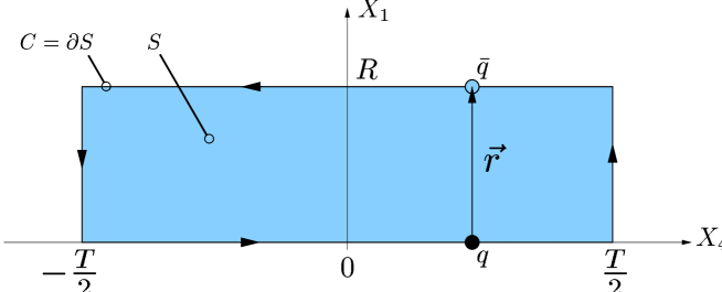
Figure 1: A static color dipole of size $R$ in the fundamental representation. The rectangular path $C$ of spatial extension $R$ and temporal extension $T$ indicates the world-line of the dipole described the Wegner-Wilson loop $W_{\mbox{\scriptsize N}_{c}}[C]$. The shaded area bounded by the loop $C=\partial S$ represents the minimal surface $S$ used to compute the static dipole potential.

illustrates a static color dipole in the fundamental representation $r=\mbox{N}_{c}$. The potential of the static color dipole is obtained from the VEV of the corresponding Wegner-Wilson loop [15, 65]

$$V_{r}(R)=-\lim_{T\to\infty}\frac{1}{T}\ln\langle W_{r}[C]\rangle_{\mbox{\scriptsize pot}}\ ,$$ (3.1)

where “pot” indicates the subtraction of the self-energy of the color sources. This subtraction corresponds to the mass renormalization of the heavy color sources as discussed above. The static quark-antiquark potential $V_{\mbox{\scriptsize N}_{c}}$ is obtained from a loop in the fundamental representation ($r\!=\!\mbox{N}_{c}$) and the potential of a static gluino pair $V_{\mbox{\scriptsize N}_{c}^{2}\!-\!1}$ from a loop in the adjoint representation ($r\!=\!\mbox{N}_{c}^{2}\!-\!1$).

With our result for $\langle W_{r}[C]\rangle$, (2.14), obtained with the Gaussian approximation in the gluon field strength, the static potential reads

$$V_{r}(R)=\frac{C_{2}(r)}{2}\,\lim_{T\to\infty}\frac{1}{T}\,\chi_{SS\,\mbox{\scriptsize pot}}$$ (3.2)

with the self-energy subtracted, i.e. $\chi_{SS\,\mbox{\scriptsize pot}}:=\chi_{SS}-\chi_{SS\,\mbox{\scriptsize self}}$ (see Appendix C). According to the structure of the gluon field strength correlator, (2.12) and (2.42), there are perturbative ($P$) and non-perturbative ($N\!P$) contributions to the static potential:

$$V_{r}(R)=\frac{C_{2}(r)}{2}\,\lim_{T\to\infty}\frac{1}{T}\,\left\{\chi_{SS\,\mbox{\scriptsize pot}}^{P}+\left(\chi_{SS\,\mbox{\scriptsize pot}}^{N\!P\,\,nc}+\chi_{SS\,\mbox{\scriptsize pot}}^{N\!P\,\,c}\right)\right\}\ ,$$ (3.3)

where the explicit form of the $\chi$ functions is given in (C.9), (C.28), and (C.37).

The perturbative contribution to the static potential describes the color Yukawa potential (which reduces to the color Coulomb potential [66] for $m_{G}=0$)

$$V_{r}^{P}(R)=-C_{2}(r)\,\frac{g^{2}(R)}{4\pi R}\exp[-m_{G}R]\ .$$ (3.4)

Here we have used the result for $\chi_{SS\,\mbox{\scriptsize pot}}^{P}$ given in (C.37) and the perturbative correlation function

$$D^{\prime\,(3)}_{P}(\vec{Z}^{2}):=\int\frac{d^{4}K}{(2\pi)^{3}}\,e^{iKZ}\,\tilde{D}^{\prime\,(3)}_{P}(K^{2})\,\delta(K_{4})=-\,\frac{\exp[-\,m_{G}\,|\vec{Z}|]}{4\pi|\vec{Z}|}$$ (3.5)

which is obtained from the massive gluon propagator (2.43). As shown below, the perturbative contribution dominates the static potential for small dipole sizes $R$.

The non-perturbative contributions to the static potential, the non-confining component ($nc$) and the confining component ($c$), read

$$V_{r}^{N\!P\,\,nc}(R) = C_{2}(r)\,\,\frac{\pi^{2}G_{2}(1-\kappa)}{3(N_{c}^{2}-1)}\,\,D_{1}^{\prime\,(3)}(R^{2})\ ,$$ (3.6)

$$V_{r}^{N\!P\,\,c}(R) = C_{2}(r)\,\,\frac{\pi^{2}G_{2}\kappa}{3(N_{c}^{2}-1)}\,\,\int_{0}^{R}\!\!d\rho\,(R-\rho)\,D^{(3)}(\rho^{2})\ ,$$ (3.7)

where we have used the results for $\chi_{SS\,\mbox{\scriptsize pot}}^{N\!P\,\,nc}$ and $\chi_{SS\,\mbox{\scriptsize pot}}^{N\!P\,\,c}=\chi_{SS}^{N\!P\,\,c}$ given respectively in (C.28) and (C.9) obtained with the minimal surface, i.e. the planar surface bounded by the loop as indicated by the shaded area in Fig. 1. With the exponential correlation function (2.50), the correlation functions in (3.6) and (3.7) read

$$D^{\prime\,(3)}_{1}(\vec{Z}^{2}) \!\!:=\!\! \int\frac{d^{4}K}{(2\pi)^{3}}\,e^{iKZ}\,\tilde{D}^{\prime\,(3)}_{1}(K^{2})\,\delta(K_{4})\,\,=\,\,-\,a\,|\vec{Z}|^{2}\,K_{2}[|\vec{Z}|/a]\ ,$$ (3.8)

$$D^{(3)}(\vec{Z}^{2}) \!\!:=\!\! \int\frac{d^{4}K}{(2\pi)^{3}}\,e^{iKZ}\,\tilde{D}(K^{2})\,\delta(K_{4})\,\,=\,\,2\,|\vec{Z}|\,K_{1}[|\vec{Z}|/a]\ .$$ (3.9)

For large dipole sizes, $R\gtrsim 0.5\ \mbox{fm}$, the non-confining contribution (3.6) vanishes exponentially while the confining contribution (3.7)—as anticipated—leads to confinement [21], i.e. the confining linear increase,

$$V_{r}^{N\!P\,\,c}(R)\Big{|}_{R\,\gtrsim\,0.5\,\mbox{\scriptsize fm}}=\sigma_{r}R+\mbox{const.}$$ (3.10)

Thus, the QCD string tension is given by the confining SVM component [21]: For a color dipole in the $SU(N_{c})$ representation $r$, it reads

$$\sigma_{r}=C_{2}(r)\,\,\frac{\pi^{3}G_{2}\kappa}{48}\int_{0}^{\infty}dZ^{2}D(Z^{2})=C_{2}(r)\,\,\frac{\pi^{3}\kappa G_{2}a^{2}}{24}\ ,$$ (3.11)

where the exponential correlation function (2.50) is used in the final step. Since the string tension can be computed from first principles within lattice QCD [64], relation (3.11) puts an important constraint on the three parameters of the non-perturbative QCD vacuum $a$, $G_{2}$, and $\kappa$. With the values for $a$, $G_{2}$, and $\kappa$ given in (2.51), which are used throughout this work, one obtains for the string tension of the $SU(3)$ quark-antiquark potential ($r=3$) a reasonable value of

$$\sigma_{3}=0.22\,\mbox{GeV}^{2}\equiv 1.12\,\mbox{GeV}/\mbox{fm}\ .$$ (3.12)

The static $SU(N_{c}=3)$ quark-antiquark potential $V_{\mbox{\scriptsize N}_{c}}(R)=V_{3}(R)$ is shown as a function of the quark-antiquark separation $R$ in Fig. 2,

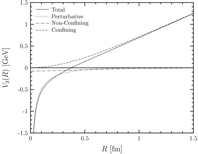
Figure 2: The static $SU(N_{c}=3)$ quark-antiquark potential $V_{\mbox{\scriptsize N}_{c}}(R)=V_{3}(R)$ as a function of the quark-antiquark separation $R$. The solid, dotted, and dashed lines indicate the full static potential and its perturbative and non-perturbative contributions, respectively. For small quark-antiquark separations, $R\lesssim 0.5\,\mbox{fm}$, the perturbative contribution dominates and gives rise to the well-known color Coulomb behavior at small distances. For medium and large quark-antiquark separations, $R\gtrsim 0.5\,\mbox{fm}$, the non-perturbative contribution dominates and leads to the confining linear rise of the static potential. As our model is working in the quenched approximation, string breaking cannot be described, which is expected to stop the linear increase for $R\,\gtrsim\,1\,\mbox{fm}$ [67, 64].

where the solid, dotted, and dashed lines indicate the full static potential and its perturbative and non-perturbative contributions, respectively. For small quark-antiquark separations $R\lesssim 0.5\,\mbox{fm}$, the perturbative contribution dominates giving rise to the well-known color Coulomb behavior. For medium and large quark-antiquark separations $R\gtrsim 0.5\,\mbox{fm}$, the non-perturbative contribution dominates and leads to the confining linear rise of the static potential. The transition from perturbative to string behavior takes place at source separations of about $0.5\,\mbox{fm}$ in agreement with the recent results of Lüscher and Weisz [26]. This supports our value for the gluon mass $m_{G}=m_{\rho}=0.77\,\mbox{GeV}$ which is important only around $R\approx 0.4\,\mbox{fm}$, i.e. for the interplay between perturbative and non-perturbative physics. For $R\lesssim 0.3\,\mbox{fm}$ and $R\gtrsim 0.5\,\mbox{fm}$, the effect of the gluon mass, introduced as an IR regulator in our perturbative component, is negligible. String breaking is expected to stop the linear increase for $R\,\gtrsim\,1\,\mbox{fm}$ where lattice investigations show deviations from the linear rise in full QCD [67, 64]. As our model is working in the quenched approximation, string breaking through dynamical quark-antiquark production is excluded.

As can be seen from (3.2), the static potential shows Casimir scaling which emerges in our approach as a trivial consequence of the Gaussian approximation used to truncate the cumulant expansion (2.7). Indeed, the Casimir scaling hypothesis [68] has been verified to high accuracy for $SU(3)$ on the lattice [19, 20] (see also Fig. 3). These lattice results have been interpreted as a strong hint toward Gaussian dominance in the QCD vacuum and thus as evidence for a strong suppression of higher cumulant contributions [69, 70]. In contrast to our model, the instanton model can describe neither Casimir scaling [70] nor the linear rise of the confining potential [71].

Figure 3

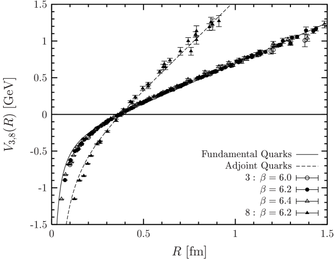
Figure 3: The static $SU(N_{c}=3)$ potential of color dipoles in the fundamental representation $V_{3}(R)$ (solid line) and adjoint representation $V_{8}(R)$ (dashed line) as a function of the dipole size $R$ in comparison to $SU(3)$ lattice data for $\beta=6.0$, 6.2, and 6.4 [20, 64]. The model results are in good agreement with the lattice data. This particularly holds for the obtained Casimir scaling behavior.

shows the static $SU(N_{c}=3)$ potential for fundamental sources $V_{\mbox{\scriptsize N}_{c}}(R)=V_{3}(R)$ (solid line) and adjoint sources $V_{\mbox{\scriptsize N}_{c}^{2}\!-\!1}(R)=V_{8}(R)$ (dashed line) as a function of the dipole size $R$ in comparison to $SU(3)$ lattice data [20, 64]. The model results are in good agreement with the lattice data. In particular, the obtained Casimir scaling behavior is strongly supported by $SU(3)$ lattice data [19, 20]. This, however, points also to a shortcoming of our model: From Eq. (3.2) and Fig. 3 it is clear that string breaking is described neither for fundamental nor for adjoint dipoles in our model which indicates that not only dynamical fermions (quenched approximation) but also some gluon dynamics are missing.

An extension of the model that allows one to describe color screening remains a major challenge. Without such a modification, our model unfortunately cannot contribute to the recent discussion on the scaling behavior of $k$-string tensions $\sigma_{k}$, i.e. the tensions of strings connecting sources with $\cal{N}$-ality $k\geq 1$. A source of $\cal{N}$-ality $k\leq N_{c}/2$ is defined as a source in the representation constructed from the tensor product of quarks—objects transforming under the fundamental representation—and antiquarks—objects transforming under the conjugated representation—where $k$ is the number of quarks minus the number of antiquarks modulo $N_{c}$; see e.g. [72]. For $SU(N_{c})$ with $N_{c}\geq 4$, $k$ strings are particularly interesting since in addition to the fundamental ($k=1$) string other strings also exist that are stable against color screening. Based on lattice results for $N_{c}=4,5,6$ [72, 73], the present debate is whether the corresponding string tensions show Casimir scaling behavior $\sigma_{k}\propto k(N_{c}-k)$ , the sine law behavior $\sigma_{k}\propto\sin(\pi k/N_{c})$ predicted from M-theory approaches to QCD [74], or simply the behavior of $k$ non-interacting fundamental strings $\sigma_{k}=k\sigma_{\mbox{\scriptsize N}_{c}}$. Physical explanations of the lattice results obtained are discussed, for example, in the center vortex confinement mechanism [75, 7].

4 Chromo-Field Distributions of Color Dipoles

In this section we compute the chromo-electric fields generated by a static color dipole in the fundamental and adjoint representation of $SU(N_{c})$. We find formation of a color flux tube that confines the two color sources in the dipole. This confining string is analyzed quantitatively. Its mean squared radius is calculated and transverse and longitudinal energy density profiles are provided. The interplay between perturbative and non-perturbative contributions to the chromo-field distributions is investigated and exact Casimir scaling is found for both contributions.

As already explained in Sec. 3, the static color dipole—two static color sources separated by a distance $R$ in a net color singlet state—is described by a Wegner-Wilson loop $W_{r}[C]$ with a rectangular path $C$ of spatial extension $R$ and temporal extension $T\to\infty$ (cf. Fig. 1) where $r$ indicates the $SU(N_{c})$ representation of the sources considered. A second small quadratic loop or plaquette in the fundamental representation placed at the space-time point $X$ with side length $R_{P}\to 0$ and oriented along the $\alpha\beta$ axes,

$$P_{\mbox{\scriptsize N}_{c}}^{\alpha\beta}(X)=\tilde{\mbox{Tr}}_{\mbox{\scriptsize N}_{c}}\exp\!\!\left[-ig\oint_{C_{P}}\!\!\!dZ_{\mu}{\cal G}_{\mu}^{a}(Z)t_{\mbox{\scriptsize N}_{c}}^{a}\right]=1-R_{P}^{4}\frac{g^{2}}{4N_{c}}{\cal G}_{\alpha\beta}^{a}(X){\cal G}_{\alpha\beta}^{a}(X)+{\cal O}(R_{P}^{6})\ ,$$ (4.1)

is needed—as a “Hall probe”—to calculate the chromo-field distributions at the space-time point $X$ caused by the static sources [76, 77]

$$\Delta G_{r\,\alpha\beta}^{2}(X) := \Big{\langle}\frac{g^{2}}{4\pi^{2}}{\cal G}_{\alpha\beta}^{a}(X){\cal G}_{\alpha\beta}^{a}(X)\Big{\rangle}_{W_{r}[C]}-\Big{\langle}\frac{g^{2}}{4\pi^{2}}{\cal G}_{\alpha\beta}^{a}(X){\cal G}_{\alpha\beta}^{a}(X)\Big{\rangle}_{\mbox{\scriptsize vac}}$$ (4.2)

$$= -\,\lim_{R_{P}\to 0}\frac{1}{R_{P}^{4}}\frac{N_{c}}{\pi^{2}}\left[\frac{\langle W_{r}[C]P_{\mbox{\scriptsize N}_{c}}^{\alpha\beta}(X)\rangle}{\langle W_{r}[C]\rangle}-\langle P_{\mbox{\scriptsize N}_{c}}^{\alpha\beta}(X)\rangle\right]$$ (4.3)

with no summation over $\alpha$ and $\beta$ in (4.1), (4.2), and (4.3). In definition (4.2) $\langle\ldots\rangle_{W_{r}[C]}$ indicates the VEV in the presence of the static color dipole while $\langle\ldots\rangle_{\mbox{\scriptsize vac}}$ indicates the VEV in the absence of any color sources. Depending on the plaquette orientation indicated by $\alpha$ and $\beta$, one obtains from (4.3) the squared components of the chromo-electric and chromo-magnetic fields at the space-time point $X$:

$$\Delta G_{r\,\alpha\beta}^{2}(X)=\frac{g^{2}}{4\pi^{2}}\left(\begin{array}[]{cccc}0&B_{z}^{2}&B_{y}^{2}&E_{x}^{2}\\ B_{z}^{2}&0&B_{x}^{2}&E_{y}^{2}\\ B_{y}^{2}&B_{x}^{2}&0&E_{z}^{2}\\ E_{x}^{2}&E_{y}^{2}&E_{z}^{2}&0\end{array}\right)(X)\ ,$$ (4.4)

i.e. space-time plaquettes ($\alpha\beta=i4$) measure chromo-electric fields and space-space plaquettes ($\alpha\beta=ij$) chromo-magnetic fields. As shown in Fig. 4, we place the static color sources on the $X_{1}$ axis at $(X_{1}=\pm R/2,0,0,X_{4})$ and use the following notation plausible from symmetry arguments

$$E_{\parallel}^{2}=E_{x}^{2}\ ,\quad E_{\perp}^{2}=E_{y}^{2}=E_{z}^{2}\ ,\quad B_{\parallel}^{2}=B_{x}^{2}\ ,\quad B_{\perp}^{2}=B_{y}^{2}=B_{z}^{2}\ .$$ (4.5)

Figure 4 illustrates also the plaquette $P_{\mbox{\scriptsize N}_{c}}^{14}(X)$ at $X=(X_{1},X_{2},0,0)$ needed to compute $E_{\parallel}^{2}(X)$. Due to symmetry arguments, the complete information on the chromo-field distributions is obtained from plaquettes in “transverse” space $X=(X_{1},X_{2},0,0)$ with four different orientations, $\alpha\beta=14,\,24,\,13,\,23$ [cf. Eq. (4.5)].

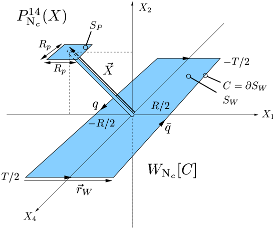
Figure 4: The plaquette-loop geometry needed to compute the squared chromo-electric field $E_{\parallel}^{2}(X)$ generated by a static color dipole in the fundamental $SU(N_{c})$ representation ($r=\mbox{N}_{c}$). The rectangular path $C$ indicates the world-line of the static dipole described the Wegner-Wilson loop $W_{\mbox{\scriptsize N}_{c}}[C]$. The square with side length $R_{P}$ illustrates the plaquette $P_{\mbox{\scriptsize N}_{c}}^{14}(X)$. The shaded areas represent the minimal surfaces used in our computation of the chromo-field distributions. The thin tube allows us to compare the gluon field strengths in surface $S_{P}$ with the gluon field strengths in surface $S_{W}$.

The energy and action density distributions around a static color dipole in the $SU(N_{c})$ representation $r$ are given by the squared chromo-field distributions

$$\varepsilon_{r}(X) = \frac{1}{2}\left[-\vec{E}^{2}(X)+\vec{B}^{2}(X)\right]$$ (4.6)

$$\mathit{s}_{r}(X) = -\frac{1}{2}\left[\vec{E}^{2}(X)+\vec{B}^{2}(X)\right]$$ (4.7)

with signs according to Euclidean space-time conventions. Low-energy theorems that relate the energy and action stored in the chromo-fields of the static color dipole to the corresponding ground state energy are discussed in the next section.

For the chromo-field distributions of a static color dipole in the fundamental representation of $SU(N_{c})$, i.e. a static quark-antiquark pair, we obtain with our results for the VEV of one loop (2.14) and the correlation of two loops in the fundamental representation (2.35)

$$\Delta G_{\mbox{\scriptsize N}_{c}\,\alpha\beta}^{2}(X)=-\lim_{R_{P}\to 0}\frac{1}{R_{P}^{4}}\frac{N_{c}}{\pi^{2}}\exp\left[-\frac{C_{2}(\!\mbox{N}_{c}\!)}{2}\,\chi_{S_{P}S_{P}}\right]$$ (4.8)

$$\hskip 56.9055pt\times\Bigg{(}\frac{N_{c}+1}{2N_{c}}\exp\!\left[-\frac{N_{c}-1}{2N_{c}}\chi_{S_{P}S_{W}}\right]+\frac{N_{c}-1}{2N_{c}}\exp\!\left[\frac{N_{c}+1}{2N_{c}}\chi_{S_{P}S_{W}}\right]-1\Bigg{)}$$

where $\chi_{S_{i}S_{j}}$ is defined in (2.27). The subscripts $P$ and $W$ indicate surface integrations to be performed over the surfaces spanned by the plaquette and the Wegner-Wilson loop, respectively. Choosing the surfaces—as illustrated by the shaded areas in Fig. 4—to be the minimal surfaces connected by an infinitesimal thin tube (which gives no contribution to the integrals) it is clear that $\chi_{S_{P}S_{P}}\propto R_{P}^{4}$ and $\chi_{S_{P}S_{W}}\propto R_{P}^{2}$. Being interested in the chromo-fields at the space-time point $X$, the extension of the quadratic plaquette is taken to be infinitesimally small, $R_{P}\rightarrow 0$, so that one can expand the exponential functions and keep only the term of lowest order in $R_{P}$:

$$\Delta G_{\mbox{\scriptsize N}_{c}\,\alpha\beta}^{2}(X)=-\,C_{2}(\!\mbox{N}_{c}\!)\,\lim_{R_{P}\to 0}\frac{1}{R_{P}^{4}}\,\frac{1}{4\pi^{2}}\,\chi_{S_{P}S_{W}}^{2}\ .$$ (4.9)

This result—obtained with the matrix cumulant expansion in a very straightforward way—agrees exactly with the result derived in [25] with the expansion method. Indeed, the expansion method agrees for small $\chi$ functions with the matrix cumulant expansion (Berger-Nachtmann approach) used in this work but breaks down for large $\chi$ functions, where the matrix cumulant expansion is still applicable.

The chromo-field distributions of a static color dipole in the adjoint representation of $SU(N_{c})$, i.e. a static gluino pair, are computed analogously. Using our result (2.40) for the correlation of one loop in the fundamental representation (plaquette) with one loop in the adjoint representation (static sources), one obtains

$$\!\!\!\!\!\!\!\!\Delta G_{\mbox{\scriptsize N}_{c}^{2}\!-\!1\,\alpha\beta}^{2}(X)=-\lim_{R_{P}\to 0}\frac{1}{R_{P}^{4}}\frac{N_{c}}{\pi^{2}}\exp\left[-\frac{C_{2}(\!\mbox{N}_{c}\!)}{2}\chi_{S_{P}S_{P}}\right]\,\Bigg{(}\!\frac{1}{N_{c}^{2}\!-\!1}\,\exp\!\Big{[}\frac{N_{c}}{2}\,\chi_{S_{P}S_{W}}\Big{]}$$

$$\hskip 42.67912pt+\,\frac{N_{c}\!+\!2}{2(N_{c}\!+\!1)}\exp\!\Big{[}\!-\frac{1}{2}\,\chi_{S_{P}S_{W}}\Big{]}+\frac{N_{c}\!-\!2}{2(N_{c}\!-\!1)}\exp\!\Big{[}\frac{1}{2}\,\chi_{S_{P}S_{W}}\Big{]}-1\!\Bigg{)}$$ (4.10)

which reduces—as explained for sources in the fundamental representation—to

$$\Delta G_{\mbox{\scriptsize N}_{c}^{2}\!-\!1\,\alpha\beta}^{2}(X)=-\,C_{2}(\!\mbox{N}_{c}^{2}\!-\!1\!)\,\lim_{R_{P}\to 0}\frac{1}{R_{P}^{4}}\,\frac{1}{4\pi^{2}}\,\chi_{S_{P}S_{W}}^{2}\ .$$ (4.11)

Thus, the squared chromo-electric fields of an adjoint dipole differ from those of a fundamental dipole only in the eigenvalue of the corresponding quadratic Casimir operator $C_{2}(r)$. In fact, Casimir scaling of the chromo-field distributions holds for dipoles in any representation $r$ of $SU(N_{c})$ in our model. As can be seen with the low-energy theorems discussed below, this is in line with the Casimir scaling of the static dipole potential found in the previous section. In addition to lattice investigations that show Casimir scaling of the static dipole potential to high accuracy in $SU(3)$ [19, 20], Casimir scaling of the chromo-field distributions has been considered on the lattice as well but only for $SU(2)$ [78]. Here only slight deviations from the Casimir scaling hypothesis have been found which were interpreted as hints toward adjoint quark screening.

In our model the shape of the field distributions around the color dipole is identical for all $SU(N_{c})$ representations $r$ and given by $\chi_{S_{P}S_{W}}^{2}$. This again illustrates the shortcoming of our model discussed in the previous section. Working in the quenched approximation, one expects a difference between fundamental and adjoint dipoles: string breaking cannot occur in fundamental dipoles as dynamical quark-antiquark production is excluded but should be present for adjoint dipoles because of gluonic vacuum polarization. Comparing (4.9) with (4.11) it is clear that this difference is not described in our model. In fact, as shown in Sec. 3, string breaking is described neither for fundamental nor for adjoint dipoles. Interestingly, even on the lattice there has been no striking evidence for adjoint quark screening in quenched QCD [79]. It is even conjectured that the Wegner-Wilson loop operator is not suited to studies of string breaking [80].

In the LLCM there are perturbative ($P$) and non-perturbative ($N\!P$) contributions to the chromo-electric fields according to the structure of the gluon field strength correlator, (2.12) and (2.42),

$$\Delta G_{r\,\alpha\beta}^{2}(X) = -C_{2}(r)\,\lim_{R_{P}\to 0}\frac{1}{R_{P}^{4}}\,\frac{1}{\pi^{2}}\,$$

$$\times\left(\left[\chi_{S_{P}S_{W}}^{P}(X)\right]_{\alpha\beta}^{2}+\left\{\left[\chi_{S_{P}S_{W}}^{N\!P\,nc}(X)\right]_{\alpha\beta}+\left[\chi_{S_{P}S_{W}}^{N\!P\,c}(X)\right]_{\alpha\beta}\right\}^{2}\right)\ .$$

Interference of perturbative and non-perturbative correlations is not considered to be in line with the applications of our model to high-energy scattering [8, 32, 33, 34] with separate hard (perturbative) and soft (non-perturbative) Pomeron exchanges. The interferences do not change the qualitative picture. Slight modifications occur in regions where fields originating from perturbative and non-perturbative correlations are of similar size. For the $\chi$ functions in (4), we give directly in the following the final results obtained with the minimal surfaces shown in Fig. 4. Details of their derivation can be found in Appendix C.

The perturbative contribution ($P$) described by massive gluon exchange leads, of course, to the well-known color Yukawa field which reduces to the color Coulomb field for $m_{G}=0$. It contributes only to the chromo-electric fields, $E_{\parallel}^{2}=E_{x}^{2}$ ($\alpha\beta=14$) and $E_{\perp}^{2}=E_{y}^{2}=E_{z}^{2}$ ($\alpha\beta=24$), and reads explicitly for $X=(X_{1},X_{2},0,0)$

$$\!\!\!\!\!\!\!\!\!\!\!\!\left[\chi_{S_{P}S_{W}}^{P}(X)\right]_{14} \!\!=\!\! -\,\frac{R_{P}^{2}}{2}\!\int_{-\infty}^{\infty}\!\!\!d\tau\left\{(X_{1}-R/2)\,g^{2}(Z_{1A}^{2})\,D_{P}(Z_{1A}^{2})\right.$$ (4.13)

$$\hphantom{-\,\frac{R_{P}^{2}}{2}\!\int_{-\infty}^{\infty}\!\!\!d\tau\Big{(}}\left.-\,(X_{1}+R/2)\,g^{2}(Z_{1C}^{2})\,D_{P}(Z_{1C}^{2})\right\}$$

$$\!\!\!\!\!\!\!\!\!\!\!\!\left[\chi_{S_{P}S_{W}}^{P}(X)\right]_{24} \!\!=\!\! -\,\frac{R_{P}^{2}}{2}\!\int_{-\infty}^{\infty}\!\!\!d\tau\,X_{2}\left\{g^{2}(Z_{1A}^{2})\,D_{P}(Z_{1A}^{2})-g^{2}(Z_{1C}^{2})\,D_{P}(Z_{1C}^{2})\right\}$$ (4.14)

with the perturbative correlation function (2.45), the running coupling (2.47), and

$$Z_{1A}^{2}=\left(X_{1}\!-\!\frac{R}{2}\right)^{2}+X_{2}^{2}+\tau^{2}\quad\mbox{and}\quad Z_{1C}^{2}=\left(X_{1}\!+\!\frac{R}{2}\right)^{2}+X_{2}^{2}+\tau^{2}\ .$$ (4.15)

The non-confining non-perturbative contribution ($N\!P\,nc$) has the same structure as the perturbative contribution—as expected from the identical tensor structure—but differs, of course, in the prefactors and the correlation function, $D_{1}\neq D_{p}$. Its contributions to the chromo-electric fields $E_{\parallel}^{2}=E_{x}^{2}$ ($\alpha\beta=14$) and $E_{\perp}^{2}=E_{y}^{2}=E_{z}^{2}$ ($\alpha\beta=24$) read for $X=(X_{1},X_{2},0,0)$

$$\left[\chi_{S_{P}S_{W}}^{N\!P\,\,nc}(X)\right]_{14} = -\,\frac{R_{P}^{2}\pi^{2}G_{2}(1\!-\!\kappa)}{6\,(N_{c}^{2}\!-\!1)}\!\int_{-\infty}^{\infty}\!\!\!d\tau\Big{\{}(X_{1}-R/2)\,D_{1}(Z_{1A}^{2})$$ (4.16)

$$\hphantom{-\,\frac{R_{P}^{2}\pi^{2}G_{2}}{6\,(N_{c}^{2}\!-\!1)}}-\,(X_{1}+R/2)\,D_{1}(Z_{1C}^{2})\Big{\}}$$

$$\left[\chi_{S_{P}S_{W}}^{N\!P\,\,nc}(X)\right]_{24} = -\,\frac{R_{P}^{2}\pi^{2}G_{2}(1\!-\!\kappa)}{6\,(N_{c}^{2}\!-\!1)}\!\int_{-\infty}^{\infty}\!\!\!d\tau\,X_{2}\Big{\{}D_{1}(Z_{1A}^{2})-D_{1}(Z_{1C}^{2})\Big{\}}$$ (4.17)

with the exponential correlation function (2.50) and $Z_{1A}^{2}$ and $Z_{1C}^{2}$ as given in (4.15).

The confining non-perturbative contribution ($N\!P\,c$) has a different structure that leads to confinement and flux-tube formation. It gives contributions only to the chromo-electric field $E_{\parallel}^{2}=E_{x}^{2}$ ($\alpha\beta=14$) which read for $X=(X_{1},X_{2},0,0)$

$$\left[\chi_{S_{P}S_{W}}^{N\!P\,\,c}(X)\right]_{14} = R_{P}^{2}R\frac{\pi^{2}G_{2}\kappa}{3\,(N_{c}^{2}\!-\!1)}\int_{0}^{1}d\rho\,D^{(3)}(\vec{Z_{\perp}}^{2})\ ,$$ (4.18)

with the correlation function given in (3.9) as derived from the exponential correlation function (2.50), and

$$\vec{Z}_{\perp}^{2}=[X_{1}+(1/2-\rho)R]^{2}+X_{2}^{2}\ .$$ (4.19)

In our model there are no contributions to the chromo-magnetic fields, i.e. the static color charges do not affect the magnetic background field

$$B_{\parallel}^{2}=B_{x}^{2}=0\quad\mbox{and}\quad B_{\perp}^{2}=B_{y}^{2}=B_{z}^{2}=0\ ,$$ (4.20)

which can be seen from the corresponding plaquette-loop geometries as pointed out in Appendix C. Thus, the energy and action densities are identical in our approach and completely determined by the squared chromo-electric fields

$$\varepsilon_{r}(X)\,\,=\,\,\mathit{s}_{r}(X)\,\,=\,\,-\frac{1}{2}\,\vec{E}^{2}(X)\ .$$ (4.21)

This picture is in agreement with other effective theories of confinement such as the ’t Hooft–Mandelstam picture [81] or dual QCD [82] and, indeed, a relation between the dual Abelian Higgs model and the SVM has been established [83]. In contrast, lattice investigations work at scales at which the chromo-electric and chromo-magnetic fields are of similar magnitude [84, 85, 30, 86]. Indeed, these simulations have been performed in $SU(N_{c}=2)$ at bare couplings $g^{2}_{0}$ down to $\beta_{0}=4/g^{2}_{0}=2.74$ corresponding to a minimum lattice cutoff of $0.04\,\mbox{fm}$, which determines also the minimum size of the plaquette used in the measurements of the color fields. Interestingly, as shown in Figs. 13 and 14 of [84], the action density slightly decreases by decreasing the lattice spacing from $0.08\,\mbox{fm}$ ($\beta_{0}=2.5$) to $0.05\,\mbox{fm}$ ($\beta_{0}=2.635$). In our model the vanishing of the chromo-magnetic fields determines the value of the Callan-Symanzik $\beta$ function at the renormalization scale at which our non-perturbative component is working. This is shown as a result of low-energy theorems in the next section.

In Fig. 5 the energy density distributions $g^{2}\varepsilon_{3}(X_{1},X_{2}\!=\!X_{3})$ generated by a color dipole in the fundamental $SU(N_{c}=3)$ representation ($r\!=\!3$) are shown for quark-antiquark separations of $R=0.1,\,0.5,\,1$ and $1.5\,\mbox{fm}$. With increasing dipole size $R$, one sees explicitly the formation of the flux tube which represents the confining QCD string.

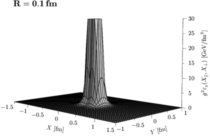
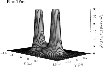
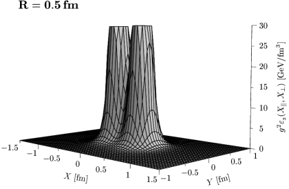
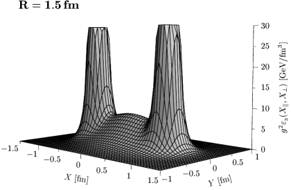
Figure 5: Energy density distributions $g^{2}\varepsilon_{3}(X_{1},X_{2}\!=\!X_{3})$ generated by a color dipole in the fundamental $SU(3)$ representation ($r\!=\!3$) for quark-antiquark separations of $R=0.1,\,0.5,\,1$ and $1.5\,\mbox{fm}$. Flux-tube formation leads to the confining QCD string with increasing dipole size $R$.

The longitudinal and transverse energy density profiles generated by a color dipole in the fundamental representation ($r=3$) of $SU(N_{c}=3)$ are shown for quark-antiquark separations (dipole sizes) of $R=0.1,\,0.5,\,1$ and $1.5\,\mbox{fm}$ in Figs. 6 and 7. The perturbative and non-perturbative contributions are given by the dotted and dashed lines, respectively, and the sum of both in the solid lines. The open and filled circles indicate the quark and antiquark positions. As can be seen from (4.3) and (4.4), we cannot compute the energy density separately but only the product $g^{2}\varepsilon_{r}(X)$. Nevertheless, a comparison of the total energy stored in chromo-electric fields to the ground state energy of the color dipole via low-energy theorems yields $g^{2}=10.2$ $(\equiv\alpha_{s}=0.81)$ for the non-perturbative SVM component as shown in the next section.

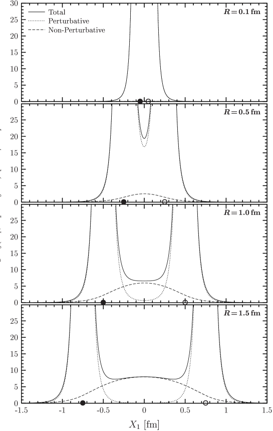
Figure 6: Longitudinal energy density profiles $g^{2}\varepsilon_{3}(X_{1},X_{2}\!=\!X_{3}\!=\!0)$ generated by a color dipole in the fundamental $SU(3)$ representation ($r\!=\!3$) for quark-antiquark separations of $R=0.1,\,0.5,\,1$ and $1.5\,\mbox{fm}$. The dotted and dashed lines give the perturbative and non-perturbative contributions, respectively, and the solid lines the sum of both. The open and filled circles indicate the quark and antiquark positions. For small dipoles, $R=0.1\,\mbox{fm}$, perturbative physics dominates and non-perturbative correlations are negligible. For large dipoles, $R\gtrsim 1\,\mbox{fm}$, the formation the confining string (flux tube) can be seen which dominates the chromo-electric fields between the color sources.

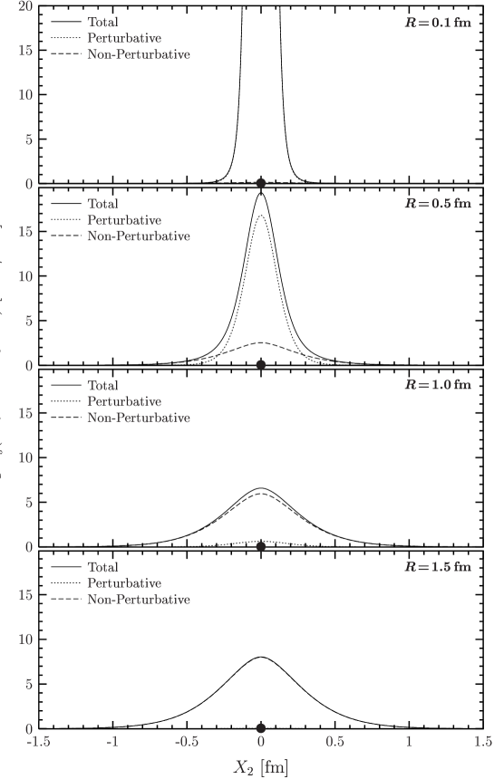
Figure 7: Transverse energy density profiles $g^{2}\varepsilon_{3}(X_{2},X_{1}\!=\!X_{3}\!=\!0)$ generated by a color dipole in the fundamental $SU(3)$ representation ($r\!=\!3$) for quark-antiquark separations of $R=0.1,\,0.5,\,1$ and $1.5\,\mbox{fm}$. The dotted and dashed lines give the perturbative and non-perturbative contributions, respectively, and the solid lines the sum of both. The filled circles indicate the positions of the color sources. For small dipoles, $R=0.1\,\mbox{fm}$, perturbative physics dominates and non-perturbative correlations are negligible. For large dipoles, $R\gtrsim 1\,\mbox{fm}$, the formation the confining string (flux tube) can be seen which dominates the chromo-electric fields between the color sources.

In Figs. 6 and 7 the formation of the confining string (flux tube) with increasing source separations $R$ can again be seen explicitly: For small dipoles, $R=0.1\,\mbox{fm}$, perturbative physics dominates and non-perturbative correlations are negligible. For large dipoles, $R\gtrsim 1\,\mbox{fm}$, the non-perturbative correlations lead to formation of a narrow flux tube which dominates the chromo-electric fields between the color sources.

Figure 8

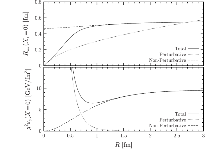
Figure 8: Root mean squared radius $R_{ms}$ of the flux tube and energy density in the center of a fundamental $SU(3)$ dipole $g^{2}\varepsilon_{3}(X=0)$ as a function of the dipole size $R$. Perturbative and non-perturbative contributions are given respectively by the dotted and dashed lines and the sum of both in the solid lines. For large $R$, both the width and height of the flux tube in the central region are governed completely by non-perturbative physics and saturate respectively at $R_{ms}^{R\to\infty}\approx 0.55\,\mbox{fm}$ and $\varepsilon_{3}^{R\to\infty}(X=0)\approx 1\,\mbox{GeV}/\mbox{fm}^{3}$. The latter value is extracted with the result $g^{2}=10.2$ deduced from low-energy theorems in the next section.

shows the evolution of the transverse width (upper plot) and height (lower plot) of the flux tube in the central region of the Wegner-Wilson loop as a function of the dipole size $R$ where perturbative and non-perturbative contributions are given by the dotted and dashed lines, respectively, and the sum of both in the solid lines. The width of the flux tube is best described by the root mean squared ($ms$) radius

$$R_{ms}=\sqrt{\frac{\int dX_{\perp}\,X_{\perp}^{3}\,g^{2}\varepsilon_{r}(X_{1}=0,X_{\perp})}{\int dX_{\perp}\,X_{\perp}\,g^{2}\varepsilon_{r}(X_{1}=0,X_{\perp})}}\ ,$$ (4.22)

which is universal for dipoles in all $SU(N_{c})$ representations $r$ as the Casimir factors divide out. The height of the flux tube is given by the energy density in the center of the considered dipole, $g^{2}\varepsilon_{r}(X=0)$. For large source separations, $R\gtrsim 1\,\mbox{fm}$, both the width and height of the flux tube in the central region of the Wegner-Wilson loop are governed completely by non-perturbative physics and saturate for a fundamental $SU(3)$ dipole ($r=\mbox{N}_{c}=3$) at reasonable values of

$$R_{ms}^{R\to\infty}\approx 0.55\,\mbox{fm}\quad\mbox{and}\quad\varepsilon_{3}^{R\to\infty}(X=0)\approx 1\,\mbox{GeV}/\mbox{fm}^{3}\quad\mbox{with}\quad g^{2}=10.2\ .$$ (4.23)

Note that the qualitative features of the non-perturbative SVM component do not depend on the specific choice for the parameters, surfaces, and correlation functions and have already been discussed with the pyramid mantle choice of the surface and different correlation functions in the first investigation of flux-tube formation in the SVM [25]. The quantitative results, however, are sensitive to the parameter values, the surface choice, and the correlation functions and are presented above with the LLCM parameters, the minimal surfaces, and the exponential correlation function.

5 Low-Energy Theorems

In this section we use low-energy theorems to test the consistency of the non-perturbative SVM component and to determine the value of the Callan-Symanzik $\beta$ function and $\alpha_{s}=g^{2}/(4\pi)$ at the renormalization scale at which this component is working. The energy and action sum rules considered allow us to confirm the consistency of our loop-loop correlation result with the result obtained for the VEV of one loop. Finally, we compare our results for $\beta$ and $\alpha_{s}$ to model independent QCD results for the Callan-Symanzik $\beta$ function.

Many low-energy theorems have been derived in continuum theory by Novikov, Shifman, Vainshtein, and Zakharov [61] and in lattice gauge theory by Michael [27]. Here we consider the energy and action sum rules—known in lattice QCD as Michael sum rules—that relate the energy and action stored in the chromo-fields of a static color dipole to the corresponding ground state energy [15, 65]

$$E_{r}(R)=-\lim_{T\to\infty}\frac{1}{T}\ln\langle W_{r}[C]\rangle\ .$$ (5.1)

In their original form [27], however, the Michael sum rules are incomplete [31, 28]. In particular, significant contributions to the energy sum rule from the trace anomaly of the energy-momentum tensor have been found [28] that modify the naively expected relation in line with the importance of the trace anomaly found for hadron masses [87]. Taking all these contributions into account, the energy and action sum rule read respectively [28, 29, 30]

$$E_{r}(R)=\int d^{3}X\,\varepsilon_{r}(X)-\frac{1}{2}\frac{\beta(g)}{g}\int d^{3}X\,\mathit{s}_{r}(X)\ ,$$ (5.2)

$$E_{r}(R)+R\,\frac{\partial E_{r}(R)}{\partial R}=-\frac{2\beta(g)}{g}\int d^{3}X\,\mathit{s}_{r}(X)\ ,$$ (5.3)

where the Callan-Symanzik function is denoted by $\beta(g)=\mu\partial g/\partial\mu$ with the renormalization scale $\mu$.

Inserting (5.3) into (5.2), we find the following relation between the total energy stored in the chromo-fields $E_{r}^{\mbox{\scriptsize tot}}(R)$ and the ground state energy $E_{r}(R)$:

$$E_{r}^{\mbox{\scriptsize tot}}(R):=\int d^{3}X\,\varepsilon_{r}(X)=\frac{1}{4}\left(3\,E_{r}(R)-R\frac{\partial E_{r}(R)}{\partial R}\right)\ .$$ (5.4)

The difference from the naive classical expectation that the full ground state energy of the static color sources is stored in the chromo-fields is due to the trace anomaly contribution [28] described by the second term on the RHS of (5.2). Indeed, for the Coulomb potential, obtained in tree-level perturbation theory, the action sum rule (5.3) shows explicitly that the trace anomaly contribution vanishes on the classical level as expected.

With the low energy theorems (5.3) and (5.4) the ratio of the integrated squared chromo-magnetic to the integrated squared chromo-electric field distributions can be derived

$$Q(R):=\frac{\int d^{3}X\vec{B}^{2}(X)}{\int d^{3}X\vec{E}^{2}(X)}=\frac{\left[2+3\,\beta(g)/g\right]\,E_{r}(R)+\left[2-\beta(g)/g\right]\,R\,\frac{\partial E_{r}(R)}{\partial R}}{\left[2-3\,\beta(g)/g\right]\,E_{r}(R)+\left[2+\beta(g)/g\right]\,R\,\frac{\partial E_{r}(R)}{\partial R}}\ .$$ (5.5)

This ratio can be used, for example, to determine non-perturbatively the Callan-Symanzik $\beta(g)$ function. For $SU(N_{c}=2)$ lattice investigations along these lines have already been performed [88, 89, 30, 86].

In the large $R$ region, the static color dipole potential can be approximated by the linear potential $V_{r}(R)=\sigma_{r}R=E_{r}(R)-E_{\mbox{\scriptsize self}}$ with string tension $\sigma_{r}$ in the considered representation $r$. In this approximation, the ratio (5.5) becomes the simple form

$$Q(R)\Big{|}_{V_{r}(R)=\sigma_{r}R}=\frac{2+\beta(g)/g}{2-\beta(g)/g}\ .$$ (5.6)

Since the non-perturbative SVM component of our model describes the confining linear potential for large source separations $R$, we can use (5.6) together with the vanishing of the chromo-magnetic fields (4.20) to determine the value of the Callan-Symanzik $\beta$ function at the scale $\mu_{N\!P}$ at which the non-perturbative component is working

$$\frac{\beta(g)}{g}\Big{|}_{\mu=\mu_{N\!P}}=-2\ .$$ (5.7)

Here one should emphasize that this value is strictly valid only at asymptotically large values of $R$, while perturbative correlations must be taken into account to extend this investigation to smaller values of $R$.

Concentrating on the confining non-perturbative component ($N\!Pc$) we now use (5.4) to determine the value of $\alpha_{s}=g^{2}/(4\pi)$ at which the non-perturbative SVM component is working. The RHS of (5.4) is obtained directly from the confining contribution to the static potential $E_{r}^{N\!Pc}(R)=V_{r}^{N\!Pc}(R)$ given in (3.7) in Sec. 3. The left-hand side (LHS) of (5.4), however, involves a division by the a priori unknown value of $g^{2}$ after integrating $g^{2}\varepsilon_{r}(X)$ for the chromo-electric field of the confining non-perturbative component (4.18). As discussed in the previous section, we cannot compute the energy density separately but only the product $g^{2}\varepsilon_{r}(X)$. Adjusting the value of $g^{2}$ such that (5.4) is exactly satisfied for source separations of $R=1.5\,\mbox{fm}$, we find that the non-perturbative component is working at the scale $\mu_{N\!P}$ at which

$$g^{2}(\mu_{N\!P})=10.2\quad\equiv\quad\alpha_{s}(\mu_{N\!P})=0.81\ .$$ (5.8)

As already mentioned in Sec. 2.3, we use this value as a practical asymptotic limit for the simple one-loop coupling (2.47) used in our perturbative component. Note that earlier SVM investigations along these lines found a smaller value of $\alpha_{s}(\mu_{N\!P})=0.57$ with the pyramid mantle choice for the surface [25, 31] but were incomplete since only the contribution from the traceless part of the energy-momentum tensor was considered in the energy sum rule.

In Fig. 9

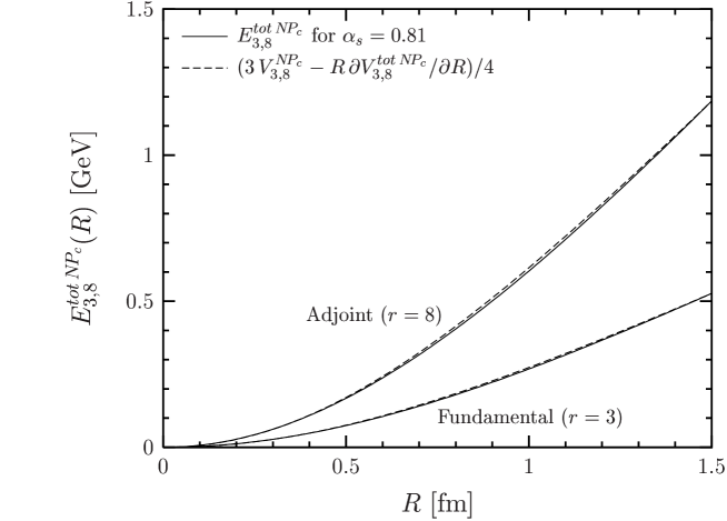
Figure 9: The total energy stored in the chromo-field distributions around a static color dipole of size $R$ in the fundamental ($r=3$) and adjoint ($r=8$) representation of $SU(3)$ from the confining non-perturbative SVM component, $E_{3,8}^{\mbox{\scriptsize tot}\,N\!P_{c}}(R)$, for $\alpha_{s}=0.81$ (solid lines) compared with the relation to the corresponding ground state energy (dashed lines) given by the low-energy theorem (5.4). Good consistency is found even down to very small values of $R$.

we show the total energy stored in the chromo-field distributions around a static color dipole in the fundamental ($r=3$) and adjoint ($r=8$) representation of $SU(3)$ from the confining non-perturbative SVM component, $E_{3,8}^{\mbox{\scriptsize tot}\,N\!P_{c}}(R)$, for $\alpha_{s}=0.81$ (solid lines) as a function of the dipole size $R$. Comparing this total energy, which appears on the LHS of (5.4), with the corresponding RHS of (5.4) (dashed lines), we find good consistency even down to very small values of $R$. This is a nontrivial and important result as it confirms the consistency of our loop-loop correlation result—needed to compute the chromo-electric field—with the result obtained for the VEV of one loop—needed to compute the static potential $V_{r}^{N\!P_{c}}(R)$. Moreover, it shows that the minimal surfaces ensure the consistency of our non-perturbative component. The good consistency found for the pyramid mantle choice of the surface relies on the naively expected energy sum rule [25, 31] in which the contribution from the traceless part of the energy-momentum tensor is not taken into account.

Let us discuss the values of $\beta/g$ and $g^{2}$ at the renormalization scale $\mu_{N\!P}$—given respectively in (5.7) and (5.8)—in comparison with the perturbative expansion [90] and lattice computations [91] of the Callan-Symanzik function in pure $SU(N_{c}=3)$ gauge theory. We obtained (5.7) and (5.8) such that the renormalization scales $\mu_{N\!P}$ appearing in the two equations should be in good agreement. Considering $\beta/g$ as a function $g^{2}$, one thus can compare our combination with the perturbative expansion [90]. This comparison shows that our result is close to the curve obtained on the two-loop level in perturbation theory. In contrast, the non-perturbative lattice results for the $\beta$ function of Lüscher et al. [91] are in good agreement with the perturbative three-loop result computed in the minimal modified subtraction ($\overline{\mathrm{MS}}$) scheme [92]. However, it must be stressed that in the lattice investigation the considered values of the running coupling $g^{2}$ stay below $3.5$ while our comparison requires values up to $g^{2}(\mu_{N\!P})=10.2$. Thus, relying on a large extrapolation of the model independent QCD results, our comparison provides at best an orientation. For a meaningful consistency check, we have to map out the Callan-Symanzik function at smaller values of $R$, where also perturbative correlations must be taken into account and thus refinements of our treatment of renormalization are needed. The low-energy theorems will provide crucial criteria for the success of such improvements.

6 Euclidean Approach to High-Energy Scattering

In this section we present a Euclidean approach to high-energy reactions of color dipoles in the eikonal approximation. After a short review of the functional integral approach to high-energy dipole-dipole scattering in Minkowski space-time, we generalize the analytic continuation introduced by Meggiolaro [35] from parton-parton scattering to dipole-dipole scattering. This shows how one can access high-energy reactions directly in lattice QCD. We apply this approach to compute the scattering of dipoles in the fundamental and adjoint representation of $SU(N_{c})$ at high-energy in the Euclidean LLCM. The result shows the consistency with the analytic continuation of the gluon field strength correlator used in all earlier applications of the SVM and LLCM to high-energy scattering. Finally, we comment on the QCD van der Waals potential which appears in the limiting case of two static color dipoles.

In Minkowski space-time, high-energy reactions of color dipoles in the eikonal approximation have been considered—as basis for hadron-hadron, photon-hadron, and photon-photon reactions—in the functional integral approach to high-energy collisions developed originally for parton-parton scattering [9, 10] and then extended to gauge-invariant dipole-dipole scattering [11, 12, 13]. The corresponding $T$-matrix element for the elastic scattering of two color dipoles at transverse momentum transfer ${\vec{q}}_{\!\perp}$ ($t=-{\vec{q}}_{\!\perp}^{\,\,2}$) and c.m. energy squared $s$ reads

$$T^{M}_{r_{1}r_{2}}(s,t,z_{1},\vec{r}_{1\perp},z_{2},\vec{r}_{2\perp})=2is\int\!\!d^{2}b_{\!\perp}e^{i{\vec{q}}_{\!\perp}{\vec{b}}_{\!\perp}}\left[1-S^{M}_{r_{1}r_{2}}(s,{\vec{b}}_{\!\perp},z_{1},\vec{r}_{1\perp},z_{2},\vec{r}_{2\perp})\right]$$ (6.1)

with the $S$-matrix element ($M$ refers to Minkowski space-time)

$$S^{M}_{r_{1}r_{2}}(s,{\vec{b}}_{\!\perp},z_{1},\vec{r}_{1\perp},z_{2},\vec{r}_{2\perp})=\lim_{T\rightarrow\infty}\frac{\langle W_{r_{1}}[C_{1}]W_{r_{2}}[C_{2}]\rangle_{M}}{\langle W_{r_{1}}[C_{1}]\rangle_{M}\langle W_{r_{2}}[C_{2}]\rangle_{M}}\ .$$ (6.2)

The color dipoles are considered in the $SU(N_{c})$ representation $r_{i}$ and have transverse size and orientation ${\vec{r}}_{i\perp}$. The longitudinal momentum fraction carried by the quark of dipole $i$ is $z_{i}$. [Here and in the following we use several times the term quark generically for color sources in an arbitary $SU(N_{c})$ representation.] The impact parameter between the dipoles is [44]

$${\vec{b}}_{\!\perp}\,=\,{\vec{r}}_{1q}+(1-z_{1}){\vec{r}}_{1\perp}-{\vec{r}}_{2q}-(1-z_{2}){\vec{r}}_{2\perp}\,=\,{\vec{r}}_{1\,cm}-{\vec{r}}_{2\,cm}\ ,$$ (6.3)

where ${\vec{r}}_{iq}$ (${\vec{r}}_{i{\bar{q}}}$) is the transverse position of the quark (antiquark), ${\vec{r}}_{i\perp}={\vec{r}}_{i{\bar{q}}}-{\vec{r}}_{iq}$, and ${\vec{r}}_{i\,cm}=z_{i}{\vec{r}}_{iq}+(1-z_{i}){\vec{r}}_{i{\bar{q}}}$ is the center of light-cone momenta. Figure 10 illustrates the (a) space-time and (b) transverse arrangement of the dipoles.

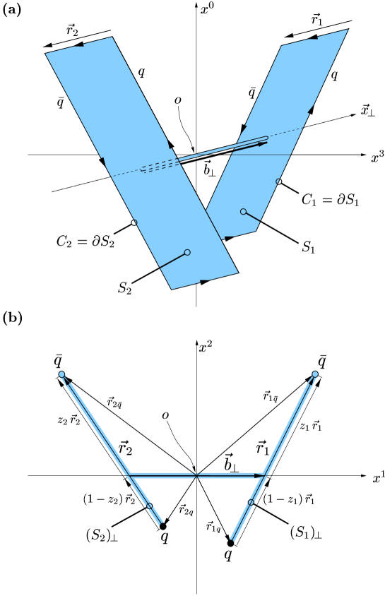
Figure 10: High-energy dipole-dipole scattering in the eikonal approximation represented by Wegner-Wilson loops in the fundamental representation of $SU(N_{c})$: (a) space-time and (b) transverse arrangement of the Wegner-Wilson loops. The shaded areas represent the strings extending from the quark to the antiquark path in each color dipole. The thin tube allows us to compare the field strengths in surface $S_{1}$ with the field strengths in surface $S_{2}$. The impact parameter $\vec{b}_{\perp}$ connects the centers of light-cone momenta of the dipoles.

The dipole trajectories $C_{i}$ are described as straight lines. This is a good approximation as long as the kinematical assumption behind the eikonal approximation, $s\gg-t$, holds which allows us to neglect the change of the dipole velocities $v_{i}=p_{i}/m$ in the scattering process, where $p_{i}$ is the momentum and $m$ the mass of the considered dipole. Moreover, the paths $C_{i}$ are considered light-like in line with the high-energy limit, $m^{2}\ll s\to\infty$. For the hyperbolic angle or rapidity gap between the dipole trajectories $\gamma=(v_{1}\cdot v_{2})$—which is the central quantity in the analytic continuation discussed below and also defined through $s=4m^{2}\cosh^{2}(\gamma/2)$—the high-energy limit implies

$$\lim_{m^{2}\ll s\to\infty}\gamma\approx\ln(s/m^{2})\to\infty\ .$$ (6.4)

The QCD VEV’s $\langle\ldots\rangle_{M}$ in the $S$-matrix element (6.2) represent Minkowskian functional integrals [10] in which—as in the Euclidean case discussed above—the functional integration over the fermion fields has already been carried out.

The Euclidean approach to the described elastic scattering of dipoles in the eikonal approximation is based on Meggiolaro’s analytic continuation of the high-energy parton-parton scattering amplitude [35]. Meggiolaro’s analytic continuation has been derived in the functional integral approach to high-energy collisions [9, 10] in which parton-parton scattering is described in terms of Wegner-Wilson lines: The Minkowskian amplitude, $g^{M}(\gamma,T,t)$, given by the expectation value of two Wegner-Wilson lines, forming a hyperbolic angle $\gamma$ in Minkowski space-time, and the Euclidean “amplitude,” $g^{E}(\Theta,T,t)$, given by the expectation value of two Wegner-Wilson lines, forming an angle $\Theta\in[0,\pi]$ in Euclidean space-time, are connected by the following analytic continuation in the angular variables and the temporal extension $T$, which is needed as an IR regulator in the case of Wegner-Wilson lines,

$$g^{E}(\Theta,T,t) = g^{M}(\gamma\to i\Theta,T\to-iT,t)\ ,$$ (6.5)

$$g^{M}(\gamma,T,t) = g^{E}(\Theta\to-i\gamma,T\to iT,t)\ .$$ (6.6)

Generalizing this relation to gauge-invariant dipole-dipole scattering described in terms of Wegner-Wilson loops, the IR divergence known from the case of Wegner-Wilson lines vanishes and no finite IR regulator $T$ is necessary. Thus, the Minkowskian $S$-matrix element (6.2), given by the expectation values of two Wegner-Wilson loops, forming an hyperbolic angle $\gamma$ in Minkowski space-time, can be computed from the Euclidean “$S$-matrix element”

$$S^{E}_{r_{1}r_{2}}(\Theta,{\vec{b}}_{\!\perp},z_{1},\vec{r}_{1\perp},z_{2},\vec{r}_{2\perp})=\lim_{T\rightarrow\infty}\frac{\langle W_{r_{1}}[C_{1}]W_{r_{2}}[C_{2}]\rangle_{E}}{\langle W_{r_{1}}[C_{1}]\rangle_{E}\langle W_{r_{2}}[C_{2}]\rangle_{E}}$$ (6.7)

given by the expectation values of two Wegner-Wilson loops, forming an angle $\Theta\in[0,\pi]$ in Euclidean space-time, via an analytic continuation in the angular variable

$$S^{M}_{r_{1}r_{2}}(\gamma\approx\ln[s/m^{2}],{\vec{b}}_{\!\perp},z_{1},\vec{r}_{1\perp},z_{2},\vec{r}_{2\perp})=S^{E}_{r_{1}r_{2}}(\Theta\to-i\gamma,{\vec{b}}_{\!\perp},z_{1},\vec{r}_{1\perp},z_{2},\vec{r}_{2\perp})\ ,$$ (6.8)

where $E$ indicates Euclidean space-time and the QCD VEV’s $\langle\ldots\rangle_{E}$ represent Euclidean functional integrals that are equivalent to the ones denoted by $\langle\ldots\rangle_{G}$ in the preceding sections, i.e. in which the functional integration over the fermion fields has already been carried out.

The angle $\Theta$ is best illustrated in the relation of the Euclidean $S$-matrix element (6.7) to the van der Waals potential between two static dipoles, $V_{r_{1}r_{2}}(\Theta=0,\vec{b},z_{1},\vec{r}_{1},z_{2},\vec{r}_{2})$, discussed at the end of this section,

$$S^{E}_{r_{1}r_{2}}(\Theta,\vec{b}_{\!\perp},z_{1},\vec{r}_{1\perp},z_{2},\vec{r}_{2\perp})=\lim_{T\rightarrow\infty}\exp\!\left[-\,T\,V_{r_{1}r_{2}}(\Theta,\vec{b}_{\!\perp},z_{1},\vec{r}_{1\perp},z_{2},\vec{r}_{2\perp})\right]\ .$$ (6.9)

Figure 11 shows the loop-loop geometry necessary to compute $S^{E}_{r_{1}r_{2}}(\Theta\neq 0,\cdots)$ and how it is obtained by generalizing the geometry relevant for the computation of the potential between two static dipoles ($\Theta=0$): While the potential between two static dipoles is computed from two loops along parallel “temporal” unit vectors, $t_{1}=t_{2}=(0,0,0,1)$, the Euclidean $S$-matrix element (6.7) involves the tilting of one of the two loops, e.g. the tilting of $t_{1}$ by the angle $\Theta$ toward the $X_{3}$ axis, $t_{1}=(0,0,-\sin\Theta,\cos\Theta)$. The “temporal” unit vectors $t_{i}$ are also discussed in Appendix B together with another illustration of the tilting angle $\Theta$.

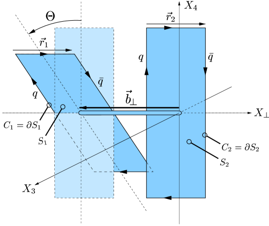
Figure 11: The loop-loop geometry necessary to compute $S^{E}_{r_{1}r_{2}}(\Theta\neq 0,\cdots)$ illustrated as a generalization of the geometry relevant for the computation of the van der Waals potential between two static dipoles ($\Theta=0$). While the potential between two static dipoles is computed from two loops along parallel “temporal” unit vectors, $t_{1}=t_{2}=(0,0,0,1)$, the Euclidean $S$-matrix element (6.7) involves the tilting of one of the two loops, e.g. the tilting of $t_{1}$ by the angle $\Theta$ toward the $X_{3}$ axis, $t_{1}=(0,0,-\sin\Theta,\cos\Theta)$.

Since the Euclidean $S$-matrix element (6.7) involves only configurations of Wegner-Wilson loops in Euclidean space-time and Euclidean functional integrals, it can be computed directly on a Euclidean lattice. With (6.7) evaluated numerically for many different values of $\Theta\in[0,\pi]$, one needs to find the function that describes the angular dependence obtained. If this function is analytic in $\Theta$, the analytic continuation $\Theta\to-i\gamma$ leads immediately to the desired Minkowskian $S$-matrix element (6.2). An obvious difficulty in this proposal is the breaking of rotational invariance by the lattice. Moreover, first attempts in the direction described have shown that the signal size for (6.7) decreases significantly with increasing $\Theta$ so that it is already covered for small values of $\Theta$ by the statistical fluctuations [39]. At present, it is not clear how to overcome these technical difficulties but the stakes are high: Once precise results are available, the analytic continuation (6.8) could allow us to access hadronic high-energy reactions directly in lattice QCD, i.e. within a non-perturbative description of QCD from first principles.

More generally, the presented gauge-invariant analytic continuation (6.8) makes any approach limited to a Euclidean formulation of the theory applicable for investigations of high-energy reactions. Indeed, Meggiolaro’s approach has already been used to access high-energy scattering from the supergravity side of the AdS/CFT correspondence [36], which requires a positive definite metric in the definition of the minimal surface [37], and to examine the effect of instantons on high-energy scattering [38].

Let us now perform the analytic continuation explicitly in our Euclidean model. For the scattering of two color dipoles in the fundamental representation of $SU(N_{c})$, the Euclidean $S$-matrix element becomes with the VEV’s (2.14) and (2.35)

$$S^{E}_{DD}(\Theta,\vec{b}_{\!\perp},z_{1},\vec{r}_{1\perp},z_{2},\vec{r}_{2\perp}) \!\!\!\!\!\!:=\,\,S^{E}_{\mbox{\scriptsize N}_{c}\mbox{\scriptsize N}_{c}}(\Theta,\vec{b}_{\!\perp},z_{1},\vec{r}_{1\perp},z_{2},\vec{r}_{2\perp})$$ (6.10)

$$=\lim_{T\rightarrow\infty}\left(\frac{N_{c}\!+\!1}{2N_{c}}\exp\!\left[-\frac{N_{c}\!-\!1}{2N_{c}}\chi_{S_{1}S_{2}}\right]+\frac{N_{c}\!-\!1}{2N_{c}}\exp\!\left[\frac{N_{c}\!+\!1}{2N_{c}}\chi_{S_{1}S_{2}}\right]\right)\ ,$$

where $\chi_{S_{i}S_{j}}$, defined in (2.27), decomposes into a perturbative ($P$) and non-perturbative ($N\!P$) component according to our decomposition of the gluon field strength correlator (2.42):

$$\chi_{S_{1}S_{2}}\,\,=\,\,\chi_{S_{1}S_{2}}^{P}\,+\,\chi_{S_{1}S_{2}}^{N\!P}\,\,=\,\,\chi_{S_{1}S_{2}}^{P}\,+\,\left(\chi_{S_{1}S_{2}}^{N\!P\,\,nc}\,+\,\chi_{S_{1}S_{2}}^{N\!P\,\,c}\right)\ .$$ (6.11)

In the limit $T_{1}=T_{2}=T\to\infty$ and for $\Theta\in[0,\pi]$, the components read

$$\chi_{S_{1}S_{2}}^{P}=\cot\Theta\,\,\chi^{P}\,\,,\quad\chi_{S_{1}S_{2}}^{N\!P\,\,nc}=\cot\Theta\,\,\chi^{N\!P\,\,nc}\,\,,\quad\chi_{S_{i}S_{j}}^{N\!P\,\,c}=\cot\Theta\,\,\chi^{N\!P\,\,c}$$ (6.12)

with

$$\!\!\!\!\!\!\!\!\!\!\!\!\!\chi^{P} \!\!=\!\! \left[g^{2}D^{\prime\,(2)}_{P}\left(|\vec{r}_{1q}-\vec{r}_{2{\bar{q}}}|\right)+g^{2}D^{\prime\,(2)}_{P}\left(|\vec{r}_{1{\bar{q}}}-\vec{r}_{2q}|\right)\right.$$ (6.13)

$$\left.-\,g^{2}D^{\prime\,(2)}_{P}\left(|\vec{r}_{1q}-\vec{r}_{2q}|\right)-g^{2}D^{\prime\,(2)}_{P}\left(|\vec{r}_{1{\bar{q}}}-\vec{r}_{2{\bar{q}}}|\right)\right]\ ,$$

$$\!\!\!\!\!\!\!\!\!\chi^{N\!P\,\,nc} \!\!=\!\! \frac{\pi^{2}G_{2}(1-\kappa)}{3(N_{c}^{2}-1)}\left[D^{\prime\,(2)}_{1}\left(|\vec{r}_{1q}-\vec{r}_{2{\bar{q}}}|\right)+D^{\prime\,(2)}_{1}\left(|\vec{r}_{1{\bar{q}}}-\vec{r}_{2q}|\right)\right.$$ (6.14)

$$\hphantom{-\frac{\pi^{2}G_{2}(1-\kappa)}{3(N_{c}^{2}-1)}}\left.-\,D^{\prime\,(2)}_{1}\left(|\vec{r}_{1q}-\vec{r}_{2q}|\right)-D^{\prime\,(2)}_{1}\left(|\vec{r}_{1{\bar{q}}}-\vec{r}_{2{\bar{q}}}|\right)\right]\ ,$$

$$\!\!\!\!\!\!\!\!\!\!\!\!\!\chi^{N\!P\,\,c} \!\!=\!\! \frac{\pi^{2}G_{2}\kappa}{3(N_{c}^{2}-1)}\,\left(\vec{r}_{1}\cdot\vec{r}_{2}\right)\int_{0}^{1}\!dv_{1}\int_{0}^{1}\!dv_{2}\,\,D^{(2)}\left(|\vec{r}_{1q}\!+\!v_{1}\vec{r}_{1\perp}\!-\!\vec{r}_{2q}\!-\!v_{2}\vec{r}_{2\perp}|\right)$$ (6.15)

as derived explicitly in Appendix C with the minimal surfaces illustrated in Fig. 11. In Eq. (6.13) the shorthand notation $g^{2}D^{\prime\,(2)}_{P}(|\vec{Z_{\perp}}|)=g^{2}(|\vec{Z_{\perp}}|)\,D^{\prime\,(2)}_{P}(|\vec{Z_{\perp}}|)$ is used with $g^{2}(|\vec{Z_{\perp}}|)$ again understood as the running coupling (2.47). The transverse Euclidean correlation functions

$$D_{x}^{(2)}(\vec{Z}^{2}):=\int\frac{d^{4}K}{(2\pi)^{2}}\,e^{iKZ}\,\tilde{D}_{x}(K^{2})\,\delta(K_{3})\,\delta(K_{4})$$ (6.16)

are obtained from the (massive) gluon propagator (2.43) and the exponential correlation function (2.50)

$$\!\!\!\!\!\!\!\!\!\!\!\!\!\!\!\!D^{\prime\,(2)}_{P}(\vec{Z}_{\!\perp}^{2}) \!\!=\!\! \frac{1}{2\pi}K_{0}\left(m_{G}|\vec{Z}_{\!\perp}|\right)$$ (6.17)

$$\!\!\!\!\!\!\!\!\!\!\!\!\!\!\!\!D^{\prime\,(2)}_{1}(\vec{Z}_{\!\perp}^{2}) \!\!=\!\! \pi a^{4}\Big{(}3\!+\!3\frac{|\vec{Z}_{\!\perp}|}{a}\!+\!\frac{|\vec{Z}_{\!\perp}|^{2}}{a^{2}}\Big{)}\exp\!\Big{(}\!-\frac{|\vec{Z}_{\!\perp}|}{a}\Big{)}$$ (6.18)

$$\!\!\!\!\!\!\!\!\!\!\!\!\!\!\!\!D^{(2)}(\vec{Z}_{\!\perp}^{2}) \!\!=\!\! 2\pi a^{2}\Big{(}1\!+\!\frac{|\vec{Z}_{\!\perp}|}{a}\Big{)}\exp\!\Big{(}\!-\frac{|\vec{Z}_{\!\perp}|}{a}\Big{)}$$ (6.19)

With the full $\Theta$ dependence exposed in (6.12), the analytic continuation (6.8) reads

$$\chi_{S_{1}S_{2}}=\cot\Theta\,\,\chi\quad\underrightarrow{\,\,\Theta\to-i\gamma\,\,\,\,}\quad\cot(-i\gamma)\,\chi\quad\underrightarrow{\,\,s\to\infty\,\,\,\,}\quad i\chi$$ (6.20)

and leads to the desired Minkowskian $S$-matrix element for elastic dipole-dipole ($DD$) scattering in the high-energy limit in which the dipoles move on the light cone:

$$\lim_{s\rightarrow\infty}S_{DD}^{M}(s,{\vec{b}}_{\!\perp},z_{1},\vec{r}_{1\perp},z_{2},\vec{r}_{2\perp}) \!\!\!\!\!\!:=\,\,\lim_{s\rightarrow\infty}S^{M}_{\mbox{\scriptsize N}_{c}\mbox{\scriptsize N}_{c}}(s,{\vec{b}}_{\!\perp},z_{1},\vec{r}_{1\perp},z_{2},\vec{r}_{2\perp})$$ (6.21)

$$=S^{E}_{DD}(\cot\Theta\to i,{\vec{b}}_{\!\perp},z_{1},\vec{r}_{1\perp},z_{2},\vec{r}_{2\perp})$$

$$=\lim_{T\rightarrow\infty}\left(\frac{N_{c}\!+\!1}{2N_{c}}\exp\!\left[-i\frac{N_{c}\!-\!1}{2N_{c}}\chi\right]+\frac{N_{c}\!-\!1}{2N_{c}}\exp\!\left[i\frac{N_{c}\!+\!1}{2N_{c}}\chi\right]\right),$$

where $\chi=\chi^{P}+\chi^{N\!P\,\,nc}+\chi^{N\!P\,\,c}$ with (6.13), (6.14), and (6.15).

It is striking that exactly the same result was obtained in [8] with the alternative analytic continuation introduced for applications of the SVM to high-energy reactions [11, 12, 13]. In this complementary approach the gauge-invariant bilocal gluon field strength correlator is analytically continued from Euclidean to Minkowskian space-time by the substitution $\delta_{\mu\rho}\rightarrow-g_{\mu\rho}$ and the analytic continuation of the Euclidean correlation functions to real time $D^{E}_{x}(Z^{2})\rightarrow D^{M}_{x}(z^{2})$. In the subsequent steps, one finds $\langle W[C]\rangle_{M}=1$ due to the light-likeness of the loops and that the longitudinal correlations can be integrated out $\langle W_{r_{1}}[C_{1}]W_{r_{2}}[C_{2}]\rangle_{M}=f(s,{\vec{b}}_{\!\perp},\cdots)$. One is left with exactly the Euclidean correlations in transverse space that have been obtained above. This confirms the analytic continuation used in the earlier LLCM investigations in Minkowski space-time [8, 32, 33, 34] and in all earlier SVM applications to high-energy scattering [11, 12, 13, 40, 41, 42, 43, 44, 45, 48, 46, 47].

In the limit of small $\chi$ functions, $|\chi^{P}|\ll 1$ and $|\chi^{N\!P}|\ll 1$, Eq. (6.21) reduces to

$$\lim_{s\rightarrow\infty}S_{DD}^{M}(s,{\vec{b}}_{\!\perp},z_{1},\vec{r}_{1\perp},z_{2},\vec{r}_{2\perp})\approx 1+\frac{N_{c}^{2}-1}{8N_{c}^{2}}\,\chi^{2}=1+\frac{C_{2}(\mbox{N}_{c})}{4N_{c}}\,\chi^{2}\ .$$ (6.22)

The perturbative correlations, $(\chi^{P})^{2}$, describe the well-known two-gluon exchange contribution [93, 94] to dipole-dipole scattering, which is, of course, an important successful cross-check of the presented Euclidean approach to high-energy scattering. The non-perturbative correlations, $(\chi^{N\!P})^{2}$, describe the corresponding non-perturbative two-point interactions that contain contributions of the confining QCD string to dipole-dipole scattering. We analyzed these string contributions systematically as manifestations of confinement in high-energy scattering reactions in our previous work [33].

From the small-$\chi$ limit, one sees that the full $S$-matrix element (6.21) describes multiple gluonic interactions. Indeed, the higher order terms in the expansion of the exponential functions ensure the fundamental $S$-matrix unitarity condition in impact parameter space as discussed in [45, 8].

Concerning the energy dependence, the $S$-matrix element (6.21) leads to energy-independent cross sections in contradiction to the experimental observation. Although disappointing from the phenomenological point of view, this is not surprising since our approach does not describe the explicit gluon radiation needed for a non-trivial energy dependence. However, based on the $S$-matrix element (6.21), a phenomenological energy dependence can be constructed that allows a unified description of high-energy hadron-hadron, photon-hadron, and photon-photon reactions and an investigation of saturation effects in hadronic cross sections manifesting the $S$-matrix unitarity [8, 32, 34]. This, of course, can only be an intermediate step. For a more fundamental understanding of hadronic high-energy reactions in our model, gluon radiation and quantum evolution have to be implemented explicitly.

Although the scattering of two color dipoles in the fundamental representation of $SU(N_{c})$ is, of course, the most relevant case, we can derive immediately also the Minkowskian $S$-matrix element for the scattering of a fundamental ($D$) and an adjoint dipole (“glueball” $G\!B$) in the Euclidean LLCM. Using (2.40) and proceeding otherwise as above, we find in the high-energy limit

$$\!\!\!\!\!\!\!\!\lim_{s\rightarrow\infty}S^{M}_{D\,G\!B}(s,\vec{b},z_{1},\vec{r}_{1},z_{2},\vec{r}_{2})\,\,:=\,\,\lim_{s\rightarrow\infty}S^{M}_{\mbox{\scriptsize N}_{c}\,\mbox{\scriptsize N}_{c}^{2}\!-\!1}(\Theta,\vec{b},z_{1},\vec{r}_{1},z_{2},\vec{r}_{2})$$ (6.23)

$$\!\!\!\!\!\!\!\!=\lim_{T\rightarrow\infty}\Bigg{(}\,\frac{1}{N_{c}^{2}\!-\!1}\,\exp\!\Big{[}i\,\frac{N_{c}}{2}\,\chi\Big{]}+\frac{N_{c}\!+\!2}{2(N_{c}\!+\!1)}\exp\!\Big{[}\!-\,i\,\frac{1}{2}\,\chi\Big{]}+\frac{N_{c}\!-\!2}{2(N_{c}\!-\!1)}\exp\!\Big{[}i\,\frac{1}{2}\,\chi\Big{]}\Bigg{)}\ ,$$

where $\chi=\chi^{P}+\chi^{N\!P\,nc}+\chi^{N\!P\,c}$ with (6.13), (6.14), and (6.15).

Finally, we would like to comment on the van der Waals interaction of two color dipoles, which is, as already mentioned, related to the Euclidean $S$-matrix element in the limiting case of $\Theta=0$ as can be seen from (6.9): The QCD van der Waals potential between two static dipoles can be expressed in terms of Wegner-Wilson loops [95, 96]

$$V_{r_{1}r_{2}}(\Theta=0,\vec{b},z_{1}=1/2,\vec{r}_{1},z_{2}=1/2,\vec{r}_{2})=-\lim_{T\rightarrow\infty}\frac{1}{T}\ln\frac{\langle W_{r_{1}}[C_{1}]W_{r_{2}}[C_{2}]\rangle}{\langle W_{r_{1}}[C_{1}]\rangle\langle W_{r_{2}}[C_{2}]\rangle}\ .$$ (6.24)

In this limit ($\Theta=0$) intermediate octet states and their limited lifetime become important as is well known from perturbative computations of the QCD van der Waals potential between two static color dipoles [95, 96, 97]: Working with static dipoles, i.e. infinitely heavy color sources, there is an energy degeneracy between the intermediate octet states and the initial (final) singlet states that leads for perturbative two-gluon exchange to a linear divergence in $T$ as $T\to\infty$. This IR divergence can be lifted by manually introducing an energy gap between the singlet ground state and the excited octet state and thus a limit on the lifetime of the intermediate octet state [95, 96, 97].

In the perturbative limit of $g^{2}\to 0$ and $T$ large but finite, i.e. $\chi^{P}\ll 1$, the perturbative component of our model describes the two-gluon exchange contribution to the van der Waals potential which is plagued by this IR divergence due to the static limit. In the more general case of $g^{2}$ finite and $T\to\infty$, which is applicable also for the non-perturbative component of our model, one cannot use the small-$\chi$ limit and multiple gluonic interactions become important. Here, our perturbative component describes multiple gluon exchanges that reduce to an effective one-gluon exchange contribution to the van der Waals potential whose interaction range ($\propto 1/m_{G}$) contradicts the common expectations. Indeed, it is also in contradiction to our results for the glueball mass $M_{G\!B}$ which determines the interaction range ($\propto 1/M_{G\!B}$) between two color dipoles for large dipole separations. As already mentioned in Sec. 2.3, we find for the perturbative component, $M_{G\!B}^{P}=2m_{G}$, i.e. half of the interaction range of one-gluon exchange, by computing the exponential decay of the correlation of two small quadratic loops $P^{\alpha\beta}_{r_{i}}$ for large Euclidean times $\tau\to\infty$,

$$M_{G\!B}:=-\lim_{\tau\rightarrow\infty}\frac{1}{\tau}\ln\frac{\langle P_{r_{1}}^{\alpha\beta}(0)P_{r_{2}}^{\alpha\beta}(\tau)\rangle}{\langle P_{r_{1}}^{\alpha\beta}(0)\rangle\langle P_{r_{2}}^{\alpha\beta}(\tau)\rangle}\ .$$ (6.25)

Note that we find for the non-perturbative component, $M_{G\!B}^{N\!P}=2/a$, which is smaller than $M_{G\!B}^{P}=2m_{G}$ with the LLCM parameters and thus governs the long range correlations in the LLCM.

Thus, for a meaningful investigation of the QCD van der Waals forces within our model, one has to go beyond the static limit in order to describe the limited lifetime of the intermediate octet states appropriately. This we postpone for future work since the focus in this work is on high-energy scattering where the gluons are always exchanged within a short time interval due to the light-likeness of the scattered particles and the finite correlation lengths. Nevertheless, going beyond the static limit in the dipole-dipole potential means going beyond the eikonal approximation in high-energy scattering and it is, of course, of utmost importance to see how such generalizations alter our results.

7 Conclusion

We have introduced the Euclidean version of the loop-loop correlation model [8] in which the QCD vacuum is described by perturbative gluon exchange and the non-perturbative stochastic vacuum model [21]. This combination leads to a static quark-antiquark potential with color Coulomb behavior for small and confining linear rise for large source separations in good agreement with lattice QCD results. We have computed in the LLCM the vacuum expectation value of one Wegner-Wilson loop, $\langle W_{r}[C]\rangle$, and the correlation of two Wegner-Wilson loops, $\langle W_{r_{1}}[C_{1}]W_{r_{2}}[C_{2}]\rangle$, for arbitrary loop geometries and general representations $r_{(i)}$ of $SU(N_{c})$. Specifying the loop geometries, these results allow us to compute the static quark-antiquark potential, the glueball mass, the chromo-field distributions of static color dipoles, the QCD van der Waals potential between two static color dipoles, and the $S$-matrix element for high-energy dipole-dipole scattering.

We have applied the LLCM to compute the potential and the chromo-electric fields of a static color dipole in the fundamental and adjoint representation of $SU(N_{c})$. The formation of a confining color flux tube is described by the non-perturbative SVM correlations [25] and the color Coulomb field is obtained from perturbative gluon exchange. We have found Casimir scaling for both the perturbative and non-perturbative contributions to the chromo-electric fields in agreement with recent lattice data [20]. String breaking is described neither for sources in the fundamental representation nor for sources in the adjoint representation, which indicates that in our approach not only dynamical fermions (quenched approximation) are missing but also some gluon dynamics. Transverse and longitudinal energy density profiles have been provided. For small dipoles, $R=0.1\,\mbox{fm}$, perturbative physics dominates and non-perturbative correlations are negligible. For large dipoles, $R\gtrsim 1\,\mbox{fm}$, the non-perturbative confining string dominates the chromo-electric fields between the color sources. The transition from perturbative to string behavior takes place at source separations of about $0.5\,\mbox{fm}$ in agreement with the recent results of Lüscher and Weisz [26]. The root mean squared radius $R_{ms}$ of the confining string and the energy density in the center of a fundamental $SU(3)$ dipole $\varepsilon_{3}(X=0)$ are governed completely by non-perturbative physics for large $R$ and saturate as $R$ increases at $R_{ms}^{R\to\infty}\approx 0.55\,\mbox{fm}$ and $\varepsilon_{3}^{R\to\infty}(X=0)\approx 1\,\mbox{GeV}/\mbox{fm}^{3}$.

We have presented the low-energy theorems [28, 29, 30], known in lattice QCD as Michael sum rules [27], in their complete form in continuum theory taking into account the important contributions found in [31, 28] that are missing in the original formulation [27]. We have used the complete theorems to compare the energy and action stored in the confining string with the confining part of the static quark-antiquark potential. The comparison shows consistency of the model results and indicates that the non-perturbative SVM component is working at the renormalization scale at which $\beta(g)/g=-2$ and $\alpha_{s}=0.81$. Earlier SVM investigations along these lines have found a different value of $\alpha_{s}=0.57$ with the pyramid mantle choice for the surface [25, 31] but were incomplete since only the contribution from the traceless part of the energy-momentum tensor has been considered in the energy sum.

A Euclidean approach to high-energy dipole-dipole scattering has been established by generalizing Meggiolaro’s analytic continuation [35] from parton-parton scattering to gauge-invariant dipole-dipole scattering. The generalized analytic continuation allows us to derive $S$-matrix elements for high-energy reactions from configurations of Wegner-Wilson loops in Euclidean space-time with Euclidean functional integrals. It thus shows how one can access high-energy reactions directly in lattice QCD. First attempts in this direction have already been carried out but only very few signals could be extracted, while most of the data were dominated by noise [39]. We have applied this approach to compute in the Euclidean LLCM the scattering of dipoles at high-energy. The result derived in the Minkowskian version of the LLCM [8] has been exactly recovered including the well-known two-gluon exchange contribution to dipole-dipole scattering [93, 94]. This confirms the analytic continuation of the gluon field strength correlator used in all earlier applications of the SVM to high-energy scattering [11, 12, 13, 40, 41, 42, 43, 44, 45, 48, 46, 47].

The $S$-matrix element obtained in our approach has already been used to investigate manifestations of the confining QCD string in high-energy reactions of photons and hadrons [33] but leads to energy-independent cross sections in contradiction to the experimental observation [8]. The missing energy dependence is disappointing but not surprising since our approach does not describe explicit gluon radiation needed for a non-trivial energy dependence. In our previous work we have introduced a phenomenological energy dependence into the $S$-matrix element that allows a unified description of hadron-hadron, photon-hadron, and photon-photon reactions and respects the $S$-matrix unitarity condition in impact parameter space [8, 32, 34]. However, for a more fundamental understanding of hadronic high-energy reactions in our model, one faces the highly ambitious task to implement gluon radiation and quantum evolution explicitly.

More generally, the presented Euclidean approach to high-energy scattering makes any method limited to a Euclidean formulation of the theory applicable for investigations of high-energy reactions. Here encouraging new results have been obtained with instantons [38] and within the AdS/CFT correspondence [36] and it will be interesting to see precise results from the lattice. A promising complementary Euclidean approach has been proposed in [98] where the structure functions of deep inelastic scattering at small Bjorken $x$ are related to an effective Euclidean field theory. Here one hopes that the limit $x\to 0$ corresponds to critical behavior in the effective theory. The aim is again to provide a framework in which structure functions can be calculated from first principles using genuine non-perturbative methods such as lattice computations. In another recent attempt, the energy dependence of the proton structure function has been related successfully to critical properties of an effective near light-cone Hamiltonian in a non-perturbative lattice approach [99]. It will be interesting to see further developments along these lines aiming at an understanding of hadronic high-energy scattering from the QCD Lagrangian.

Appendix A The non-Abelian Stokes Theorem

In this appendix we review briefly the derivation of the non-Abelian Stokes theorem [16] and explain the emerging surface ordering. We follow the lucid presentation given in [10].

Let us consider a surface $S$ in Euclidean space-time with boundary $C=\partial S$ and the QCD Schwinger string $\Phi_{r}(X,X;C)$ defined according to (2.5) that starts at some point $X$ on the boundary and evolves along the path $C$ back to the point $X$ as illustrated in Fig. 12. We now explain how the non-Abelian line integral over $C$ associated with the QCD Schwinger string is transformed into the non-Abelian surface integral over $S$ which involves the surface ordering ${\cal P}_{S}$.

Figure 12: A surface $S$ with boundary $C=\partial S$ in Euclidean space-time, the reference point $O$ on $S$, and the fan-type net with center $O$ spanned over $S$.

First, we choose an arbitrary reference point $O$ on the surface $S$ and draw a fan-type net on $S$ as a spider could do (cf. Fig. 12). This net is spanned over $S$ and is given by the following curve: $C_{XO}$ running from $X$ to $O$, followed by $C_{Z_{1}O}^{-1}$ running from $O$ to $Z_{1}$, where the path around the infinitesimal small square $\Delta\sigma_{\mu\nu}(Z_{1})$, i.e. the plaquette at $Z_{1}$, is attached before it goes back to $O$ along $C_{Z_{1}O}$ and so on. The net is completed with $C_{XO}^{-1}$ that runs from $O$ to $X$. Apart from the initial and final elements of the net, $C_{XO}$ and $C_{XO}^{-1}$, we have many plaquettes with “handles” connecting them to $O$. With the following basic properties of the QCD Schwinger string,

$$\Phi_{r}(O,X;C_{XO})\,\Phi_{r}(O,X;C_{XO})^{-1} = {1\!\rm l}\ ,$$ (A.1)

$$\Phi_{r}(O,X;C_{XO})^{-1}\,\,=\,\,\,\Phi_{r}^{\dagger}(O,X;C_{XO}) = \Phi_{r}(X,O;C_{OX}=C^{-1}_{XO})\ ,$$ (A.2)

$$\Phi_{r}(Z,X;C_{XZ})\,\Phi_{r}(X,O;C_{OX}) = \Phi_{r}(Z,O;C_{OX}+C_{XZ})\ ,$$ (A.3)

one sees immediately that the QCD Schwinger string along the net spanned on $S$ is equivalent to the QCD Schwinger string $\Phi_{r}(X,X;C)$ along the path $C$:

$$\Phi_{r}(X,X;C) = \Phi_{r}(O,X;C_{XO})\cdot\big{(}\mbox{product of QCD Schwinger strings}$$ (A.4)

$$\mbox{for the plaquettes with handles}\big{)}\cdot\Phi_{r}(O,X;C_{XO})^{-1}\ .$$

Next, we consider the contribution of a single plaquette with handle. The QCD Schwinger string for one plaquette, say the one at $Z_{n}$ singled out in Fig. 12, reads [10]

$$\Phi_{r}(\mbox{plaquette at $Z_{n}$})={1\!\rm l}-ig\frac{1}{2}\Delta\sigma_{\mu\nu}(Z_{n})\,{\cal G}^{a}_{\mu\nu}(Z_{n})\,t_{r}^{a}+\,\cdots\,\ .$$ (A.5)

where $\Delta\sigma_{\mu\nu}(Z_{n})$ denotes the surface element at the point $Z_{n}$. Taking into account the handles, the contribution of this plaquette to (A.4) becomes

$$\Phi_{r}(O,Z_{n};C_{Z_{n}O})\Phi_{r}(\mbox{plaquette at $Z_{n}$})\Phi_{r}(O,Z_{n};C_{Z_{n}O})^{-1}$$

$$={1\!\rm l}-ig\frac{1}{2}\Delta\sigma_{\mu\nu}(Z_{n})\,{\cal G}^{a}_{\mu\nu}(O,Z_{n};C_{Z_{n}O})\,t_{r}^{a}+\,\cdots\,\ ,$$ (A.6)

where (A.2) and the parallel transported gluon field strength as defined in (2.4) have been used.

Finally, inserting (A.6) into (A.4) for all $n$, i.e. summing up the contributions of all plaquettes with handles, while respecting the ordering, one obtains in the limit of an infinitesimally fine net

$$\Phi_{r}(X,X;C)=\Phi_{r}(O,X;C_{XO})$$ (A.7)

$$\quad\quad\quad\quad\cdot\,{\cal P}_{S}\exp\left[-i\,\frac{g}{2}\int_{S}\!d\sigma_{\mu\nu}(Z){\cal G}^{a}_{\mu\nu}(O,Z;C_{ZO})\,t_{r}^{a}\right]\cdot\Phi_{r}(O,X;C_{XO})^{-1}\ .$$

Here ${\cal P}_{S}$ denotes the ordering on the whole surface $S$ as implied by the net shown in Fig. 12. Taking the trace in (A.7) and exploiting its cyclic property leads ultimately to the non-Abelian version of Stokes theorem

$$\mbox{Tr}_{r}\,\Phi_{r}(X,X;C)=\mbox{Tr}_{r}\,{\cal P}_{S}\exp\left[-i\,\frac{g}{2}\int_{S}\!d\sigma_{\mu\nu}(Z){\cal G}^{a}_{\mu\nu}(O,Z;C_{ZO})\,t_{r}^{a}\right]\ .$$ (A.8)

Appendix B Loop and Minimal Surface Parametrizations

A rectangular loop $C_{i}$ with “spatial” extension $R_{i}$ and “temporal” extension $2T_{i}$ placed in four-dimensional Euclidean space, as shown in Fig. 13, has the following parameter representation:

$$C_{i}\,\,=\,\,C_{i}^{A}\,\cup\,C_{i}^{B}\,\cup\,C_{i}^{C}\,\cup\,C_{i}^{D}$$ (B.1)

with

$$C_{i}^{A}\,\,=\,\,\Big{\{}X_{i}^{A}(u_{i}) = X_{\!0\,i}-(1-z_{i})\,r_{i}+u_{i}\,t_{i},\quad\hphantom{v_{i}\,r_{i}}u_{i}\in[-T_{i},T_{i}]\Big{\}}$$ (B.2)

$$C_{i}^{B}\,\,=\,\,\Big{\{}X_{i}^{B}(v_{i}) = X_{\!0\,i}-(1-z_{i})\,r_{i}+v_{i}\,r_{i}+T_{i}\,t_{i},\;\quad v_{i}\in[0,1]\Big{\}}$$ (B.3)

$$C_{i}^{C}\,\,=\,\,\Big{\{}X_{i}^{C}(u_{i}) = X_{\!0\,i}+z_{i}\,r_{i}+u_{i}\,t_{i},\quad\hphantom{(1-z_{i})\,r_{i}}u_{i}\in[T_{i},-T_{i}]\Big{\}}$$ (B.4)

$$C_{i}^{D}\,\,=\,\,\Big{\{}X_{i}^{D}(v_{i}) = X_{\!0\,i}-(1-z_{i})\,r_{i}+v_{i}\,r_{i}-T_{i}\,t_{i},\;\quad v_{i}\in[1,0]\Big{\}}$$ (B.5)

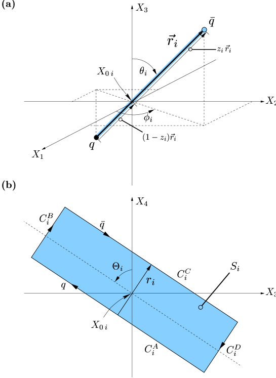
Figure 13: (a) Spatial arrangement of a color dipole and (b) its world-line in Euclidean “longitudinal” space given by the rectangular loop $C_{i}$ that defines the minimal surface $S_{i}$ with $\partial S_{i}=C_{i}$. The minimal surface is represented by the shaded area. In our model, it is interpreted as the world-sheet of the QCD string that confines the quark and antiquark in the dipole.

where

$$r_{i}:=\left(\begin{array}[]{c}R_{i}\,\sin\theta_{i}\,\cos\phi_{i}\\ R_{i}\,\sin\theta_{i}\,\sin\phi_{i}\\ R_{i}\,\cos\theta_{i}\,\cos\Theta_{i}\\ R_{i}\,\cos\theta_{i}\,\sin\Theta_{i}\end{array}\right)\quad\mbox{and}\quad t_{i}:=\left(\!\!\begin{array}[]{c}0\\ 0\\ -\sin\Theta_{i}\\ \hphantom{-}\cos\Theta_{i}\end{array}\right)\ .$$ (B.6)

The “center” of the loop $C_{i}$ is given by $X_{\!0\,i}$. The parameters $z_{i}$, $R_{i}$, $\theta_{i}$, $\phi_{i}$, and $\Theta_{i}$ are defined in Fig. 13 which illustrates (a) the spatial arrangement of a color dipole and (b) its world-line $C_{i}$ in Euclidean “longitudinal” space. The tilting angle $\Theta_{i}\neq 0$ is the central quantity in the analytic continuation presented in Sec. 6. Moreover, $\Theta_{1}=\pi/2$ together with $\Theta_{2}=0$ allows us to compute conveniently the chromo-magnetic field distributions in Appendix C.

The minimal surface $S_{i}$ is the planar surface bounded by the loop $C_{i}=\partial S_{i}$ given in (B.1). It can be parametrized as follows

$$S_{i}=\Big{\{}X_{i}(u_{i},v_{i})=X_{\!0\,i}-(1-z_{i})\,r_{i}+v_{i}\,r_{i}+u_{i}\,t_{i},\;u_{i}\in[-T_{i},T_{i}],\;v_{i}\in[0,1]\Big{\}}$$ (B.7)

with $r_{i}$ and $t_{i}$ given in (B.6). The corresponding infinitesimal surface element reads

$$d\sigma_{\mu\nu}(X_{i})=\Bigg{(}\frac{\partial X_{\!i\mu}}{\partial u_{i}}\frac{\partial X_{\!i\nu}}{\partial v_{i}}-\frac{\partial X_{\!i\mu}}{\partial v_{i}}\frac{\partial X_{\!i\nu}}{\partial u_{i}}\Bigg{)}\,du_{i}\,dv_{i}=\Bigg{(}t_{i\mu}r_{i\nu}-r_{i\mu}t_{i\nu}\Bigg{)}\,du_{i}\,dv_{i}\ .$$ (B.8)

Appendix C $\chi$ Computations with Minimal Surfaces

The quantities considered in the main text are computed from the VEV of one loop $\langle W[C]\rangle$ and the loop-loop correlation function $\langle W[C_{1}]W[C_{2}]\rangle$. Using the Gaussian approximation in the gluon field strengths, both are expressed in terms of $\chi_{S_{i}S_{j}}$ functions (2.15) and (2.27) as shown in Secs. 2.1 and 2.2. These $\chi$ functions are central quantities since here the ansatz of the gauge-invariant bilocal gluon field strength correlator and the surface choice enter the model. In this appendix, these functions are computed explicitly for minimal surfaces (B.7) and the $F_{\mu\nu\rho\sigma}$ ansatz given in (2.42), (2.3), and (2.3). Note that the contributions from the infinitesimally thin tube—which allows us to compare the field strengths in surface $S_{1}$ with the field strength in surface $S_{2}$—cancel mutually.

Depending on the geometries and the relative arrangement of the loops, the $\chi$ functions determine the physical quantities investigated within the LLCM such as the static $q{\bar{q}}$ potential (3.2), the chromo-field distributions of a color dipole (4.9), and the $S$-matrix element for elastic dipole-dipole scattering (6.10).

We compute the three components $\chi_{S_{1}S_{2}}^{P}$, $\chi_{S_{1}S_{2}}^{N\!P\,nc}$, and $\chi_{S_{1}S_{2}}^{N\!P\,c}$ separately for general loop arrangements from which the considered quantities are obtained as special cases. Without loss of generality, the center of the loop $C_{2}$ is placed at the origin of the coordinate system, $X_{\!0\,2}=(0,0,0,0)$. Moreover, $C_{2}$ is kept untilted, $\Theta_{2}=0$, and $\Theta:=\Theta_{1}$ is used to simplify notation. We limit our general computation to loops with $r_{1,2}=(\vec{r}_{1,2\perp},0,0)\,\,\equiv\,\,\theta_{1,2}=\pi/2$ and transverse “impact parameters” $b=X_{\!0\,1}-X_{\!0\,2}=X_{\!0\,1}=(b_{1},b_{2},0,0)=(\vec{b}_{\!\perp},0,0)$ which allows us to compute all of the considered quantities.

$\chi_{S_{1}S_{2}}^{N\!P\,c}$ Computation

Starting with the definition

$$\chi_{S_{1}S_{2}}^{N\!P\,c} := \frac{\pi^{2}}{4}\int_{S_{1}}\!\!d\sigma_{\mu\nu}(X_{1})\int_{S_{2}}\!\!d\sigma_{\rho\sigma}(X_{2})\,F_{\mu\nu\rho\sigma}^{N\!P\,c}(Z=X_{1}-X_{2})$$

$$= \frac{\pi^{2}G_{2}\kappa}{12(N_{c}^{2}-1)}\int_{S_{1}}\!\!d\sigma_{\mu\nu}(X_{1})\int_{S_{2}}\!\!d\sigma_{\rho\sigma}(X_{2})\left(\delta_{\mu\rho}\delta_{\nu\sigma}-\delta_{\mu\sigma}\delta_{\nu\rho}\right)D(Z^{2})\ ,$$

one exploits the anti-symmetry of the surface elements, $d\sigma_{\mu\nu}=-d\sigma_{\nu\mu}$, and applies the surface parametrization (B.7) with the corresponding surface elements (B.8) to obtain

$$\chi_{S_{1}S_{2}}^{N\!P\,c}=\cos\Theta\,\frac{\pi^{2}G_{2}\kappa}{3(N_{c}^{2}-1)}\,(r_{1}\cdot r_{2})\int_{0}^{1}\!\!dv_{1}\int_{0}^{1}\!\!dv_{2}\int_{-T_{1}}^{T_{1}}\!\!du_{1}\int_{-T_{2}}^{T_{2}}\!\!du_{2}\,D(Z^{2})$$ (C.2)

with

$$Z=X_{1}-X_{2}=\left(\begin{array}[]{l}\!\!\hphantom{-\,}\vec{b}_{\!\perp}-(1-z_{1})\,\vec{r}_{1\perp}+v_{1}\,\vec{r}_{1\perp}+(1-z_{2})\,\vec{r}_{2\perp}-v_{2}\,\vec{r}_{2\perp}\\ \!\!-\,u_{1}\sin\Theta\\ \!\!\hphantom{-\,}u_{1}\cos\Theta-u_{2}\end{array}\right)\ ,$$ (C.3)

where the identities $t_{1}\cdot r_{2}=r_{1}\cdot t_{2}=0$ and $t_{1}\cdot t_{2}=\cos\Theta$, evident from (B.6) with the mentioned specification of the loop geometries, have been used. In the limit $T_{2}\rightarrow\infty$, the $u_{2}$ integration can be performed

$$\lim_{T_{2}\to\infty}\int_{-T_{2}}^{T_{2}}\!\!du_{2}\,D(Z^{2})\,\,=\,\,\int\frac{d^{4}K}{(2\pi)^{4}}\,\tilde{D}(K^{2})\lim_{T_{2}\to\infty}\int_{-T_{2}}^{T_{2}}\!\!du_{2}\,e^{iKZ}$$

$$=\int\frac{d^{4}K}{(2\pi)^{4}}\,\tilde{D}(K^{2})\,2\pi\,\delta(K_{4})\,\exp\!\left[i\vec{K}_{\!\perp}\vec{Z}_{\!\perp}+iK_{3}u_{1}\sin\Theta+iK_{4}u_{1}\cos\Theta\right]$$

$$=\int\frac{d^{3}K}{(2\pi)^{3}}\,\tilde{D}^{(3)}(\vec{K}^{2})\,\exp\!\left[i\vec{K}_{\!\perp}\vec{Z}_{\!\perp}+iK_{3}u_{1}\sin\Theta\right]\,\,=\,\,D^{(3)}(\vec{Z}^{2})\ ,$$ (C.4)

which leads to

$$\lim_{T_{2}\to\infty}\chi_{S_{1}S_{2}}^{N\!P\,c}=\cos\Theta\,\frac{\pi^{2}G_{2}\kappa}{3(N_{c}^{2}-1)}\,(\vec{r}_{1\perp}\cdot\vec{r}_{2\perp})\int_{0}^{1}\!\!dv_{1}\int_{0}^{1}\!\!dv_{2}\int_{-T_{1}}^{T_{1}}\!\!du_{1}\,D^{(3)}(\vec{Z}^{2})\ .$$ (C.5)

Taking in addition the limit $T_{1}\rightarrow\infty$, the $u_{1}$ integration can be performed as well

$$\lim_{T_{1}\to\infty}\int_{-T_{1}}^{T_{1}}\!\!du_{1}e^{iK_{3}u_{1}\sin\Theta}=\left\{\begin{array}[]{lc}2\pi\delta(K_{3}\sin\Theta)=\frac{2\pi\delta(K_{3})}{|\sin\Theta|}&\quad\mbox{for}\quad\sin\Theta\neq 0\,,\\ \lim_{T_{1}\to\infty}\,2\,T_{1}&\quad\mbox{for}\quad\sin\Theta=0\,.\\ \end{array}\right.$$ (C.6)

With $T_{1}=T_{2}=T/2\to\infty$, one obtains for $\sin\Theta\neq 0$

$$\lim_{T\to\infty}\chi_{S_{1}S_{2}}^{N\!P\,c}=\frac{\cos\Theta}{|\sin\Theta|}\,\frac{\pi^{2}G_{2}\kappa}{3(N_{c}^{2}-1)}\,(\vec{r}_{1\perp}\cdot\vec{r}_{2\perp})\int_{0}^{1}\!\!dv_{1}\int_{0}^{1}\!\!dv_{2}\,D^{(2)}(\vec{Z}_{\!\perp}^{2})$$ (C.7)

and for $\sin\Theta=0$

$$\lim_{T\to\infty}\chi_{S_{1}S_{2}}^{N\!P\,c}=\lim_{T\to\infty}\,T\,\cos\Theta\,\frac{\pi^{2}G_{2}\kappa}{3(N_{c}^{2}-1)}\,(\vec{r}_{1\perp}\cdot\vec{r}_{2\perp})\int_{0}^{1}\!\!dv_{1}\int_{0}^{1}\!\!dv_{2}\,D^{(3)}(\vec{Z}^{2})\ .$$ (C.8)

Evidently, (C.7) is the result given in (6.12) and (6.15) which describes the confining contribution to the dipole-dipole scattering matrix element $S_{DD}$.

From (C.8), one obtains the confining contribution to the static color dipole potential for $S_{1}=S_{2}=S$ which implies $T_{1}=T_{2}=T/2$, $\Theta=0$, $z_{1}=z_{2}$, $r_{1}=r_{2}=r$, and $\vec{r}_{1\perp}\cdot\vec{r}_{2\perp}=r^{2}=R^{2}$ so that

$$\lim_{T\to\infty}\chi_{SS}^{N\!P\,c} = \lim_{T\to\infty}\,T\,\frac{\pi^{2}G_{2}\kappa}{3(N_{c}^{2}-1)}\,R^{2}\int_{0}^{1}\!\!dv_{1}\int_{0}^{1}\!\!dv_{2}\,D^{(3)}(\vec{Z}^{2}=(v_{1}-v_{2})^{2}R^{2})$$ (C.9)

$$= \lim_{T\to\infty}\,T\,\frac{2\pi^{2}G_{2}\kappa}{3(N_{c}^{2}-1)}\,R^{2}\int_{0}^{1}\!\!d\rho\,(1-\rho)\,D^{(3)}(\rho^{2}R^{2})\ ,$$

which leads directly to (3.7).

From (C.5) the confining contribution to the chromo-field distributions $\Delta G_{\alpha\beta}^{2}(X)$ can be computed conveniently. Equation (C.5) reads for $S_{1}=S_{P}$, $T_{1}=R_{P}/2$ and $R_{1}=R_{P}$, and $S_{2}=S_{W}$, $T_{2}=T/2$ and $R_{2}=R$

$$\lim_{T\to\infty}\chi_{S_{P}S_{W}}^{N\!P\,c}=\cos\Theta\,\frac{\pi^{2}G_{2}\kappa}{3(N_{c}^{2}-1)}\,(\vec{r}_{1\perp}\cdot\vec{r}_{2\perp})\int_{0}^{1}\!\!dv_{1}\int_{0}^{1}\!\!dv_{2}\int_{-R_{P}/2}^{R_{P}/2}\!\!du_{1}\,D^{(3)}(\vec{Z}^{2})$$ (C.10)

with

$$\vec{Z}=\vec{X}_{1}-\vec{X}_{2}=\left(\begin{array}[]{l}\!\!\hphantom{-\,}\vec{b}_{\!\perp}-(1-z_{1})\,\vec{r}_{1\perp}+v_{1}\,\vec{r}_{1\perp}+(1-z_{2})\,\vec{r}_{2\perp}-v_{2}\,\vec{r}_{2\perp}\\ \!\!-\,u_{1}\sin\Theta\end{array}\right)\ .$$ (C.11)

The confining non-perturbative contribution to the chromo-magnetic fields vanishes as it is obtained for plaquettes with $\Theta=\pi/2$. The corresponding contribution to the chromo-electric fields can be computed with $\Theta=0$ as follows: Due to $R_{1}=R_{p}\to 0$, the $u_{1}$ and $v_{1}$ integrations in (C.10) can be performed with the mean value theorem. Keeping only terms up to ${\cal O}(R_{p}^{2})$, the confining non-perturbative contribution to the chromo-field distributions $\Delta G_{\alpha\beta}^{2}(X)$ is obtained as given in (4.18).

$\chi_{S_{1}S_{2}}^{N\!P\,nc}$ Computation

We start again with the definition

$$\chi_{S_{1}S_{2}}^{N\!P\,nc} := \frac{\pi^{2}}{4}\int_{S_{1}}\!\!d\sigma_{\mu\nu}(X_{1})\int_{S_{2}}\!\!d\sigma_{\rho\sigma}(X_{2})\,F_{\mu\nu\rho\sigma}^{N\!P\,nc}(Z=X_{1}-X_{2})$$

$$= \frac{\pi^{2}G_{2}(1\!-\!\kappa)}{12(N_{c}^{2}-1)}\,\int_{S_{1}}\!\!d\sigma_{\mu\nu}(X_{1})\int_{S_{2}}\!\!d\sigma_{\rho\sigma}(X_{2})$$

$$\times\frac{1}{2}\Bigl{[}\frac{\partial}{\partial Z_{\nu}}\left(Z_{\sigma}\delta_{\mu\rho}-Z_{\rho}\delta_{\mu\sigma}\right)+\frac{\partial}{\partial Z_{\mu}}\left(Z_{\rho}\delta_{\nu\sigma}-Z_{\sigma}\delta_{\nu\rho}\right)\Bigr{]}\,D_{1}(Z^{2})$$

and use the anti-symmetry of both surface elements to obtain

$$\!\!\!\!\!\!\!\!\!\!\!\!\!\!\!\!\!\!\chi_{S_{1}S_{2}}^{N\!P\,nc}\!\! = \frac{\pi^{2}G_{2}(1\!-\!\kappa)}{6(N_{c}^{2}-1)}\,\int_{S_{1}}\!\!d\sigma_{\mu\nu}(X_{1})\int_{S_{2}}\!\!d\sigma_{\rho\sigma}(X_{2})\,\frac{\partial}{\partial Z_{\nu}}\,Z_{\sigma}\,\delta_{\mu\rho}\,D_{1}(Z^{2})$$ (C.13)

$$= \frac{\pi^{2}G_{2}(1\!-\!\kappa)}{3(N_{c}^{2}-1)}\!\int_{S_{1}}\!\!d\sigma_{\mu\nu}(X_{1})\!\int_{S_{2}}\!\!d\sigma_{\rho\sigma}(X_{2})\,\frac{\partial}{\partial Z_{\nu}}\,\frac{\partial}{\partial Z_{\sigma}}\,\delta_{\mu\rho}\,D_{1}^{\prime}(Z^{2})$$ (C.14)

$$= \!\!\!\!-\,\frac{\pi^{2}G_{2}(1\!-\!\kappa)}{3(N_{c}^{2}-1)}\!\!\int_{S_{1}}\!\!\!d\sigma_{\mu\nu}(X_{1})\frac{\partial}{\partial X_{1\nu}}\!\int_{S_{2}}\!\!\!d\sigma_{\rho\sigma}(X_{2})\frac{\partial}{\partial X_{2\sigma}}\,\delta_{\mu\rho}\,D_{1}^{\prime}(Z^{2})$$ (C.15)

with

$$D_{1}^{\prime}(Z^{2})=\int\!\!\frac{d^{4}K}{(2\pi)^{4}}\,e^{iKZ}\,\tilde{D}_{1}^{\prime}(K^{2})=\int\!\!\frac{d^{4}K}{(2\pi)^{4}}\,e^{iKZ}\,\frac{d}{dK^{2}}\,\tilde{D}_{1}(K^{2})\ .$$ (C.16)

As evident from (C.15), Stokes theorem can be used to transform each of the surface integrals in $\chi_{S_{1}S_{2}}^{N\!P\,nc}$ into a line integral:

$$\chi_{S_{1}S_{2}}^{N\!P\,nc}\!\! = -\,\frac{\pi^{2}G_{2}(1\!-\!\kappa)}{3(N_{c}^{2}-1)}\int_{S_{1}}\!\!\!d\sigma_{\mu\nu}(X_{1})\frac{\partial}{\partial Z_{\nu}}\!\oint_{C_{2}}\!\!\!dZ_{\rho}(X_{2})\,\delta_{\mu\rho}\,D_{1}^{\prime}(Z^{2})$$ (C.17)

$$= -\,\frac{\pi^{2}G_{2}(1\!-\!\kappa)}{6(N_{c}^{2}-1)}\int_{S_{1}}\!\!\!d\sigma_{\mu\nu}(X_{1})\!\oint_{C_{2}}\!\!\!dZ_{\rho}(X_{2})\,\delta_{\mu\rho}\,Z_{\nu}\,D_{1}(Z^{2})$$ (C.18)

$$= -\,\frac{\pi^{2}G_{2}(1\!-\!\kappa)}{3(N_{c}^{2}-1)}\,\oint_{C_{1}}\!\!\!dZ_{\mu}(X_{1})\oint_{C_{2}}\!\!\!dZ_{\rho}(X_{2})\,\delta_{\mu\rho}\,D_{1}^{\prime}(Z^{2})\ .$$ (C.19)

With the line parametrizations of $C_{1}$ and $C_{2}$ given in (B.1) and the specification of the loop geometries mentioned at the beginning of this appendix, (C.19) becomes

$$\!\!\!\!\!\!\!\!\chi_{S_{1}S_{2}}^{N\!P\,nc}=-\,\frac{\pi^{2}G_{2}(1-\kappa)}{3(N_{c}^{2}-1)}$$ (C.20)

$$\!\!\!\!\!\!\!\!\times\Bigg{\{}\cos\Theta\!\!\int_{-T_{1}}^{T_{1}}\!\!\!du_{1}\!\!\int_{-T_{2}}^{T_{2}}\!\!\!du_{2}\Big{[}D_{1}^{\prime}(Z_{AA}^{2})\!-\!D_{1}^{\prime}(Z_{AC}^{2})\!-\!D_{1}^{\prime}(Z_{CA}^{2})\!+\!D_{1}^{\prime}(Z_{CC}^{2})\Big{]}$$

$$\!\!\!\!\!\!+\,(\vec{r}_{1\perp}\cdot\vec{r}_{2\perp})\!\!\int_{0}^{1}\!\!\!dv_{1}\!\!\int_{0}^{1}\!\!\!dv_{2}\Big{[}D_{1}^{\prime}(Z_{BB}^{2})\!-\!D_{1}^{\prime}(Z_{BD}^{2})\!-\!D_{1}^{\prime}(Z_{DB}^{2})\!+\!D_{1}^{\prime}(Z_{DD}^{2})\Big{]}\Bigg{\}}$$

where the following shorthand notation is used:

$$Z_{XY}:=X_{1}^{X}-X_{2}^{Y}\quad\mbox{with}\quad X_{2}^{X}\in C_{2}^{X}\quad\mbox{and}\quad X_{2}^{Y}\in C_{2}^{Y}\ .$$ (C.21)

In the limit $R_{1,2}\ll T_{1,2}\to\infty$, the term proportional to $\vec{r}_{1\perp}\cdot\vec{r}_{2\perp}$ on the RHS of (C.20) can be neglected and thus (C.20) reduces to

$$\lim_{T_{1}\to\infty\atop T_{2}\to\infty}\chi_{S_{1}S_{2}}^{N\!P\,nc}=-\,\cos\Theta\,\frac{\pi^{2}G_{2}(1-\kappa)}{3(N_{c}^{2}-1)}\,\lim_{T_{1}\to\infty}\int_{-T_{1}}^{T_{1}}\!\!du_{1}\lim_{T_{2}\to\infty}\int_{-T_{2}}^{T_{2}}\!\!du_{2}$$ (C.22)

$$\hskip 71.13188pt\times\Big{[}D_{1}^{\prime}(Z_{AA}^{2})-D_{1}^{\prime}(Z_{AC}^{2})-D_{1}^{\prime}(Z_{CA}^{2})+D_{1}^{\prime}(Z_{CC}^{2})\Big{]}\ .$$

Here, the integrations over $u_{1}$ and $u_{2}$ can be performed analytically proceeding analogously to (C.4) and (C.6). With $T_{1}=T_{2}=T/2\to\infty$, one obtains for $\sin\Theta\neq 0$

$$\!\!\!\!\!\!\lim_{T\to\infty}\chi_{S_{1}S_{2}}^{N\!P\,nc}=-\,\frac{\cos\Theta}{|\sin\Theta|}\,\frac{\pi^{2}G_{2}(1-\kappa)}{3(N_{c}^{2}-1)}\,$$ (C.23)

$$\!\!\!\!\!\!\hskip 14.22636pt\times\Big{[}D_{1}^{\prime\,(2)}(\vec{Z}_{AA\perp}^{2})-D_{1}^{\prime\,(2)}(\vec{Z}_{AC\perp}^{2})-D_{1}^{\prime\,(2)}(\vec{Z}_{CA\perp}^{2})+D_{1}^{\prime\,(2)}(\vec{Z}_{CC\perp}^{2})\Big{]}$$

and for $\sin\Theta=0$

$$\!\!\!\!\!\!\lim_{T\to\infty}\chi_{S_{1}S_{2}}^{N\!P\,nc}=-\,\lim_{T\to\infty}T\,\cos\Theta\,\frac{\pi^{2}G_{2}(1-\kappa)}{3(N_{c}^{2}-1)}\,$$ (C.24)

$$\!\!\!\!\!\!\hskip 14.22636pt\times\Big{[}D_{1}^{\prime\,(3)}(\vec{Z}_{AA}^{2})-D_{1}^{\prime\,(3)}(\vec{Z}_{AC}^{2})-D_{1}^{\prime\,(3)}(\vec{Z}_{CA}^{2})+D_{1}^{\prime\,(3)}(\vec{Z}_{CC}^{2})\Big{]}\ .$$

With the identities

$$\vec{Z}_{AA\perp}=\vec{r}_{1q}-\vec{r}_{2q}\ ,\,\,\,\,\vec{Z}_{AC\perp}=\vec{r}_{1q}-\vec{r}_{2{\bar{q}}}\ ,\,\,\,\,\vec{Z}_{CA\perp}=\vec{r}_{1{\bar{q}}}-\vec{r}_{2q}\ ,\,\,\,\,\vec{Z}_{CC\perp}=\vec{r}_{1{\bar{q}}}-\vec{r}_{2{\bar{q}}}\ ,\,\,\,\,$$ (C.25)

one sees immediately that (C.23) is the result given in (6.12) and (6.14) that describes the non-confining non-perturbative contribution to the dipole-dipole scattering matrix element $S_{DD}$.

From (C.24), one obtains the non-confining contribution to the static potential for $S_{1}=S_{2}=S$, i.e. $T_{1}=T_{2}=T/2$, $\Theta=0$, $r_{1}=r_{2}=r$,

$$\!\!\!\!\!\!\lim_{T\to\infty}\chi_{SS}^{N\!P\,nc}=-\,\lim_{T\to\infty}T\,\,\frac{\pi^{2}G_{2}(1-\kappa)}{3(N_{c}^{2}-1)}\,\,$$ (C.26)

$$\!\!\!\!\!\!\hskip 14.22636pt\times\Big{[}D_{1}^{\prime\,(3)}(\vec{Z}_{AA}^{2})-D_{1}^{\prime\,(3)}(Z_{AC}^{2})-D_{1}^{\prime\,(3)}(\vec{Z}_{CA}^{2})+D_{1}^{\prime\,(3)}(\vec{Z}_{CC}^{2})\Big{]}\ ,$$

which contributes to the self-energy of the color sources with

$$\lim_{T\to\infty}\chi_{SS\,\mbox{\scriptsize self}}^{N\!P\,nc} = -\,\lim_{T\to\infty}T\,\,\frac{\pi^{2}G_{2}(1-\kappa)}{3(N_{c}^{2}-1)}\,\,\Big{[}D_{1}^{\prime\,(3)}(\vec{Z}_{AA}^{2})+D_{1}^{\prime\,(3)}(\vec{Z}_{CC}^{2})\Big{]}$$ (C.27)

$$= -\,\lim_{T\to\infty}T\,\,\frac{2\pi^{2}G_{2}(1-\kappa)}{3(N_{c}^{2}-1)}\,\,D_{1}^{\prime\,(3)}(\vec{Z}_{AA}^{2})$$

and to the potential energy between the color sources with

$$\lim_{T\to\infty}\chi_{SS\,\mbox{\scriptsize pot}}^{N\!P\,nc} = \lim_{T\to\infty}T\,\,\frac{\pi^{2}G_{2}(1-\kappa)}{6(N_{c}^{2}-1)}\,\,\Big{[}D_{1}^{\prime\,(3)}(\vec{Z}_{AC}^{2})+D_{1}^{\prime\,(3)}(\vec{Z}_{CA}^{2})\Big{]}$$ (C.28)

$$= \lim_{T\to\infty}T\,\,\frac{\pi^{2}G_{2}(1-\kappa)}{3(N_{c}^{2}-1)}\,\,D_{1}^{\prime\,(3)}(\vec{Z}_{AC}^{2})\ .$$

The last gives the non-confining contribution to the static potential (3.6).

The non-confining non-perturbative contribution to the chromo-electric fields [$\Delta G_{\alpha\beta}^{2}(X)$ with $\alpha\beta=i4=4i$] can be computed most conveniently from (C.18) with zero plaquette tilting angle $\Theta=0$. The corresponding contribution to the chromo-magnetic fields [$\Delta G_{\alpha\beta}^{2}(X)$ with $\alpha\beta=ij=ji$] is obtained for plaquette tilting angle $\Theta=\pi/2$ and thus vanishes which can be seen most directly from the surface integrals (C.13). Now, we set $\Theta=0$ to compute the contribution to the chromo-electric fields: Using the surface $S_{1}=S_{P}$ and loop $C_{2}=\partial S_{W}$ parametrizations, (B.7) and (B.1), with our specification of the loop geometries, one obtains from (C.18)

$$\chi_{S_{P}S_{W}}^{N\!P\,nc}\!\! = -\,\frac{\pi^{2}G_{2}(1\!-\!\kappa)}{3(N_{c}^{2}-1)}\int_{-R_{P}/2}^{R_{P}/2}\!\!du_{1}\int_{0}^{1}\!\!dv_{1}$$

$$\times\left\{\int_{-T/2}^{T/2}\!\!du_{2}\,\left[(\vec{r}_{1\perp}\cdot\vec{Z}_{1A\perp})\,D_{1}(Z_{1A}^{2})-(\vec{r}_{1\perp}\cdot\vec{Z}_{1C\perp})\,D_{1}(Z_{1C}^{2})\right]\right.$$

$$\hphantom{\times\,}\left.-\,(\vec{r}_{1\perp}\cdot\vec{r}_{2\perp})\int_{0}^{1}\!\!dv_{2}\,\left[(\vec{r}_{1\perp}\cdot\vec{Z}_{1B\perp})\,D_{1}(Z_{1B}^{2})-(\vec{r}_{1\perp}\cdot\vec{Z}_{1D\perp})\,D_{1}(Z_{1D}^{2})\right]\right\}$$

with $T_{1}=R_{P}/2$, $R_{1}=R_{P}$, $T_{2}=T/2$, $R_{2}=R$, and the shorthand notation

$$Z_{1X}:=X_{1}-X_{2}^{X}\quad\mbox{with}\quad X_{1}\in S_{1}=S_{P}\quad\mbox{and}\quad X_{2}^{X}\in C_{2}^{X}=\partial S_{W}^{X}\ .$$ (C.30)

In the limit $R\ll T\to\infty$, the term proportional to $\vec{r}_{1\perp}\cdot\vec{r}_{2\perp}$ on the RHS of (C) can be neglected,

$$\lim_{T\to\infty}\chi_{S_{P}S_{W}}^{N\!P\,nc}\!\! = -\,\frac{\pi^{2}G_{2}(1\!-\!\kappa)}{3(N_{c}^{2}-1)}\int_{-R_{P}/2}^{R_{P}/2}\!\!du_{1}\int_{0}^{1}\!\!dv_{1}\lim_{T\to\infty}\int_{-T/2}^{T/2}\!\!du_{2}\,$$

$$\times\left[(\vec{r}_{1\perp}\cdot\vec{Z}_{1A\perp})\,D_{1}(Z_{1A}^{2})-(\vec{r}_{1\perp}\cdot\vec{Z}_{1C\perp})\,D_{1}(Z_{1C}^{2})\right]\ .$$

With an infinitesimal plaquette used to measure the chromo-electric field, $R_{1}=R_{p}\to 0$, the mean value theorem can be used to perform the $u_{1}$ and $v_{1}$ integrations in (C). Keeping only terms up to ${\cal O}(R_{p}^{2})$, this leads directly to the non-confining non-perturbative contribution to the chromo-field distributions $\Delta G_{\alpha\beta}^{2}(X)$ as given in (4.16) and (4.17).

$\chi^{P}$ Computation

Comparing the definition of the perturbative component

$$\chi_{S_{1}S_{2}}^{P} := \frac{\pi^{2}}{4}\int_{S_{1}}\!\!d\sigma_{\mu\nu}(X_{1})\int_{S_{2}}\!\!d\sigma_{\rho\sigma}(X_{2})\,F_{\mu\nu\rho\sigma}^{P}(Z=X_{1}-X_{2})$$

$$= \frac{g^{2}}{4}\,\int_{S_{1}}\!\!d\sigma_{\mu\nu}(X_{1})\int_{S_{2}}\!\!d\sigma_{\rho\sigma}(X_{2})$$

$$\times\frac{1}{2}\Bigl{[}\frac{\partial}{\partial Z_{\nu}}\left(Z_{\sigma}\delta_{\mu\rho}-Z_{\rho}\delta_{\mu\sigma}\right)+\frac{\partial}{\partial Z_{\mu}}\left(Z_{\rho}\delta_{\nu\sigma}-Z_{\sigma}\delta_{\nu\rho}\right)\Bigr{]}\,D_{P}(Z^{2})$$

with that of the non-confining non-perturbative component $\chi_{S_{1}S_{2}}^{N\!P\,nc}$ given in (C), one finds an identical structure. Thus, accounting for the different prefactors and the different correlation function, the results for $\chi_{S_{1}S_{2}}^{P}$ can be read off directly from the results for $\chi_{S_{1}S_{2}}^{N\!P\,nc}$ given above.

With $T_{1}=T_{2}=T/2\to\infty$ and our specification of the loop geometries, one obtains the result for $\sin\Theta\neq 0$ from (C.23)

$$\!\!\!\!\!\!\lim_{T\to\infty}\chi_{S_{1}S_{2}}^{P}=-\,\frac{\cos\Theta}{|\sin\Theta|}\,g^{2}\,$$ (C.33)

$$\!\!\!\!\!\!\hskip 14.22636pt\times\Big{[}D_{P}^{\prime\,(2)}(\vec{Z}_{AA\perp}^{2})-D_{P}^{\prime\,(2)}(Z_{AC\perp}^{2})-D_{P}^{\prime\,(2)}(\vec{Z}_{CA\perp}^{2})+D_{P}^{\prime\,(2)}(\vec{Z}_{CC\perp}^{2})\Big{]}$$

and the result for $\sin\Theta=0$ from (C.24)

$$\!\!\!\!\!\!\lim_{T\to\infty}\chi_{S_{1}S_{2}}^{P}=-\,\lim_{T\to\infty}T\,\cos\Theta\,g^{2}\,$$ (C.34)

$$\!\!\!\!\!\!\hskip 14.22636pt\times\Big{[}D_{P}^{\prime\,(3)}(\vec{Z}_{AA}^{2})-D_{P}^{\prime\,(3)}(Z_{AC}^{2})-D_{P}^{\prime\,(3)}(\vec{Z}_{CA}^{2})+D_{P}^{\prime\,(3)}(\vec{Z}_{CC}^{2})\Big{]}\ ,$$

where $Z_{XY}$ is defined in (C.21) and $Z_{XY\perp}$ is given explicitly in (C.25). Evidently, (C.33) is the final result given in (6.12) and (6.13) which describes the perturbative contribution the dipole-dipole scattering matrix element $S_{DD}$.

The perturbative contribution to the static potential is obtained from the expression corresponding to (C.26),

$$\!\!\!\!\!\!\lim_{T\to\infty}\chi_{SS}^{P}=-\,\lim_{T\to\infty}T\,\,g^{2}\,\,$$ (C.35)

$$\!\!\!\!\!\!\hskip 14.22636pt\times\Big{[}D_{P}^{\prime\,(3)}(\vec{Z}_{AA}^{2})-D_{P}^{\prime\,(3)}(Z_{AC}^{2})-D_{P}^{\prime\,(3)}(\vec{Z}_{CA}^{2})+D_{P}^{\prime\,(3)}(\vec{Z}_{CC}^{2})\Big{]}\ ,$$

which contributes to the self-energy of the color sources with

$$\lim_{T\to\infty}\chi_{SS\,\mbox{\scriptsize self}}^{P} = -\,\lim_{T\to\infty}T\,\,g^{2}\,\,\Big{[}D_{P}^{\prime\,(3)}(\vec{Z}_{AA}^{2})+D_{P}^{\prime\,(3)}(\vec{Z}_{CC}^{2})\Big{]}$$ (C.36)

$$= -\,\lim_{T\to\infty}T\,\,2\,g^{2}\,\,D_{P}^{\prime\,(3)}(\vec{Z}_{AA}^{2})$$

and to the potential energy between the color sources with

$$\lim_{T\to\infty}\chi_{SS\,\mbox{\scriptsize pot}}^{P} = -\,\lim_{T\to\infty}T\,\,g^{2}\,\,\Big{[}D_{P}^{\prime\,(3)}(\vec{Z}_{AC}^{2})+D_{P}^{\prime\,(3)}(\vec{Z}_{CA}^{2})\Big{]}$$ (C.37)

$$= -\,\lim_{T\to\infty}T\,\,2\,g^{2}\,\,D_{P}^{\prime\,(3)}(\vec{Z}_{AC}^{2})\ .$$

The last gives the perturbative contribution to the static potential (3.4).

The perturbative contribution to the chromo-magnetic fields [$\Delta G_{\alpha\beta}^{2}(X)$ with $\alpha\beta=ij=ji$] vanishes while the one to the chromo-electric fields [$\Delta G_{\alpha\beta}^{2}(X)$ with $\alpha\beta=i4=4i$], for which a plaquette with $\Theta=0$ is needed, is obtained from the expression corresponding to (C),

$$\lim_{T\to\infty}\chi_{S_{P}S_{W}}^{P}\!\! = -\,g^{2}\int_{-R_{P}/2}^{R_{P}/2}\!\!du_{1}\int_{0}^{1}\!\!dv_{1}\lim_{T\to\infty}\int_{-T/2}^{T/2}\!\!du_{2}\,$$

$$\times\left[(\vec{r}_{1\perp}\cdot\vec{Z}_{1A\perp})\,D_{P}(Z_{1A}^{2})-(\vec{r}_{1\perp}\cdot\vec{Z}_{1C\perp})\,D_{P}(Z_{1C}^{2})\right]$$

with $Z_{1X}$ as defined in (C.30). To perform the $u_{1}$ and $v_{1}$ integrations in (C), again the mean value theorem can be used since the plaquette has infinitesimally small extensions, $R_{1}=R_{p}\to 0$. Keeping only terms up to ${\cal O}(R_{p}^{2})$, this leads directly to the perturbative contribution to the chromo-field distribution $\Delta G_{\alpha\beta}^{2}(X)$ as given in (4.13) and (4.14).

References

- [1] A. Smilga, “Lectures On Quantum Chromodynamics,” (World Scientific, Singapore, 2001).
- [2] H. G. Dosch, ”High-Energy Scattering and Vacuum Structure,” to be published in Proceedings of the 26th Johns Hoppkins Workshop, Heidelberg, Germany, 2002.
- [3] A. Ringwald, Nucl. Phys. B (Proc. Suppl.) 121 (2003) 145.
- [4] H. J. Rothe, ”Lattice Gauge Theories: An Introduction,” Lecture Notes in Physics 59 (World Scientific, Singapore, 1997) 1.
- [5] A. S. Kronfeld, ”Uses of effective field theory in lattice QCD,” in Handbook of QCD, Vol. 4, edited by M. Shifman (in press), hep-lat/0205021.
- [6] R. Edwards et al., Proceedings of the 20th International Symposium on Lattice Field Theory (Lattice 2002), Nucl. Phys. B (Proc. Suppl.) 119 (2003).
- [7] J. Greensite, ”The Confinement Problem in Lattice Gauge Theory,” hep-lat/0301023.
- [8] A. I. Shoshi, F. D. Steffen, and H. J. Pirner, Nucl. Phys. A 709 (2002) 131.
-
[9]
O. Nachtmann,
Ann. Phys. (N.Y.) 209 (1991) 436;
H. Verlinde and E. Verlinde, “QCD at High Energies and Two-Dimensional Field Theory,” hep-th/9302104;
G. P. Korchemsky, Phys. Lett. B 325 (1994) 459. - [10] O. Nachtmann, in “Perturbative and Nonperturbative Aspects of Quantum Field Theory”, edited by H. Latal and W Schweiger (Springer Verlag, Heidelberg, 1997) [hep-ph/9609365].
- [11] A. Krämer and H. G. Dosch, Phys. Lett. B 252 (1990) 669.
- [12] H. G. Dosch, E. Ferreira, and A. Krämer, Phys. Rev. D 50 (1994) 1992.
- [13] H. G. Dosch, in “Hadron Physics 96,” edited by E. Ferreira et al., (World Scientific, Singapore, 1997).
- [14] F. J. Wegner, J. Math. Phys. 12 (1971) 2259.
- [15] K. G. Wilson, Phys. Rev. D 10 (1974) 2445.
-
[16]
I. Arefeva,
Theor. Math. Phys. 43 (1980) 353;
N. E. Bralic, Phys. Rev. D 22 (1980) 3090;
P. M. Fishbane, S. Gasiorowicz, and P. Kaus, ibid. 24 (1981) 2324;
L. Diosi, ibid. 27 (1983) 2552;
Y. A. Simonov, Sov. J. Nucl. Phys. 48 (1988) 878. -
[17]
N. G. Van Kampen,
Physica 74 (1974) 215; 239;
Phys. Rep. 24 (1976) 171;
A. Y. Dubin and Y. S. Kalashnikova, Phys. At. Nucl. 58 (1995) 1967 [Yad. Fiz. 58 (1995) 2078]. - [18] G. S. Bali, N. Brambilla, and A. Vairo, Phys. Lett. B 421 (1998) 265.
- [19] S. Deldar, Phys. Rev. D 62 (2000) 034509.
- [20] G. S. Bali, Phys. Rev. D 62 (2000) 114503.
-
[21]
H. G. Dosch,
Phys. Lett. B 190 (1987) 177;
H. G. Dosch and Y. A. Simonov, ibid. 205 (1988) 339. -
[22]
A. Di Giacomo and H. Panagopoulos,
Phys. Lett. B 285 (1992) 133;
A. Di Giacomo, E. Meggiolaro, and H. Panagopoulos, Nucl. Phys. B 483 (1997) 371. - [23] M. D’Elia, A. Di Giacomo, and E. Meggiolaro, Phys. Lett. B 408 (1997) 315.
- [24] E. Meggiolaro, Phys. Lett. B 451 (1999) 414.
- [25] M. Rueter and H. G. Dosch, Z. Phys. C 66 (1995) 245.
- [26] M. Lüscher and P. Weisz, JHEP 0207 (2002) 049.
- [27] C. Michael, Nucl. Phys. B 280 (1987) 13.
- [28] H. J. Rothe, Phys. Lett. B 355 (1995) 260; 364 (1995) 227.
- [29] C. Michael, Phys. Rev. D 53 (1996) 4102.
- [30] A. M. Green, C. Michael, and P. S. Spencer, Phys. Rev. D 55 (1997) 1216.
- [31] H. G. Dosch, O. Nachtmann, and M. Rueter, “String Formation in the Model of the Stochastic Vacuum and Consistency with Low-Energy Theorems,” hep-ph/9503386.
- [32] A. I. Shoshi, F. D. Steffen, and H. J. Pirner, “Gluon Saturation and S-Matrix Unitarity,” hep-ph/0205343.
- [33] A. I. Shoshi, F. D. Steffen, H. G. Dosch, and H. J. Pirner, Phys. Rev. D 66 (2002) 094019.
- [34] A. I. Shoshi and F. D. Steffen, “Saturation Effects in Hadronic Cross Sections,” hep-ph/0212070.
- [35] E. Meggiolaro, Z. Phys. C 76 (1997) 523; Eur. Phys. J. C 4 (1998) 101; Nucl. Phys. B 625 (2002) 312.
-
[36]
R. A. Janik and R. Peschanski,
Nucl. Phys. B 565 (2000) 193;
R. A. Janik, Acta Phys. Polon. B 32 (2001) 4105. - [37] M. Rho, S. J. Sin, and I. Zahed, Phys. Lett. B 466 (1999) 199.
-
[38]
E. V. Shuryak and I. Zahed,
Phys. Rev. D 62 (2000) 085014;
M. A. Nowak, E. V. Shuryak, and I. Zahed, ibid. 64 (2001) 034008. - [39] A. Di Giacomo and E. Meggiolaro, private communication (2002).
- [40] M. Rueter and H. G. Dosch, Phys. Lett. B 380 (1996) 177.
- [41] H. G. Dosch, T. Gousset, and H. J. Pirner, Phys. Rev. D 57 (1998) 1666.
-
[42]
M. Rueter and H. G. Dosch,
Phys. Rev. D 57 (1998) 4097;
G. Kulzinger, H. G. Dosch, and H. J. Pirner, Eur. Phys. J. C 7 (1999) 73;
U. D’Alesio, A. Metz, and H. J. Pirner, ibid. 9 (1999) 601. - [43] M. Rueter, Eur. Phys. J. C 7 (1999) 233.
- [44] H. G. Dosch, T. Gousset, G. Kulzinger, and H. J. Pirner, Phys. Rev. D 55 (1997) 2602.
- [45] E. R. Berger and O. Nachtmann, Eur. Phys. J. C 7 (1999) 459.
- [46] H. G. Dosch, O. Nachtmann, T. Paulus, and S. Weinstock, Eur. Phys. J. C 21 (2001) 339.
- [47] G. Kulzinger, “High-Energy Scattering in the Non-Perturbative Vacuum of Quantum Chromodynamics. (In German),” hep-ph/0202125.
-
[48]
A. Donnachie, H. G. Dosch, and M. Rueter,
Eur. Phys. J. C 13 (2000) 141;
A. Donnachie and H. G. Dosch, Phys. Rev. D 65 (2002) 014019. - [49] A. A. Migdal, Phys. Rept. 102 (1983) 199.
- [50] A. Di Giacomo, H. G. Dosch, V. I. Shevchenko, and Y. A. Simonov, Phys. Rept. 372 (2002) 319.
- [51] P. Cvitanovic, “Group Theory,” Part I (Nordita Classics Illustrated, Copenhagen, 1984); see also http://www.nbi.dk/GroupTheory/Welcome.html.
- [52] J. Häkkinen and H. Kharraziha, Comput. Phys. Commun. 100 (1997) 311.
- [53] V. I. Shevchenko and Y. A. Simonov, Phys. Rev. D 66 (2002) 056012.
- [54] Y. A. Simonov, Phys. At. Nucl. 58 (1995) 107.
- [55] V. I. Shevchenko and Y. A. Simonov, Phys. Lett. B 437 (1998) 131.
- [56] M. Eidemüller and M. Jamin, Phys. Lett. B 416 (1998) 415.
- [57] A. Di Giacomo and E. Meggiolaro, Phys. Lett. B 537 (2002) 173.
- [58] M. A. Shifman, A. I. Vainshtein, and V. I. Zakharov, Nucl. Phys. B 147 (1979) 385; 448.
- [59] H. G. Dosch, M. Eidemüller, and M. Jamin, Phys. Lett. B 452 (1999) 379.
- [60] S. Narison, Phys. Lett. B 387 (1996) 162.
- [61] V. A. Novikov, M. A. Shifman, A. I. Vainshtein, and V. I. Zakharov, Nucl. Phys. B 191 (1981) 301; Sov. J. Part. Nucl. 13 (1982) 224.
- [62] For a review on heavy quarkonium phenomenology, see e.g. W. Kwong, J. L. Rosner, and C. Quigg, Ann. Rev. Nucl. Part. Sci. 37 (1987) 325.
- [63] P. Goddard, J. Goldstone, C. Rebbi, and C. B. Thorn, Nucl. Phys. B 56 (1973) 109; K. Johnson and C. B. Thorn, Phys. Rev. D 13 (1976) 1934.
- [64] G. S. Bali, Phys. Rept. 343 (2001) 1.
- [65] L. S. Brown and W. I. Weisberger, Phys. Rev. D 20 (1979) 3239.
- [66] J. B. Kogut, Rev. Mod. Phys. 51 (1979) 659, Sec. VI.
- [67] E. Laermann, C. DeTar, O. Kaczmarek, and F. Karsch, Nucl. Phys. Proc. Suppl. 73 (1999) 447.
- [68] J. Ambjorn, P. Olesen, and C. Peterson, Nucl. Phys. B 240 (1984) 533.
- [69] V. I. Shevchenko and Y. A. Simonov, Phys. Rev. Lett. 85 (2000) 1811.
- [70] V. I. Shevchenko and Y. A. Simonov, “On Casimir Scaling in QCD,” hep-ph/0104135.
- [71] D. Chen, R. C. Brower, J. W. Negele, and E. V. Shuryak, Nucl. Phys. Proc. Suppl. 73 (1999) 512.
- [72] B. Lucini and M. Teper, Phys. Rev. D 64 (2001) 105019.
- [73] L. Del Debbio, H. Panagopoulos, P. Rossi, and E. Vicari, Phys. Rev. D 65 (2002) 021501; J. High Energy Phys. 0201 (2002) 009.
- [74] A. Hanany, M. J. Strassler, and A. Zaffaroni, Nucl. Phys. B 513 (1998) 87.
- [75] J. Greensite and S. Olejnik, J. High Energy Phys. 0209 (2002) 039.
- [76] M. Fukugita and T. Niuya, Phys. Lett. B 132 (1983) 374.
- [77] J. W. Flower and S. W. Otto, Phys. Lett. B 160 (1985) 128.
- [78] H. D. Trottier, Phys. Lett. B 357 (1995) 193.
- [79] K. Kallio and H. D. Trottier, Phys. Rev. D 66 (2002) 034503.
-
[80]
S. Gusken,
Nucl. Phys. (Proc. Suppl.) 63 (1998) 16;
CP-PACS Collaboration, S. Aoki et al., ibid. 73 (1999) 216. -
[81]
S. Mandelstam,
Phys. Rept. 23 (1976) 245;
G. ’t Hooft, in Proceedings of the International School of Subnuclear Physics, Erice, 1975, edited by A. Zichichi (Plenum Press, New York, 1977); Nucl. Phys. B 190 (1981) 455. - [82] M. Baker, J. S. Ball, and F. Zachariasen, Phys. Rept. 209 (1991) 73.
- [83] M. Baker, N. Brambilla, H. G. Dosch, and A. Vairo, Phys. Rev. D 58 (1998) 034010.
- [84] G. S. Bali, K. Schilling, and C. Schlichter, Phys. Rev. D 51 (1995) 5165.
- [85] R. W. Haymaker, V. Singh, Y. C. Peng, and J. Wosiek, Phys. Rev. D 53 (1996) 389.
- [86] P. Pennanen, A. M. Green, and C. Michael, Phys. Rev. D 56 (1997) 3903.
- [87] X. D. Ji, Phys. Rev. D 52 (1995) 271.
- [88] G. S. Bali, C. Schlichter, and K. Schilling, Phys. Lett. B 363 (1995) 196.
- [89] C. Michael, A. M. Green, and P. S. Spencer, Phys. Lett. B 386 (1996) 269.
- [90] Particle Data Group, K. Hagiwara et al., Phys. Rev. D 66 (2002) 010001.
- [91] M. Lüscher, R. Sommer, P. Weisz, and U. Wolff, Nucl. Phys. B 413 (1994) 481.
- [92] O. V. Tarasov, A. A. Vladimirov, and A. Y. Zharkov, Phys. Lett. B 93 (1980) 429.
-
[93]
F. E. Low,
Phys. Rev. D 12 (1975) 163;
S. Nussinov, Phys. Rev. Lett. 34 (1975) 1286. - [94] J. F. Gunion and D. E. Soper, Phys. Rev. D 15 (1977) 2617.
- [95] T. Appelquist and W. Fischler, Phys. Lett. B 77 (1978) 405.
- [96] G. Bhanot, W. Fischler, and S. Rudaz, Nucl. Phys. B 155 (1979) 208.
-
[97]
M. E. Peskin,
Nucl. Phys. B 156 (1979) 365;
G. Bhanot and M. E. Peskin, ibid. 391. -
[98]
A. Hebecker, E. Meggiolaro, and O. Nachtmann,
Nucl. Phys. B 571 (2000) 26;
O. Nachtmann, Eur. Phys. J. C 26 (2003) 579. -
[99]
H. J. Pirner,
Phys. Lett. B 521 (2001) 279;
H. J. Pirner and F. Yuan, Phys. Rev. D 66 (2002) 034020.