SACLAY-T02/159

Sleptonarium
(Constraints on the CP and Flavour Pattern of Scalar Lepton Masses)

I. Masina and C. A. Savoy

Service de Physique Théorique , CEA-Saclay

F-91191 Gif-sur-Yvette, France

Abstract

The constraints on the flavour and CP structure of scalar lepton mass matrices are systematically collected. The display of the resulting upper bounds on the lepton -slepton misalignment parameters is designed for an easy inspection of very large classes of models and the formula are arranged so as to suggest useful approximations. Interferences among the different contributions to lepton flavour violating transitions and lepton electric and magnetic dipole moments of generic character can either tighten or loose the bounds. A combined analysis of all rare leptonic transitions can disentangle the different contributions to yield hints on several phenomenological issues. The possible impact of these results on the study of the slepton misalignment originated in the seesaw mechanism and grand-unified theories is emphasized since the planned experiments are getting close to the precision required in such tests.

1 Introduction

Neutrino oscillation experiments have established the fact that the lepton family numbers are violated[1]. Looking upon the Standard Model (SM) as an effective theory, besides the $d=5$ operator responsible for Majorana neutrino masses, there is a $d=6$ operator where lepton flavour and CP violations could further manifest:

$$\frac{1}{\Lambda^{2}}{\bar{\psi}}\sigma^{\mu\nu}(1+\gamma_{5})\psi F_{\mu\nu}\phi~{}~{}~{},$$ (1)

from which lepton flavour violating decays (LFV) $\ell_{i}\rightarrow\ell_{j}\gamma$ and additional contributions to electric and magnetic dipole moments (EDM, MDM) all potentially arise. The present upper limits and the planned future sensitivities to such observables are displayed in Table 1. If the fundamental theory is well described by the SM up to very large scales, e.g. , up to the gauge coupling unification scale, then these operators are too much suppressed to be observed. However, if the new physics scale is low enough the above processes are potentially detectable. This is indeed the case for low energy supersymmetric extensions of the SM where flavour violations would originate from any misalignment between fermion and sfermion mass eigenstates. Understanding why all these processes are strongly suppressed is one of the major problems of low energy supersymmetry, the flavour problem, which suggests the presence of a quite small amount of fermion sfermion misalignment.

In evaluating the above processes, we are thus allowed to use the so-called mass insertion method [2] . This is a particularly convenient method since, in a model independent way, the tolerated deviation from alignment is quantified by the upper limits on the mass insertion $\delta$’s, defined as the small off-diagonal elements in terms of which sfermion propagators are expanded. They are of four types: $\delta^{LL}$, $\delta^{RR}$ $\delta^{RL}$ and $\delta^{LR}$, according to the chiralities of the sfermions involved. In principle, one could test each matrix element of these matrices. Indeed, searches for the decay $\ell_{i}\rightarrow\ell_{j}\gamma$ provide bounds on the absolute values of the off diagonal (flavour violating) $|\delta^{LL}_{ij}|$, $|\delta^{RR}_{ij}|$, $|\delta^{LR}_{ij}|$ and $|\delta^{RL}_{ij}|$, while measurements of the lepton EDM (MDM), $d_{i}$ ($a_{i}$), besides giving constraints on the flavour conserving mass parameters and their CP violating phases, also provide limits on the imaginary (real, respectively) part of combinations of flavour violating $\delta$’s, $\delta_{ij}^{LL}\delta_{ji}^{LR}$, $\delta_{ij}^{LR}\delta_{ji}^{RR}$, $\delta_{ij}^{LL}\delta_{ji}^{RR}$ and $\delta_{ij}^{LR}\delta_{ji}^{LR}$.

Although many authors have addressed the issue of the bounds on these misalignment parameters in the leptonic sector, the analysis have often focused more on some particular observables. It is worth emphasizing that the study of the combined limits allows to extract additional informations, as discussed in this paper. On the other hand, other more general studies [3] only considered the contribution of a photino inside the loop diagram (this roughly corresponds to the bino contribution in our work). Other contributions are often dominant depending on the region of the parameter space.

The aim of our work is to reconsider the limits on scalar lepton masses in a systematic approach and to lay them out in such a way that one can easily extrapolate the results from a model to another. In the following sections, we present a global update of the present limits and we analyse the impact of the planned experimental improvements. In particular, they offer the possibility of learning something about CP violating phases in the flavour violating elements of the sleptonic sector. This could have interesting implications from the theoretical point of view.

The relevant one-loop amplitudes have been exactly written in terms of the general mass matrix of charginos and neutralinos [4], resulting in quite involved expressions. The results become more transparent and more suitable for a model independent display in an approximation where the gaugino-higgsino mixings are also treated as insertions in the propagators of the charginos and neutralinos inside the loop [5, 6, 7]. The relevant amplitudes for the chirality flip processes considered here are then conveniently classified according to the type of gaugino in the propagator: bino, higgsino-bino or higgsino-wino. With this additional insertion approximation, it is not really necessary to fix a particular scenario to analyse the dependence on the many mass parameters as the relevant terms become more explicit and one can use simple approximate expressions to understand the behaviour in some regions of the supersymmetric parameter space. However, in the figures, it is convenient to select a reasonable framework so that all the limits on the $\delta$’s can be easily compared in terms of the same observables. We consider the mSUGRA scenario and we display the upper bounds on the $\delta$’s in the $(M_{1},m_{\tilde{e}_{R}})$ plane ($M_{1}$ and $m_{\tilde{e}_{R}}$ are the bino and right-slepton masses, respectively) assuming gaugino and scalar universality at the gauge coupling unification scale and fixing $\mu$ as required by the radiative electroweak symmetry breaking.

Deviations from the mSUGRA assumptions can be estimated by means of relatively simple analytical expressions. For this sake, the main contributions are isolated and simple approximations are offered so to ease the adjustment of the constraints to alternative models.

In our analysis, we pay attention to the possible interferences among the amplitudes. Some of them could be introduced in a more artificial way, e.g. by adjusting the phases between the wino and masses, $M_{2}$ and $M_{1}$, or those between $A$ and $\mu$ to suppress the lepton EDM. We are more interested in interferences that are generically present in the models and would affect the limits on the $\delta$’s. This happens for instance for $\delta^{RR}_{ji}$ due to a destructive interference between the bino and bino-higgsino amplitudes, so that no limit can be derived in the region where $\mu^{2}\approx(m_{\tilde{e}_{L}}^{2}+m_{\tilde{e}_{R}}^{2})^{2}/4m_{\tilde{e}_{R}}^{2}$, that in mSUGRA translates into $m_{\tilde{e}_{R}}\sim 6M_{1}$. On the contrary, the limits on $\delta^{LL}_{ji}$ are robust - if $M_{2}$ and $M_{1}$ have similar phases - because of a constructive interference between the chargino and bino amplitudes. It turns out that in the mSUGRA dark matter favoured region $m_{\tilde{e}_{R}}\approx M_{1}\,,$ the bino diagram dominates, while the chargino one gives the largest contribution above the sector $2<m_{\tilde{e}_{R}}/M_{1}<3\,,$ where they have comparable strength. More generally, the bino takes over the chargino around $|\mu|^{2}/m_{\tilde{e}_{L}}^{2}\sim 1-10~{},$ depending on the model. As a consequence the limits on $\delta^{LL}_{ji}$ uniformly decrease along any direction of the $(M_{1},m_{\tilde{e}_{R}})$ plane.

The present limits on $\mu\rightarrow e\gamma$ and $d_{e}$ already provide interesting constraints on the related $\delta$’s. A sensitivity could be reached in future experiments on $\tau\rightarrow\mu\gamma$ and $d_{\mu}$ that would allow to test the values of the $\delta$ at the level of the radiative effects, as predicted, for instance, in the see-saw context [8].

Another issue is the origin of the CP violating phases in the lepton EDM. Unless the sparticle masses are considerably increased, the phases in the diagonal elements of the slepton masses (in the lepton flavour basis), involving the parameters $\mu$ and $A_{i}$ of supersymmetric models, have to be quite small, which is the so-called supersymmetric CP problem. Thus, one would like to establish if they could arise instead from flavour violating contributions with $O(1)$ phases, analogously to the large CP violating phase in the CKM matrix - in spite of the different origin of the mass misalignments. The bounds on the $\delta$’s from LFV decay experiments, set limits to the sole LFV contributions to EDM. Those obtained from the searches for $\tau\rightarrow\mu\gamma$ give limits on the LFV part of $d_{\mu}$, namely, that coming from LFV mass insertions [7]. The present limits on the appropriate $\delta$’s still allow for a much larger $d_{\mu}$ from LFV than what is expected from the lepton flavour conserving (LFC) ones on the basis of the present limits on $d_{e}$ and the mass scaling rule [7, 9]. Indeed, the LFV contributions to EDM are likely to strongly violate this rule.

The paper is organized as follows. In Section 2 we define the insertion approximations and the general expressions. The limits on the different $\delta$ matrix elements obtained from the present and future experimental bounds on lepton flavour violating leptonic decays are displayed and commented upon in Section 3. In Section 4 we separate the analysis of the lepton flavour conserving and violating contributions to the lepton MDM and EDM, and in Section 5 we discuss the possibility of isolating the respective sources of CP violations by combining the data on EDM and LFV decays. In Section 6 we draw our conclusions and in the Appendix we exhibit the analytic expressions of the various contributions to the processes discussed in this paper in the insertion approximation as well as some useful approximations.

	present	planned
$d_{e}$	$<1.5~{}10^{-27}$ e cm [10]	$<10^{-29(-32)}$ e cm [11]([12])
$d_{\mu}$	$<10^{-18}$ e cm [13]	$<10^{-24(-26)}$ e cm [14] ([15])
$d_{\tau}$	$<3~{}10^{-16}$ e cm [16]
BR($\mu\rightarrow e\gamma$)	$<1.2~{}10^{-11}$ [16]	$<10^{-14}$ [17]
BR($\tau\rightarrow\mu\gamma$)	$<1.1~{}10^{-6}$ [16]	$<10^{-9}$(?) [18]
BR($\tau\rightarrow e\gamma$)	$<2.7~{}10^{-6}$ [16]

Table 1: Present experimental limits and planned sensitivities to lepton electric dipole moments and flavour violating decays.

2 Framework

In this paper we are concerned with the supersymmetric contributions to the electromagnetic dipole transitions of leptons, induced by

$$\ \frac{e}{4}~{}M_{ij}~{}{\bar{\psi}}_{j}\sigma^{\mu\nu}\psi_{i}F_{\mu\nu}~{}~{}~{},$$ (2)

from which the FC $(i=j)$ EDM transitions and additional contributions to MDM ones as well as lepton flavour violating $(i\neq j)$ transitions, all potentially arise. The contributions of broken supersymmetry to $M_{ij}~{},$ because of its dimension, must have a factor $m_{susy}^{-1}\,,$ of the scale of the soft supersymmetry breaking mass parameters, $m_{susy}\,.$ However, the transitions induced by (2) have a chirality flip character, hence an additional factor $m_{j}/m_{susy}$ will be present. Indeed, the L-R character of the operator in (2) requires at least one Higgs v.e.v., $v~{},$ factor, by isospin and hypercharge conservation, as already exhibited by the basic gauge invariant operator (1). This can appear in the loop only through either a $I=1/2$ mass terms between L and R sfermions or between gauginos and higgsinos. The chirality flip can only be provided by a Yukawa coupling of either the higgsino at a vertex or by the chirality flip sfermion masses, also related to Higgs Yukawa couplings. Hence, a $m_{j}/m_{susy}^{2}$ factor can always be factorized in (2). Of course, the variety of the soft masses which, together with the $\mu$ term, enter the exact expression of $M_{ij}$ requires a more precise calculation, also justified by the presence of several interfering amplitudes.

2.1 Insertion approximations

The calculation of these amplitudes in flavour space encompasses a large number of soft mass parameters from the chargino-higgsino sector as well as the mass matrix for all left- and right-handed sleptons and left-handed sneutrinos. However, this complexity is conveniently reduced without spoiling the physical results by two kinds of so-called insertion approximations for the sparticles inside the loop that we now specify.

2.1.1 Chargino-neutralino branch.

The MDM/EDM one-loop amplitudes have been fully calculated in the literature [19, 20, 21, 22, 6] and have also been displayed [5, 7] in the insertion approximation as a development in powers of $M_{Z}/m_{susy}$ of the chargino and neutralino propagators. This approximation is very satisfactory in most of the parameter space [5, 6] and it simplifies the analysis of the dependence of the results on the soft masses. One has: the non-flip components in the propagator of the gauginos, $\tilde{B}~{},$ with mass $M_{1}~{},$ and $\tilde{W}~{},$ with mass $M_{2}~{},$ and of the higgsinos $\tilde{H}$ with mass $\mu$ (the contributions of the latter are smaller by a factor $\sim m_{i}/M_{Z}~{})~{};$ and the flip components $\tilde{B}-\tilde{H}~{},~{}\tilde{W}-\tilde{H}~{},$ proportional to $v~{}.$

$~{}~{}~{}~{}~{}~{}~{}~{}~{}~{}~{}\underbrace{~{}~{}~{}~{}~{}~{}~{}~{}~{}~{}~{}~{}~{}~{}~{}~{}~{}~{}~{}~{}~{}~{}~{}~{}~{}~{}~{}~{}~{}~{}~{}~{}~{}~{}~{}~{}~{}~{}~{}~{}~{}~{}~{}~{}~{}~{}~{}~{}~{}~{}~{}~{}~{}~{}~{}~{}~{}~{}}~{}~{}~{}~{}~{}~{}~{}~{}~{}~{}~{}~{}~{}~{}~{}~{}~{}~{}~{}~{}~{}~{}~{}~{}~{}~{}~{}\underbrace{~{}~{}~{}~{}~{}~{}~{}~{}~{}~{}~{}~{}~{}~{}~{}~{}~{}~{}~{}}$
                          $U(1)$                                            $SU(2)$

The approximation consists in keeping at most one flip insertion, namely, only the terms of $O(v/M_{i}~{},v/\mu)~{}.$ Actually, it can be considered as the lowest term in the development in powers of $v^{2}/m_{susy}^{2}$, which is precisely the amount of fine-tuning in the MSSM. This gives a theoretical motivation for this approximation, which is corroborated by the numerical checks.

In this insertion approximation, the expressions for MDM, EDM and LFV decays are all obtained from the three chirality-flipping amplitudes associated to the Feynman diagrams displayed above, where the $v$ insertion is also shown. Their expressions, as given in the Appendix, allow for a simple factorization that suggest useful approximations in most of the cases. As for CP phases in the chargino-neutralino sector, they are defined so that $M_{1}$ is real while $\mu$ and $M_{2}$ remain complex in general.

2.1.2 Slepton branch: the $\delta^{\prime}$s.

It is convenient to work in the basis where lepton flavour is defined so that the charged lepton masses, the Yukawa couplings and the gauge couplings are flavour diagonal. In general, it is not necessarily so for the slepton mass matrix in the same basis, where the non-diagonal entries induce the FV effects in $M_{ij}~{},$ as they measure the misalignment between the lepton and slepton physical states. Because of the severe experimental constraints on the LFV transitions and on the CP violating EDM’s, it is well justified to develop the slepton propagators around the diagonal terms so defining an approximation where the non-diagonal terms appear as insertions. On the other hand, consistency with the previous approximation in $v^{2}/m_{susy}^{2}$ means that the mass splitting inside an isospin doublet, $\propto M_{Z}^{2}~{},$ should be neglected, i.e., the sneutrinos and charged sleptons are mass degenerate. More pragmatically, since sneutrinos appear in the chargino diagram which dominates in several cases, this FC mass splitting only affects the results in the limit where all the soft terms are small, generically disfavoured by present experiments.

Along these lines, we shall adopt here the usual convention for the slepton mass matrix in the basis where the lepton mass matrix $m_{\ell}$ is diagonal:

$$\left(\begin{array}[]{cc}{\tilde{\ell}}_{L}^{\dagger}&{\tilde{\ell}}_{R}^{\dagger}\end{array}\right)\ \ \left(\begin{array}[]{cc}m_{L}^{2}(\mathbb{I}+\delta^{LL})&(A^{*}-\mu\tan\beta)m_{\ell}+m_{L}m_{R}\delta^{LR}\cr(A-\mu^{*}\tan\beta)m_{\ell}+m_{L}m_{R}\delta^{LR~{}\dagger}&m_{R}^{2}(\mathbb{I}+\delta^{RR})\end{array}\right)\ \ \left(\begin{array}[]{c}{\tilde{\ell}}_{L}\cr{\tilde{\ell}}_{R}\end{array}\right)$$ (3)

where $m_{L}~{},m_{R}~{},$ are respectively the average real masses of the L and R sleptons and $A\sim O(m_{susy})$ is the diagonal mass matrix of the $A-$term. The deviations from this universal mass matrix are all gathered in the $\delta$ matrices, which contain 30 real parameters (including 12 phases). Those in $\delta^{LR}$ are expected to be proportional to the $m_{\ell}$ eigenvalues with $O(m_{susy})$ coefficients, while, by their own nature, $m_{L}^{2}~{},m_{R}^{2}\sim O(m_{susy}^{2})$. But, from the experimental constraints on LFV and EDM, important suppression factors with respect to $m_{susy}$ are expected in basically all of them to solve the so-called supersymmetric flavour problem. Our aim here is to quantify these requirements. Notice that the diagonal entries in the $\delta$’s (in the present basis) could be large, but in many cases this can be afforded for by some obvious corrections in the final results, as we shall discuss. The insertion approximation now corresponds to a development of the propagators around the diagonal with the average slepton masses, $m_{L}^{2}$ and $m_{R}^{2}~{}.$

The complete expression for the amplitudes are given in the Appendix, in (22). These amplitudes are indicated by the lower indices: $B$ for the pure $\tilde{B}$ diagram, $L$ and $R$ for the $\tilde{B}\,-\,\tilde{H}^{0}$ one with $L$ and $R$ sleptons, respectively, and $2$ for the $\tilde{W}\,-\,\tilde{H}$ ($SU(2)$) one. In this development, the non-diagonal insertions generate LFV transitions, but also contribute at a higher level of the development to the FC transitions, in particular by generating EDM phases. Therefore we expand beyond the first term and define a multiple insertion approximation. Thus, upper bounds can be used to constrain not only single matrix elements of the $\delta$’s, but also some of their products.

2.2 Order of magnitude of the amplitudes

The advantage of the mass insertion approach is precisely that it disentangles the various contributions which depend on different sets of parameters. Furthermore, as shown in the Appendix, each one can be factorized in two terms, as shown in (25).

The first important observation is that all contributions get a factor of $\tan\beta$. Even the pure $\tilde{B}$ one has a factor $(\mu^{*}\tan\beta-{A})$ in the diagonal terms. This is the well known fact that MDM and EDM are roughly proportional to $\tan\beta$ for large $\tan\beta$. For this reason, it is convenient to introduce the complex parameters

$$\eta_{i}=1-\frac{A_{i}}{\mu^{*}\tan\beta}\,.$$ (4)

Let us identify the main factors in the contributions of the different Feynman graphs, in the most plausible scenarios where $|\mu|\gg M_{i}$ is required, as well as $M_{1}<m_{L}~{},m_{R}~{}.$ We denote $M^{(2)}$ the contribution from the $SU(2)$ graph, $M^{(B)}$ the pure $\tilde{B}$ one, $M^{(L)}$ and $M^{(R)}$ those from the other two $U(1)$ graphs. Then the main contributions to, e.g. , the diagonal terms can be approximated as follows (in this particular example, we make the obvious replacement of the average slepton masses by the relevant eigenvalue):

$$M^{(2)}_{i} \approx \frac{\alpha M_{2}^{*}m_{i}\tan\beta}{4\pi\mu m_{L_{i}}^{2}\sin^{2}\theta_{W}}\ g_{2}\left(x^{\prime}_{L_{i}}\right)$$ (5)

$$M^{(L)}_{i} \approx \frac{\alpha M_{1}m_{i}\tan\beta}{8\pi\mu m_{L_{i}}^{2}\cos^{2}\theta_{W}}\ g_{1}\left(x_{L_{i}}\right)$$ (6)

$$M^{(R)}_{i} \approx -\frac{\alpha M_{1}m_{i}\tan\beta}{4\pi\mu m_{R_{i}}^{2}\cos^{2}\theta_{W}}\ g_{1}\left(x_{R_{i}}\right)$$ (7)

$$M^{(B)}_{i} \approx \eta_{i}\frac{|\mu|^{2}}{m_{R_{i}}^{2}-m_{L_{i}}^{2}}\left(2M^{(L)}_{i}+M^{(R)}_{i}\right)$$ (8)

where we have introduced the notations:

$$x_{L}=\frac{M_{1}^{2}}{m_{L}^{2}}\qquad x_{R}=\frac{M_{1}^{2}}{m_{R}^{2}}\qquad x^{\prime}_{L}=\frac{|M_{2}|^{2}}{m_{L}^{2}}=\frac{|M_{2}|^{2}}{M_{1}^{2}}x_{L}$$ (9)

and $g_{1}$ and $g_{2}$ are displayed in the Appendix and in fig. 13. Roughly, $g_{1}\sim O(1)$ for $M_{1}<m_{L}~{},m_{R}~{},$ and $g_{1}\sim m_{L(R)}^{2}/M_{1}^{2}$ in the opposite situation. Instead, $g_{2}$ feels the chargino mass singularity due to collinear photons, with a logarithmic singularity for $|M_{2}|^{2}\rightarrow 0~{},$ and $g_{2}\sim m_{L}^{2}/(2|M_{2}|^{2})$ for $m_{L}^{2}\ll|M_{2}|^{2}$.

From the symmetries of the equations in (25) it is easy to adapt (5) – (8) to other configurations of the parameter space. A rule of thumb for a rough evaluation: to rescale these results from $M_{1}<m_{R}~{}(m_{L})\,,$ to $M_{1}>m_{R}~{}(m_{L})\,,$ multiply the amplitudes $M^{(R)}$ ($M^{(L)}$) as given in these expressions by $x_{R}^{-1}$ ($x_{L}^{-1}\,,$ respectively), and analogously for $|M_{2}|>m_{L}$ and $M^{(2)}\,$ (this is not as good because of the mass singularity though). To adjust from $|\mu|\gg M_{i}$ to $|\mu|\ll M_{i}\,,$ one just exchanges $|\mu|\leftrightarrow M_{1}\,,$ in $M^{(R)}$ and $M^{(L)}$, $|\mu|\leftrightarrow|M_{2}|\,,$ in $M^{(2)}$ but not in $M^{(B)}\,$.

The other terms in the insertion expansion, namely, the coefficients of $\delta$’s, are similar, but slightly suppressed by one or two more propagators. They will be discussed more in detail in the next sections. But the general trend is given by (5) – (8).

A generic remark is in order. All the contributions in (5) – (8) have the same sign but $M^{(R)}$, due to the negative hypercharge of the L sleptons, at least for $|\mu|\tan\beta>|A|~{},$ and for $M_{2}$ in phase with $M_{1}$. Its destructive interference with the others has some interesting consequences to be discussed later on.

Actually, many of the results in the figures can be understood from these simple approximations. More importantly, in spite of these figures being displayed within the mSUGRA constrained parameter space, the results can be easily extrapolated to other models from the approximated expressions in the Appendix and their adaptations. In most cases one can identify a dominant contribution and a corresponding approximation, then the relation with the plots in the figures, just as we do for some examples below.

2.3 mSUGRA spectrum

The dependence of the results on the parameters $(~{}\mu~{},A~{},M_{1}~{},M_{2}~{},m_{L}~{},m_{R}~{})$ is already transparent in the insertion approximation. However, it is convenient to display all the bounds on the various $\delta$’s in the plane of two physical observables, because this allows to easily discuss, compare and generalize the upper bounds. In the following pictures, we have chosen to display all the bounds on the various $\delta$’s in the plane $(m_{R},M_{1}).$ One of the advantages of this choice is that general cosmological constraints (see for instance [23]) are more easily discussed in this plane. To reduce the number of free parameters to just those, we adopted the mSUGRA spectrum and we provide some rules which allow to consider much more general scenarios.

Let us recall the constraints arising in mSUGRA, where the universality assumption reduces the parameters which are then defined close to the Planck scale as a general scalar mass, $m_{0}~{},$ an overall gaugino mass, $M_{1/2}\,,$ and a universal $A_{0}$, together with the low energy ones, $\mu$ and $\tan\beta~{}.$ At the low energy scale, say $v$, after the RGE running, the parameters $M_{1}~{},M_{2}~{},m_{L}~{},m_{R}~{},$ are obtained as follows:

$$M_{i}(v) = \frac{\alpha_{i}(v)}{\alpha_{i}(M_{U})}\,M_{i}(M_{U})\qquad(i=1,2,3)$$

$$m^{2}_{R}(v) = m^{2}_{R}(M_{U})+0.15M_{1}^{2}(M_{U})$$

$$m^{2}_{L}(v) = m^{2}_{L}(M_{U})+0.51M_{2}^{2}(M_{U})+0.04M_{1}^{2}(M_{U})$$ (10)

where $M_{U}$ is the unification scale and the contribution of Yukawa couplings is included in the $\delta$’s. The mSUGRA constraints are fulfilled by putting: $M_{1}(M_{U})=M_{2}(M_{U})=M_{1/2}$ and $m^{2}_{R}(M_{U})=m^{2}_{L}(M_{U})=m_{0}^{2}\,.$

A very important constraint in mSUGRA comes from the radiative electroweak breaking condition that requires a fine-tuned $\mu$ in order to fulfill the minimum condition:

$$|\mu|^{2}=-\frac{m_{Z}^{2}}{2}+\frac{1+0.5\tan^{2}\beta}{\tan^{2}\beta-1}m_{0}^{2}+\frac{1+3.5\tan^{2}\beta}{\tan^{2}\beta-1}M_{1/2}^{2}~{}~{}~{}.$$ (11)

The most important term in this fine-tuning comes from gluino loop contributions which is of course reduced if the gaugino universality is given up and light gluinos are assumed. This has an impact in the results, and in some of the approximations that assume $|\mu|^{2}>M_{1}^{2}$. The term in $m_{0}^{2}$ is more involved in the general case, the relation (11) for $\mu$ is modified if one relaxes the mass universality between Higgses and matter fermions at $M_{U}\,,$ but $m_{0}^{2}$ has a smaller coefficient.

Finally, we replace the mSUGRA variables $m_{0}$ and $M_{1/2}$ by the more physical masses $m^{2}_{R}(v)$ and $M_{1}(v)$, and we suppress the value $v$ from everywhere. Then $M_{2}$, $\mu^{2}$ (for $\tan^{2}\beta\gg 1$) and $m^{2}_{L}$ are fixed as follows:

$$M_{2}\approx 2M_{1}\qquad|\mu|^{2}\approx 0.5m^{2}_{R}+20M_{1}^{2}\qquad m^{2}_{L}\approx m^{2}_{R}+2.5M_{1}^{2}~{}~{}~{}.$$ (12)

These relations are assumed in the figures. Therefore the two typical regions in the $(m_{R},M_{1})$ (semi-) plane are $m_{R}\approx M_{1}$ which is preferred by the mSUGRA dark matter solution, and $m_{R}\gg M_{1}$ where $m_{L}\approx m_{R}\,.$ As discussed later on, notice that in the first region the bino provides not just the dark matter of the universe, but also the main contribution to many processes.

In the figures of the next sections the plots indicate the excluded regions as follows. The light grey region is unphysical, since $m_{0}^{2}<0$ there. The dark grey region is excluded because the LSP would be the right-slepton instead of $\tilde{B}$. The line $m_{0}^{2}=0$ is the boundary between them.

3 LFV decays $\ell_{i}\rightarrow\ell_{j}\gamma$

The non-observation of the rare decay $\ell_{i}\rightarrow\ell_{j}\gamma$ provides upper limits on the absolute value of the four flavour violating $\delta_{ij}$’s. Indeed, the corresponding branching ratio receives the following dominant contributions,

$$\!{\rm BR}(\ell_{i}\rightarrow\ell_{j}\gamma)=3.4\times 10^{-4}~{}{\rm BR}(\ell_{i}\rightarrow\ell_{j}\bar{\nu}_{j}\nu_{i})~{}\frac{M_{W}^{4}M_{1}^{2}\tan^{2}\beta}{|\mu|^{2}}\times$$

$$\!\left\{\left|\ \delta^{LL}_{ji}(\eta_{i}^{*}I^{\prime}_{B,L}+\frac{1}{2}I^{\prime}_{L}+I^{\prime}_{2})+\delta^{LR}_{ji}\frac{m_{R}m_{L}}{\mu m_{i}\tan\beta}I_{B}\right|^{2}+\left|\delta^{RR}_{ji}(\eta_{i}I^{\prime}_{B,R}-I^{\prime}_{R})+\delta^{RL}_{ji}\frac{m_{R}m_{L}}{\mu^{*}m_{i}\tan\beta}I_{B}\right|^{2}\right\}$$ (13)

where the integrals $I$’s are defined in the Appendix, together with some useful approximations, and they are all positive in the physically relevant region for the masses, but for $I^{\prime}_{2}$ which has the sign of $M_{2}/M_{1}\,.$ We take advantage of the lepton mass hierarchy to neglect terms $O(m_{j}/m_{i})$. For relatively large $\tan\beta$ the coefficient $\eta_{i}$ is positive, at least in more usual models, which we assume unless stated otherwise. The interferences between the different contributions can influence and even spoil the limits on $\delta$’s as we now turn to discuss. Assuming that no accidental cancellations occur between the flavour structure of the $\delta_{ij}$’s and the dependence of the integrals on the mass parameters, one puts bounds on each $\delta$. For instance, for $\tau\rightarrow\mu\gamma$, we obtain limits on different $|\delta_{23}|$’s from the expression:

$$\left(\left|\delta^{LL}_{23}(\eta_{3}^{*}I^{\prime}_{B,L}+\frac{1}{2}I^{\prime}_{L}+I^{\prime}_{2})\right|+\left|\delta^{LR}_{23}\frac{m_{R}m_{L}}{\mu m_{\tau}\tan\beta}I_{B}\right|\right)^{2}+\left(\left|\delta^{RR}_{23}(\eta_{3}I^{\prime}_{B,R}-I^{\prime}_{R})\frac{}{}\right|+\left|\delta^{RL}_{23}\frac{m_{R}m_{L}}{\mu^{*}m_{\tau}\tan\beta}I_{B}\right|\right)^{2}$$

$$\leq 1.7\times 10^{4}\frac{|\mu|^{2}}{M_{W}^{4}M_{1}^{2}\tan^{2}\beta}{\rm BR}(\tau\rightarrow\mu\gamma)~{}~{}~{}~{}~{}~{}~{}~{}~{}~{}~{}~{}~{}~{}~{}~{}~{}~{}~{}~{}~{}~{}~{}~{}$$ (14)

In the following we analyse the dependences of the limits on these $\delta$’s in mSUGRA and also in less constrained frameworks. Because the overall phases are not relevant, we omit them in the equations of this section for simplicity.

3.1 Limits on $\delta^{LL}$

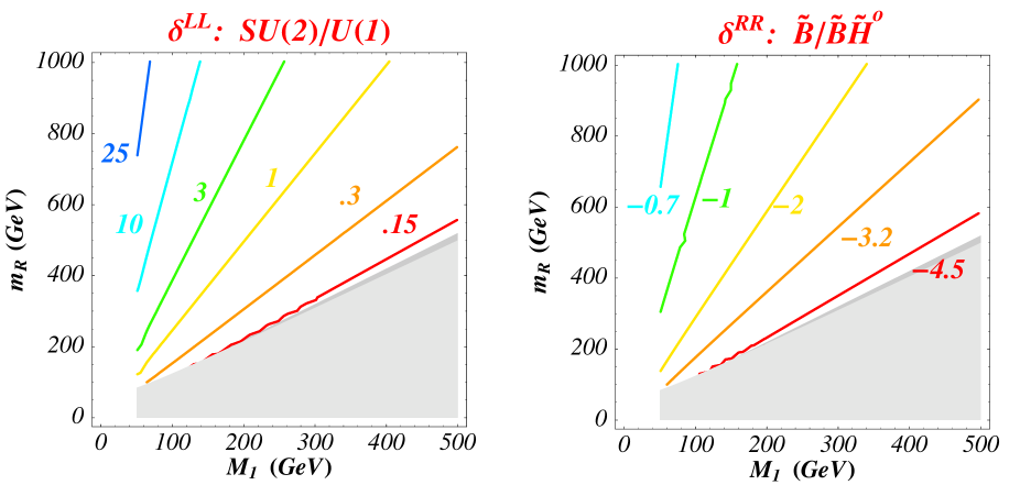
Figure 1: Ratio between the $SU(2)$ and $U(1)$ contributions in the coefficient of $\delta^{LL}$ and between the $\tilde{B}$ and $\tilde{H}\tilde{B}$ contributions in the coefficient of $\delta^{RR}$.

The coefficient of $\delta^{LL}$ receives both $U(1)$ and $SU(2)$-type contributions, respectively from $\tilde{B}$ and $\tilde{B}-\tilde{H}^{0}$ exchange and from $\tilde{W}-\tilde{H}$ exchange. Before discussing the dependences in general supersymmetric scenarios, let us firstly focus on mSUGRA, where no cancellation between the $U(1)$ and $SU(2)$ amplitudes can arise because they have the same sign. Their ratio, $I^{\prime}_{2}/(\eta_{i}I^{\prime}_{B,L}+\frac{1}{2}I^{\prime}_{L})$, is displayed in fig. 1. It can be seen from the figure that if $m_{R}<(>)2.5M_{1}$, then the most important contribution in determining the bound on $\delta^{LL}$ is the $U(1)$ ($SU(2),$ respectively) one. This is quite obvious from the approximation given in the Appendix for the three contributions for $|\mu^{2}|\gg|M_{1}^{2}|$ as in the mSUGRA case:

$$I^{\prime}_{2}+I^{\prime}_{B,L}+\frac{1}{2}I^{\prime}_{L}\approx\frac{M_{2}\cot^{2}\theta_{W}}{M_{1}m_{L}^{2}}\,h_{2}(x^{\prime}_{L})+\frac{\mu^{2}}{2\bar{m}^{4}}\,\left(h_{1}(\bar{x})+k_{1}(\bar{x})\right)+\frac{1}{2m_{L}^{2}}\,h_{1}(x_{L})\\$$

With the gaugino universality relation $M_{2}\approx 2M_{1}\,,$ and neglecting the $k_{1}$ term for simplicity, the region where the $U(1)$ and the $SU(2)$ contributions are commensurate corresponds to the condition $h_{2}(4x_{L})/h_{1}(x_{L})\approx(\mu^{2}+m_{L}^{2})/13m_{L}^{2}\,.$ Then, from the mSUGRA relations (12) one finds $m_{R}^{2}\approx 7M_{1}^{2}\,,$ close to the numerical result. Notice that the ratio between the two $U(1)$ terms, in the region where they are relevant, is $2I^{\prime}_{B,L}/I^{\prime}_{L}\approx\mu^{2}/m_{L}^{2}\,.$ In the dark matter favoured region, $m_{R}^{2}\approx M_{1}^{2}\,,$ and only there, the pure $\tilde{B}$ contribution affords for most of the overall rate (up to 85%). In the opposite situation, $m_{R}^{2}\gg M_{1}^{2}\,,\mu^{2}\sim O(m_{L}^{2})\,,$ $I^{\prime}_{2}/(\eta_{i}I^{\prime}_{B,L}+\frac{1}{2}I^{\prime}_{L})\rightarrow 6.8h_{2}(x_{L})\,,$ which increases with the mass singularity and yields a good approximation in the chargino dominance sector .

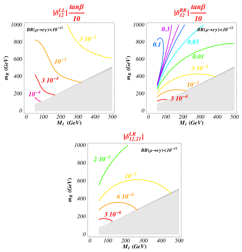
Figure 2: Upper limits on $\delta_{12}$’s in mSUGRA.

If one relaxes even more the mSUGRA constraints, it becomes legitimate to ask if one can escape the LFV limits on $\delta^{LL}$’s or, conversely, how model independent are, e.g. , the more stringent limits on $\delta^{LL}_{12}\,.$ The only possibility is to play with violations of gaugino mass universality. For instance, by reducing $|\mu|$ (i.e., the gluino mass, in current models) the $\tilde{B}-\tilde{H}^{0}$ and $\tilde{W}-\tilde{H}$ contributions increase as $|\mu|^{-2}$, while the $\tilde{B}$ contribution is $|\mu|$ independent. Therefore one needs opposite phases for $M_{2}$ and $M_{1}\,,$ in which case the $\delta^{LL}$’s would remain unconstrained inside a relatively narrow sector of the $(m_{R},M_{1})$ semi-plane.

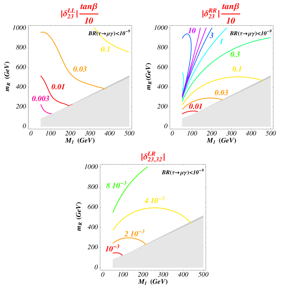
Figure 3: Upper limits on $\delta_{23}$’s in mSUGRA.

In figs. 2 and 3 we show the global bounds on $\delta^{LL}_{12}\tan\beta/10$ and $\delta^{LL}_{23}\tan\beta/10$ that follow from $BR(\mu\rightarrow e\gamma)<10^{-11}$ and $BR(\tau\rightarrow\mu\gamma)<10^{-9}$ respectively. The former corresponds to the present bound (see Table 1). Since the branching ratio is quadratic in the $\delta$’s, the planned improvement by three orders of magnitude on $BR(\mu\rightarrow e\gamma)$ would strengthen the limit by a factor of 30. Notice that the bound decreases quite uniformly as $m_{susy}^{-2}$ thanks to the positive interference among the three contributions.

Instead, $BR(\tau\rightarrow\mu\gamma)<10^{-9}$ is more like a somewhat optimistic prospect. Actually, the present limit on $\delta^{LL}_{23}\tan\beta/10$ is larger by a factor of 30. Thus, depending on $\tan\beta$, $\delta^{LL}_{23}$ is still poorly constrained in most of the mSUGRA parameter space. Here and in the following, we display the bounds corresponding to the planned sensitivity in order to stress the relevance of such an experimental progress. Indeed, at this level, the precision in $\delta^{LL}_{23}$ is at the level of the radiative corrections induced by the seesaw mechanism, providing a unique test for the origin of the atmospheric neutrino oscillations [27]. As for $\tau\rightarrow e\gamma$, the limit on $\delta^{LL}_{13}$ is such that $\delta^{LL}_{13}/\delta^{LL}_{23}=(BR(\tau\rightarrow e\gamma)/BR(\mu\rightarrow e\gamma))^{1/2}$; thus, the present bound on $\delta^{LL}_{13}\tan\beta/10$ is worse by a factor of about 50 with respect to fig. 3.

To stress the importance of considering both the $\tilde{B}$ and the $\tilde{H}-\tilde{W}$ contributions, the bound on $\delta^{LL}_{23}$ is shown in fig. 4 by taking into account only the $\tilde{B}$ or the $\tilde{W}-\tilde{H}$ one (analogous considerations apply for $\mu\rightarrow e\gamma$). The alternate dominance of the $\tilde{B}$ and the chargino contributions according to the value of $M_{1}^{2}/m_{R}^{2}$ is again quite evident. Some of the previous analysis have only considered the chargino part of the $SU(2)$ contribution [28, 27], or only the $\tilde{B}$ contribution .

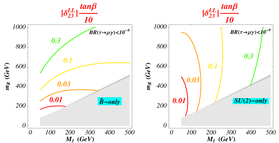
Figure 4: Limits on $\delta_{23}^{LL}\tan\beta/10$ obtained by considering only the $\tilde{B}$ and the $SU(2)$ amplitude respectively.

The chargino dominance when $|\mu|$ is smaller than the slepton masses is an interesting feature since the other mass misalignments leading to LFV, $\delta^{RR}$ and $\delta^{LR}$ are not as effective for this mass pattern. Indeed, as discussed below, the corresponding $\delta^{RR}$ term is somewhat suppressed by negative interference and, generically, the $\delta^{LR}$ term is expected to be proportional to a lepton mass, and furthermore it is of $\tilde{B}$ origin, less enhanced for relatively small $|\mu|$ values than the $\delta^{LL}$ one. Thus, a measurement of, e.g. , the $\mu\rightarrow e\gamma$ decay could be interpreted as a measurement of $\delta^{LL}_{12}\,$ for this mass pattern - and not only an upper bound - if supersymmetry is assumed, or discovered.

3.2 Limits on $\delta^{RR}$

As shown in (22) in the Appendix, the coefficient of the $\delta^{RR}$’s gets only two $U(1)$ contributions, $I^{\prime}_{B(R)}-I^{\prime}_{R}\,,$ with opposite signs - a model independent result that follows from the sign of the hypercharge. Therefore, they can compensate each other in some region of the parameter space, where the limits on the $\delta^{RR}$’s thus become very weak, as we now turn to discuss. Let us write again the approximations in the Appendix as follows:

$$I^{\prime}_{B,R}-I^{\prime}_{R}\approx\frac{\mu^{2}}{2\bar{m}^{4}}\left(h_{1}(\bar{x})+k_{1}(\bar{x})\right)-\frac{1}{m_{R}^{2}}h_{1}(x_{R})$$ (15)

Then the ratio $I^{\prime}_{B,R}/I^{\prime}_{R}$ is $O(1)$ for $\mu^{2}m_{R}^{2}\approx\bar{m}^{4}\,,$ which occurs in mSUGRA for $m_{R}\approx 6M_{1}\,.$ The exact results are shown in fig. 1 b). More generally, one always has a sector in the parameter space, roughly for $|\mu|\approx m_{R}\,,$ where the $\delta^{RR}$’s remain unconstrained or are poorly constrained.

The constraints for $\delta^{RR}_{12}$ are shown in fig. 2 where they clearly become mediocre in the sector where $|\mu|\approx m_{R}\,.$ The same appears in the bounds on $\delta^{RR}_{23}$ shown in fig. 3. As in the previous section, to read the present limit on $\delta^{RR}_{23}$ and $\delta^{RR}_{13}$, the values on the isocurves of fig. 3 have to be increased by a factor of $30$ and $50\,,$ respectively. Thus, by now $\delta^{RR}_{23}$, $\delta^{RR}_{13}$ are not constrained at all.

3.3 Limits on $\delta^{LR}$

Only the pure $\tilde{B}$ graph contributes to $\delta^{LR,RL}_{12}$ and $\delta^{LR,RL}_{23}$ . Their upper limits are displayed in figs. 2 and 3 and they feature a typical $\tilde{B}$ shape in the $(m_{R},M_{1})$ semi-plane. These limits are quite small for $\mu\rightarrow e\gamma$ and the proposed improvement would lower them by a factor of 30. For the present sensitivity to $\tau\rightarrow\mu\gamma$ ($\tau\rightarrow e\gamma$), the numbers on the isocurves have just to be increased by a factor of $30$ ($50\,,$ respectively): it follows that $\delta^{LR,RL}_{23(13)}$ seems already significantly constrained. The shape of the bounds becomes more transparent if one adopts for the $\delta^{LR}$ term the approximation suggested in (22) in the Appendix:

$$\frac{m_{R}m_{L}}{\mu m_{j}\tan\beta}I_{B} \approx \frac{\mu}{m_{R}m_{L}m_{j}\tan\beta}\frac{1}{x_{L}-x_{R}}\left(x_{L}\,g_{1}(x_{L})-x_{R}\,g_{1}(x_{R})\right)$$ (16)

$$\approx \frac{\mu}{m_{j}\bar{m}^{2}\tan\beta}h_{1}(\bar{x})\ ,$$

where the coefficient in front of $I_{B}$ normalizes this term like all others in (22).

The smallness of the bounds should not be misapprehended since, as already recalled, the $\delta^{LR}$’s must be proportional to the Higgs v.e.v., hence to the relevant lepton masses on generic grounds, so that they naturally are at most $O(m_{j}/m_{susy}).$ The factor $\frac{\mu}{m_{j}\tan\beta}$ is taking this fact in account and strengthening the bounds with respect to the chirality non-flip ones. Note that the bounds are not proportional to $\tan\beta$ here.

4 MDM and EDM

If the discrepancy between the experimental value of the muon anomalous MDM [29] and the SM prediction (see for instance [30] and references therein) turns out to be significant, it would signalize new physics, possibly supersymmetry [19, 20, 28]. Actually, the uncertainties are quite close to the level of the contributions that are generically predicted in supersymmetric theories. On the contrary, EDM does not suffer from this problem, since the SM contribution turns out to be far below the potential supersymmetric contribution. By now, only $d_{e}$ gives interesting constraints, while $d_{\mu}$ and $d_{\tau}$ are not yet able to provide significant constraints [21, 22]. However, it has been proposed to increase the sensitivity to $d_{\mu}$ by six and even eight orders of magnitude. This improvement could provide interesting informations to be discussed later on.

In this section we briefly reappraise the constraints on the flavour and CP dependence of the slepton masses coming from the present data on the leptonic MDM and EDM and those prognosticated in future experiments. The supersymmetric contributions to the $a_{i}\,,d_{i}\ (i=e\,,\mu\,,\tau)\,,$ are given by the diagonal elements of (22) which read:

$$\frac{a_{i}}{m_{i}}+\frac{2id_{i}}{e}=\frac{\alpha M_{1}}{4\pi|\mu|^{2}\cos^{2}\theta_{W}}\left[\ m_{i}\mu\tan\beta(I_{B}+\frac{1}{2}I_{L}-I_{R}+I_{2})-A_{i}^{*}m_{i}\,I_{B}\right.\ \ \ \ \ \ \$$

$$+\left.m_{R}m_{L}\left(\delta^{LL}_{ik}\delta^{LR}_{ki}\,I^{\prime}_{B,L}+\delta^{LR}_{ik}\delta^{RR}_{ki}\,I^{\prime}_{B,R}\right)+m_{k}\tan\beta\left(\delta^{LL}_{ik}\delta^{RR}_{ki}\eta^{*}_{k}\mu+\delta^{LR}_{ik}\delta^{LR}_{ki}\eta_{k}\mu^{*}\right)I^{\prime\prime}_{B}\frac{}{}\right]\ \ \$$ (17)

where we identify two kinds of terms:

• FC contributions arising only from the slepton mass parameters that are flavour conserving (in the lepton basis)

• FV contributions involving flavour non-diagonal parameters in the mass matrices, i.e., misalignment.

The first line in (17) contains the terms of FC type, while the FV ones appear in the second line. The latter depend on products of $\delta$’s. All the terms have to be proportional to a lepton mass as emphasized before. However, by their own nature, the FC terms are proportional to the mass of the same fermion, leading to the proportionality between EDM and lepton masses, $d_{i}\propto m_{i}\,,$ and between MDM and the squared lepton masses, $a_{i}\propto m_{i}^{2}\,.$ In the limit where all the slepton masses are flavour independent one has the FC relations:

$$\frac{d_{i}}{d_{j}}=\frac{m_{i}}{m_{j}}\,,\qquad\qquad\frac{a_{i}}{a_{j}}=\frac{m_{i}^{2}}{m_{j}^{2}}\,.$$ (18)

In the development that leads to (17), this is satisfied by the first term and the second FC contribution only violates it by a factor ${A_{i}}/{A_{j}}\,.$ This violation is expected to be too small to significantly change the hierarchy driven by the lepton masses in (18), with the important exception of the LFV and CP phases due to the RGE running [31, 32, 33]. If these were the main contribution to EDM, $d_{\mu}$ should not exceed $3\cdot 10^{-25}$ e cm, due to the present bound on $d_{e}$. Notice that this value roughly corresponds to the planned sensitivity for $d_{\mu}$.

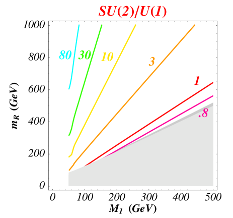
Figure 5: Ratio of the $SU(2)$ and $U(1)$ contributions in mSUGRA. Notice that it is independent on $\tan\beta$.

Instead, some of the FV terms are proportional to a different, possibly heavier lepton mass that break the relation (18) and the corresponding hierarchy in the leptonic MDM/EDM. Thus, even if the FV terms in (17) possess two factors $\delta$’s, they are boosted by $m_{k}/m_{i}$ and could bypass the mass scaling (18), as already discussed in [7, 9] . Therefore, the observation of $d_{\mu}$ above $3\cdot 10^{-25}$ e cm is still a realistic possibility that deserves experimental tests, also because the breaking of the mass scaling rule would be a basic fact in supersymmetric CP violations.

In any case, the experimental limits on the leptonic MDM/EDM shall put upper bounds on the various FC and FV parameters - barring weird cancellations among them. Conversely, the limits on the LFV transitions put limits on the parameters in the FV part of MDM/EDM. We now turn to discuss these limits and their interplay.

4.1 FC contribution to MDM and EDM

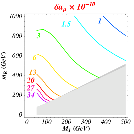
Figure 6: Value of $\delta a_{\mu}$ for $\tan\beta=10$ in mSUGRA.

The FC contributions have been discussed in many recent papers for both the leptonic MDM [19, 20] and EDM [21, 22]. It has been realized that these contributions can be suppressed only by increasing the supersymmetry breaking scale, with the exception of the following two contrived situations far away from the usual mSUGRA constraints: (i) $M_{2}/M_{1}<0$, meaning that $SU(2)$ and $U(1)$ are not simply unified, a possibility offered by some brane models [35]; (ii) a cancellation between the terms with $\mu\tan\beta$ and $A\,,$ involving parameters of different nature. Up to these somewhat contrived possibilities, one can constrain each term separately, as we now discuss.

The main characteristics of the results can be understood from fig. 5 where the $SU(2)$ and the $U(1)$ contributions are compared. They have the same sign if $M_{2}/M_{1}>0$. The $\tilde{B}$ graph becomes comparable to the chargino one only in the region where $\mu^{2}\gg m_{R}^{2}\,,$ i.e., $M_{1}^{2}\sim O(m_{R}^{2})$ in mSUGRA. In this model, the $SU(2)$ and the $U(1)$ contributions become equal for $M_{1}\approx.72m_{R}\,.$ The chargino dominates elsewhere. The approximations given in the Appendix perfectly describe this pattern. Note that only the pure $\tilde{B}$ graph is relevant for the $A-$term input.

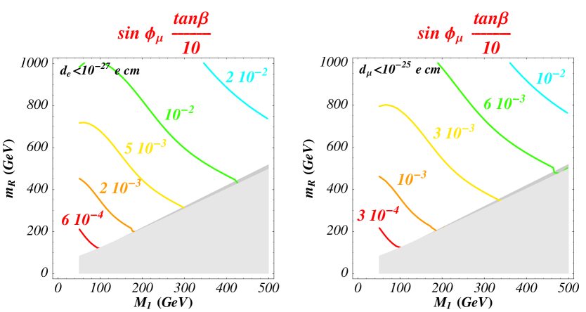
Figure 7: Upper limit on $\sin\phi_{\mu}\tan\beta/10$ in mSUGRA. Vanishing $A$-term is assumed.

Figure 8: Upper limit on $|{\rm Im}A_{e}|/m_{R}$ and $|{\rm Im}A_{\mu}|/m_{R}$.

We refer to the abundant literature for the MDM but for completeness we plot in fig. 6 the contour lines for $a_{\mu}\,.$ Since the naive mass scaling is naturally realized for the FC parameters, $a_{e}=m_{e}^{2}a_{\mu}/m_{\mu}^{2}$ and $a_{\tau}=m_{\tau}^{2}a_{\mu}/m_{\mu}^{2}\,.$ The $A-$term is marginal in this result which corresponds to $\mu\tan\beta\gg A\,.$ When the present theoretical and experimental uncertainties will settle down, this plot will provide interesting constraints. Nevertheless, it should be noted that in the pure chargino approximation one would overlook the constraints close to the dark matter preferred region where the $\tilde{B}$ is important.

As for the leptonic EDM, the upper bounds are separately shown for the two FC terms in (17). We choose phases in such a way that $M_{1}$ is real (and so is $M_{2}$ unless we state the contrary). The relevant phases are then $\phi_{\mu}$ and $\phi_{A}\,,$ respectively. The limits on $\phi_{\mu}$ are shown in fig. 8 for the present limits on $d_{e}$ and they clearly illustrate the so-called supersymmetric CP problem, the experimental requirement of very small CP phases in the soft mass parameters as compared, e.g. , with the Kobaiashi-Maskawa one. The other plot in fig. 8 shows that even with a considerable upgrading of the limits on $d_{\mu}$ one cannot significantly improve the present results on $\phi_{\mu}\,.$ Instead the much better precision in future searches for $d_{e}$ would bring these limits down to extremely small figures.

Let us now assume that $\phi_{\mu}$ satisfies these requirements, and look for the limits on ${\rm Im}A$ that would be obtained with the degree of precision of existing data for $d_{e}$ and the one that has been advertised for projected experiments on $d_{\mu}$. This is shown in fig. 8 for ${\rm Im}A_{e}/m_{R}$ and for ${\rm Im}A_{\mu}/m_{R}$. The curves exhibit a typical $\tilde{B}-$like shape, since this is the only contribution. There are well-known model dependent upper bounds on these parameters to avoid colour and e.m. charge breaking, roughly $|A_{i}|/m_{R}<3$ in mSUGRA. The limits shown in these figures are already much better.

4.2 FV contributions to EDM and MDM

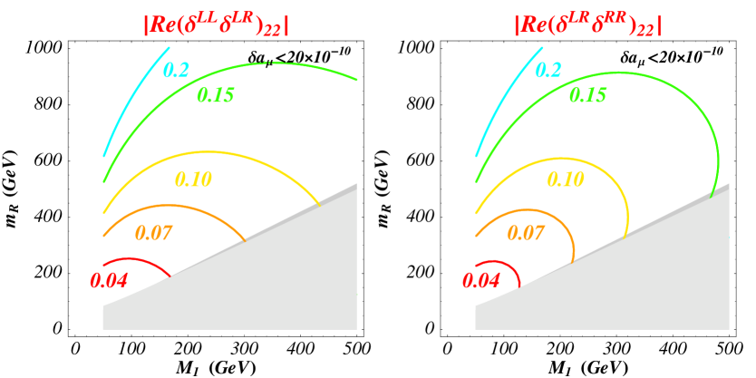
Figure 9: Upper bounds on the real part of products of $\delta$’s obtained by assuming a limit of $20\times 10^{-10}$ on the supersymmetric contribution to $a_{\mu}$.

There are four sums of products of $\delta$’s that are constrained by the limits on MDM and EDM :

$$\delta^{LL}_{ik}\delta^{RR}_{ki}\qquad\delta^{LR}_{ik}\delta^{RR}_{ki}\qquad\delta^{LL}_{ik}\delta^{LR}_{ki}\qquad\delta^{LR}_{ik}\delta^{LR}_{ki}\ .$$ (19)

They are all obtained from the multi-insertion development of the slepton propagator in the pure $\tilde{B}$ graph. Therefore their coefficients are roughly of the same order of magnitude. Approximations are offered in the Appendix that allow for a quick adaptation to other mass configurations. Note that their coefficients include a lepton mass but for $\delta^{LR}_{ik}\delta^{RR}_{ki}$ and $\delta^{LL}_{ik}\delta^{LR}_{ki}$. However, as already stressed, such a factor should be enclosed in $\delta^{LR}_{ik}\,.$ Each product would have two terms since, by assumption, $i\neq k\,.$ However, barring any fortuitous cancellation, each term is constrained by the experimental bounds. We concentrate on those with $k=\tau$ due to the $m_{\tau}$ factor and because the associated $\delta$’s are less constrained by LFV decays. Hence we define $\phi_{\tau}$ as the phase of $(\mu^{*}\tan\beta-A_{\tau})~{},$ close to the phase of $\mu$ for large $\tan\beta~{}.$

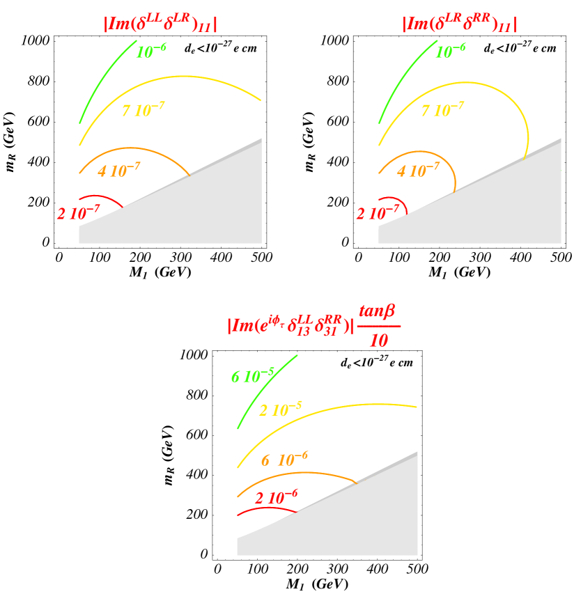
Figure 10: Upper bounds on the imaginary part of products of $\delta$’s with the present limit on $d_{e}$; $\phi_{\tau}$ is defined in the text.

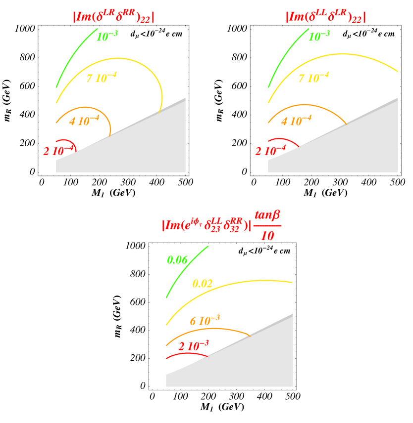
Figure 11: Upper bounds on the imaginary part of products of $\delta$’s for a limit of $10^{-24}$e  cm on $d_{\mu}$; $\phi_{\tau}$ is defined in the text.

The bounds obtained on the real parts by taking into account the present uncertainties in $a_{\mu}$ are shown in fig. 9. Presumably, one cannot do much better because of the level of theoretical uncertainties. Yet, as compared with the results in fig. 3, rescaled to the present experimental bounds on $\tau\rightarrow\mu\gamma$ and $\tau\rightarrow e\gamma\,,$ these products are useful. In particular, they are not proportional to $\mu\tan\beta\,.$

The bounds on the imaginary parts derived from the experimental limits on EDM are free of SM contributions, and depend only on the experimental accuracy. For $d_{e}$ we consider the existent bound and derive the curves in fig. 10 which put limits on the imaginary part of $\delta^{LL}_{13}e^{i\phi_{\tau}}\delta^{RR}_{31}\,,\delta^{LR}_{13}\delta^{RR}_{31}$ and $\delta^{LL}_{13}\delta^{LR}_{31}\,.$ For $d_{\mu}$ we consider the projected precision of $10^{-24}$ e cm and show the results in fig. 11. The limits on $Im(e^{-i\phi_{\tau}}\delta^{LR}_{i3}\delta^{LR}_{3i})$ are not displayed because they are the same as those on $Im(e^{i\phi_{\tau}}\delta^{LL}_{i3}\delta^{RR}_{3i})$. The limits are relatively stringent, even when those involving a $\delta^{LR}$ are increased by a factor $m_{R}/m_{\tau}$ to extract the lepton mass dependence. Notice that the limits on $Im(e^{i\phi_{\tau}}\delta^{LL}_{i3}\delta^{RR}_{3i})$ and $Im(e^{-i\phi_{\tau}}\delta^{LR}_{i3}\delta^{LR}_{3i})$ are inversely proportional to $\mu\tan\beta.$

All these results are easily understood from the approximations in the Appendix, which are also useful for a quick evaluation of alternative models.

5 Limits on FV contributions to EDM from LFV decays

Of course, all these tests of the lepton flavour structure of the soft parameters of supersymmetric extensions of the SM are quite complementary. For instance, as we now turn to discuss, the conjunction of experimental bounds on LFV transitions and on MDM and EDM would help in disentangling the FC and FV contributions in (17) and in learning whether CP violation is more present in one or the other kind of soft masses.

As a case study, we concentrate here on $d_{\mu}$ and evaluate the maximal FV contribution by using the limits on $|\delta^{LL}|\,,|\delta^{RR}|\,,|\delta^{LR}|\,,$ matrix elements obtained from $\tau\rightarrow\mu\gamma$ (those from $\mu\rightarrow e\gamma$ are much smaller and can be neglected). Let us rewrite the sum of the moduli of FV terms contributing to $d_{\mu}$, keeping only $k=\tau\,:$

$$\frac{2d_{\mu}}{e} \leq \frac{\alpha M_{1}}{4\pi|\mu|^{2}\cos^{2}\theta_{W}}\left[\ m_{R}m_{L}\left(|\delta^{LL}_{23}\delta^{LR}_{32}|\,I^{\prime}_{B,L}+|\delta^{LR}_{23}\delta^{RR}_{32}|\,I^{\prime}_{B,R}\right)\right.$$ (20)

$$+ \left.\left(|\delta^{LL}_{23}\delta^{RR}_{32}|+|\delta^{LR}_{23}\delta^{LR}_{32}|\right)|\mu\tan\beta-A^{*}_{\tau}|m_{\tau}I^{\prime\prime}_{B}\frac{}{}\right]$$

This limit is conservative since we replace the imaginary part of the sum by the sum of the moduli. As shown in the Appendix, the integrals $I^{\prime}_{B,L}~{},~{}I^{\prime}_{B,R}~{},~{}I^{\prime\prime}_{B}~{},$ are all of the same order of magnitude. In particular, for $m_{R}>M_{1}$, it can even be approximated in mSUGRA or similar models as

$$\frac{2d_{\mu}}{e} \leq \frac{\alpha M_{1}}{8\pi\bar{m}^{2}\cos^{2}\theta_{W}}\left[\frac{}{}\ \left(|\delta^{LL}_{23}\delta^{LR}_{32}|+|\delta^{LR}_{23}\delta^{RR}_{32}|\right)\right.$$ (21)

$$\left.+2\left(|\delta^{LL}_{23}\delta^{RR}_{32}|+|\delta^{LR}_{23}\delta^{LR}_{32}|\right)|\mu\tan\beta-A^{*}_{\tau}|\frac{m_{\tau}}{\bar{m}^{2}}\right]\,h_{1}(\bar{x})$$

where $\bar{m}^{2}=(m_{L}^{2}+m_{R}^{2})/2$ and $\bar{x}=M_{1}^{2}/\bar{m}^{2}$.

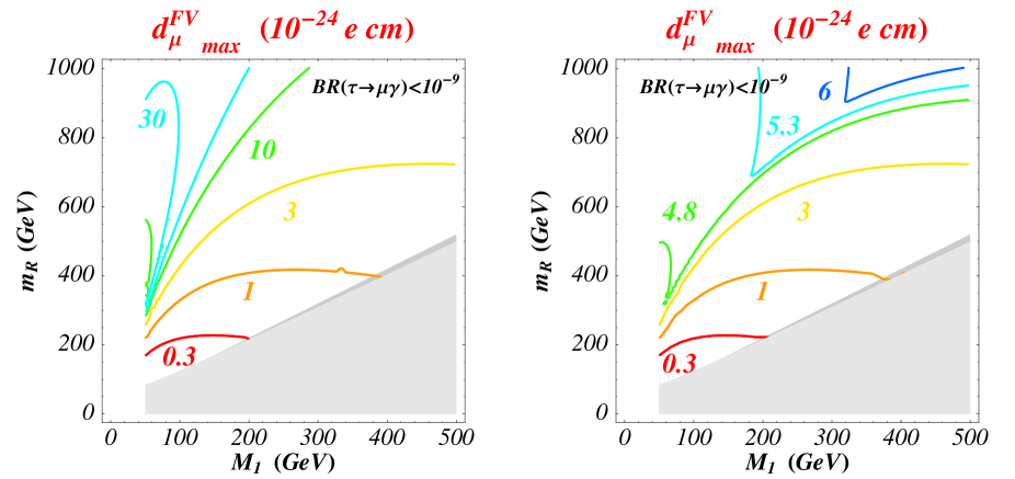
Figure 12: Upper bounds on the FV contribution to $d_{\mu}$ assuming a limit on $\tau\rightarrow\mu\gamma$ at the level of $10^{-9}$. In the left figure the limits on $\delta^{RR}_{23}$ are those from fig. 3 while in the right figure we put an additional upper limit of $0.5$ on them to take into account the way they are defined. Analogous results for $d_{e}$ are discussed in the text.

In section 3, limits on the $|\delta_{23}|$’s were obtained from the experimental bound on ${\rm BR}(\tau\rightarrow\mu\gamma)$ barring important cancellations among the different contributions, i.e.  from eq. (14). In the same spirit, we consider the maximum of the r.h.s. of eq. (20) with eq. (14) as a constraint. Actually, since $|\delta^{RR}_{32}|$ is less constrained than the others, the bound on $d_{\mu}$ come mostly from the term with the product $|\delta^{LR}_{23}\delta^{RR}_{32}|~{}.$ In fig. 12 we have illustrated the kind of bounds on $d_{\mu}$ that are obtained as described, by assuming an experimental limit $BR(\tau\rightarrow\mu\gamma)<10^{-9}~{}.$ As appears from fig. 3, even with such a sensitivity the limits on $|\delta^{RR}_{32}|$ are meaningless in the sector of the $(m_{R},M_{1})$ plane where they are larger than one. The left plot has been obtained by substituting the limits on $|\delta^{RR}_{32}|$ of fig. 3, while the plot on the right is corrected for by the additional condition $|\delta^{RR}_{32}|<1/2~{}$. The latter plot is actually relevant for $BR(\tau\rightarrow\mu\gamma)$ at the level $10^{-9}$, while the first plot is suitable for a quick adaptation of the limits to other levels of sensitivity. Notice that a sensitivity to $\tau\rightarrow\mu\gamma$ at the level of $10^{-9}$ would push down $d_{\mu}^{FV}$, close to the $d_{\mu}$ values that could be tested by the planned experiments in the near future.

If we take the present experimental limit $BR(\tau\rightarrow\mu\gamma)<10^{-6}~{},$ together with a limit of $1/2$ on all the $\delta$’s, we basically get an upper bound on $d_{\mu}$ of the order of few $10^{-22}$ e cm. Therefore we conclude that at present there is still plenty of place for a LFV contribution to $d_{\mu}$ up to three orders of magnitude larger than $m_{\mu}/m_{e}d_{e}$.

For $d_{e}$ there are two FV contributions to be bounded, corresponding to intermediate $\tilde{\mu}$ and $\tilde{\tau}$, respectively. The the limits on the former can be read from those in fig. 12 by multiplying them by $0.2\times 10^{9}~{}{\rm BR}(\mu\rightarrow e\gamma)$ and are close to the present experimental bounds on $d_{e}$ for the existent limits on the $\mu\rightarrow e\gamma$ decay. Instead, for the latter the limits come out much worse, at the level of $10^{9}~{}{\rm BR}(\tau\rightarrow e\gamma)$, namely of those on $d_{\mu}$, since the bounds on $\tau\rightarrow e\gamma$ and $\tau\rightarrow\mu\gamma$ are now very close.

6 Concluding Remarks

The whole set of experimental constraints on the flavour structure of the sleptons masses (in the basis where all interactions are flavour diagonal) are gathered here and displayed in such a way to allow for a ready understanding at both a qualitative and a quantitative level. The bounds on $\mu\rightarrow e\gamma$ transitions are already very constraining in the $\mu-e$ sector and the prospects for the near future are encouraging. As for $\tau\rightarrow\mu\gamma$, the present data are restrictive only at the low side of the sparticle mass spectrum so that any improvement would be particularly welcome.

The searches for the electric dipole moments of the electron and of the muon provide a unique information on the CP violation in the lepton sector. The present data already point to a supersymmetric CP problem similar to what is encountered in the squark sector. The simultaneous analysis of LFV transitions and of the lepton EDM would help discriminating between a CP violation in the flavour blind portion of the supersymmetry breaking parameters or in the presumably richer flavour dependent one. Again, this would require a solid upgrading in the $\tau\rightarrow\mu\gamma$ and $d_{\mu}$ searches to ameliorate the present bounds by a few orders of magnitude.

The level of phenomenological upper bounds on the misalignment parameters, $\delta$’s, that should be reachable in a near future would provide an indirect test of the existence of two kinds of fundamental particles that are too heavy to be more manifest: the right-handed neutrinos from the seesaw mechanism and the triplet partners of the Higgses partners from GUTs. In supersymmetric theories the radiative corrections due to these particles before their decoupling could leave their footprints in the flavour structure of the supersymmetry breaking masses. They are suppressed by loop factors and by the strength of the Yukawa couplings involved, but only logarithmically in their masses. The level of precision of the LFV and even the lepton EDM searches should draw near the one needed to test Yukawa couplings and mass scales of the supersymmetric seesaw and GUT heavy states [31, 28, 27, 36, 33, 37].

At the present and near future level of the experimental precision, the observation of any of the LFV and CP violating transitions discussed in this paper would point to a characteristic scale for these processes around that conjectured for low energy supersymmetry. This is very different from the measured FCNC and CP violating quark transitions that are primarily SM processes, and from the large seesaw scale suggested in the observed LFV in neutrino oscillations. But even a substantial improvement in the upper bounds on any of these processes, especially $\tau\rightarrow\mu\gamma$ decay, would provide decisive data about the flavour and CP violation dependences of the supersymmetry breaking parameters and their origin.

Acknowledgement: We thank O.Vives for pointing out a missing numerical factor in a previous version of the lower plot of fig.2 and some misprint in appendix A.

Appendix A Appendix

A.1 FC and FV Amplitudes

In this Appendix we exhibit the (multiple) insertion approximation for the FC and the FV dipole moment transition amplitude, as discussed in Section 2, where the approximations are defined and justified. They are displayed so as to make more explicit the main dependence on the soft mass parameters and to facilitate a qualitative understanding of the numerical results. The contributions from the different diagrams displayed in Section 2 are separated. They are indicated by the lower indices: $B$ for the pure $\tilde{B}$ diagram, $L$ and $R$ for the $\tilde{B}\,-\,\tilde{H}^{0}$ one with $L$ and $R$ sleptons, respectively, and $2$ for the $\tilde{W}\,-\,\tilde{H}$ ($SU(2)$) one.

$$M_{ij}=2(\mu_{ij}+i\frac{d_{ij}}{e}) = \frac{\alpha M_{1}}{4\pi|\mu|^{2}\cos^{2}\theta_{W}}\ \left\{\ \left[\delta_{ij}m_{j}(\eta_{j}I_{B}+\frac{1}{2}I_{L}-I_{R}+I_{2})\right.\right.$$ (22)

$$-\ \delta^{LL}_{ij}m_{i}(\eta_{i}I^{\prime}_{B,L}+\frac{1}{2}I^{\prime}_{L}+I^{\prime}_{2})\ -\ \delta^{RR}_{ij}m_{j}(\eta_{j}I^{\prime}_{B,R}-I^{\prime}_{R})$$

$$+\ \left.(\delta^{RR}_{ik}\eta_{k}\delta^{LL}_{kj}+\delta^{RL}_{ik}\eta^{*}_{k}\frac{\mu}{\mu^{*}}\delta^{RL}_{kj})m_{k}I^{\prime\prime}_{B}\right]\mu^{*}\tan\beta$$

$$-\ \biggl{.}\Bigl{[}\delta^{RL}_{ij}I_{B}-\delta^{RR}_{ik}\delta^{RL}_{kj}I^{\prime}_{B,R}-\delta^{RL}_{ik}\delta^{LL}_{kj}I^{\prime}_{B,L}\Bigr{]}\,m_{R}m_{L}\ +\ \dots\biggr{\}}$$

where,

$$\eta_{j}=\left(1-\frac{A_{j}}{\mu^{*}\tan\beta}\right)$$ (23)

and terms that are less relevant or higher order are omitted, while we keep terms that could break the proportionality between the dipole moments and the lepton masses for the electron and the muon. In order to define the functions I (22), it is convenient to introduce the new variables:

$$x_{L}=\frac{M_{1}^{2}}{m_{L}^{2}}\qquad x_{R}=\frac{M_{1}^{2}}{m_{R}^{2}}\qquad x^{\prime}_{L}=\frac{|M_{2}|^{2}}{m_{L}^{2}}\qquad y_{L}=\frac{|\mu^{2}|}{m_{L}^{2}}\qquad y_{R}=\frac{|\mu^{2}|}{m_{R}^{2}}$$ (24)

The dependence of the reduced amplitudes $I$’s on the mass parameters is as follows:

$$I_{L}(m_{L}^{2},\,M_{1}^{2},\,\mu^{2}) = \frac{1}{m_{L}^{2}}\frac{y_{L}}{y_{L}-x_{L}}\left[\,g_{1}\left(x_{L}\right)-\,g_{1}\left(y_{L}\right)\right]$$

$$I_{R}(m_{R}^{2},\,M_{1}^{2},\,\mu^{2}) = \frac{1}{m_{R}^{2}}\frac{y_{R}}{y_{R}-x_{R}}\left[\,g_{1}\left(x_{R}\right)-\,g_{1}\left(y_{R}\right)\right]$$

$$I_{2}(m_{L}^{2},\,M_{2}^{2},\,\mu^{2}) = \frac{M_{2}\cot^{2}\theta_{W}}{M_{1}m_{L}^{2}}\frac{y_{L}}{y_{L}-x^{\prime}_{L}}\left[\,g_{2}\left(x^{\prime}_{L}\right)-\,g_{2}\left(y_{L}\right)\right]$$

$$I_{B}(M_{1}^{2},\,m_{L}^{2},\,m_{R}^{2}) = \frac{1}{m_{R}^{2}-m_{L}^{2}}\left[y_{L}\,g_{1}\left(x_{L}\right)-y_{R}\,g_{1}\left(x_{R}\right)\right]$$

$$I^{\prime}_{L}(m_{L}^{2},\,M_{1}^{2},\,\mu^{2}) = \frac{1}{m_{L}^{2}}\frac{y_{L}}{y_{L}-x_{L}}\left[\,h_{1}\left(x_{L}\right)-\,h_{1}\left(y_{L}\right)\right]$$

$$I^{\prime}_{R}(m_{R}^{2},\,M_{1}^{2},\,\mu^{2}) = \frac{1}{m_{R}^{2}}\frac{y_{R}}{y_{R}-x_{R}}\left[\,h_{1}\left(x_{R}\right)-\,h_{1}\left(y_{R}\right)\right]$$

$$I^{\prime}_{2}(m_{L}^{2},\,M_{2}^{2},\,\mu^{2}) = \frac{M_{2}\cot^{2}\theta_{W}}{M_{1}m_{L}^{2}}\frac{y_{L}}{y_{L}-x^{\prime}_{L}}\left[\,h_{2}\left(x^{\prime}_{L}\right)-\,h_{2}\left(y_{L}\right)\right]$$

$$I^{\prime}_{B,R}(M_{1}^{2},\,m_{L}^{2},\,m_{R}^{2}) = -\frac{1}{m_{R}^{2}-m_{L}^{2}}\left(y_{R}\,h_{1}\left(x_{R}\right)-m_{R}^{2}I_{B}\right)$$

$$I^{\prime}_{B,L}(M_{1}^{2},\,m_{L}^{2},\,m_{R}^{2}) = -\frac{1}{m_{L}^{2}-m_{R}^{2}}\left(y_{L}\,h_{1}\left(x_{L}\right)-m_{L}^{2}I_{B}\right)$$

$$I^{\prime\prime}_{B}(M_{1}^{2},\,m_{L}^{2},\,m_{R}^{2}) = -\frac{m_{L}^{2}m_{R}^{2}}{m_{L}^{2}-m_{R}^{2}}\left(\frac{1}{m^{2}_{L}}I^{\prime}_{B,L}-\frac{1}{m^{2}_{R}}I^{\prime}_{B,R}\right)$$ (25)

where the (factorized) loop integrals have the following expressions:

$$\begin{array}[]{cc}g_{1}(x)=\frac{1-x^{2}+2x\ln(x)}{(1-x)^{3}}&g_{2}(x)=\frac{x^{2}-8x+7+2(2+x)\ln(x)}{2(x-1)^{3}}\\ h_{1}(x)=\frac{1+4x-5x^{2}+(2x^{2}+4x)\ln(x)}{(1-x)^{4}}&h_{2}(x)=\frac{7x^{2}+4x-11-2(x^{2}+6x+2)\ln(x)}{2(x-1)^{4}}\end{array}$$ (26)

These functions are plotted in Fig. 13. Note that for very small $x,$ $\,g_{1},\,\,h_{1}\,\rightarrow 1\,,$ and that $g_{1}(1/x)=xg_{1}(x)~{}.$ Because of the chargino mass singularity, $\,g_{2},\,\,h_{2}\,\sim\ln x^{-2}\,$ near the origin; this increases the relative $SU(2)$ contributions for $m_{L}^{2}\,\gg|M_{2}|^{2}\,.$ Within the $SU(2)$ diagrams, only the chargino part has the logarithmic divergence and it dominates its opposite sign $SU(2)$ neutralino counterpart everywhere. Also, $\,h_{1},\,\,h_{2}\,,$ which appear in the FV amplitudes, decrease much faster than $\,g_{1},\,\,g_{2}$ which appear in the FC amplitudes, since they have an additional slepton propagator in the insertion approximation.

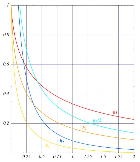
Figure 13: The functions $g_{i}(x)~{},h_{i}(x)$ and $k_{1}(x)$.

A.2 Approximate Expressions

There are several approximations that could be useful to understand the behaviour of the FC and FV processes as shown in the figures. In many cases they can also help to extrapolate the results in these figures to values of the parameters that deviate form the mSUGRA constraints.

First consider the case with $\mu^{2}\,\gg M_{2}^{2},\,M_{1}^{2}$ which appears in mSUGRA and all models where $\mu^{2}$ is tuned to the gluino masses by the vacuum condition. Then, one can use the simplified expressions:

$$I_{L}\approx\frac{g_{1}\left(x_{L}\right)}{m_{L}^{2}}\,,\qquad I_{R}\approx\frac{g_{1}\left(x_{R}\right)}{m_{R}^{2}}\,,\qquad I_{2}\approx\left(\frac{M_{2}\cot^{2}\theta_{W}}{M_{1}}\right)\frac{g_{2}\left(x^{\prime}_{L}\right)}{m_{L}^{2}}\,,$$

$$I^{\prime}_{L}\approx\frac{h_{1}\left(x_{L}\right)}{m_{L}^{2}}\,,\qquad I^{\prime}_{R}\approx\frac{h_{1}\left(x_{R}\right)}{m_{R}^{2}}\,,\qquad I^{\prime}_{2}\approx\left(\frac{M_{2}\cot^{2}\theta_{W}}{M_{1}}\right)\frac{h_{2}\left(x^{\prime}_{L}\right)}{m_{L}^{2}}\,,$$ (27)

and the approximate relations:

$$I_{B}\approx\frac{\mu^{2}}{m_{R}^{2}-m_{L}^{2}}\left(I_{L}-I_{R}\right)\qquad I^{\prime\prime}_{B}\approx\frac{m_{R}^{2}m_{L}^{2}}{(m_{R}^{2}-m_{L}^{2})^{2}}\left(y_{R}I^{\prime}_{R}+y_{L}I^{\prime}_{L}-2I_{B}\right)$$

$$I^{\prime}_{B,R}\approx-\frac{m_{R}^{2}}{m_{R}^{2}-m_{L}^{2}}\left(y_{R}I^{\prime}_{R}-I_{B}\right)\qquad I^{\prime}_{B,L}\approx-\frac{m_{L}^{2}}{m_{L}^{2}-m_{R}^{2}}\left(y_{L}I^{\prime}_{L}-I_{B}\right)\,.$$ (28)

If $m_{R}^{2}$ and $m_{L}^{2}$ are not very different these expressions can be further approximated as,

$$I_{B}\approx\frac{\bar{y}~{}h_{1}(\bar{x})}{\bar{m}^{2}}\qquad I^{\prime}_{B,R}\approx I^{\prime}_{B,L}\approx\frac{\bar{y}~{}(h_{1}(\bar{x})+k_{1}(\bar{x}))}{2\bar{m}^{2}}\qquad I^{\prime\prime}_{B}\approx\frac{\bar{y}~{}(h_{1}(\bar{x})+2k_{1}(\bar{x}))}{3\bar{m}^{2}}$$ (29)

where $\,k_{1}(x)=d\,(xh_{1})/dx\,,$ is very small everywhere except close to the origin, $\bar{m}^{2}=(m_{R}^{2}+m_{L}^{2})/2\,,\bar{x}=M_{1}^{2}/\bar{m}^{2}\,,\bar{y}=|\mu^{2}|/\bar{m}^{2}\,.$

A.3 Special regions in mSUGRA

One can understand the trend of several of the results presented in the figures by considering further approximations in the framework of mSUGRA or similar. Let us first consider the ratio between the different contributions to the FC component of (22) as obtained from (A.2, 28):

$$\frac{I_{B}}{\frac{1}{2}I_{L}-I_{R}}\approx\frac{2\mu^{2}\left(I_{L}-I_{R}\right)}{\left(m_{R}^{2}-m_{L}^{2}\right)\left(I_{L}-2I_{R}\right)}\approx-\frac{2\mu^{2}\,h_{1}(\bar{x})}{\bar{m}^{2}\,g_{1}(x_{R})}$$ (30)

where $1>h_{1}(x)/g_{1}(x)>1/2$ for $0<x<1\,.$ From the mSUGRA expression for $\mu^{2}$ in terms of $m_{R}^{2}$ and $M_{1}^{2}\,,$ (12), one gets that the $U(1)$ contribution, $I_{B}+I_{L}/2-I_{R}\,,$ does not changes sign in the region of physical interest. The ratio between the $SU(2)$ and the $U(1)$ amplitudes is:

$$\frac{I_{2}}{I_{B}+\frac{1}{2}I_{L}-I_{R}}\approx\left(\frac{M_{2}\cot^{2}\theta_{W}}{M_{1}m_{L}^{2}}\right)\frac{\bar{m}^{2}\,g_{2}(x^{\prime}_{L})}{\mu^{2}\,h_{1}(\bar{x})-\frac{1}{2}\bar{m}^{2}\,g_{1}(\bar{x})}$$ (31)

which shows that the chargino term dominates over the neutralino one as far as $m_{R}^{2}\gg M_{1}^{2}\,.$ Let us now consider the mSUGRA region of cosmological interest, $m_{R}^{2}\approx M_{1}^{2}\,,\ m_{L}^{2}\approx 3M_{1}^{2}\,,\mu^{2}\approx 20M_{1}^{2}\,,$. Therein, one has within the approximations given by (A.2) and (28)

$$I_{L}\approx 0.17\,{M_{1}^{-2}}\qquad I_{R}\approx 0.33\,{M_{1}^{-2}}\qquad I_{B}\approx 1.7\,{M_{1}^{-2}}\qquad I_{2}\approx 1.05\,M_{1}^{-2}$$ (32)

so that the dominant amplitude is $I_{B}\,.$ In particular, the ratio between the $SU(2)$ and the $U(1)$ contributions is $0.72$, as shown in Fig. (5). Notice that the $I_{B}$ dominance in this regime of mSUGRA is mainly due to the large value of $\mu^{2}\,.$

The analysis of the FV terms is analogous.

References

- [1] Super-Kamiokande Collaboration, Phys. Rev. Lett. 81 (1998) 1562; Phys. Rev. Lett. 85 (2000) 3999; Phys. Rev. Lett. 86 (2001) 5656, hep-ex/0103033; SNO Collaboration, Phys. Rev. Lett. 87 (2001) 71301, nucl-ex/0106015.
- [2] L.J. Hall, V.A. Kostelecky and S. Raby, Nucl. Phys. B 267 (1986) 415; F. Gabbiani and A. Masiero, Nucl. Phys. B 322 (1989) 235.
- [3] F. Gabbiani, E. Gabrielli, A. Masiero and L. Silvestrini, Nucl. Phys. B 477 (1996) 321, hep-ph/9604387.
- [4] J. Hisano, T. Moroi, K. Tobe, M. Yamaguchi and T. Yanagida, Phys. Lett. B 357 (1995) 579, hep-ph/9501407; J. Hisano, T. Moroi, K. Tobe and M. Yamaguchi, Phys. Rev. D 53 (1996) 2442, hep-ph/9510309; J. Hisano and D. Nomura, Phys. Rev. Ḏ 59 (1999) 116005, hep-ph/9810479.
- [5] T. Moroi, Phys. Rev. D 53 (1996) 6565, hep-ph/9512396; Erratum-ibid. D 56 (1997) 4424.
- [6] S. Pokorski, J. Rosiek and C.A. Savoy, Nucl. Phys. B 570 (2000) 81, hep-ph/9906206.
- [7] J.L. Feng, K.T. Matchev and Y. Shadmi, Nucl. Phys. B 613 (2001) 366, hep-ph/0107182.
- [8] F. Borzumati and A. Masiero, Phys. Rev. Lett. 57 (1986) 961.
- [9] A. Romanino and A. Strumia, Nucl. Phys. B 622 (2002) 73, hep-ph/0108275.
- [10] E.D. Commins, S.B. Ross, D. Demille, B.C. Regan, Phys. Rev. A 50 (1994) 2960.
- [11] B.E. Sauer, talk at Charm, Beauty and CP, 1st Int. Workshop on Frontier Science, October 6-11, 2002, Frascati, Italy.
- [12] S.K. Lamoreaux, nucl-ex/0109014.
- [13] CERN-Mainz-Daresbury Collaboration, Nucl. Phys. B 150 (1979) 1.
- [14] R. Carey et al., Letter of Intent to BNL (2000); Y.K. Semertzidis et al., hep-ph/0012087.
- [15] J. Aysto et al., hep-ph/0109217.
- [16] Particle Data Book, Phys. Rev. D 66 (2002) 10001.
- [17] L.M. Barkov et al., proposal for an experiment at PSI, http://meg.web.psi.ch.
- [18] I. Hinchliffe, F.E. Paige, Phys. Rev. D 63 (2001) 115006, hep-ph/0010086; D.F. Carvalho, J.R. Ellis, M.E. Gomez, S. Lola and J.C. Romao, hep-ph/0206148; J. Kalinowski, hep-ph/0207051.
- [19] M. Carena, G.F. Giudice and C.E.M. Wagner, Phys. Lett. B 390 (1997) 234, hep-ph/9610233; E. Gabrielli and U. Sarid, Phys. Rev. Lett. 79 (1997) 4752, hep-ph/9707546.
- [20] J.L. Feng and K.T. Matchev, Phys. Rev. Lett. 86 (2001) 3480, hep-ph/0102146; L. Everett, G.L. Kane, S. Rigolin and L. Wang, Phys. Rev. Lett. 86 (2001) 3484, hep-ph/0102145; T. Ibrahim, U. Chattopadhyay and P. Nath, Phys. Rev. D 64 (2001) 016010, hep-ph/0102324; J. Ellis, D.V. Nanopoulos and K.A. Olive, Phys. Lett. B 508 (2001) 65, hep-ph/0102331 S. Komine, T. Moroi and M. Yamaguchi, Phys. Lett. B 507 (2001) 224, hep-ph/0103182; Z. Chacko and G.D. Kribs, Phys. Rev. D 64 (2001) 75015, hep-ph/0104317; D.G. Cerdeno, E. Gabrielli, S. Khalil, C. Munoz and E. Torrente-Lujan, Phys. Rev. D 64 (2001) 093012, hep-ph/0104242; U. Chattopadhyay and P. Nath, hep-ph/0208012; S.P. Martin, J.D. Wells, hep-ph/0209309.
- [21] T. Ibrahim and P. Nath, Phys. Rev. D 58 (1998) 111301, hep-ph/9807501; T. Falk and K. Olive, Phys. Lett. B 439 (1998) 71; M. Brhlik, G. Good and G.L. Kane, Phys. Rev. D 59 (1999) 115004, hep-ph/9810457;
- [22] U. Chattopadhyay, T. Ibrahim and P. Roy, Phys. Rev. D 64 (2001) 013004, hep-ph/0012337; V. Barger et al., hep-ph/0101106; S. Abel, S. Khalil and O. Lebedev, Nucl. Phys. B 606 (2001) 151, hep-ph/0103320; T. Ibrahim and P. Nath, Phys. Rev. D 64 (2001) 093002, hep-ph/0105025.
- [23] J. Ellis, T. Falk and K.A. Olive, Phys. Lett. B 444 (1998) 367, hep-ph/9810360; J. Ellis, T. Falk, G. Ganis and K.A. Olive, Phys. Rev. D 62 (2000) 075010, hep-ph/0004169; J. Ellis, D.V. Nanopoulos and K.A. Olive, Phys. Lett. B 508 (2001) 65, hep-ph/0102331; U. Chattopadhyay, A. Corsetti and P. Nath, Phys. Rev. D 66 (2002) 035003, hep-ph/0201001.
- [24] R. Kitano, M. Koike and Y. Okada, hep-ph/0203110.
- [25] J. Kaulard et al., Phys. Lett. B 422 (1998) 334.
- [26] M. Bachman et al., (1997) http://meco.ps.uci.edu.
- [27] S. Lavignac, I. Masina and C.A. Savoy, Phys. Lett. B 520 (2001) 269, hep-ph/0106245.
- [28] D.F. Carvalho, J. Ellis, M.E. Gomez and S. Lola, Phys. Lett. B 515 (2001) 323, hep-ph/0103256.
- [29] G.W. Bennett, et al., Muon g-2 Collaboration, Phys. Rev. Lett. 89 (2002) 101804; Erratum-ibid. 89 (2002) 129903, hep-ex/0208001.
- [30] M. Davier, S. Eidelman, A. Hocker and Z. Zhang, hep-ph/0208177.
- [31] J. Ellis, J. Hisano, S. Lola and M. Raidal, Nucl. Phys. B 621 (2002) 208, hep-ph/0109125; J. Ellis, J. Hisano, M. Raidal and Y. Shimizu, Phys. Lett. B 528 (2002) 86, hep-ph/0111324; J. Ellis and M. Raidal, Nucl. Phys. B 643 (2002) 229, hep-ph/0206174.
- [32] I. Masina, hep-ph/0210125.
- [33] I. Masina and C.A. Savoy, in preparation.
- [34] P. Brax and C.A. Savoy, Nucl. Phys. B 447 (1995) 227, hep-ph/9503306.
- [35] M. Brhlik, L. Everett, G. L. Kane and J. Lykken, Phys. Rev. D 62 (2000) 035005, hep-ph/9908326; Phys. Rev. Lett. 83 (1999) 2124, hep-ph/9905215.
- [36] R. Rattazzi and U. Sarid, Nucl. Phys. B 475 (1996) 27, hep-ph/9512354; W. Buchmuller, D. Delepine and F. Vissani, Phys. Lett. B 459 (1999) 171, hep-ph/9904219; J. L. Feng, Y. Nir and Y. Shadmi, Phys. Rev. D61 (2000) 113005, hep-ph/9911370; J. Ellis, M.E. Gomez, G.K. Leontaris, S.Lola and D.V. Nanopoulos, Eur. Phys. J. C 14 (2000) 319, hep-ph/9911459 K. S. Babu, B. Dutta and R. N. Mohapatra, Phys. Lett. B458 (1999) 93; W. Buchmuller, D. Delepine and L. T. Handoko, Nucl. Phys. B576 (2000) 445; J. Sato, K. Tobe and T. Yanagida, Phys. Lett. B 498 (2001) 189, hep-ph/0010348; J. Hisano and K. Tobe, Phys. Lett. B 510 (2001) 197, hep-ph/0102315 J.A. Casas and A. Ibarra, Nucl. Phys. B 618 (2001) 171, hep-ph/0103065; S. Davidson and A. Ibarra, JHEP 0109 (2001) 013, hep-ph/0104076; T. Blazek and S.F. King, Phys. Lett. B 518 (2001) 109, hep-ph/0105005; S. Lavignac, I. Masina and C.A. Savoy, Nucl. Phys. B 633 (2002) 139, hep-ph/0202086; A. Masiero, S.K. Vempati and O. Vives, hep-ph/0209303.
- [37] R. Barbieri and L. Hall, Phys. Lett. B 338 (1994) 212, hep-ph/9408406; R. Barbieri, L. Hall and A. Strumia, Nucl. Phys. B 445 (1995) 219, hep-ph/9501334; R. Barbieri, A. Romanino and A. Strumia, Phys. Lett. B 369 (1996) 283, hep-ph/9511305 A. Romanino and A. Strumia, Nucl. Phys. B 490 (1997) 3, hep-ph/9610485.