Transport Coefficients at Leading Order: Kinetic Theory versus Diagrams

Abstract

I review what is required to compute transport coefficients in ultra-relativistic, weakly coupled gauge theories, at leading order in $g$, using kinetic theory. Then I discuss how the calculation would look in alternative approaches: the 2PI method, and direct diagrammatic analysis. I argue that the 2PI method may be a good way to derive the kinetic theory, but is not very useful directly (in a gauge theory). The diagrammatic approach is almost hopeless.

1 Introduction

A “big question” in particle physics at extreme energy densities (Strong and Electroweak Matter, the topic of this conference), is how nonequilibrium systems behave. Here I will only talk about weak coupling, plus some conditions on the departure from equilibrium and the measurables of interest, which allow application of techniques grounded in perturbative field theory. (Some very interesting questions are excluded by this condition; but the problems included are interesting and challenging.) In particular, I am going to talk about transport coefficients, even though they represent the “closest to equilibrium” nonequilibrium systems we could consider.

Transport coefficients tell about equilibration in systems which are homogeneous on fairly large scales, and are locally fairly close to equilibrium. The traditional approach to dealing with such a system at weak coupling is kinetic theory, that is, Boltzmann equations. We have recently presented[1] a Boltzmann equation which is adequate for treating transport coefficients in a nonabelian gauge theory at leading order in the coupling $g$ (see also Larry Yaffe’s talk in this proceeding). Its applicability extends well beyond the near-equilibrium situation needed for transport, though the homogeneity requirements for the equation to apply are stronger than you might naively guess.

But there has been much interest in addressing transport using other tools, particularly the 2PI formalism and direct diagrammatic analysis. I will argue that, if the goal is to perform a calculation in a gauge theory, which is complete at leading order in the gauge coupling $g$, then both methods become very complicated. The 2PI formalism may be a very efficient way of deriving the correct Boltzmann equation, but direct application without gradient expansion–for instance, numerically, as has recently been done in scalar field models[2, 3, 4]–will encounter substantial difficulties. The diagrammatic approach at leading order appears to be so complicated that I see little reason to pursue this method further.

2 Boltzmann approach to transport coefficients

When a plasma is sufficiently homogeneous, the large scale flow is accurately described by ideal hydrodynamics. Under ideal hydrodynamic behavior, entropy is conserved; particle number is often approximately conserved. In the heavy ion context, this means that almost all the available energy of the system goes into bulk flow.

Transport coefficients give the first corrections to this behavior, when the system is large but not infinitely large. They cause entropy generation, and tell how close to local thermal equilibrium the system remains. In the context of heavy ion collisions, knowing the transport coefficients could tell us when the hydrodynamic approximation has broken down, which would help hydro simulators to know when to impose chemical and kinetic freeze-out. In early universe physics, diffusion coefficients are useful in baryogenesis calculations, and viscosity and diffusion coefficients can indicate how far around electroweak bubble walls the departure from equilibrium extends. For the “pure” theory of thermal field theory, transport coefficients are a useful object of study because their definition is very theoretically clean. If we want to develop the tools to study nonequilibrium problems in a controlled way, those tools should be able to tell us the values of transport coefficients. So being able to compute them is the most basic step towards more general nonequilibrium calculations.

In the Boltzmann approach, one shows (or assumes, or hopes) that the plasma is well described as a bath of long lived quasiparticles, which undergo occasional and relatively localized scatterings. That is, one requires that the interesting observables are dominated by the two point function, that the spectral weight for the two point function is tightly peaked, that the evolution of the two point function can be accurately written in terms of scatterings with the other quasiparticles, and that these scattering processes are local on the scale of the spatial variation of the system.

Given these conditions, one can write down a Boltzmann equation,

$$\partial_{t}f({\bm p},{\bm x},t)+\frac{{\bm p}}{p^{0}}\cdot\partial_{{\bm x}}f({\bm p},{\bm x},t)+{\bm F}\!\cdot\partial_{\bm p}f({\bm p},{\bm x},t)=-{\mathcal{C}}[f]\,,$$ (1)

with ${\mathcal{C}}$ the collision operator. Applying this to a situation where $f$ is spatially inhomogeneous, or where the force term represents an electrical field, allows calculation of transport coefficients. In particular, when $f$ exhibits shear flow, then computing the traceless part of the stress tensor gives the shear viscosity,

$$T_{ij}[f]-\frac{1}{3}\delta_{ij}T_{kk}[f]=\eta\left(\partial_{i}v_{j}+\partial_{j}v_{i}-\frac{2}{3}\delta_{ij}\partial_{k}v_{k}\right)\,.$$ (2)

Similarly, the diffusion constant is determined by the size of a conserved current, when the number density varies in space. In each case, one must solve for $f$ (at linearized order in the departure from local equilibrium) in the Boltzmann equation. This is hard because it is an integral equation; the operator ${\mathcal{C}}[f]$ contains $f$ at momenta other than ${\bm p}$. It is especially hard because, at leading order, ${\mathcal{C}}$ turns out to be quite nasty!

The collision operator ${\mathcal{C}}$ should include “all collision processes which are important at leading order.” At leading log order, there are only a few processes; $t$ channel boson exchange, Compton scattering, and an annihilation process related to Compton by crossing. Further, simplifying approximations can be made to each collision term, which in fact makes the collision operator a differential operator, not an integral one[1]. But at leading order, in fact at next-to-leading-logarithm, one needs not only all $2\leftrightarrow 2$ processes, but certain inelastic LPM suppressed splitting processes[5]. For the full details see[5, 6, 7]. To show how bad the situation is, I will write ${\mathcal{C}}$ in some detail, though not enough to allow you to evaluate it: The $2\leftrightarrow 2$ piece is

$${\mathcal{C}}^{2\leftrightarrow 2}_{a}[f] = \frac{1}{4|{\bm p}|\nu_{a}}\sum_{bcd}\int_{{\bm k}{\bm p}^{\prime}{\bm k}^{\prime}}\!\!\left|{\mathcal{M}}^{ab}_{cd}({\bm p},{\bm k};{\bm p}^{\prime},{\bm k}^{\prime})\right|^{2}\!(2\pi)^{4}\delta^{(4)}(P{+}K{-}P^{\prime}{-}K^{\prime})$$ (3)

$$\times\Bigl{\{}f_{a}({\bm p})\,f_{b}({\bm k})\,[1{\pm}f_{c}({\bm p}^{\prime})]\,[1{\pm}f_{d}({\bm k}^{\prime})]-[(p,k)\leftrightarrow(p^{\prime},k^{\prime})]\Bigl{\}}\,.$$

The $2\leftrightarrow 2$ matrix elements should be summed over incoming and outgoing spins and colors; literature values, summed only over outgoing states, are available[8]. But in addition, HTL corrections are needed on some internal lines, which means that the form of certain matrix elements is more complicated than in vacuum[5]. But the real problem is the inelastic LPM suppressed splitting processes:

$${\mathcal{C}}^{``1\leftrightarrow 2"}_{a}[f] = \frac{(2\pi)^{3}}{2|{\bm p}|^{2}\nu_{a}}\sum_{b,c}\int_{0}^{\infty}dp^{\prime}\>dk^{\prime}\;\delta(|{\bm p}|-p^{\prime}-k^{\prime})\;\gamma^{a}_{bc}({\bm p};p^{\prime}\,\hat{\bm p},k^{\prime}\,\hat{\bm p})$$ (4)

$$\hskip 40.00006pt\times\Bigl{\{}f_{a}({\bm p})[1\pm f_{b}(p^{\prime}\,\hat{\bm p})][1\pm f_{c}(k^{\prime}\,\hat{\bm p})]-[f\leftrightarrow(1{\pm}f)]\Bigr{\}}$$

$$+\frac{(2\pi)^{3}}{|{\bm p}|^{2}\nu_{a}}\sum_{b,c}\int_{0}^{\infty}dk\>dp^{\prime}\;\delta(|{\bm p}|+k-p^{\prime})\;\gamma_{ab}^{c}(p^{\prime}\,\hat{\bm p};{\bm p},k\,\hat{\bm p})$$

$$\hskip 40.00006pt\times\Bigl{\{}f_{a}({\bm p})f_{b}(k\,\hat{\bm p})[1\pm f_{c}(p^{\prime}\,\hat{\bm p})]-[f\leftrightarrow(1{\pm}f)]\Bigr{\}}\,.$$

The awfulness is hiding in $\gamma^{a}_{bc}(\ldots)$; evaluating it requires solving an integral equation. For instance, for $q\leftrightarrow qg$ processes, it is

$$\gamma^{q}_{qg}(p{\hat{\bm n}};p^{\prime}{\hat{\bm n}},k{\hat{\bm n}}) = \frac{p^{\prime}{}^{2}+p^{2}}{p^{\prime}{}^{2}\,p^{2}\,k^{3}}\>{\mathcal{F}}_{\rm q}^{\hat{\bm n}}(p,p^{\prime},k)\,,$$

$${\mathcal{F}}_{\rm q}^{\hat{\bm n}}(p,p^{\prime},k) \equiv \frac{d_{\rm F}C_{\rm F}\alpha_{\rm s}}{2(2\pi)^{3}}\int\frac{d^{2}{\bm h}}{(2\pi)^{2}}\;2{\bm h}\cdot{\rm Re}{\bf F}_{s}^{\hat{\bm n}}({\bm h};p,p^{\prime},k)\,,$$

$$2{\bm h} = i\,\delta E\,{\bm F}_{s}^{\hat{\bm n}}({\bm h})+g^{2}T\int\frac{d^{2}{\bm q}_{\perp}}{(2\pi)^{2}}\left(\frac{1}{{\bm q}_{\perp}^{2}}-\frac{1}{{\bm q}_{\perp}^{2}+m_{\rm D}^{2}}\right)$$

$$\hskip 36.135pt\times\biggl{\{}(C_{s}-{\textstyle\frac{1}{2}}C_{\rm A})\left[{{\bm F}}_{s}^{\hat{\bm n}}({\bm h})-{{\bm F}}_{s}^{\hat{\bm n}}({\bm h}{-}k\,{\bm q}_{\perp})\right]$$

$$\hskip 75.88371pt+{\textstyle\frac{1}{2}}C_{\rm A}\left[{{\bm F}}_{s}^{\hat{\bm n}}({\bm h})-{{\bm F}}_{s}^{\hat{\bm n}}({\bm h}{+}p\,{\bm q}_{\perp})\right]$$

$$\hskip 75.88371pt+{\textstyle\frac{1}{2}}C_{\rm A}\left[{{\bm F}}_{s}^{\hat{\bm n}}({\bm h})-{{\bm F}}_{s}^{\hat{\bm n}}({\bm h}{-}p^{\prime}{\bm q}_{\perp})\right]\biggr{\}}$$

$$\delta E = \frac{m_{{\rm eff,g}}^{2}}{2k}+\frac{m_{{\rm eff,q}}^{2}}{2p^{\prime}}-\frac{m_{{\rm eff,q}}^{2}}{2p}+\frac{{\bm h}^{2}}{2p\,k\,p^{\prime}}\,.$$ (5)

That is, there is an integral equation just to determine the coefficient in one of the collision terms, which itself appears in an integral equation for the expression that we want.

3 Alternate approaches

For some reason, people don’t like the Boltzmann approach. The obvious reason is that it involves solution of an integral equation (in fact, at leading order, an integral equation within an integral equation). This objection is probably not well grounded, because other approaches presumably reduce to the same integral equation, in one guise or another. But there are some deeper, more philosophical reasons people don’t like the Boltzmann approach.

One problem is that people don’t trust it. Where is the careful derivation? How do you know you have not missed some necessary term in the collision integral? What about quantum and high gradient effects? What do you do when the particle widths are large? Another problem people have is that the Boltzmann approach is old fashioned. Boltzmann was playing with such equations a hundred years ago. Surely there is a more powerful modern approach.

3.1 The 2PI approach

One approach much advocated in the recent literature[9, 10, 2, 3, 4] (see also contributions to this proceedings from Berges and from Mottola) is the 2PI approach. The idea, in summary, is to solve for the evolution of the 2-point function by variationally minimizing a functional $\Omega(\Delta)$ of the 2-point function $\Delta$. This functional looks like a logarithm of the 2-point function, plus a term involving the propagator and self-energy, plus $\Phi$, the sum of 2 particle irreducible (2PI) bubble diagrams; inside the functional the 2-point function is treated as arbitrary. If the complete set of 2PI diagrams is included, the method is exact; but generally, to get anywhere it is necessary to truncate in some way the sum over 2PI diagrams. There are two approaches to using the 2PI formalism which particularly recommend themselves:

1. Make additional approximations, in particular, make a gradient expansion and assume slow time development. Similar approximations to those Calzetta and Hu used in scalar theory[9] may be the most efficient way to derive the Boltzmann equation described in the last section.

2. Take no prisoners. Directly solve the evolution of the 2-point function, probably numerically on a lattice. This has been done for scalar field theory in 1+1 dimensions[2, 3], and more recently in 3+1 dimensions within a large $N$ expansion[4].

The 2PI approach is much trickier in a gauge theory than in a scalar theory, where most applications have been made. In a scalar theory it is generally assumed that the importance of a diagram, in the $\Phi$ functional, is determined by its loop order. But this is not completely obvious. And in a gauge theory, it is not true. The problem is that there are special kinematic ranges in a gauge theory, namely soft momenta and collinear momenta, where enhancements occur which can obviate naive loop counting. For instance, in QED, I claim that all the diagrams shown in Fig.1

Figure 1: Some QED diagrams needed at leading order.

are important at leading order. The proof that these are leading order is to open the photon line, to get a photon self-energy:

Figure 2: Same diagrams, with photon line opened.

and then to read our paper[6], which does the detailed power counting.

Figure 3: Left: scalar 2PI diagram which gives $2\leftrightarrow 2$ scattering. Right: QED diagram which gives an interference term between scattering amplitudes, in more than one way.

Cutting a 2PI diagram gives a matrix element and its conjugate. Already knowing what scattering matrix elements we need for the Boltzmann equation, we can work backwards to figure out what 2PI diagrams must be required. For instance, a 3-loop diagram leads to interference effects which are important at leading order in QED, as shown in Fig. 3.

The trouble is that the inelastic, LPM suppressed splitting processes arise from the sum over an infinite set of diagrams; for instance, the interference between two of the amplitudes for bremsstrahlung with 3

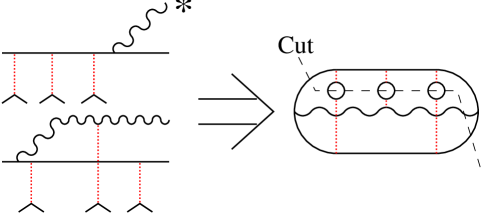
Figure 4: Two processes whose interference is important in determining the gluon bremsstrahlung rate, and the 2PI diagram they imply. Red lines are soft ($gT$) gauge propagators in the Landau cut.

scatterings is shown in Fig. 4. In this and following figures, dotted lines are soft spacelike gauge boson propagators (in the Landau cut), while solid lines are always hard and on-shell; I use wavy rather than curly lines for gluons to make the pictures less cluttered. I have shown the loops responsible for the spectral weight of the soft lines for clarity; all lines in the 2PI formalism are always self-energy resummed. This is one of a family of diagrams which must be included. Any number of soft lines are permitted, provided that they do not cross; so for instance, in the calculation of shear viscosity it is necessary to include 2PI diagrams such as those shown in Fig. 5, just to get leading order results in $g_{\rm s}$.

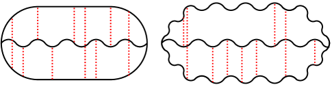
Figure 5: Examples of required diagrams.

If one is willing to make extra approximations, the presence of this infinite class of diagrams need not be fatal. There is a parametric difference between the soft exchange momenta and the hard momenta of the main lines in the diagrams. The soft exchanges can be resummed. This leads to the integral equation for the splitting process already presented in Eq. (5); together with a gradient expansion, this should be the most efficient way to derive the Boltzmann equation presented in the last section. However, for the take-no-prisoners approach, an infinite set of diagrams is a show-stopper. Either some approximation must be made to resum them (and this probably demands some gradient expansion treatment or separation of time scales), the set of diagrams must be truncated, or the numerical approach becomes impossible. Truncating the set of diagrams raises new problems, because it is only the whole set, not any truncation, which is gauge invariant, and even then only when the distinction between $gT$ and $T$ momenta is made parametric. (A truncation also obviously means abandoning a leading order treatment–in fact, even a next to leading log treatment.)

In conclusion, the 2PI formalism looks like a good way to derive the Boltzmann equation. It may provide a good framework for a consistent power counting effort, to prove that the claimed set of diagrams is complete. But as a direct computational tool, it appears ill suited in a gauge theory.

3.2 Diagrammatic approach

The diagrammatic approach to evaluating transport coefficients, in relativistic field theory, was pioneered by Jeon[11]. Recently his (inefficient) treatment has been streamlined[12, 13] and applied, at leading logarithmic order, to gauge theory[13]. Jeon showed that the diagrams which contribute at leading order are ladder diagrams, with a general form shown in Fig. 6.

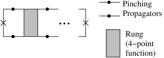
Figure 6: General structure of ladder diagrams. Diagrams with any number of rungs (0,1,2,3,$\ldots$) are needed. The crosses are operator ($T_{\mu\nu}$ or current) insertions.

The self-energy needed on the pinching, nearly on-shell propagators is determined by differentiating the $\Phi$ functional with respect to the propagator once (opening one line), while the rung is obtained by differentiating twice (opening two lines). In scalar field theory, this leads to a relatively tidy set of diagrams. But in a gauge theory, the very complicated 2PI diagrams discussed above lead to a set of diagrams, required at leading order, which is rather intimidating. For instance,

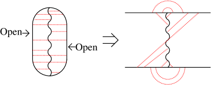
Figure 7: A bubble, which when opened gives a horrible ladder rung.

in Fig. 7 I show the result of opening one of the required 2PI bubble graphs on two of its lines, to get a required ladder rung.

An illustrative example of one of the graphs in the general class which must be resummed, to determine the shear viscosity of QCD with fermions, is shown in Fig. 8.

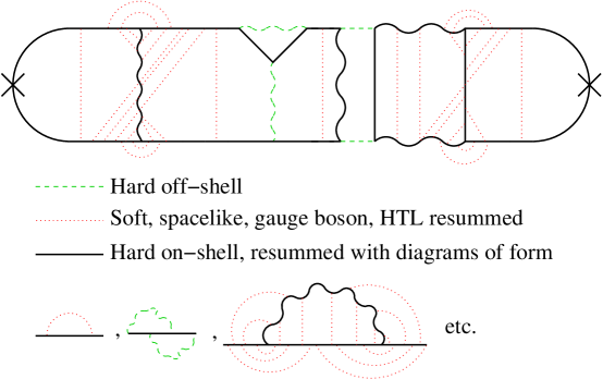
Figure 8: A typical diagram needed in the calculation of leading order shear viscosity in QCD.

This diagram will hopefully give the impression that computing transport at leading order in $g_{\rm s}$, in ultra-relativistic gauge theories, by a direct diagrammatic attack, is pretty hopeless.

4 Conclusions

Don’t get me wrong. I actually quite like the 2PI approach to dynamics. But it is not well suited to gauge theories, except as a method to do a convincing derivation of the Boltzmann equations, which should then be used to solve problems like transport coefficients. Direct numerical application on a lattice, such as has been done in scalar theories[2, 3, 4], is probably hopeless (if complete leading order in $g_{\rm s}$ results are desired–a Boltzmann-Vlasov approach, valid for transport at leading log order, may be feasible and might have some utility).

As for the diagrammatic approach: I defy its supporters to give a convincing power counting argument, without reference either to 2PI or to kinetic theory, that the set of diagrams which I describe above, is both necessary and sufficient. Their resummation is expected to be technically challenging, and in the end it will only boil down to a derivation of the Boltzmann equations. I don’t see the benefit of doing this exercise.

References

- [1] P. Arnold, G. D. Moore and L. G. Yaffe, JHEP 0011, 001 (2000) [hep-ph/0010177].
- [2] J. Berges and J. Cox, Phys. Lett. B 517, 369 (2001) [hep-ph/0006160]; J. Berges, Nucl. Phys. A 699, 847 (2002) [hep-ph/0105311].
- [3] G. Aarts, D. Ahrensmeier, R. Baier, J. Berges and J. Serreau, Phys. Rev. D 66, 045008 (2002) [hep-ph/0201308].
- [4] J. Berges and J. Serreau, hep-ph/0208070.
- [5] P. Arnold, G. D. Moore and L. G. Yaffe, hep-ph/0209353.
- [6] P. Arnold, G. D. Moore and L. G. Yaffe, JHEP 0111, 057 (2001) [hep-ph/0109064].
- [7] P. Arnold, G. D. Moore and L. G. Yaffe, JHEP 0206, 030 (2002) [hep-ph/0204343].
- [8] B. L. Combridge, J. Kripfganz and J. Ranft, Phys. Lett. B70, 234 (1977).
- [9] E. Calzetta and B. L. Hu, Phys. Rev. D 37, 2878 (1988).
- [10] E. A. Calzetta, B. L. Hu and S. A. Ramsey, Phys. Rev. D 61, 125013 (2000) [hep-ph/9910334].
- [11] S. Jeon, Phys. Rev. D 52, 3591 (1995) [hep-ph/9409250].
- [12] E. Wang and U. W. Heinz, Phys. Lett. B 471, 208 (1999) [hep-ph/9910367]; E. Wang and U. W. Heinz, hep-th/0201116.
- [13] M. A. Valle Basagoiti, Phys. Rev. D 66, 045005 (2002) [hep-ph/0204334].