Testing Neutrino Parameters at Future Accelerators

Abstract

The simplest unified extension of the Minimal Supersymmetric Standard Model with bilinear R–Parity violation provides a predictive scheme for neutrino masses which can account for the observed atmospheric and solar neutrino anomalies. Despite the smallness of neutrino masses R-parity violation is observable at present and future high-energy colliders, providing an unambiguous cross-check of the model.

1 Introduction

The announcement of high statistics atmospheric neutrino data by the SuperKamiokande collaboration [1] has confirmed the deficit of muon neutrinos, especially at small zenith angles, opening a new era in neutrino physics. Although there may be alternative solutions of the atmospheric neutrino anomaly  [2] it is fair to say that the simplest interpretation of the data is in terms of $\nu_{\mu}$ to $\nu_{\tau}$ flavor oscillations with maximal mixing. This excludes a large mixing among $\nu_{\tau}$ and $\nu_{e}$ [1], in agreement also with the CHOOZ reactor data [3]. On the other hand the persistent disagreement between solar neutrino data and theoretical expectations [4] has been a long-standing problem in physics. Recent solar neutrino data [5] are consistent with both vacuum oscillations and MSW conversions. In the latter case the large mixing angle solutions are now clearly preferred  [2].

Many attempts have appeared in the literature to explain the data. Here we review recent results [6] obtained in a model [7] which is a simple extension of the MSSM with bilinear R-parity violation (BRpV). This model, despite being a minimal extension of the MSSM, can explain the solar and atmospheric neutrino data. Its most attractive feature is that it gives definite predictions for accelerator physics for the same range of parameters that explain the neutrino data.

2 Bilinear R-Parity Violation

2.1 The Model

Since BRpV SUSY has been discussed in the literature several times [6, 7, 8] we will repeat only the main features of the model here. We will follow the notation of [6]. The simplest bilinear $R_{p}/\;\>$ model (we call it the $R_{p}/\;\>$ MSSM) is characterized by three additional terms in the superpotential

$$W=W_{MSSM}+W_{R\!\!\!/_{P}}$$ (1)

where $W_{MSSM}$ is the ordinary superpotential of the MSSM and

$$W_{R\!\!\!/_{P}}=\epsilon_{i}\widehat{L}_{i}\widehat{H}_{u}.$$ (2)

These bilinear terms, together with the corresponding terms in the soft SUSY breaking part of the Lagrangian,

$${\mathcal{L}}_{soft}={\mathcal{L}}_{soft}^{MSSM}+B_{i}\epsilon_{i}{\tilde{L}}_{i}H_{u}$$ (3)

define the minimal model, which we will adopt throughout this paper. The appearance of the lepton number violating terms in Eq. (3) leads in general to non-zero vacuum expectation values for the scalar neutrinos $\langle{\tilde{\nu}}_{i}\rangle$, called $v_{i}$ in the rest of this paper, in addition to the VEVs $v_{U}$ and $v_{D}$ of the MSSM Higgs fields $H_{u}^{0}$ and $H_{d}^{0}$. Together with the bilinear parameters $\epsilon_{i}$ the $v_{i}$ induce mixing between various particles which in the MSSM are distinguished (only) by lepton number (or R–parity). Mixing between the neutrinos and the neutralinos of the MSSM generates a non-zero mass for one specific linear superposition of the three neutrino flavor states of the model at tree-level while 1-loop corrections provide mass for the remaining two neutrino states, see [6].

3 Neutrino Masses and Mixings

3.1 Tree Level Neutral Fermion Mass Matrix

In the basis $\psi^{0T}=(-i\lambda^{\prime},-i\lambda^{3},\widetilde{H}_{d}^{1},\widetilde{H}_{u}^{2},\nu_{e},\nu_{\mu},\nu_{\tau})$ the neutral fermions mass terms in the Lagrangian are given by

$$\mathcal{L}_{m}=-\frac{1}{2}(\psi^{0})^{T}{\kern-0.24994pt\hbox{$M$}\kern-10.79166pt\kern 0.50003pt\hbox{$M$}\kern-10.79166pt\kern-0.24994pt\raise 0.43304pt\hbox{$M$}}_{N}\psi^{0}+h.c.$$ (4)

where the neutralino/neutrino mass matrix is

$${\kern-0.24994pt\hbox{$M$}\kern-10.79166pt\kern 0.50003pt\hbox{$M$}\kern-10.79166pt\kern-0.24994pt\raise 0.43304pt\hbox{$M$}}_{N}=\left[\begin{array}[]{cc}\mathcal{M}_{\chi^{0}}&m^{T}\cr m&0\cr\end{array}\right]$$ (5)

with

$$\mathcal{M}_{\chi^{0}}=\left[\begin{array}[]{cccc}M_{1}&0&-\frac{1}{2}g^{\prime}v_{d}&\frac{1}{2}g^{\prime}v_{u}\cr 0&M_{2}&\frac{1}{2}gv_{d}&-\frac{1}{2}gv_{u}\cr-\frac{1}{2}g^{\prime}v_{d}&\frac{1}{2}gv_{d}&0&-\mu\cr\frac{1}{2}g^{\prime}v_{u}&-\frac{1}{2}gv_{u}&-\mu&0\cr\end{array}\right]\quad;\quad m=\left[\begin{array}[]{c}a_{1}\cr a_{2}\cr a_{3}\end{array}\right]$$ (6)

where $a_{i}=(-\frac{1}{2}g^{\prime}v_{i},\frac{1}{2}gv_{i},0,\epsilon_{i})$. This neutralino/neutrino mass matrix is diagonalized by

$$\mathcal{N}^{*}{\kern-0.24994pt\hbox{$M$}\kern-10.79166pt\kern 0.50003pt\hbox{$M$}\kern-10.79166pt\kern-0.24994pt\raise 0.43304pt\hbox{$M$}}_{N}\mathcal{N}^{-1}={\rm diag}(m_{\chi^{0}_{1}},m_{\chi^{0}_{2}},m_{\chi^{0}_{3}},m_{\chi^{0}_{4}},m_{\nu_{1}},m_{\nu_{2}},m_{\nu_{3}})$$ (7)

3.2 Approximate Diagonalization at Tree Level

If the $R_{p}/\;\>$ parameters are small, then we can block-diagonalize ${\kern-0.24994pt\hbox{$M$}\kern-10.79166pt\kern 0.50003pt\hbox{$M$}\kern-10.79166pt\kern-0.24994pt\raise 0.43304pt\hbox{$M$}}_{N}$ approximately to the form diag($m_{eff},\mathcal{M}_{\chi^{0}}$)

$$m_{eff}=-m\cdot\mathcal{M}_{\chi^{0}}^{-1}m^{T}=\frac{M_{1}g^{2}+M_{2}{g^{\prime}}^{2}}{4\,det(\mathcal{M}_{\chi^{0}})}\left(\begin{array}[]{ccc}\Lambda_{e}^{2}&\Lambda_{e}\Lambda_{\mu}&\Lambda_{e}\Lambda_{\tau}\\ \Lambda_{e}\Lambda_{\mu}&\Lambda_{\mu}^{2}&\Lambda_{\mu}\Lambda_{\tau}\\ \Lambda_{e}\Lambda_{\tau}&\Lambda_{\mu}\Lambda_{\tau}&\Lambda_{\tau}^{2}\end{array}\right).$$ (8)

The matrices $N$ and $V_{\nu}$ diagonalize $\mathcal{M}_{\chi^{0}}$ and $m_{eff}$

$$N^{*}\mathcal{M}_{\chi^{0}}N^{\dagger}=diag(m_{\chi^{0}_{i}})\quad;\quad V_{\nu}^{T}m_{eff}V_{\nu}=diag(0,0,m_{\nu}),$$ (9)

where

$$m_{\nu}=Tr(m_{eff})=\frac{M_{1}g^{2}+M_{2}{g^{\prime}}^{2}}{4\,det(\mathcal{M}_{\chi^{0}})}|{\vec{\Lambda}}|^{2}.$$ (10)

3.3 Approximate Formulas for 1–Loop

3.3.1 The masses

Looking at the numerical results [6] we found that the most important contribution came from the bottom-sbottom loop. To gain an analytical understanding of the results we expanded the exact results in the small $R\!\!\!\!/_{P}$ parameters. The result is [9]

$$M_{\nu}\simeq c_{0}\left(\matrix{\Lambda_{1}\Lambda_{1}&\Lambda_{1}\Lambda_{2}&\Lambda_{1}\Lambda_{3}\cr\Lambda_{2}\Lambda_{1}&\Lambda_{2}\Lambda_{2}&\Lambda_{2}\Lambda_{3}\cr\Lambda_{3}\Lambda_{1}&\Lambda_{3}\Lambda_{2}&\Lambda_{3}\Lambda_{3}}\right)+c_{1}\left(\matrix{\epsilon_{1}\epsilon_{1}&\epsilon_{1}\epsilon_{2}&\epsilon_{1}\epsilon_{3}\cr\epsilon_{2}\epsilon_{1}&\epsilon_{2}\epsilon_{2}&\epsilon_{2}\epsilon_{3}\cr\epsilon_{3}\epsilon_{1}&\epsilon_{3}\epsilon_{2}&\epsilon_{3}\epsilon_{3}}\right)$$ (11)

where

$$c_{0}=\frac{M_{1}\,g^{2}+M_{2}\,g^{\prime 2}}{4\,\det(M_{\chi^{0}})}\quad;\quad c_{1}=\frac{3}{16\pi^{2}}\,m_{b}\,\sin 2\theta_{b}\,\frac{h^{2}_{b}}{\mu^{2}}\,\log\frac{m^{2}_{\tilde{b_{2}}}}{m^{2}_{\tilde{b_{1}}}}$$ (12)

Diagonalization of the mass matrix gives [9]

$$m_{\nu_{1}} = 0$$ (13)

$$m_{\nu_{2}} \simeq \frac{3}{16\pi^{2}}\,m_{b}\,\sin 2\theta_{b}\,\frac{h^{2}_{b}}{\mu^{2}}\ \log\frac{m^{2}_{\tilde{b_{2}}}}{m^{2}_{\tilde{b_{1}}}}\ \frac{(\vec{\epsilon}\times\vec{\Lambda})^{2}}{|\vec{\Lambda}|^{2}}$$ (14)

$$m_{\nu_{3}} \simeq \frac{M_{1}\,g^{2}+M_{2}\,g^{\prime 2}}{4\,\det(M_{\chi^{0}})}\ |\vec{\Lambda}|^{2}$$ (15)

The formula for $m_{\nu_{3}}$ is the tree-level formula that we used to fix the scale of the atmospheric neutrinos by choosing $|\vec{\Lambda}|$. Details of the derivation can be found in Ref. [9] where the second most important contribution, coming from the loop with charged Higgs/charged leptons, is also discussed.

3.3.2 The mixings

The atmospheric angle is easily obtained in terms of the ratio $\Lambda_{2}/\Lambda_{3}$. For the solar angle in the same approximation we also get a simple formula [9],

$$\tan^{2}\theta_{sol}=\frac{2\epsilon^{2}}{(\epsilon_{2}+\epsilon_{3})^{2}}$$ (16)

that is also in very good agreement with the exact result.

4 Results for the Solar and Atmospheric Neutrinos

4.1 The masses

The BRpV model produces a hierarchical mass spectrum for almost all choices of parameters. The largest mass can be estimated by the tree level value using Eq. (15). Correct $\Delta m^{2}_{atm}$ can be easily obtained by an appropriate choice of $|\vec{\Lambda}|$. The mass scale for the solar neutrinos is generated at 1–loop level and therefore depends in a complicated way in the model parameters. However, in most cases the result of Eq. (14) is a good approximation and there is no problem in having both $\Delta m^{2}_{atm}$ and $\Delta m^{2}_{solar}$ set to the correct scales.

4.2 The mixings

Now we turn to the discussion of the mixing angles. We have found that if $\epsilon^{2}/|\vec{\Lambda}|\ll 100$ then the 1–loop corrections are not larger than the tree level results and the flavor composition of the 3rd mass eigenstate is approximately given by

$$U_{\alpha 3}\approx\Lambda_{\alpha}/|\vec{\Lambda}|$$ (17)

As the atmospheric and reactor neutrino data tell us that $\nu_{\mu}\rightarrow\nu_{\tau}$ oscillations are preferred over $\nu_{\mu}\rightarrow\nu_{e}$, we conclude that

$$\Lambda_{e}\ll\Lambda_{\mu}\simeq\Lambda_{\tau}$$ (18)

are required for BRpV to fit the data. This is sown in Fig. 1 a). We cannot get so easily maximal mixing for solar neutrinos, because in this case $U_{e3}$ would be too large contradicting the CHOOZ result as shown in Fig. 1 b).

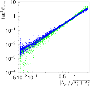
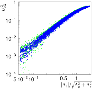
Figure 1: a) Atmospheric angle as a function of $|\Lambda_{\mu}|/\sqrt{\Lambda^{2}_{e}+\Lambda^{2}_{\tau}}$. b) $U^{2}_{e3}$ as a function of $|\Lambda_{e}|/\sqrt{\Lambda^{2}_{\mu}+\Lambda^{2}_{\tau}}$.

We have then two scenarios. In the first one, that we call the mSUGRA case, we have universal boundary conditions of the soft SUSY breaking terms. In this case we can show [6] that

$$\frac{\epsilon_{e}}{\epsilon_{\mu}}\simeq\frac{\Lambda_{e}}{\Lambda_{\mu}}$$ (19)

Then from Fig. 1 b) and the CHOOZ constraint on $U^{2}_{e3}$, we conclude that both ratios in Eq. (19) have to be small. Then from Fig. 2 we conclude that the only possibility is the small angle mixing solution for the solar neutrino problem. In the second scenario, which we call the MSSM case, we consider non–universal boundary conditions of the soft SUSY breaking terms. We have shown that even a very small deviation from universality of the soft parameters at the GUT scale relaxes this constraint. In this case

$$\frac{\epsilon_{e}}{\epsilon_{\mu}}\not=\frac{\Lambda_{e}}{\Lambda_{\mu}}$$ (20)

Then we can have at the same time small $U_{e3}^{2}$ determined by $\Lambda_{e}/\Lambda_{\mu}$ as in Fig. 1 b) and large $\tan^{2}(\theta_{solar})$ determined by $\epsilon_{e}/\epsilon_{\mu}$ as in Fig. 2 b).

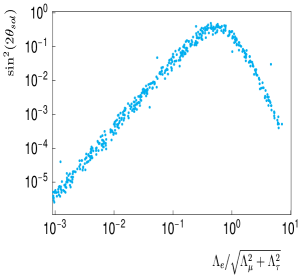
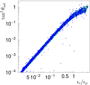
Figure 2: Solar angle as function of: a) $|\Lambda_{e}|/\sqrt{\Lambda^{2}_{\mu}+\Lambda^{2}_{\tau}}$  ; b) $\epsilon_{e}/\epsilon_{\mu}$.

5 Probing Neutrino Mixing via Neutralino Decays

If R-parity is broken, the neutralino is unstable and it will decay through the following channels: $\tilde{\chi}^{0}_{1}\to\nu_{i}\,\nu_{j}\,\nu_{k},\ \nu_{i}\,q\,\bar{q},\ \nu_{i}\,l^{+}_{j}\,l^{-}_{k},\ l^{\pm}_{i}\,q\,\bar{q}^{\prime},\ \nu_{i}\,\gamma$. It was shown in Ref. [10], that the neutralino decays well inside the detectors and that the visible decay channels are quite large. This was fully discussed in Ref. [10] where it was shown that the ratios $|\Lambda_{i}/\Lambda_{j}|$ and $|\epsilon_{i}/\epsilon_{j}|$ were very important in the choice of solutions for the neutrino mixing angles. What is exciting now, is that these ratios can be measured in accelerator experiments. In the left panel of Fig. 3 we show the ratio of branching ratios for semileptonic LSP decays into muons and taus: $BR(\chi\to\mu q^{\prime}\bar{q})/BR(\chi\to\tau q^{\prime}\bar{q}$) as function of $\tan^{2}\theta_{atm}$. We can see that there is a strong correlation. The spread in this figure can in fact be explained by the fact that we do not know the SUSY parameters. This is illustrated in the right panel where we considered that SUSY was already discovered with the following values for the parameters,

$$M_{2}=120\,GeV,\mu=500\,GeV,\tan\beta=5,m_{0}=500\,GeV,A=-500\,GeV$$ (21)

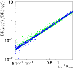
Figure 3: Ratios of semileptonic branching ratios as functions of $\tan\theta_{atm}$. On the left for random SUSY values and on the right for the SUSY point of Eq. (21)

6 Probing Neutrino Mixing via Charged Lepton Decays

If R-parity is broken the lightest supersymmetric particle (LSP) will decay. If the LSP decays then cosmological and astrophysical constraints on its nature no longer apply. Thus, within R-parity violating SUSY a priori any superparticle could be the LSP. We have studied [12] the case where a charged scalar lepton, most probably the scalar tau, is the LSP. The production and decays of ${\tilde{\tau}}$, as well as the decays of ${\tilde{e}}$ and ${\tilde{\mu}}$, and demonstrate that also for the case of charged sleptons as LSPs neutrino physics leads to definite predictions of various decay properties. This is shown in Figs. 4 and 5

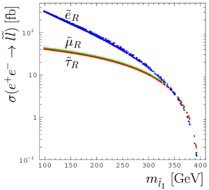
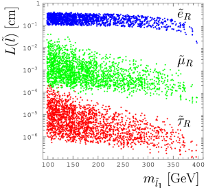
Figure 4: a)$e^{+}e^{-}\to{\tilde{l}}{\tilde{l}}$ production cross section at a Linear Collider $\sqrt{s}=0.8\hbox{TeV}$, b) Charged slepton decay length at a linear collider with $\sqrt{s}=0.8\hbox{TeV}$.

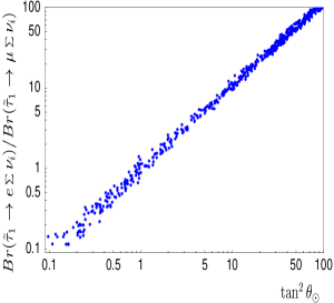
Figure 5: Ratios of branching ratios for scalar tau decays versus $\tan^{2}\theta_{\odot}$. The left panel shown all data points, the right one refers only to data points with $\epsilon_{2}/\epsilon_{3}$ restricted to the range [0.9,1.1].

7 Conclusions

The Bilinear R-Parity Violation Model is a simple extension of the MSSM that leads to a very rich phenomenology. We have calculated the one–loop corrected masses and mixings for the neutrinos in a completely consistent way, including the RG equations and correctly minimizing the potential. We have shown that it is possible to get easily maximal mixing for the atmospheric neutrinos and both small and large angle MSW.

We emphasize that the LSP decays inside the detectors, thus leading to a very different phenomenology than the MSSM. The LSP can be either the lightest neutralino, like in the MSSM, or a charged particle, must probably the lightest stau. In both cases we have shown that ratios of the branching ratios of the LSP can be correlated with the neutrino parameters.

If the model is to explain solar and atmospheric neutrino problems many signals will arise at future colliders. These will probe the neutrino mixing parameters. Thus the model is easily falsifiable!

References

- [1] S. Fukuda et al. [Super-Kamiokande Collaboration], of Super-Kamiokande-I data,” Phys. Lett. B 539 (2002) 179 [arXiv:hep-ex/0205075]. Phys. Rev. Lett. 81, 1562 (1998) [arXiv:hep-ex/9807003].
- [2] M. Maltoni, T. Schwetz, M. A. Tortola and J. W. Valle, atmospheric data,” arXiv:hep-ph/0207227, Phys. Rev. D in press; M. C. Gonzalez-Garcia, M. Maltoni, C. Pena-Garay and J. W. F. Valle, Phys. Rev. D 63 (2001) 033005 [hep-ph/0009350];
- [3] M. Apollonio et al, CHOOZ Coll., Phys. Lett. B 466 (1999) 415; F. Boehm et al, Palo Verde Coll., Phys. Rev. D 64 (2001) 112001
- [4] J. N. Bahcall, S. Basu and M. H. Pinsonneault, Phys. Lett. B 433, (1998) 1.
- [5] Q. R. Ahmad et al. [SNO Collaboration], constraints on neutrino mixing parameters,” Phys. Rev. Lett. 89 (2002) 011302 [arXiv:nucl-ex/0204009].
- [6] J. C. Romão, M. A. Diaz, M. Hirsch, W. Porod and J. W. Valle, Phys. Rev. D 61, 071703 (2000) [arXiv:hep-ph/9907499]; M. Hirsch, M. A. Diaz, W. Porod, J. C. Romão and J. W. Valle, Phys. Rev. D 62, 113008 (2000) [Erratum-ibid. D 65, 119901 (2002)] [arXiv:hep-ph/0004115].
- [7] M. A. Diaz, J. C. Romão and J. W. Valle, Nucl. Phys. B 524, 23 (1998) [arXiv:hep-ph/9706315].
- [8] F. de Campos, M. A. Garcia-Jareno, A. S. Joshipura, J. Rosiek and J. W. Valle, Nucl. Phys. B 451 (1995) 3 [arXiv:hep-ph/9502237]. A. G. Akeroyd, M. A. Diaz, J. Ferrandis, M. A. Garcia-Jareno and J. W. Valle, Nucl. Phys. B 529, 3 (1998) [arXiv:hep-ph/9707395]. T. Banks, Y. Grossman, E. Nardi and Y. Nir, Phys. Rev. D 52, 5319 (1995) [arXiv:hep-ph/9505248].
- [9] M. Hirsch, M. A. Diáz, W. Porod, J. W. F. Valle and J. C. Romão, work in preparation.
- [10] W. Porod, M. Hirsch, J. Romão and J. W. Valle, Phys. Rev. D63 (2001) 115004, [arXiv:hep-ph/0011248].
- [11] B. Mukhopadhyaya, S. Roy and F. Vissani, Phys. Lett. B 443 (1998) 191, [arXiv:hep-ph/9808265].
- [12] M. Hirsch, W. Porod, J. C. Romão and J. W. Valle, Phys. Rev. D. in press, [arXiv:hep-ph/0207334].