Testing the solar LMA region with KamLAND data

Abstract

We investigate the potential of 3 kiloTon-years(kTy) of KamLAND data to further constrain the $\Delta m^{2}$ and $\tan^{2}\theta$ values compared to those presently allowed by existing KamLAND and global solar data. We study the extent, dependence and characteristics of this sensitivity in and around the two parts of the LMA region that are currently allowed. Our analysis with 3 kTy simulated spectra shows that KamLAND spectrum data by itself can constrain $\Delta m^{2}$ with high precision. Combining the spectrum with global solar data further tightens the constraints on allowed values of $\tan^{2}\theta$ and $\Delta m^{2}$. We also study the effects of future neutral current data with a total error of 7% from the Sudbury Neutrino Observatory. We find that these future measurements offer the potential of considerable precision in determining the oscillation parameters (specially the mass parameter).

1 Introduction

The Sudbury Neutrino Observatory (SNO) charged current (CC) and neutral current (NC) data on the measurement of solar neutrino flux has provided strong evidence for neutrino flavor conversion [1, 2] and it establishes the presence of $\nu_{\mu}/\nu_{\tau}$ flavor in the solar $\nu_{e}$ flux at 5.5$\sigma$ level. The SNO and SK results together with the data from the radiochemical experiments Cl [3] and Ga [4] single out the LMA solution based on MSW resonant matter conversion as the most probable solution of the solar neutrino puzzle [7]-[17]. In [9], for instance, this solution is characterized by best fit values of $\tan^{2}\theta=0.41,\Delta m^{2}=6.06\times 10^{-5}$eV² for the neutrino mixing parameters. Spectacular confirmation in favour of this solution, using terrestrial neutrino sources, has come recently from the KamLAND experiment in Japan [18]. The uniqueness of KamLAND [19, 20, 21] lies in its sensitivity to masses lying in the LMA region through its measurement of the reactor antineutrino energy spectrum. With 162 ton-years of data, KamLAND has already split the allowed LMA zone into two smaller sub-zones, the low-LMA with $\mbox{$\Delta{m}^{2}$~{}}\sim 7.2\times 10^{-5}$ eV² and the high-LMA zone with $\mbox{$\Delta{m}^{2}$~{}}\sim 1.5\times 10^{-5}$ eV² [22, 23].

In this paper, we consider a broader time-frame than spanned by the first results, and obtain projected results and conclusions that should be forthcoming from a 3 kTy exposure. With present fiducial volume this correspods to KL run of 8 - 10 years time. First we discuss the present constraints and next we discuss the future perspectives in the light of the present data. We determine the allowed areas in the $\Delta m^{2}$-$\tan^{2}\theta$ plane from the analysis of total KamLAND rate, KamLAND spectrum and examine the role of both of these in constraining the allowed regions by themselves as well as in conjunction with the global solar data. We simulate the projected KamLAND spectrum at several sample $\Delta m^{2}$ and $\tan^{2}\theta$ values, taken from the currently allowed regions, and attempt to delineate in detail the limits of sensitivity for KamLAND over a 3 kTy period. We study the dependence of the reconstituted parameter regions on the sample values of $\Delta m^{2}$ and $\tan^{2}\theta$ chosen and demonstrate that for spectrum simulated at points inside both the low-LMA and the high-LMA region the accuracy of reconstruction is quite high, leading to an excellent precision in determination of the oscillation parameters, especially $\Delta m^{2}$.

Section 2 describes the salient features of the KamLAND detector, and the expected ${\bar{\nu_{e}}}$ reactor flux to which it is sensitive. In Section 3 we discuss the analysis procedure and results. Section 4 summarises our conclusions.

2 The KamLAND detector, the reactor flux of Electron Anti-Neutrinos and the Event Rate

KamLAND [19] is a 1 kton liquid scintillator neutrino detector located at the earlier Kamiokande site in the Kamioka mine in Japan. It measures the $\bar{\nu}_{e}$ flux from 16 Japanese nuclear power reactors whose distances range from $80$ km to $800$ km. However $\approx 79\%$ of the measured flux come from reactors situated at distances between 138 km to 214 km from the detector. The reaction that detects the $\bar{{\nu_{e}}}$ is the inverse beta decay $\bar{\nu}_{e}+p\rightarrow e^{+}+n$. The positrons are annihilated to produce two $\gamma$ rays. Neutron capture in the medium also generates a delayed $\gamma$ signal. The correlation between these two records an event grossly free from the backgrounds.

The neutrino spectrum from the fission of a particular isotope $j$ is conveniently parameterizable [21, 24] (in units of MeV^-1 per fission) as

$$dN_{\nu}^{j}/dE_{\nu}=\exp(a_{0}+a_{1}E_{\nu}+a_{2}E_{\nu}^{2}).$$ (1)

Here $j=1,2,3,4$, corresponding to the 4 isotopes ²³⁵U, ²³⁹P, ²³⁸U, ²⁴¹Pu which constitute the fuel. The fitted values of the $a_{k}s$ in the equation above are reproduced for completeness from [21, 24] in Table 1.

Table 1: Fitted Parameters $a_{k},k=0,1,2$ for the reactor neutrino spectrum. The last row shows the energy released for each isotope per fission.

Isotope	235U	239Pu	238U	241Pu
$a_{0}$	0.870	0.896	0.976	0.793
$a_{1}$	-0.160	-0.239	-0.162	-0.080
$a_{2}$	-0.0910	-0.0981	-0.0790	-0.1085
$\epsilon_{j}$ (MeV)	201.7	205.0	210.0	212.4

In addition, each isotope has a characteristic energy released per fission, $\epsilon_{j}$. These are also reproduced from [24] in Table 1.

Table 2 (from [19]) gives the distances of the various reactors from the Kamioka mine which houses KamLAND, along with the maximum thermal power $N^{i}_{max}$ (in Giga-watts) of each $i$, the reactor index, which runs from $1-16$. Also, we note that in principle, the power of each reactor varies over the year depending on demand, fuel composition, re-fuelling times etc. This dependence is averaged over for our purposes, and we assume that each reactor is in the running mode at maximum output 80% of the time.

Table 2: Reactor distances and power outputs

Reactor Site	Distance $d_{i}$ (km)	Power $N_{max}^{i}$(Giga-watts)
Kashiwazaki	160	24.6
Ohi	180	13.7
Takahama	191	10.2
Hamaoka	213	10.6
Tsuruga	139	4.5
Shiga	88	1.6
Mihama	145	4.9
Fukushima-1	344	14.2
Fukushima-2	344	13.2
Tokai-II	295	3.3
Shimane	414	3.8
Ikata	561	6.0
Genkai	755	6.7
Onagawa	430	4.1
Tomari	784	3.3
Sendai	824	5.3

Using the above data, one may then write an expression for the spectrum from a given reactor $i$ as,

$$S_{i}=\sum_{j}\frac{f_{j}^{i}N_{max}^{i}(0.8)}{\sum_{k}f_{k}^{i}\epsilon_{k}}dN_{\nu}^{j}/dE_{\nu}$$ (2)

Here $f_{j}^{i}$ is the fractional abundance of isotope $j$ in reactor $i$ at a given time. The time dependence is again averaged over, and for all the reactors we use for the abundance the values, 53.8% for ²³⁵U, 32.8% for ²³⁹Pu, 7.8% for ²³⁸U, and 5.6% for ²⁴¹Pu, as in [18]. Convenient units for $S_{i}$ are MeV^-1sec^-1, obtained by converting the power in Giga-watts into Mev per sec by multiplying by the factor $6.24\times 10^{21}$.

The other quantities needed to determine the event rate are the cross-section, the survival probability for anti-neutrinos and the number of free proton targets in the scintillator. The cross-section is given by

$$\sigma(E_{\nu})=\frac{2\pi^{2}}{m_{e}^{5}f\tau_{n}}p_{e^{+}}E_{e^{+}}.$$ (3)

Here $f=1.69$ is the integrated Fermi function for neutron $\beta$-decay, $m_{e}$ is the positron mass, $E_{e^{+}}$ is the positron energy, $p_{e^{+}}$ is the positron momentum and $\tau_{n}=886.7$ secs is the neutron lifetime. The total visible energy ($E_{vis}$) corresponds to $E_{e^{+}}+m_{e}$, where $E_{e^{+}}$ is the total energy of the positron and $m_{e}$ the electron mass. The total positron energy is related to the incoming antineutrino energy $E_{\nu}$ through the relation, $E_{e^{+}}=E_{\nu}-(m_{n}-m_{p})-{\bar{E}_{rec}}$, where $m_{n}-m_{p}=1.293$ MeV is the neutron–proton mass difference and ${\bar{E}_{rec}}$ is the average neutron recoil energy calculated here using [25].

The two-generation survival probability for the antineutrinos from each of the reactors $i$ is given by

$$P_{i}(\bar{\nu}_{e}\leftrightarrow\bar{\nu}_{e}) = 1-\sin^{2}2\theta\sin^{2}\left(\frac{1.27\Delta m^{2}d_{i}}{E_{\nu}}\right)$$ (4)

where $d_{i}$ is the distance of reactor $i$ to KamLAND in $km$, $E_{\nu}$ is in GeV and $\Delta m^{2}$ is in eV². Thus the total observed event-rate in KamLAND is given by $N_{KL}$ in sec^-1,

$$N_{KL} = \eta N_{p}\times\int dE_{vis}\int dE_{e^{+}}R(E_{vis},E_{e^{+}})\times$$ (5)

$$\sigma(E_{e^{+}}+1.293)\sum_{i}S_{i}\frac{P_{i}(\bar{\nu}_{e}\leftrightarrow\bar{\nu}_{e})}{4\pi d_{i}^{2}}$$

where $N_{p}$ is the number of free protons in the fiducial volume of the detector. KamLAND has declared 162 ton-year data corresponding to 408 tons fiducial mass containing 3.46$\times 10^{31}$ free protons. The integrated total power $P/{4\pi L^{2}}$ is 254 ${\rm Joule/cm^{2}}$. The efficiency ($\eta$) is 78.3%. R(E_vis,E${}_{e^{+}}$) is the energy resolution function given by

$$R(E_{vis},E_{e^{+}}) = \frac{1}{\sqrt{2\pi\sigma_{0}^{2}}}\exp\left(-\frac{(E_{vis}-E_{e^{+}}-m_{e})^{2}}{2\sigma_{0}^{2}}\right)$$

with $\sigma_{0}$/E${}_{e^{+}}$ = 7.5%/$\sqrt{E_{e^{+}}}$ ($E$ in MeV) [18, 26].

The ratio of the observed event-rate to the expected rate in KamLAND is defined as

$$R_{KL}=\frac{N_{KL}}{N^{0}_{KL}}$$ (6)

where $N^{0}_{KL}$ is the expected event-rate in KamLAND given by Eq.(5) with $P(\bar{\nu}_{e}\leftrightarrow\bar{\nu}_{e})=1$. The first KamLAND results report a $R_{Kl}=0.611\pm 0.085\pm 0.041$ [18].

3 Analysis and Results

3.1 Current Data

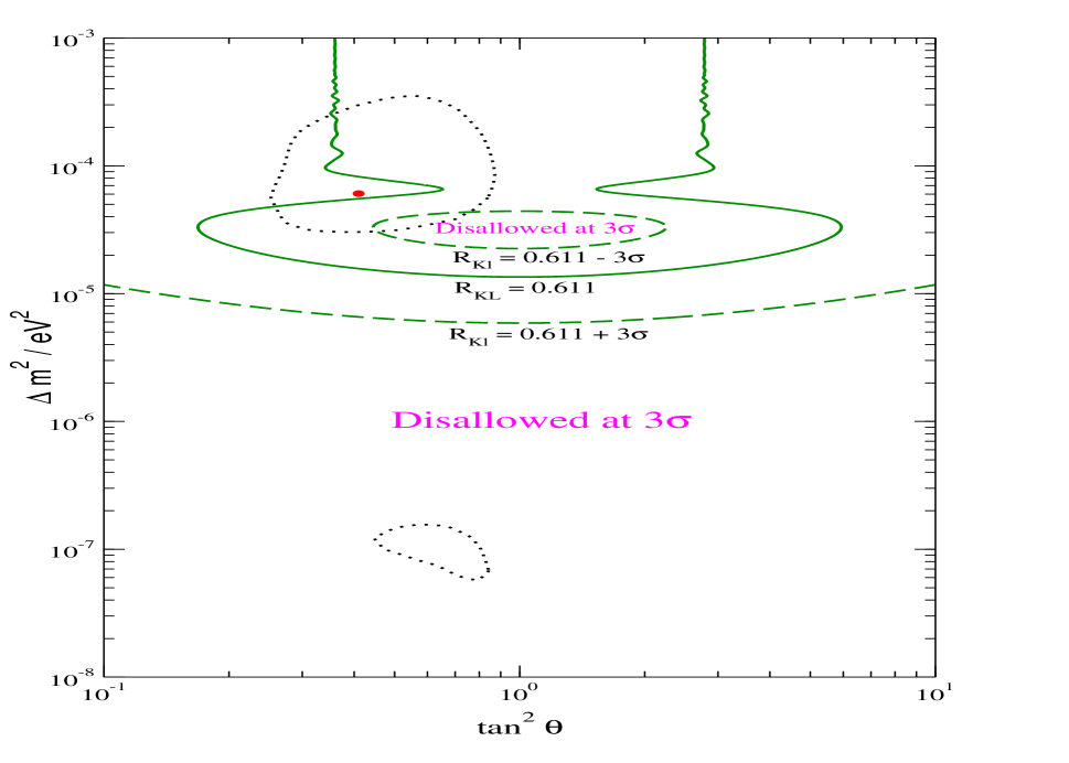
Figure 1: The isorate lines for the KamLAND detector corresponding to the observed rate and $\pm 3\sigma$ limits in the $\Delta m^{2}-\tan^{2}\theta$ plane. Also shown by dotted line is the $3\sigma$ allowed area from the global analysis of the solar neutrino data . The best-fit solution for the solar data is marked.

In Figure 1 we show the lines of constant KamLAND rate $R_{KL}$ in the $\Delta m^{2}-\tan^{2}\theta$ plane for the observed value of 0.611 and $\pm$ 3$\sigma$ limits. The best-fit point from global solar neutrino analysis and the corresponding $3\sigma$ contour (dashed lines) in the LMA and LOW regions are also shown. The best-fit point [8, 9] of the global solar neutrino data predicts a KamLAND rate of 0.65 very close to the observed rate. We note that a particular observed $R_{KL}$ may correspond to a wide range of KamLAND spectra. The reverse, of course, is not true since an observed KamLAND spectrum singles out a unique rate (within errors).

We first do a statistical analysis with the KamLAND rate alone. For the rate we define the $\chi^{2}$ as

$$\chi^{2}_{KL}=\frac{(R_{KL}^{expt}-R_{KL}^{theory})^{2}}{\sigma^{2}}$$ (7)

where $\sigma=\sqrt{\sigma_{syst}^{2}+\sigma_{stat}^{2}}$, $\sigma_{syst}$ and $\sigma_{stat}$ being the total systematic and statistical error in the KamLAND data respectively. We take 6.42% systematic uncertainty along with the published statistical errors. To eliminate the geophysical background we take a visible energy threshold of 2.6 MeV. [18, 26].

For a more complete statistical study, we next do a combined analysis of global solar data and the observed KamLAND rate. We use a combined $\chi^{2}$ function defined as

$$\chi^{2}=\chi^{2}_{\odot}+\chi^{2}_{KL}$$ (8)

For the $\chi^{2}_{\odot}$ (solar), we use the data on total rate from the Cl experiment, the combined rate from the Ga experiments (SAGE+GALLEX+GNO), the 1496 day data on the SK zenith angle energy spectrum and the combined SNO day-night spectrum. We define the $\chi^{2}$ function in the “covariance” approach as

$$\chi^{2}_{\odot}=\sum_{i,j=1}^{N}(R_{i}^{\rm expt}-R_{i}^{\rm theory})(\sigma_{ij}^{2})^{-1}(R_{j}^{\rm expt}-R_{j}^{\rm theory})$$ (9)

where $R_{i}$ are the solar data points, $N$ is the number of data points (80 in our case) and $(\sigma_{ij}^{2})^{-1}$ is the inverse of the covariance matrix, containing the squares of the correlated and uncorrelated experimental and theoretical errors. For further details of our solar analysis we refer the reader to [9, 10].

Figure 2: The 90%, 95%, 99% and 99.73% C.L. contours in the LMA region. The left hand panel gives the allowed region from an analysis of only KamLAND rate. The right hand panel gives the allowed region from a combined solar+KamLAND rate analysis. The purple dashed line shows the $3\sigma$ only solar contour.

In Figure 2 we draw the 90%, 95%, 99% and 99.73% C.L. allowed area in the LMA region from only KamLAND rate and combined solar+KamLAND rate analysis. Superimposed on that we show the $3\sigma$ allowed area from solar data alone. The current observed KamLAND rate is in excellent agreement with the predicted KamLAND rate from the best-fit solution to the solar data. From the left-hand panel of Figure 2 we see that the allowed areas from KamLAND rate data are mostly consistent with the $3\sigma$ allowed area from the global solar data, except from a small region around the bottom right-hand edge of the latter. This fact is again reflected in the global solar and KamLAND rate allowed areas shown in the right-hand panel. The inclusion of the KamLAND rate into the global analysis allows most of the regions allowed before, except for a small region around low $\Delta{m}^{2}$ and large $\tan^{2}\theta$ (the bottom right zone).

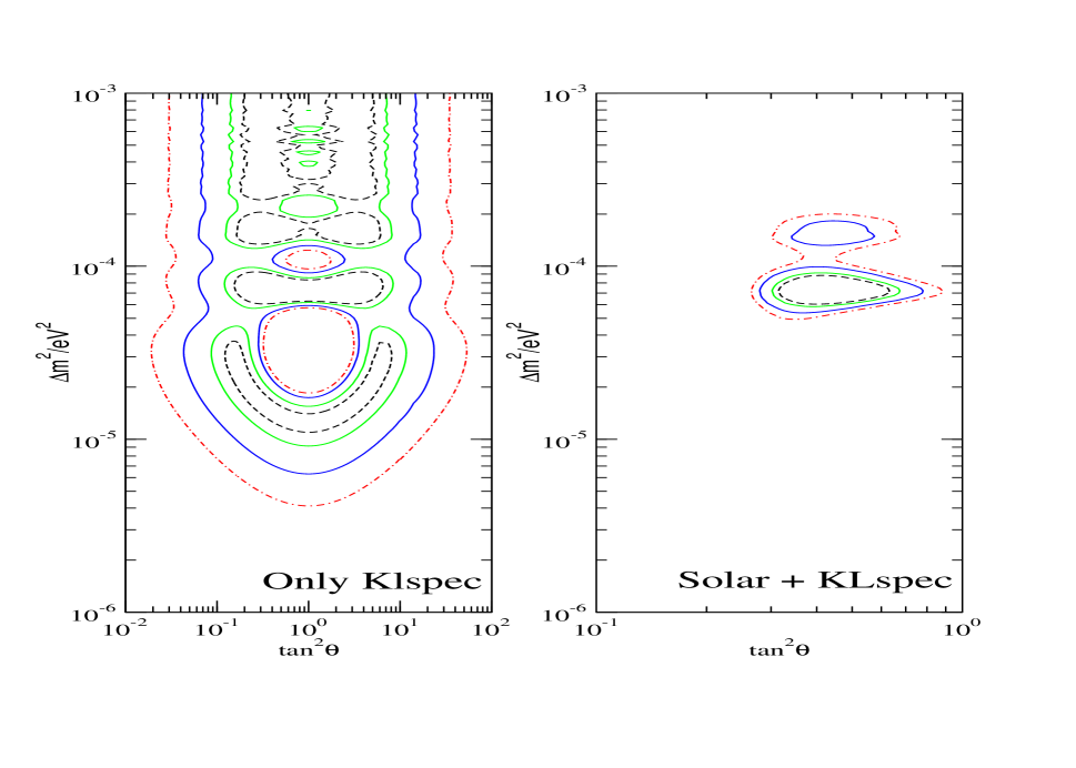
Figure 3: The 90%, 95%, 99% and 99.73% C.L. contours in the LMA region. The left hand panel gives the allowed region from an analysis of only KamLAND spectrum data. The right hand panel gives the allowed region from a combined solar+KamLAND spectrum analysis.

Next, our aim is to see how far the allowed areas can be constrained with the inclusion of KamLAND spectrum data. The current KamLAND spectrum data are rather low on statistics and hence we consider a Poisson distribution for the spectral events. Thus the $\chi^{2}$ for the current KamLAND spectrum is defined as

$$\chi^{2}_{KLspec}=\sum_{i}\left[2(X_{n}N_{i}^{th}-N_{i}^{exp})+2N_{i}^{exp}ln(\frac{N_{i}^{exp}}{X_{n}N_{i}^{th}})\right]+\frac{(X_{n}-1)^{2}}{\sigma^{2}_{sys}}$$ (10)

where $\sigma_{sys}$ is taken to be 6.42%, $X_{n}$ is a normalization allowed to vary freely, and the sum is over the KamLAND spectral bins.

The left hand panel in Figure 3 shows the allowed area from only KamLAND spectrum analysis. The right hand panel in Figure 3 gives the allowed region in the oscillation parameter space after including the global solar data. These contours are obtained by minimising

$$\chi^{2}=\chi^{2}_{\odot}+\chi^{2}_{KLspec}$$ (11)

Together the KamLAND and solar data are instrumental in narrowing down the parameter range by a large amount. At 99% C.L. the allowed LMA region is bifurcated into two parts – a low-LMA zone around the best-fit point $\mbox{$\Delta{m}^{2}$~{}}=7.17\times 10^{-5}$ eV² and $\tan^{2}\theta_{12}=0.44$ and a high-LMA zone around a second best-fit of $\mbox{$\Delta{m}^{2}$~{}}=1.49\times 10^{-4}$ eV² and $\tan^{2}\theta_{12}=0.43$. At 3$\sigma$ the two regions merge.

3.2 3 kton year data

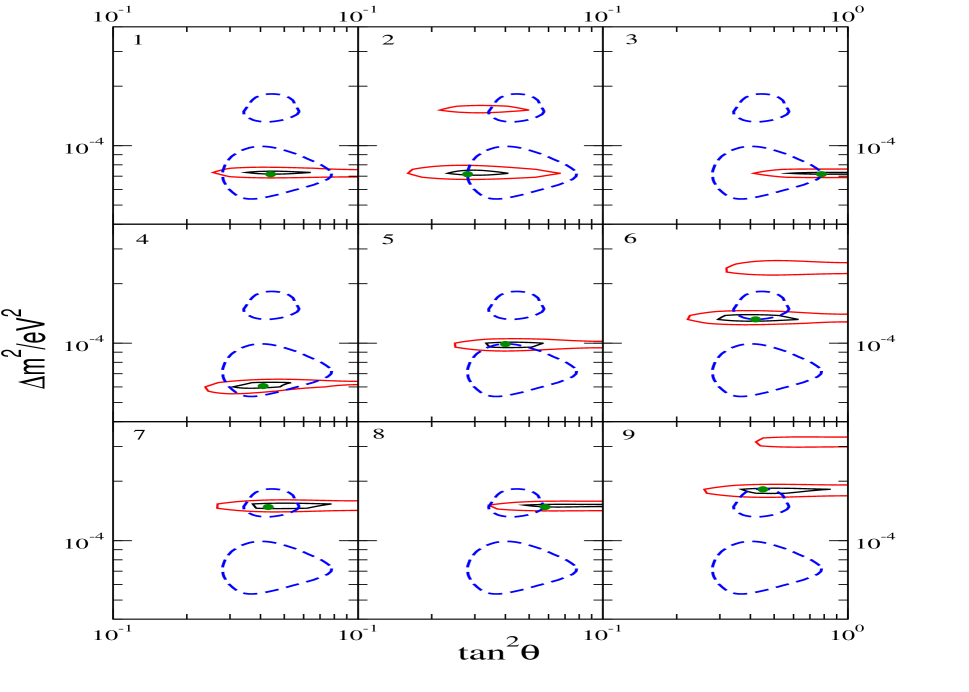
Figure 4: The 1$\sigma$ and 3$\sigma$ contours for the 3 kTy projected KamLAND spectrum analysis alone. The different panels are for the simulated spectrum at different fixed values of $\Delta m^{2}$ and $\tan^{2}\theta$ shown by bold dots. For reference we also show by dashed lines the current 99% C.L. allowed areas from the global analysis of the solar and KamLAND data.

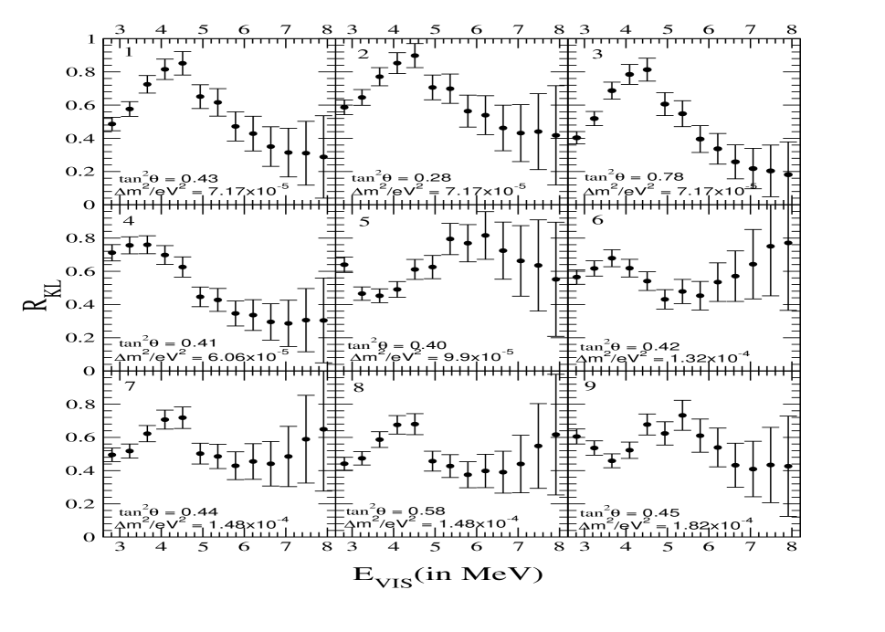
Figure 5: Ratio of oscillated to unoscillated events for the 3kTy simulated KamLAND spectrum for the different sets of $\Delta m^{2}$ and $\tan^{2}\theta$ corresponding to Figure 4.

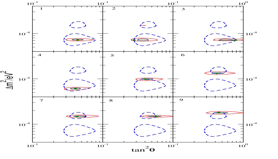
Figure 6: The 1$\sigma$ and 3$\sigma$ contours for the combined analysis including the global solar data, the projected 3 kTy KamLAND data and the CHOOZ reactor data [27]. The different panels are for the simulated spectrum at values of $\Delta m^{2}$ and $\tan^{2}\theta$ of the corresponding panels of Figures 4 and 5. The dashed line shows the presently allowed $3\sigma$ contour from solar+KamLAND spectrum analysis.

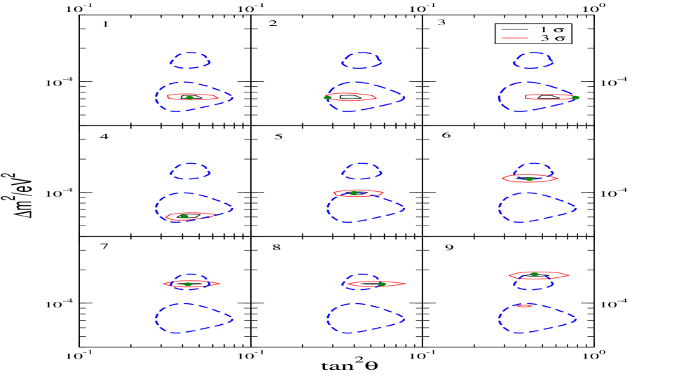
Figure 7: Same as in Figure 6 but with a smaller future projected total uncertainty in the SNO NC rate of only 7%.

In this section we investigate the evolution of the allowed zones as KamLAND collects more statistics for its spectrum data. We do a projected analysis with 3 kTyr KamLAND spectrum simulated at few representative values of $\Delta m^{2}$ and $\tan^{2}\theta$. We randomize the generated spectra to take into account the possible fluctuations. We use these simulated spectra in a $\chi^{2}$ analysis and reconstruct the allowed regions in the $\Delta m^{2}$–$\tan^{2}\theta$ parameter space. Since statistics are expected to be large for the 3 kTy exposure, we consider a Gaussian distribution for the spectral events in this case and define our $\chi^{2}$ function as,

$$\chi^{2}_{KLspec}=\sum_{i,j}(N_{i}^{exp}-N_{i}^{th})(\sigma_{ij}^{2})_{KL}^{-1}(N_{j}^{exp}-N_{j}^{th})$$ (12)

where $(\sigma_{ij}^{2})_{KL}$ is the error correlation matrix, containing the statistical and systematic errors, where the systematic errors are assumed to be fully correlated among the energy bins. For the data we assume the same threshold of 2.6 MeV and the same energy binning as the present data. However the current KamLAND data quotes a conservative value of 6.42% for the systematic uncertainty. In the 3 kton year time span the systematic uncertainty is expected to reduce. The fiducial volume uncertainty which contributes the most at present can go down after the collaboration installs a calibration arm. The cut systematics and energy reconstruction error can also reduce . Keeping this in mind for 3 kTy data we use a optimistic assessment of 3% for the KamLAND systematic error, though we have checked that increasing the systematic uncertainty to 4% (which is the projected value quoted by the KamLAND collaboration) does not change the final conclusions.

Figure 4 shows the reconstituted C.L. allowed contours (1$\sigma$ and 3 $\sigma$) in parameter space from a $\chi^{2}$ analysis using the simulated KamLAND spectrum alone. Marked by black dots are the points at which the spectra have been simulated. Each panel in this set of plots serves to identify regions in the presently allowed LMA region and demonstrates the constraining capabilities of the future KamLAND spectral data. Panels 1-5 are for spectrum simulated in the low-LMA zone while panels 6-9 are for spectrum simulated in the high-LMA zone. For the first three panels the spectrum is simulated at a $\Delta{m}^{2}$ corresponding to the low-LMA best-fit and three different $\theta$s. A comparison of the allowed regions in these three panels show that tighter constraints on $\Delta m^{2}$ and $\tan^{2}\theta$ are associated with higher values of $\tan^{2}\theta$. For most of the cases where $\Delta{m}^{2}$ lies in the low-LMA region, the high-LMA can be ruled out at the $3\sigma$ level. However for the panel 2 which corresponds to the lowest $\theta$ a small region still remains allowed at 3$\sigma$. The panel 4 is for the spectrum simulated at the best-fit solar point, $\Delta m^{2}=6.06\times 10^{-5}$ eV² and $\tan^{2}\theta=0.41$. As we move our simulation point in the high-LMA region in panel 6, a higher $\Delta{m}^{2}$ region becomes allowed. No such region is obtained for the current best-fit point in the high-LMA region in panel 7 as well as panel 8. Note that panel 8 is for the high-LMA best-fit $\Delta{m}^{2}$ but at an increased $\theta$. Again in panel 9 we get some allowed regions at 3$\sigma$ at a high $\Delta{m}^{2}$ . We stress that since the relevant probability for KamLAND is the vacuum oscillation probability each of these panels will admit the mirror solution corresponding to $\theta\rightarrow\pi/2-\theta$, the so called dark zone, which we have not shown explicitly in this figure. However we note that while very tight constraints are obtained for $\Delta{m}^{2}$ , the range of allowed values for $\tan^{2}\theta$ seems to be quite large in general for all the cases. In fact for all but panel 2, we see that maximal mixing is allowed atleast at the $3\sigma$ level, if not better.

Figure 5 shows the distorsions in the simulated spectrum with $\pm 1\sigma$ error bars at the $\Delta m^{2}$ and $\tan^{2}\theta$ corresponding to each of the panels of figure 4. The spectra in panels 6 and 9 of Figure 5 are simulated at a higher value of $\Delta{m}^{2}$ and hence this leads to faster oscillations as compared to the other panels, resulting in a degenerate solution appearing at a higher value of $\Delta{m}^{2}$ in figure 4.

In figure 6 we show the C.L. allowed regions from a combined analysis of the global solar and the 3 kTy KamLAND simulated spectrum data. The KamLAND spectra are simulated at the same points as in Figure 4 and 5. Also superimposed is the 99% C.L. combined solar + present KL contour. If we compare Figure 6 to Figure 4, we note that the contours get more constricted and the higher $\Delta{m}^{2}$ regions appearing in panels 2, 6 and 9 disappear. Inclusion of global solar data also restricts the allowed range in $\tan^{2}\theta$. The maximal mixing solution and the dark zone allowed by the KamLAND spectrum data get disfavoured with the inclusion of solar data in most of the panels, as the SNO data disfavours the maximal mixing solution. However for panels 3 and 8 for which the simulation point is at a larger $\theta$ the maximal mixing solution continues to be allowed at $3\sigma$, as these points correspond to spectra for which the KamLAND contribution to $\chi^{2}$ is much less at maximal mixing.

In figure 7 we study the effect of reducing the SNO NC error in the analysis with 3 kTy KamLAND spectrum data. The current SNO NC data is due to neutron capture on deuteron the efficiency for which is 30%. SNO has added NaCl in the detector which has the effect of enhancing the neutron capture efficiency to 83%. With this the statistical error in SNO NC measurements is expected to reduce to about 5% [29]. The SNO collaboration are also improving their systematics. They expect to have less than 3% systematic uncertainty on neutron capture and would also reduce the uncertainties in their energy scale and energy resolution [29]. Keeping this in mind we assume an optimistic reduction in the current systematic error of 9% and we use a total SNO NC error of 7% [30] in place of the current 12% in figure 7. We do a $\chi^{2}$-analysis of global solar data and the simulated KamLAND spectrum data. In plotting this figure, we use the total charged current and neutral current rates instead of the SNO spectrum data which implicitly assumes absence of spectral distortion for the resultant ${}^{8}B$ flux at SNO. Since we are in the LMA region we consider this to be a justified approximation above the SNO threshold of 5 MeV. This figure is a most optimistic projection of how far the allowed ranges of $\Delta{m}^{2}$ and $\tan^{2}\theta$ can be constrained in the future. We find that the reduction of the SNO NC error reduces the allowed range of $\theta$ as compared to that in figure 6. In particular in the panels 3,8 and 9 maximal mixing were allowed with 3 kTy KamLAND data but reducing the SNO NC error disfavours maximal mixing in these panels.

In Table 3 we summarise the allowed ranges in $\Delta{m}^{2}$ and $\tan^{2}\theta$ as obtained from analysis with solar + 3 kTy KamLAND spectrum data and solar (with sno NC 7%) and 3 kTy KamLAND spectrum data. Note that for 3 kTy KamLAND spectrum we use an optimistic value of 3% for the KamLAND systematic error. We also give the spread [30] in each parameter where

$${\rm spread}=\frac{{\cal P}_{max}-{\cal P}_{min}}{{\cal P}_{max}+{\cal P}_{min}}\times 100~{}\%$$ (13)

where ${\cal P}$ denotes the parameter $\Delta{m}^{2}$ or $\tan^{2}\theta$.

We note that KamLAND has unprecedented sensitivity to $\Delta{m}^{2}$ and the 99% C.L. spread reduces to 30% with the 0.162 kTy KamLAND data. With the inclusion of 3 kTy KamLAND data and improved systematics $\Delta{m}^{2}$ is determined with 6% precision. The $\theta$ sensitivity on the other hand does not improve much with the inclusion of KamLAND data The neutrino energies corresponding to the statistically significant region of the observed KamLAND spectra are close to the value required to make the probability (defined in equation 4) one. Hence this region of the spectra has little sensitivity to theta and overall the sensitivity to the value of $\theta$ is reduced. If we reduce the SNO NC error, the large values of the mixing angle are severely constrained and the theta sensitivity improves. The probability relevant for SNO being the adiabatic MSW probability it goes as $\sin^{2}\theta$ giving it a greater sensitivity to constrain mixing angles .

4 Conclusions

We have studied the capability of the future KamLAND data to constrain the mass and mixing parameters in the LMA region. We have simulated the KamLAND spectrum in the currently allowed LMA region for an exposure of 3 kTy. We find that with 3 kTyr exposure the KamLAND spectrum data is quite powerful in constraining $\Delta{m}^{2}$ giving unique allowed islands around the point at which the spectrum is simulated due to it’s high sensitivity to distortions driven by this parameter. We present a few cases where the spectra is somewhat flatter admitting multiple solutions. However this remaining ambiguity is removed with the inclusion of the solar data in the analysis irrespective of whether the spectrum is simulated at points belonging to low-LMA or high-LMA zone. Thus with 3 kton year exposure KamLAND can define $\Delta{m}^{2}$ very precisely to within 6%. The $\theta$ sensitivity of KamLAND is not as good and after 3 kton year exposure and improved systematics the allowed spread in $\tan^{2}\theta$ is $\sim$ 37%. We find that for most of the simulated spectra the maximal mixing solution is disfavoured but may still get allowed at 3$\sigma$ if the true spectrum corresponds to higher value of $\tan^{2}\theta$. If however the SNO NC error is reduced then the maximal mixing gets disfavored in all the cases.

Data	99% CL	99% CL	99% CL	99% CL
set	range of	spread	range	spread
used	$\mbox{$\Delta{m}^{2}$~{}}\times$	of of	in	in
	10-5eV2	$\Delta{m}^{2}$	$\tan^{2}\theta$	$\tan^{2}\theta$
only sol	3.2 - 2.4	76%	$.27-.75$	47%
sol+162 Ty	5.3 - 9.9	30%	$.28-.78$	47%
sol+3 KTy	6.8 - 7.7	6%	$.32-.70$	37%
sol(SNO NC 7%)+3 KTy	6.9 - 7.7	5.5%	.33 - .60	29%

Table 3: The range of parameter values allowed.

References

- [1] Q. R. Ahmad et al. [SNO Collaboration], Phys. Rev. Lett. 89, 011301 (2002) [arXiv:nucl-ex/0204008].
- [2] Q. R. Ahmad et al. [SNO Collaboration], Phys. Rev. Lett. 89, 011302 (2002) [arXiv:nucl-ex/0204009].
- [3] B. T. Cleveland et al., Astrophys. J. 496, 505 (1998).
- [4] J. N. Abdurashitov et al. [SAGE Collaboration], arXiv:astro-ph/0204245 ; W. Hampel et al. [GALLEX Collaboration], Phys. Lett. B 447, 127 (1999) ; E. Bellotti, Talk at Gran Sasso National Laboratories, Italy, May 17, 2002 ; T. Kirsten, talk at Neutrino 2002, XXth International Conference on Neutrino Physics and Astrophysics, Munich, Germany, May 25-30, 2002. (http://neutrino2002.ph.tum.de/)
- [5] S. Goswami, arXiv:hep-ph/0303075
- [6] L. Miramonti and F. Reseghetti, Riv. Nuovo Cim. 25N7 (2002) 1 [arXiv:hep-ex/0302035].
- [7] V. Barger, D. Marfatia, K. Whisnant and B. P. Wood, Phys. Lett. B 537, 179 (2002) [arXiv:hep-ph/0204253].
- [8] A. Bandyopadhyay, S. Choubey, S. Goswami and D. P. Roy, Phys. Lett. B 540, 14 (2002) [arXiv:hep-ph/0204286].
- [9] S. Choubey, A. Bandyopadhyay, S. Goswami and D. P. Roy, arXiv:hep-ph/0209222.
- [10] A. Bandyopadhyay, S. Choubey and S. Goswami, Phys. Lett. B 555, 33 (2003) [arXiv:hep-ph/0204173].
- [11] J. N. Bahcall, M. C. Gonzalez-Garcia and C. Pena-Garay, JHEP 0207, 054 (2002) [arXiv:hep-ph/0204314].
- [12] P. Creminelli, G. Signorelli, A. Strumia. JHEP 0105, 052 (2001) [arXiv:hep-ph/0102234].
- [13] P. Aliani, V. Antonelli, R. Ferrari, M. Picariello and E. Torrente-Lujan, Phys. Rev. D 67, 013006 (2003) [arXiv:hep-ph/0205053].
- [14] P. C. de Holanda and A. Y. Smirnov, Phys. Rev. D 66, 113005 (2002) [arXiv:hep-ph/0205241].
- [15] A. Strumia, C. Cattadori, N. Ferrari and F. Vissani, Phys. Lett. B 541, 327 (2002) [arXiv:hep-ph/0205261].
- [16] G. L. Fogli, E. Lisi, A. Marrone, D. Montanino and A. Palazzo, Phys. Rev. D 66, 053010 (2002) [arXiv:hep-ph/0206162].
- [17] M. Maltoni, T. Schwetz, M. A. Tortola and J. W. Valle, Phys. Rev. D 67, 013011 (2003) [arXiv:hep-ph/0207227].
- [18] K. Eguchi et al. [KamLAND Collaboration], Phys. Rev. Lett. 90, 021802 (2003) [arXiv:hep-ex/0212021].
- [19] P. Alivisatos et al., KamLAND, Stanford-HEP-98-03, Tohoku-RCNS-98-15. J. Busenitz et. al, “Proposal for US Participation in KamLAND”, March 1999, ( http://bfk1.lbl.gov/KamLAND/).
- [20] V. D. Barger, D. Marfatia and B. P. Wood, Phys. Lett. B 498, 53 (2001) [arXiv:hep-ph/0011251]; H. Murayama and A. Pierce, Phys. Rev. D 65 (2002) 013012 [arXiv:hep-ph/0012075]; A. de Gouvea and C. Pena-Garay, Phys. Rev. D 64, 113011 (2001) [arXiv:hep-ph/0107186]; A. Strumia and F. Vissani, JHEP 0111, 048 (2001) [arXiv:hep-ph/0109172]; M. C. Gonzalez-Garcia and C. Pena-Garay, Phys. Lett. B 527, 199 (2002) [arXiv:hep-ph/0111432]; P. Aliani, V. Antonelli, M. Picariello and E. Torrente-Lujan, New J. Phys. 5, 2 (2003) [arXiv:hep-ph/0207348]; G. L. Fogli, G. Lettera, E. Lisi, A. Marrone, A. Palazzo and A. Rotunno, Phys. Rev. D 66, 093008 (2002) [arXiv:hep-ph/0208026].
- [21] H. Murayama and A. Pierce, Phys. Rev. D 65 (2002) 013012 [arXiv:hep-ph/0012075].
- [22] A. Bandyopadhyay, S. Choubey, R. Gandhi, S. Goswami and D. P. Roy, Phys. Lett. B 559, 121 (2003) [arXiv:hep-ph/0212146].
- [23] G. L. Fogli, E. Lisi, A. Marrone, D. Montanino, A. Palazzo and A. M. Rotunno, Phys. Rev. D 67, 073002 (2003) [arXiv:hep-ph/0212127]; M. Maltoni, T. Schwetz and J. W. Valle, Phys. Rev. D 67, 093003 (2003) [arXiv:hep-ph/0212129]; J. N. Bahcall, M. C. Gonzalez-Garcia and C. Pena-Garay, JHEP 0302, 009 (2003) [arXiv:hep-ph/0212147]; H. Nunokawa, W. J. Teves and R. Zukanovich Funchal, Phys. Lett. B 562, 28 (2003) [arXiv:hep-ph/0212202]; P. Aliani, V. Antonelli, M. Picariello and E. Torrente-Lujan, arXiv:hep-ph/0212212; P. C. de Holanda and A. Y. Smirnov, JCAP 0302, 001 (2003) [arXiv:hep-ph/0212270]. P. Creminelli, G. Signorelli and A. Strumia, JHEP 0105, 052 (2001) [arXiv:hep-ph/0102234].
- [24] P. Vogel and J. Engel, Phys. Rev. D 39 (1989) 3378.
- [25] P. Vogel and J. F. Beacom, Phys. Rev. D 60, 053003 (1999) [arXiv:hep-ph/9903554].
- [26] Talk by A. Suzuki for the KamLAND collaboration at PaNic02, Osaka, Japan, 2002, transparencies available at http://www.rcnp.osaka-u.ac.jp/ panic02/
- [27] M. Apollonio et al. [CHOOZ Collaboration], Phys. Lett. B 420, 397 (1998) [arXiv:hep-ex/9711002]; M. Apollonio et al. [CHOOZ Collaboration], Phys. Lett. B 466, 415 (1999) [arXiv:hep-ex/9907037].
- [28] A. Bandyopadhyay, S. Choubey, S. Goswami and K. Kar, Phys. Rev. D 65, 073031 (2002) [arXiv:hep-ph/0110307].
- [29] For the latest report see J. Formaggio, talk at 5th International Workshop on Neutrino Factories & Superbeams, NuFact ’03, Columbia University, New York, 5-11 June 2003; http://www.cap.bnl.gov/nufact03.
- [30] A. Bandyopadhyay, S. Choubey and S. Goswami, Phys. Rev. D 67, 113011 (2003) [arXiv:hep-ph/0302243].