Searches for sterile component with solar neutrinos and KamLAND

P. C. de Holanda^1,2 and A. Yu. Smirnov^1,3

(1) The Abdus Salam International Centre for Theoretical Physics, I-34100 Trieste, Italy
(2) Instituto de Física Gleb Wataghin - UNICAMP, 13083-970 Campinas SP, Brazil
(3) Institute for Nuclear Research of Russian Academy of Sciences, Moscow 117312, Russia

Possible mixing of the active and sterile neutrinos has been considered both in the single $\Delta m^{2}$ approximation and in the case of more than one $\Delta m^{2}$. We perform global fit of the available solar neutrino data with free boron neutrino flux in the single $\Delta m^{2}$ context. The best fit value corresponds to zero fraction of sterile component $\eta=0$. We get the upper bounds: $\eta<0.26(0.64)$ at $1\sigma$ ($3\sigma$). Due to degeneracy of parameters no one individual experiment restricts $\eta$. The bound appears as an interplay of the SNO and Gallium as well as SuperKamiokande data. Future measurements of the NC/CC ratio at SNO can strengthen the bound down to $\eta<0.5$ ($3\sigma$). If KamLAND confirms the LMA solution with its best fit point a combined analysis of the KamLAND and solar neutrino results will lead to $\eta<0.19(0.56)$ at $1\sigma$ ($3\sigma$). We find that existence of sterile neutrino can explain the intermediate value of suppression of the KamLAND event rate: $R_{KL}\sim 0.75-0.90$ in the case when more than one $\Delta m^{2}$ is involved.

1 Introduction

Sterile neutrino, $\nu_{s}$, is a panacea of various problems which appear from time to time in neutrino physics. Oscillation interpretation of the LSND result [1] in the context of schemes which describe the solar and atmospheric neutrino problems [2] is the long term motivation for existence of $\nu_{s}$.

There are, however, other motivations to search for the sterile component. It might happen that $\nu_{s}$ is the right-handed component of neutrino which turns out to be light (or massless) in the context of the see-saw mechanism, as a consequence of certain symmetry [3]. Such a symmetry ($L_{e}-L_{\mu}-L_{\tau}$ as in [3] ) can also be responsible for large or maximal lepton mixing. Sterile neutrino can be a component of multiplet of the extended gauge group, e.g., $E_{6}$ [4]. Sterile neutrino - light singlet fermion - can originate from completely different sector of theory. Many extensions of the standard model predict existence of singlet fermions: $\nu_{s}$ can be a mirror neutrino [5], goldstino in SUSY [6], modulino of the superstring theories [7], bulk fermions related to existence of extra dimensions [8], etc..

Neutrinos are unique particles, since only they can mix with singlets of the Standard Model. This mixing can lead to coherent effects which provide high sensitivity to existence of $\nu_{s}$. The mixing terms as small as $(10^{-10}-10^{-6})$ eV can produce the observable effects and in the case of supernova neutrinos the masses can be even smaller. In a sense, neutrino mixing is a window to physics beyond the SM.

Another motivation to search for and restrict sterile component is that interpretation of certain results can be changed strongly if one admits even very small admixture of sterile neutrinos. This concerns with the neutrinoless double beta decay, CP-violation, generation of maximal/large flavor mixing [9], etc..

So, we deal with long term program of searches for sterile neutrinos and improvements of the bounds on mixing of sterile neutrinos with all possible masses.

In this paper we will consider in details searches for sterile component in the solar neutrino flux. First detailed discussion of signatures of the sterile neutrinos have been done in  [10, 11, 12] where it was marked, in particular, that studies of the spectrum distortion can reveal existence of $\nu_{s}$.

There were a number of fits of the solar neutrino data in terms of pure $\nu_{e}\rightarrow\nu_{s}$ sterile conversion, but recent SNO results [13, 14] exclude pure $\nu_{e}\rightarrow\nu_{s}$ conversion at high confidence level. Still partial transformation of $\nu_{e}$ in $\nu_{s}$ is possible. The effects, and allowed fraction of sterility depend on specific scheme of mixing. Most of recent studies have been done in a single $\Delta m^{2}$ context: according to which the electron neutrino mixes with the state being the combination of the active ($\nu_{\mu}$ and $\nu_{\tau}$) and sterile neutrino. Fraction of sterility is described by the parameter $\eta$. In [15] it was marked that $\eta$ is weakly restricted provided that the original boron neutrino flux is substantially larger than the SSM flux. Global fit of the solar neutrino data [16] gives $\eta<0.25$ ($0.6$) at $1\sigma$ ($3\sigma$) level. If the boron neutrino flux is fixed according to the SSM with corresponding uncertainties the bound becomes stronger at the $3\sigma$ level: $\eta<0.5$  [17].

In this paper we will consider effects of sterile neutrinos and bounds on sterility from the existing and future experiments. In particular, we study how combined analysis of the KamLAND and solar neutrino data can improve the bound. We generalize the analysis for the case when more that one $\Delta m^{2}$ is relevant. We discuss how presence of sterile component can change predictions for KamLAND rate.

The paper is organized as follows. In section 2 we consider the mixing the sterile neutrino in a single $\Delta m^{2}$ context. In section 3 we perform global fit of all solar neutrino data, and put bounds on the sterile fraction $\eta$. In section 3.2 we identify the data sensitive to $\eta$. In section 4 we study how future experiments can improve the bound. We consider precision $NC$ measurements at SNO (section 4.1) and combined analysis of KamLAND and solar neutrino data (section 4.2). In section 5 we consider the $\nu_{s}$ mixing in the case when more than one $\Delta m^{2}$ is relevant. We discuss how the presence of sterile component can change predictions for the KamLAND experiment. We present our conclusions in section 6.

2 Mixing of sterile neutrinos

In what follows we will consider the case of one sterile neutrino. In general, fourth neutrino may have an arbitrary mass and sterile component can mix with all three active neutrinos. So, the scheme will have 4 new real parameters: the mass $m_{4}$ and 3 mixing angles. Situation can, however, be simplified if one takes into account existing bounds on mixing of active neutrinos. We will consider the 4-neutrino schemes which explain the solar and atmospheric neutrino data. We assume that two mass eigenstates, $\nu_{1}$ and $\nu_{2}$, are splited by the solar $\Delta m^{2}<several\times 10^{-4}$ eV². We will call them the “solar pair”. Then the state $\nu_{3}$, is splited from the solar pair or from $\nu_{4}$ by the atmospheric mass split: $\Delta m^{2}_{atm}\sim(2-3)\cdot 10^{-3}$ eV². We define the mixing matrix, $||U_{\alpha i}||$ as the unitary matrix which connects the flavor and the mass eigenstates: $\nu_{\alpha}=\sum_{i}U_{\alpha i}\nu_{i}$, $\alpha=e,\mu,\tau,s$, $i=1,2,3,4$.

2.1 Single $\Delta m^{2}$ case

As far as solar neutrinos are concerned, mixing of the electron neutrinos plays crucial role.

Let us first assume that $U_{e3}=U_{e4}=0$, so that the electron flavor is distributed only in the “solar pair of states”: In fact, there is a strong upper bound on $U_{e3}$ from CHOOZ experiment [19], and strong bound on $U_{e4}$ from BUGEY experiment [20] if corresponding $\Delta m^{2}$ is large.

Since only $U_{e1}$ and $U_{e2}$ are non-zero the orthogonality conditions for $\nu_{e}$ and other neutrinos, $\nu_{\mu},~{}\nu_{\tau},~{}\nu_{s}$ can be written as

$$U_{e1}^{\dagger}U_{\alpha 1}+U_{e2}^{\dagger}U_{\alpha 2}=0~{},~{}~{}~{}~{}~{}\alpha=s,\mu,\tau~{}.$$ (1)

From these equations we get immediately:

$$\frac{U_{\mu 2}}{U_{\mu 1}}=\frac{U_{\tau 2}}{U_{\tau 1}}=\frac{U_{s2}}{U_{s1}}=-\frac{U_{e2}^{\dagger}}{U_{e1}^{\dagger}}.$$ (2)

That is, all non-electron flavor components enter $\nu_{1}$ and $\nu_{2}$ in the same combination. Indeed, let $\nu_{x}$ be the combination of the non-electron neutrinos which mixes with $\nu_{e}$ in $\nu_{1}$:

$$\nu_{1}=\cos\theta_{12}\nu_{e}-\sin\theta_{12}\nu_{x},~{}~{}~{}~{}~{}\nu_{x}=\frac{1}{\sqrt{1-U_{e1}^{2}}}\sum_{\alpha}U_{\alpha 1}\nu_{\alpha}~{},$$ (3)

where $\sin\theta_{12}=\sqrt{1-U_{e1}^{2}}$. Similarly, let $\nu_{y}$ be the combination of the non-electron neutrinos which mixes with $\nu_{e}$ in $\nu_{2}$:

$$\nu_{2}=\sin\theta_{12}\nu_{e}+\cos\theta_{12}\nu_{y},~{}~{}~{}~{}~{}\nu_{y}=\frac{1}{\sqrt{1-U_{e2}^{2}}}\sum_{\alpha}U_{\alpha 2}\nu_{\alpha}.$$ (4)

Then according to (2), we have:

$$\nu_{x}=\nu_{y}.$$ (5)

Thus, the scheme is reduced exactly to the two two neutrino case: $\nu_{e}$ mixes with $\nu_{x}$ in the states $\nu_{1}$ and $\nu_{2}$ and the mixing angle equals $\theta_{12}$.

The state $\nu_{x}$ can be written as

$$\nu_{x}=\sqrt{1-\eta}\nu_{a}+\sqrt{\eta}\nu_{s},$$ (6)

where $\nu_{a}$ is the combination of active (non-electron) neutrinos, $\nu_{\mu}$ and $\nu_{\tau}$:

$$\nu_{a}=\frac{1}{\sqrt{1-U_{s1}^{2}}}(U_{\mu 1}\nu_{\mu}+U_{\tau 1}\nu_{\tau}).$$ (7)

So, $\sqrt{\eta}$ describes admixture of sterile neutrino in the state $\nu_{x}$ to which $\nu_{e}$ can be transformed. According to (3), (4) and (6), admixtures of the sterile component in $\nu_{1}$ and $\nu_{2}$ equal

$$U_{s1}=\sqrt{\eta}\sin\theta_{12},~{}~{}~{}U_{s2}=\sqrt{\eta}\cos\theta_{12},$$ (8)

and consequently,

$$|U_{s1}|^{2}+|U_{s2}|^{2}=\eta.$$ (9)

That is, $\eta$ gives total fraction of the sterile component in the solar pair.

We have proven that if the electron neutrino is distributed in two mass eigenstates only, then independently of other mixings and masses, the effect of sterile component in solar neutrinos is described by one parameter only, which is the total amount of sterile component in these two mass eigenstates.

2.2 Conversion probabilities and observable fluxes

Let us consider the oscillation effects. We introduce

$$P_{ee}=P_{ee}(\Delta m^{2}_{12},\theta_{12},V_{ex})$$ (10)

- the $\nu_{e}$ survival probability in the system of mixed neutrinos $\nu_{e}-\nu_{x}$. Here $V_{ex}=V_{e}-V_{\mu}(1-\eta)$ is the effective potential. According to (3) and (6) the transition probabilities of the electron neutrino to the sterile, $P_{es}$, and active, $P_{ea}$, components in terms of $P_{ee}$ equal

$$P_{es} = \eta(1-P_{ee})$$

$$P_{ea} = (1-\eta)(1-P_{ee}).$$ (11)

Using these probabilities we can write the fluxes of neutrinos which determine the rates of events of different types. Let us introduce $f_{B}$, the original boron neutrino flux in units of the SSM flux, :

$$f_{B}\equiv\frac{F_{B}}{F_{B}^{SSM}}~{}.$$ (12)

Here the SSM boron neutrino flux is taken to be $F^{SSM}_{B}=5.05\cdot 10^{6}$ cm^-2 s^-1. Then the elastic scattering events (ES) (detected by SuperKamiokande and SNO), the neutral current (NC) and charged current (CC) event rates at SNO are determined by the following fluxes:

$$\Phi_{\rm CC} = f_{B}P_{ee}\,,$$ (13)

$$\Phi_{\rm NC} = f_{B}[P_{ee}+(1-\eta)(1-P_{ee})]\,,$$ (14)

$$\Phi_{\rm ES} = f_{B}[P_{ee}+r(1-\eta)(1-P_{ee})]\,,$$ (15)

where $r=0.16$ is the ratio of the $\nu_{\mu,\tau}\,e^{-}$ and $\nu_{e}\,e^{-}$ elastic scattering cross sections. The equations (14) depend on three parameters, $f_{B}$, $P_{ee}$ and $\eta$ via two combinations

$$x\equiv f_{B}P_{ee},~{}~{}~{}y\equiv f_{B}(1-\eta)(1-P_{ee}).$$ (16)

In terms of variables $x$ and $y$, the fluxes can be rewritten as

$$\Phi_{ES}=x+ry,~{}~{}~{}\Phi_{CC}=x,~{}~{}~{}\Phi_{NC}=x+y.$$ (17)

Excluding $x$ and $y$ we get relation between the fluxes [15]:

$$\Phi_{ES}=\Phi_{CC}+r(\Phi_{NC}-\Phi_{CC})=\Phi_{CC}(1-r)+r\Phi_{NC}$$ (18)

which has a simple interpretation (see the first equality): the flux measured in the neutrino-electron scattering equals the flux of electron neutrinos at the detector plus the flux of non-electron active neutrinos, $\Phi_{NC}-\Phi_{CC}$, suppressed by $r$. The equality (18) is well satisfied in the experiment.

The equalities (17) imply the degeneracy of parameters [15]: different values of the original parameters $f_{B}$, $\eta$, $P_{ee}$ lead to the same observables provided that they keep to be constant the combinations $x$ and $y$. In particular, changes of $\eta$ can be compensated by corresponding variations of $P_{ee}$ and $f_{B}$, so that the combinations and therefore the observables are not changed. Clearly this is possible if $P_{ee}$ does not depend on the energy or time. Therefore the energy and the time variations of the probability break the degeneracy. In other words, time variations and distortion of the spectrum are, in general, sensitive to the fraction of sterile neutrinos. Since no significant distortion or variations have been found experimentally, the present data have no strong sensitivity to the fraction $\eta$ as we will see from exact calculations in the sect. 3.

3 Global fit and bounds on fraction of sterile component

3.1 Global analysis

We have performed a global analysis of all available solar neutrino data taking into account possible presence of the sterile component. We follow the procedure described in our previous publication [21] where details can be found, and here we summarize the main ingredients of the analysis.

We use the same data sample as in [21], which consists of

- three total rates: 1) the $Ar$-production rate, $Q_{Ar}$, from Homestake [22], 2) the $Ge-$production rate, $Q_{Ge}$ from SAGE [24] and 3) the combined $Ge-$production rate from GALLEX and GNO [25];

- 44 data points from the zenith-spectra measured by Super-Kamiokande [26] during 1496 days of operation;

- 38 day-night spectral points from SNO [13, 14].

All solar neutrino fluxes (but the boron neutrino flux) are taken according to SSM BP2000 [28]. We use the boron neutrino flux as free parameter. For the $hep-$neutrino flux we take fixed value $F_{hep}=9.3\times 10^{3}$ cm^-2 s^-1 [28, 29] .

In contrast to [21], the neutrino scheme includes now mixing with sterile component which is described by the parameter $\eta$ (6). So, there are three oscillation parameters: the mass squared difference, $\Delta m^{2}$, and two mixings: $\tan^{2}\theta$ and $\eta$. Consequently, in the free boron neutrino flux fit we have four parameters: $\Delta m^{2}$, $\tan^{2}\theta$, $\eta$ and $f_{B}$, and therefore there are 81(data points) - 4 = 77 d.o.f..

We perform the $\chi^{2}$ test of the oscillation solution by calculating

$$\chi^{2}_{global}=\chi^{2}_{rate}+\chi^{2}_{SK}+\chi^{2}_{SNO},$$ (19)

where $\chi^{2}_{rate}$, $\chi^{2}_{SK}$ and $\chi^{2}_{SNO}$ are the contributions from the total rates, the Super-Kamiokande zenith spectra and the SNO day and night spectra correspondingly. Each of the entries in (19) is the function of four parameters ($\Delta m^{2}$, $\tan^{2}\theta$, $f_{B}$, $\eta$), in particular,

$$\chi^{2}_{global}=\chi^{2}_{global}(\Delta m^{2},\tan^{2}\theta,f_{B},\eta).$$ (20)

We perform the global analysis for various fixed values of $\eta$. We first find the best fit points for a given $\eta$ minimizing $\chi^{2}_{global}$ with respect to $\Delta m^{2}$, $\tan^{2}\theta$ and $f_{B}$. This gives $\chi^{2}_{min}(\eta)$. The results are shown in the Table 1. The best fit corresponds to zero value of sterile fraction and $f_{B}=1.05$. So, the absolute minimum is characterized by $\chi^{2}_{min}(0)$. According to the Table 1, $\chi^{2}$ increases with $\eta$, and moreover, the increase is fast for $\eta>0.3$. $\Delta\chi^{2}=\chi^{2}_{min}(0.4)-\chi^{2}_{min}(0)=2.4$; for $\eta=0.6$ this difference is $\Delta\chi^{2}=7.5$.

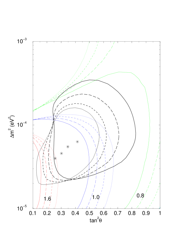
Figure 1: The best fit points and 3$\sigma$ allowed regions of oscillation parameters for different values of $\eta$: $\eta$ = 0.0 (solid line), 0.2 (long-dashed line), 0.4 (dashed line) and 0.6 (dotted line). Boron neutrino flux is taken as free parameters. Also shown lines of constant $f_{B}$ which minimize $\chi^{2}$.

Then we construct the $3\sigma$ regions in the $\Delta m^{2}-\tan^{2}\theta$ plane (Fig. 1) minimizing $\chi^{2}(\Delta m^{2},\tan^{2}\theta,f_{B})$ with respect to $f_{B}$: we denote the corresponding minimal value of $\chi^{2}$ by $\chi^{2}_{f}(\Delta m^{2},\tan^{2}\theta)$. Then $3\sigma$ contours are determined by $\chi^{2}_{f}(\Delta m^{2},\tan^{2}\theta)-\chi^{2}_{min}(\eta)=11.73$, where $\chi^{2}_{min}(\eta)$ is the minimum $\chi^{2}$ for a given value of $\eta$. We have found also lines of constant values of $f_{B}$ which minimize $\chi^{2}$ for a given $\eta$.

According to Fig. 1 and the Table 1, with increase of $\eta$ the allowed region shifts to smaller values of $\tan^{2}\theta$ and $\Delta m^{2}$. At the same time $f_{B}$ and $\chi^{2}_{min}$ increase.

$\eta$	0.0	0.2	0.4	0.6
$\chi^{2}$	65.1	65.5	67.5	72.6
$\Delta m^{2}\,(\times 10^{-5})$	6.3	5.5	4.6	4.0
$\tan^{2}\theta$	0.41	0.35	0.30	0.26
$f_{B}$	1.046	1.188	1.356	1.570

Table 1: Minimum $\chi^{2}$ for different values of $\eta$. Also presented are the values of parameters $\Delta m^{2}$, $\tan^{2}\theta$ and $\eta$ that minimize $\chi^{2}$.

These features can be well understood using Eqs. (15 - 16). Increase of $\eta$ [decrease of $(1-\eta)$] can be compensated by increase of $f_{B}$ and decrease of $P_{ee}$. Since $P_{ee}\sim\sin^{2}\theta$, the decrease of $P_{ee}$ implies decrease of mixing angle. With decrease of mixing the distortion of the spectrum (mainly the turn up of the probability at low energies) becomes stronger. This leads to shift of the allowed region to smaller values of $\Delta m^{2}$ (shift of the spectrum from the adiabatic edge).

Let us consider breaking of parameter degeneracy. Taking $P_{ee}\approx\sin^{2}\theta$ in expressions (16) and using results of the Table 1 we find values of parameters $x(\eta)$ and $y(\eta)$ for different $\eta$ in the best fit points (see Table 2). As follows from the Table 2 in the best fit points the parameters $x(\eta)$ and $y(\eta)$ are not invariant under changes of $\eta$: $x$ slightly increases (by $5\%$) whereas $y$ decreases significantly: almost by $50\%$. Another way to see these variations is to keep $x=\Phi_{CC}=constant$ and to exclude $P_{ee}$ from the combination $y$:

$$y=(1-\eta)(f_{B}-\Phi_{CC}).$$ (21)

Using $\Phi_{CC}=0.32$ we find $y(\eta)$ shown in the third line of the Table 2. Thus, the invariance of $x$ and $y$ (and therefore a degeneracy) is broken which leads the dependence of $\chi^{2}_{min}$ on $\eta$ and therefore to sensitivity of the analysis to the presence of sterile neutrinos.

$\eta$	0.0	0.2	0.4	0.6
$x$	0.304	0.308	0.313	0.320
$y$	0.742	0.703	0.623	0.492
$y(x=const)$	0.726	0.694	0.622	0.500

Table 2: Values of parameters $x$ and $y$ in the best fit points of global analysis for different values of $\eta$.

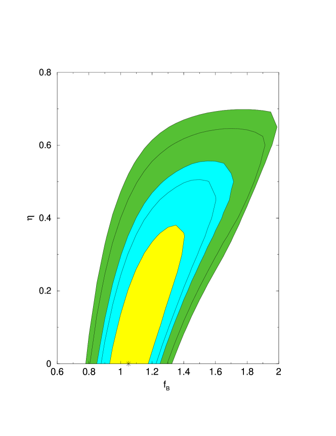
Figure 2: The allowed regions in $f_{B}-\eta$ plane, at 1$\sigma$, 90%, 95%, 99% and 3$\sigma$ C.L.. The best fit point (marked by star) is at $\eta=0$.

For fixed values of $\eta$ and $f_{B}$ we minimize $\chi^{2}$ with respect to $\Delta m^{2},\tan^{2}\theta$ which gives $\chi^{2}_{\Delta,\theta}=\chi^{2}_{\Delta,\theta}(\eta,f_{B})$. Using this function we construct contours of constant confidence level in $\eta,f_{B}$ plane (fig. 2). From this figure we get an upper limit for the sterile fraction

$$\eta<0.38\,(0.70),\,\,\,1\sigma\,\,(3\sigma)$$ (22)

The boron neutrino flux which correspond to maximal allowed value of $\eta$ equals $f_{B}=1.25$ ($1\sigma$) and $f_{B}=1.68$ ($3\sigma$).

We have performed minimization of $\chi^{2}$ with respect to $\Delta m^{2},\tan^{2}\theta$ and $f_{B}$, thus finding $\chi^{2}_{\Delta,\theta,f_{B}}=\chi^{2}(\eta)$. Then the function $\chi^{2}(\eta)$ allows to put the bounds for 1 d.o.f.:

$$\eta<0.26\,(0.64),\,\,\,1\sigma\,\,(3\sigma)$$ (23)

These results are very similar to results obtained in [16, 17]. In particular, it was found [16] that at $1\sigma$: $\eta_{max}=0.25$ for $f_{B}\sim 1.25$, and at $3\sigma$: $\eta_{max}=0.6$ for $f_{B}\sim 1.75$.

Imposing the SSM bound on the neutrino flux further strengthen the bound on “sterility”. It was found in [17]: $\eta<0.25$ at the $1\sigma$ and $\eta<0.5$ at the $3\sigma$ level. Notice that in fact $1\sigma$ bound is unchanged since at this level the required boron neutrino flux is within $1\sigma$ SSM prediction. In contrast, the limit becomes stronger at the $3\sigma$ level, where substantially larger than in SSM flux is needed.

For the SSM value of the boron neutrino flux, $f_{B}=1$, we get from the fig. 2 the following bounds on the sterile fraction: $\eta<0.14$ ($1\sigma$), $\eta<0.30$ ($2\sigma$), $\eta<0.47$ ($3\sigma$).

3.2 Who does not like sterile neutrino?

Let us identify observables which are sensitive to $\eta$. As we have discussed in sect. 2.1 these observables should contain information about the time variations or/and the energy dependence of the conversion effect. These dependences remove the degeneracy and therefore restrict $\eta$.

No statistically significant time variations have been found although some indications of the Day- Night asymmetry, $A_{ND}$, exist [26, 14]. Let us consider if $A_{ND}$ can restrict the admixture of sterile neutrino. The high energy neutrino data can be described by the $\nu_{e}$-survival probability during the day and during the night: $P_{ee}^{D}$, $P_{ee}^{N}$, or equivalently, by $\Delta P_{ee}\equiv P_{ee}^{N}-P_{ee}^{D}$ and $\bar{P}_{ee}\equiv(P_{ee}^{N}+P_{ee}^{D})/2$. Consequently, in Eq. (13 - 15) we should substitute $P_{ee}\rightarrow\bar{P}_{ee}$ and add to analysis an additional observable:

$$A_{ND}=\frac{\Delta P_{ee}}{\bar{P}_{ee}}.$$ (24)

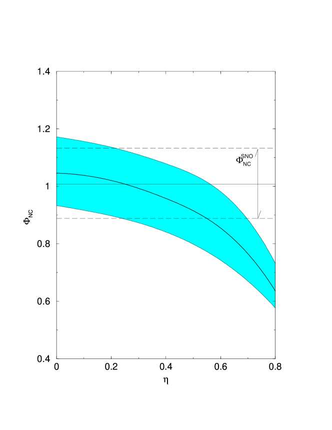
Figure 5: The predicted value of $\Phi_{NC}$ as a function of $\eta$. The band corresponds to the $1\sigma$ region. The horizontal lines show the present SNO result.

In the LMA region the average suppression is determined basically by mixing angle: $\bar{P}_{ee}\sim\sin^{2}\theta$, whereas the DN asymmetry depends mainly on $\Delta m^{2}$. This can be seen from lines of constant ratio $CC/NC\sim P_{ee}$ and lines of constant $A_{ND}$ which are nearly orthogonal each other (see figs. 5 and 6 from [21]). Therefore $\Delta P_{ee}$ and $\bar{P}_{ee}$ do not correlate and can be considered as independent fit parameters. For a given $\bar{P}_{ee}$, the difference $\Delta P_{ee}$ can change in the wide range, and the data on the asymmetry can be easily fitted. So, adding experimental information about the Day and Night asymmetry does not help to resolve degeneracy and therefore to improve the bound on $\eta$. Precise measurements of the zenith angle dependence of signal will change this conclusion.

No statistically significant distortion of the energy spectrum is found for $E>5$ MeV, which supports the degeneracy problem. The distortion (in experiments sensitive to $E>5$ MeV) is expected for higher values of $\Delta m^{2}$ and small mixing. However, substantial distortion is expected over wider detectable energy range which includes also the $pp-$ neutrinos. Therefore, the interplay of the high energy data and results from the low energy experiments should break the degeneracy.

To illustrate this effect, let us describe the distortion by two (for simplicity) different values of probabilities: at high energies, $P_{ee}^{H}$, and at low energies, $P_{ee}^{L}$ ($E<0.5$ MeV). The signal in the Gallium experiment is determined essentially by $P_{ee}^{L}$: so that the $Ge$-production rate equals $Q_{Ge}\propto P_{ee}^{L}$, and obviously, no substantial dependence on $f_{B}$ appears. In contrast to the Day-Night asymmetry case, the probabilities $P_{ee}^{L}$ and $P_{ee}^{H}$ are strongly (anti) correlated. Indeed, in the range of $pp$-neutrinos:

$$P_{ee}^{L}\sim 1-0.5\sin^{2}2\theta,$$ (25)

and since $P_{ee}^{H}\approx\sin^{2}\theta$ we get

$$P_{ee}^{L}\sim 1-2P_{ee}^{H}(1-P_{ee}^{H}).$$ (26)

With decrease of $P_{ee}^{H}$ the low energy probability $P_{ee}^{L}$ increases. Consequently, the predicted value of the $Ge$-production rate increases. Thus, combination of the Gallium and SNO data should break the degeneracy of parameters.

Now let us describe results of exact numerical calculations.

1). We have performed the $\chi^{2}$ analysis of the SNO data only. The best fit points in the oscillation plane as well as $f_{B}$ which minimize $\chi^{2}_{SNO}(\eta)$ are given for different values of $\eta$ in the Table 3. Notice that with increase of $\eta$ the quality of the fit does not change: $\chi^{2}$ even slightly decreases. So, as far as SNO data alone are concerned, no bound on $\eta$ appears. Variations of $\eta$ can be completely compensated by changes of $P_{ee}$ and $f_{B}$. The day-night asymmetry has low statistical significance.

$\eta$	0.0	0.2	0.4	0.6
$\chi^{2}$	25.6	25.4	25.3	25.1
$\Delta m^{2}\,(\times 10^{-5})$	4.5	4.5	4.0	3.6
$\tan^{2}\theta$	0.45	0.35	0.28	0.18
$f_{B}$	1.039	1.201	1.432	2.013

Table 3: Minimum $\chi^{2}_{SNO}$ for different values of $\eta$. Also presented are values of parameters $\Delta m^{2}$, $\tan^{2}\theta$ and $\eta$ that minimize the $\chi^{2}_{SNO}$.

The SNO experiment has higher sensitivity to the $NC$- events. For this reason the allowed region provided by SNO is restricted in $\tan^{2}\theta$ from both sides. Increase of $\eta$ has the effect of moving the allowed region to smaller values of $\tan^{2}\theta$, as can be seen in fig. 3.

Indeed, to keep the combinations (16) unchanged with increases of $\eta$ one needs (i) to diminish $P_{ee}$, which implies decrease of $\theta$ since in the LMA region $P_{ee}\sim\sin^{2}\theta$, (ii) to decrease $\Delta m^{2}$ to avoid distortion (turn up) of the spectrum at small energies and (iii) to increase $f_{B}$ to compensate decrease of $P_{ee}$.

2). In fig. 3 we show also lines of constant $Ge$-production rate. The rate increases with decrease of mixing. According to the figure, in the SNO allowed region for $\eta=0.6$ the rate $Q_{Ge}>75$ SNU and in the best fit point $Q_{Ge}=83$ SNU. For $\eta=0.4$ we get $Q_{Ge}=75$ SNU in the best fit point. The combined results from SAGE, Gallex and GNO experiments is $Q_{Ge}=(70\pm 4)$ SNU. So, the Gallium results prevent from further shift of the allowed region to smaller $\theta_{12}$ and therefore forbid larger $\eta$. To illustrate the role of Gallium experiments, we find the bounds on $\eta$ that can be derived by taking only SNO and Gallium data:

$$\eta<0.43\,(0.78),\,\,\,1\sigma\,\,(3\sigma),$$ (27)

which are weaker than those obtained by taking all the data (23).

In principle, further more precise measurements of the Ge-production rate could improve the bound on the sterile component.

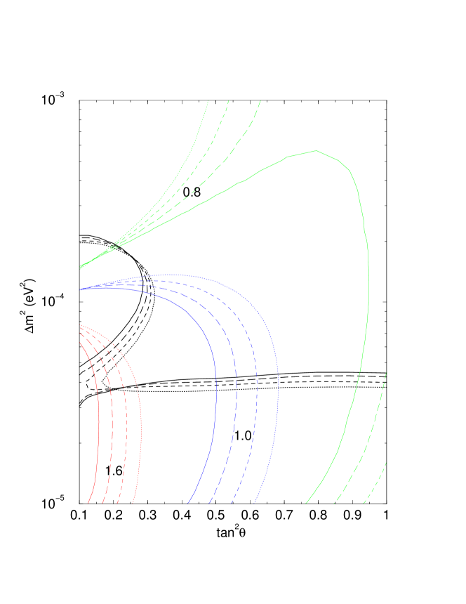
Figure 4: The 1$\sigma$ allowed region (right upper parts) from the analysis of the SuperKamiokande data for different values of $\eta$. Also shown are lines of constant $f_{B}$ which minimize $\chi^{2}$ fit of the SK data for different $\eta$.

3). Let us comment on the impact of SuperKamiokande. In fig. 4 we show result of analysis of the SuperKamiokande data only for different values of $\eta$. The excluded (at $1\sigma$) regions in the oscillation parameter space are due to the effects of spectrum distortion and the Earth $\nu_{e}$ regeneration. They are only slightly modified by the presence of sterile component. With increase of $\eta$ the excluded region shifts to larger mixing angles. This is related to the fact that with increase of sterile fraction the distortion of the spectrum increases due to decrease of the damping effect related to active neutrinos. The exclusion due to earth regeneration becomes weaker. Since for active-sterile system the effective matter potential is smaller the regeneration region shifts to smaller $\Delta m^{2}$. Correspondingly, lower bound of the allowed region shifts to smaller $\Delta m^{2}$.

In the allowed region, where distortion and time variations are small the data can be reproduced for different values of $\eta$ by adjusting $f_{B}$ and $P_{ee}$ (see (15)).

In fig. 4 we show also $f_{B}$ that gives the best fit to the Super-Kamiokande data. With increase of $\eta$ the lines $f_{B}=const$ shift to larger $\tan^{2}\theta$ and $\Delta m^{2}$ (where the survival probability is larger) to compensate decrease of muon and tau neutrino contribution. Large values of $\eta$ are allowed, when the boron neutrino flux is much larger than the SSM flux.

Similarly to the Gallium experiments, SuperKamiokande prevents from the shift of the allowed region to smaller mixings. Consequently, the combined fit of the SNO and SK will also give the bound on the sterile fraction. Comparison of the bounds (23) with and (27) without the SK result allows to evaluate the role of SuperKamiokande.

4). The Homestake experiment alone is not sensitive to $\eta$. However, it has some impact since its result restrict the oscillation parameters. The $Ar$-production rate decreases with mixing angle and the agreement with the Homestake result becomes even better with increase of $\eta$. Comparing the SNO and Homestake results we find that in the best fit SNO point for $\eta=0.6$ the rate equals $Q_{Ar}=2.75$ SNU which is within $1\sigma$ of the Homestake result. So, the SNO and Homestake data favor presence of sterile component.

Summarizing, the bound on sterility appears as combined effect of several experiments. In the global analysis the constrain on $\eta$ comes from the SNO measurements of the spectrum which contains information about the NC and CC event rate from the one hand side and Gallium as well as the SK experiment from the other side. With increase of $\eta$, SNO pushes the allowed region to smaller $\tan^{2}\theta$, whereas Gallium and SK experiments put lower bound on $\tan^{2}\theta$. For instance, the best SNO fit point for $\eta=0.6$ lies in the excluded Gallium region and at the border of the SK excluded region.

4 Future experiments and bounds on $\eta$

4.1 $NC$ measurements at SNO

SNO is taking data with much higher sensitivity to the $NC$ current events, and therefore precision of measurements of $\Phi_{NC}$ will be significantly improved. Clearly, distortion of the spectrum of the NC events will be signature of the sterile neutrino conversion. Although if LMA is the dominant solution, one does not expect observable effect. As far as total rate is concerned, the parameters can be adjusted in such a way that even more precise data can be reproduced for large $\eta$. Basically we will get the same shift of the allowed region as in fig. 1 but the size of the region around the the best fit point will be smaller. For this reason no drastic improvements of the bound on sterility is expected.

To evaluate the impact of future $NC$-measurements at SNO we show in fig. 5 the $1\sigma$ region of predictions of $\Phi_{NC}$ as a function of $\eta$ from the global fit. The results have been obtained in the following way. We use the global analysis of the solar neutrino data for different values of $\eta$, as is shown in fig. 1. Then we calculate $\Phi_{NC}$ in the best fit points (solid line) as well as the spread of predictions for $\Phi_{NC}$ within $1\sigma$ allowed region. Using the fig. 5, we find that the present $1\sigma$ experimental result on $\Phi_{NC}$, gives the upper bound $\eta<0.7$ which agrees with the $3\sigma$ bound from the global analysis. Assuming three times smaller error bars for the $NC$ measurements, $\Phi_{NC}=1\pm 0.03$, we get the bound $\eta<0.5$ which should be compared with present bound $\eta<0.64$.

4.2 KamLAND and sterile fraction

The signal at KamLAND is determined by the vacuum oscillation survival probability, so that the rate of events is

$$N=\sum_{i}\int dE\left(1-\sin^{2}2\theta_{12}\sin^{2}\frac{\Delta m^{2}_{12}L_{i}}{2E}\right)F_{i}\sigma A~{},$$ (28)

where $F_{i}$ is the flux from $i$ reactor, $\sigma$ is the cross-section of $\bar{\nu}p\rightarrow e^{+}n$ reaction, $A$ is the energy resolution function. The sum is taken over all reactors contributing to the flux at Kamioka and the integral denotes schematically the integrations over the neutrino energy, and the true energy of produced positron. This rate does not depend on $\eta$ or $f_{B}$. Being combined with the solar neutrino results it breaks degeneracy. KamLAND will fix the oscillation parameters $\Delta m^{2}_{12}$, $\tan^{2}\theta_{12}$, and consequently, will allow to predict $P_{ee}$ which describes the solar neutrino conversion.

Let us evaluate how combined analysis of the solar data and KamLAND can improve the bound on sterile component.

Let us introduce the suppression factor of total event rate above certain threshold:

$$R_{KL}(\Delta m^{2},\tan^{2}\theta)\equiv\frac{N(\Delta m^{2},\tan^{2}\theta)}{N_{0}}~{},$$ (29)

where $N$ is given in (28) and $N_{0}$ is the event rate in absence of oscillations.

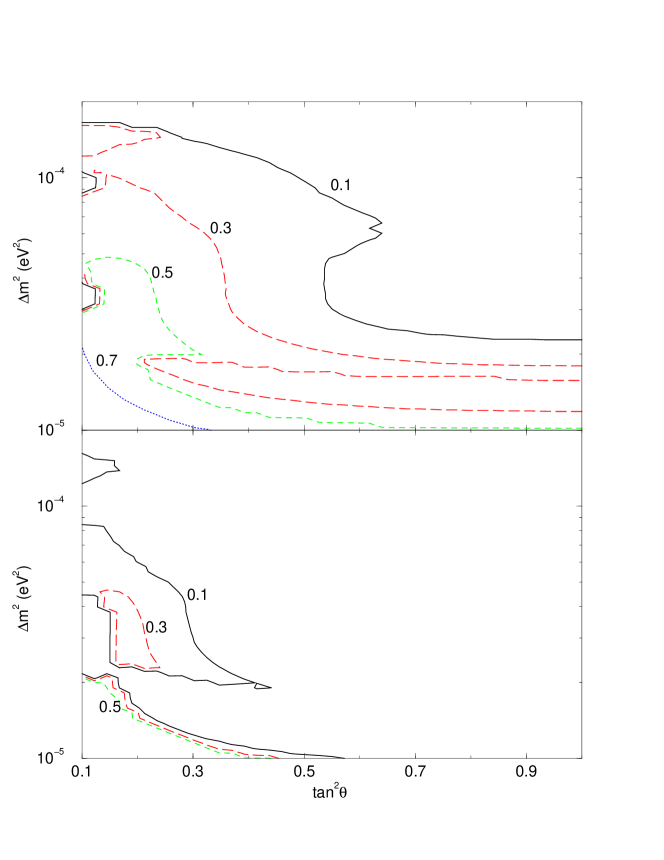
Figure 8: The upper panel: the lines of constant 1$\sigma$ upper bound (figures at the curves) on $\eta$ which can be obtained from from combined analysis of simulated KamLAND and solar neutrino results. The lower panel: the same as in the upper panel but for 1$\sigma$ lower bound on $\eta$.

Since predictions for KamLAND do not depend on the state to which the electron neutrino converts, we can use results of calculations of $R_{KL}$ for the pure active case [21]. In fig. 8 of paper [21] we have presented lines of constant $R_{KL}$ in $(\Delta m^{2},\tan^{2}\theta)$ plane. In the best fit points we find $R_{KL}(0)=0.66$, $R_{KL}(0.2)=0.63$, $R_{KL}(0.4)=0.55$, $R_{KL}(0.6)=0.52$. Due to decrease of $\Delta m^{2}$ in the best fit points, the expected value of the suppression in the KamLAND experiment becomes stronger.

To quantify impact of the event rate measurements at KamLAND we have constructed the $\chi^{2}(\Delta m^{2},\tan^{2}\theta,f_{B},\eta)$ as the function $R_{KL}$. Practically we impose the following condition $R_{KL}(\Delta m^{2},\tan^{2}\theta)=const$ which implies relation between $\Delta m^{2}$ and $\tan^{2}\theta$. So, for a given value $R_{KL}$ the $\chi^{2}$ is the function of $\Delta m^{2}$ or $\tan^{2}\theta$ only:

$$\chi^{2}=\chi^{2}(\tan^{2}\theta,R_{KL},f_{B},\eta).$$ (30)

For each value of $R_{KL}$ we minimize $\chi^{2}$ with respects to $\tan^{2}\theta,f_{B},\eta$ thus finding $\chi^{2}_{\theta,f_{B},\eta}(R_{KL})$. This function is shown in the upper panel of fig. 6. In the bottom panel the corresponding values of $f_{B}$ and $\eta$, which minimize $\chi^{2}$, are presented. For comparison in the upper panel we show also the function $\chi^{2}_{\theta,f_{B}}(R_{KL})$ for $\eta=0$.

The following remarks are in order.

For $R_{KL}<0.67$ the quality of the fit does not depend on $R_{KL}$. It corresponds to $\eta=0$ and $f_{B}\approx 1.05$. For $R_{KL}>0.67$, $\chi^{2}$ increases with $R_{KL}$. Simultaneously the best fit values of $\eta$ and $f_{B}$ increase. At $3\sigma$ level ($\chi^{2}=74$) we find maximal value of $R_{KL}$ and corresponding values of $\eta$ and $f_{B}$

$$R_{KL}\sim 0.75,~{}~{}~{}~{}\eta=0.35,~{}~{}~{}~{}f_{B}=1.4.$$ (31)

For $\eta=0$ the value $R_{KL}\sim 0.725$ is allowed. So, the introduction of sterile neutrino in the single $\Delta m^{2}$ approach does not lead to significant increase of maximal allowed value of $R_{KL}$. The goodness of the fit decreases sharply: e.g. for $R_{KL}=0.8$ we get $\Delta\chi^{2}=25$ even in presence of sterile component.

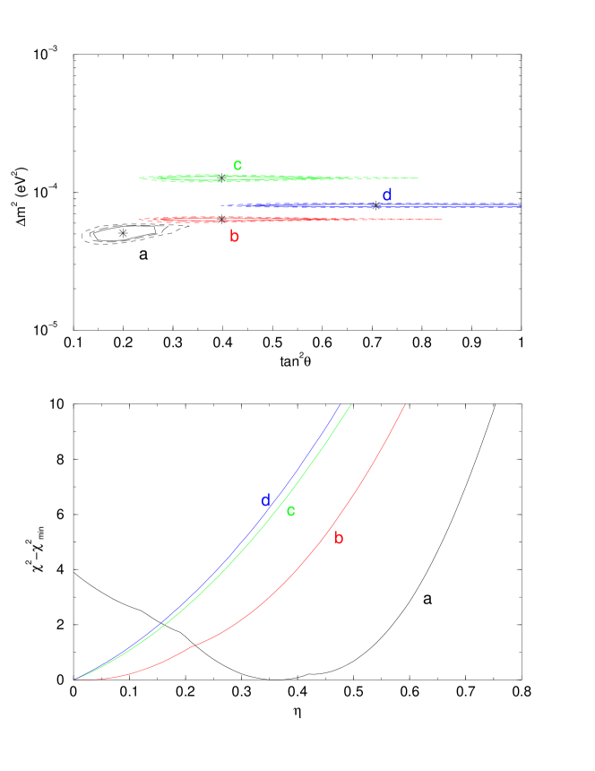
Figure 7: a) The $1\sigma,2\sigma,3\sigma$ allowed regions from the analysis of simulated KamLAND data. True values for the neutrino parameters that are indicated by a stars. b) The dependence of the $\chi^{2}$ on $\eta$ for these points from a combined analysis of the simulated KamLAND and the solar neutrino results.

Let us analyze how the KamLAND spectral measurements can help in constraining $\eta$. We have simulated the KamLAND spectral data for 4 different points a), b), c), d) in the $\Delta m^{2}-\tan^{2}\theta$ plane (marked by stars in fig. 7a)). In simulations we use statistics which can be collected during 3 years in 600 tons above the energy threshold for visible energy $E_{vis}=2.6$ MeV. In absence of oscillations this would correspond to 1170 events. We assumed a $4\%$ uncertainty in the overall normalization and a $2\%$ uncertainty in the energy scale. We have simulated the energy spectrum (for each point) using 12 bins of $0.5$ MeV size in the visible energy.

We perform $\chi^{2}$ analysis of simulated spectra assuming a full correlation of systematics uncertainties. We minimize

$$\chi^{2}_{KL}=\sum_{i=1,12}\sum_{j=1,12}R_{i}\sigma^{-2}_{i,j}R_{j}$$ (32)

and construct contours of constant $1\sigma$, $2\sigma$, $3\sigma$ confidence level around selected points in the $\Delta m^{2},\tan^{2}\theta$ plane (see fig. 7a). Notice that our allowed regions are somehow larger than those obtained in  [31, 32, 35], since we include systematic errors and also use higher threshold (smaller number of events). In agreement with results of calculations of other groups [31, 32, 35] we find that KamLAND will be able to measure $\Delta m^{2}$ rather precisely (if $\Delta m^{2}<2\cdot 10^{-4}$ eV²). At the same time determination of the mixing angle will not be very accurate. For the present best fit point $(b)$ we get from the figure $\tan^{2}\theta=0.28-0.60$ at the $1\sigma$ level, and $\tan^{2}\theta=0.25-0.85$ at the $3\sigma$ level.

Then we have performed combined analysis of the existing solar and simulated KamLAND data (notice that by the time KamLAND will have 3 years statistics new solar neutrino data will appear). For each selected point of the oscillation parameters in fig. 7a we calculate a global $\chi^{2}_{tot}$, which includes contributions from the solar neutrino analysis, $\chi^{2}_{Sun}$, and the KamLAND, $\chi^{2}_{KL},$:

$$\chi^{2}_{tot}=\chi^{2}_{KL}(\tan^{2}\theta,\Delta m^{2})+\chi^{2}_{Sun}(\tan^{2}\theta,\Delta m^{2},\eta,f_{B})\,\,.$$ (33)

For each value of $\eta$ we minimize $\chi^{2}_{tot}$ with respect to $\Delta m^{2}$, $\tan^{2}\theta$ and $f_{B}$. Results of this minimization as a function of $\eta$ are presented in fig. 7b. Let us comment on results for four selected points.

The point $b)$ is the best fit point of the global fit which corresponds to $\eta=0$. As follows from the figure,

$$\eta<0.19~{}(0.56)~{}~{}~{}1\sigma~{}(3\sigma),$$ (34)

thus improving the bound (23) from the solar data analysis only.

The points c) and d) are at larger $\Delta m^{2}$ and $\tan^{2}\theta_{12}$ as compared with b) thus further removed from the region preferred in the case of non-zero sterile component (small $\Delta m^{2}$ and $\tan^{2}\theta_{12}$). If KamLAND selects these points the bound on sterile component will be stronger than in a): $\eta<0.09~{}(0.45)$ at $1\sigma~{}(3\sigma)$.

The point a) is in the region preferable by sterile component. Selecting this point KamLAND will favor non-zero $\eta$. From the lower panel we get: $\eta=0.36^{+0.16}_{-0.12}$ at $1\sigma$ and $\eta>0$ at $2\sigma$ level. The $1\sigma$ lower bound is $\eta>0.24$.

For the points a) - d) we get the upper bounds on $\eta$: $\eta<0.08$ (c and d), $0.19$ (b) and $0.52$ (a). We have performed similar analysis for all the points of the oscillation parameter space. We show in fig. 8 the results as lines of constant upper bounds in the oscillation parameter plane. As a tendency, the bound becomes weaker with decrease of mixing and $\Delta m^{2}$. For sufficiently small $\tan^{2}\theta$ the best fit corresponds to a non-zero value of $\eta$ and the lower bound on $\eta$ appears. In the lower panel of fig. 8 we show such a lower limit for all points in $(\Delta m^{2},\tan^{2}\theta)$ plane.

5 Beyond single $\Delta m^{2}$ context

The results described in the previous sections can change if the electron neutrino mixes in the other mass eigenstates beyond the solar pair. Now more than one $\Delta m^{2}$ is involved, and effect depends on specific values of additional $\Delta m^{2}$.

In what follows we will assume that mixing of $\nu_{e}$ in the states $\nu_{3}$ and $\nu_{4}$ is small. Then if additional $\Delta m^{2}$ are outside the range of the MSW enhancement (e.g. $\Delta m^{2}_{14}$ is large) the effect of new $\nu_{e}$ mixing is small being suppressed by the mixing itself. If, however, $\Delta m^{2}_{14}$ is in the range of the MSW enhancement, the effect of additional mixing can be large. We will consider both possibilities.

5.1 Large additional $\Delta m^{2}$

Suppose $\nu_{e}$ has non-zero admixture in $\nu_{3}$ characterized by by $U_{e3}=s_{13}$. (Recall that $\nu_{3}$ is separated from the solar neutrino pair by the mass gap which corresponds to the atmospheric neutrino split.) We assume that $\nu_{e}$-admixture in $\nu_{4}$ is negligible so that the mass of $\nu_{4}$ can be arbitrary within the allowed range by non-solar neutrino experiment. We assume also that in the limit $s_{13}\rightarrow 0$, the state $\nu_{3}$ coincides with $\nu_{a}^{\prime}$ - the combination of $\nu_{\mu}$ and $\nu_{\tau}$, which is orthogonal to $\nu_{a}$ (7). In turn, $\nu_{4}$ is the combination of $\nu_{s}$ and $\nu_{a}$. As a result, we get the following mixing pattern:

$$\nu_{1} = \cos\theta_{12}(c_{13}\nu_{e}-s_{13}\nu_{a}^{\prime})-\sin\theta_{12}\nu_{x},$$

$$\nu_{2} = \sin\theta_{12}(c_{13}\nu_{e}-s_{13}\nu_{a}^{\prime})+\cos\theta_{12}\nu_{x},$$

$$\nu_{3} = c_{13}\nu_{a}^{\prime}+s_{13}\nu_{e},$$

$$\nu_{4} = \nu_{x}^{\prime},$$ (35)

where $\nu_{x}$ is defined in (6) and $\nu_{x}^{\prime}$ is the orthogonal to $\nu_{x}$ combination of $\nu_{s}$ and $\nu_{a}$. The mixing (35) differs from the generic case since $\nu_{e}$ and $\nu_{a}^{\prime}$ do not mix in $\nu_{4}$, and $\nu_{a}$ and $\nu_{s}$ do not mix in $\nu_{3}$.

The dynamics of propagation is similar to that of the case of three neutrinos. Indeed, let us represent $\nu_{e}$ in the following form:

$$\nu_{e}=c_{13}\nu_{e}^{\prime}+s_{13}\nu_{3}~{},$$ (36)

where $\nu_{e}^{\prime}=\cos\theta_{12}\nu_{1}+\sin\theta_{12}\nu_{2}~{}$ coincides with $\nu_{x}$, as can be easily checked. For the energies of solar neutrinos the matter effect on $s_{13}$ is negligible. Furthermore, the oscillations of solar neutrinos related to $\nu_{3}$ are averaged out. At the same time, $\nu_{e}^{\prime}$ and $\nu_{x}$ form standard two neutrino system with vacuum mixing and mater effects.

Using these features of dynamics, as well as projection of original flavor states onto $\nu_{e}^{\prime},\nu_{x},\nu_{3}$ one gets immediately the conversion probabilities:

$$P_{ee} = c_{13}^{4}\tilde{P}_{ee}+s_{13}^{4}$$

$$P_{es} = c_{13}^{2}\eta(1-\tilde{P}_{ee})$$

$$P_{ea} = c_{13}^{2}(1-\eta)(1-\tilde{P}_{ee})+s_{13}^{2}c_{13}^{2}(1+\tilde{P}_{ee}),$$ (37)

where $\tilde{P}_{ee}$ is the $\nu_{e}^{\prime}$-survival probability in the $\nu_{e}^{\prime}-\nu_{x}$ system: $\tilde{P}_{ee}=\tilde{P}_{ee}(\theta_{12},\Delta m^{2}_{12},\tilde{V})$ and $\tilde{V}=c_{13}^{2}V_{e}-V_{\mu}(1-\eta)$. As in the previous case, the parameter $\eta$ determines fraction of $\nu_{s}$ in the state $\nu_{x}$ to which $\nu_{e}^{\prime}$ converts, and also it gives total fraction of the $\nu_{s}$ in the solar pair (9).

Using (37), we get fluxes (in the units of the SSM flux) measurable by different reactions:

$$\Phi_{CC}=f_{B}[c_{13}^{4}\tilde{P}_{ee}+s_{13}^{4}],$$ (38)

$$\Phi_{NC}=f_{B}[1-(1-\tilde{P}_{ee})\eta c_{13}^{2}],$$ (39)

$$\Phi_{ES}=f_{B}[c_{13}^{4}\tilde{P}_{ee}+s_{13}^{4}+rc_{13}^{2}(1-\tilde{P}_{ee})(1-\eta)+rs_{13}^{2}(1+\tilde{P}_{ee})].$$ (40)

Comparing with Eq. (13,14, 15) we find that corrections are indeed of the order $s_{13}^{2}$. For the allowed values of $s_{13}^{2}$ these corrections have small impact on the data fit, as one can see from our analysis in [21].

The fluxes $\Phi_{CC}$, $\Phi_{NC}$, $\Phi_{ES}$ depend on two combinations of parameters, as in Eq. (17), with substitution $x\rightarrow x^{\prime}$, $y\rightarrow y^{\prime}$, where

$$x^{\prime}=c_{13}^{4}x,~{}~{}~{}~{}y^{\prime}=c_{13}^{2}+s_{13}^{2}(x+f_{B}),$$ (41)

and $x$ and $y$ are defined in (16). So, the problem of degeneracy is not resolved with $s_{13}$ corrections. Notice also that the fluxes in (38 - 40) satisfy the relation (18).

The KamLAND signal is determined by the survival probability

$$P_{ee}=c_{13}^{4}{P}_{2}+s_{13}^{4},$$ (42)

where $P_{2}$ is the two neutrino vacuum oscillation probability determined by $\Delta m^{2}_{12}$ and $\theta_{12}$. The factor $c_{13}^{4}$ leads to additional suppression of the KamLAND signal and shift of the allowed regions to smaller $\theta_{12}$ (see detailed analysis in the $3\nu$ context in [34]).

5.2 Small additional $\Delta m^{2}$

Let us consider the case when even small $\nu_{e}$ mixing beyond the solar pair can produce a strong effect. Suppose that,

(i) $\nu_{e}$ mixes with $\nu_{x}$ in the solar pair, $\nu_{1}$ and $\nu_{2}$, which has $\Delta m_{12}^{2}$ and $\tan^{2}\theta_{12}$ in the LMA region, as in (35);

(ii) the state $\nu_{4}\approx\nu_{x}^{\prime}$ (see (35)) is heavier than $\nu_{1}$ and the mass splitting is $\Delta m_{41}^{2}\sim 10^{-6}$ eV². (The mass $m_{1}$ can be very small or even zero). Furthermore, $\nu_{e}$ has small admixture in $\nu_{4}$: $\tan^{2}\theta_{14}\sim 10^{-3}$, so that $\nu_{e}-\nu_{x}^{\prime}$ oscillation parameters are in the SMA region.

(iii) the admixture of $\nu_{e}$ in the $\nu_{3}$ is zero (for simplicity).

Then, similarly to (35) we can write the mixing as

$$\nu_{1} = \cos\theta_{12}(c_{14}\nu_{e}-s_{14}\nu_{x}^{\prime})-\sin\theta_{12}\nu_{x},$$

$$\nu_{2} = \sin\theta_{12}(c_{14}\nu_{e}-s_{14}\nu_{x}^{\prime})+\cos\theta_{12}\nu_{x},$$

$$\nu_{3} = c_{13}\nu_{a}^{\prime},$$

$$\nu_{4} = c_{14}\nu_{x}^{\prime}+s_{14}\nu_{e}.$$ (43)

Here $\nu_{x}^{\prime}$ is the combination of $\nu_{a}$ and $\nu_{s}$ orthogonal to $\nu_{x}$ (6), and $\nu_{a}^{\prime}$ is the combination of $\nu_{\mu}$ and $\nu_{\tau}$ orthogonal to $\nu_{a}$ (7).

The system has two resonances associated with $\Delta m_{12}^{2}$ and $\Delta m_{41}^{2}$. Let us estimate qualitatively the conversion effect in different energy ranges.

In the first resonance related to $\Delta m_{12}^{2}$ the conversion is completely adiabatic. So, at the high energies, $E>7-8$ MeV, where crossing of the resonance occurs the survival probability equals $P_{ee}^{H}\approx\sin^{2}\theta_{12}$. At low energies, $E<0.5$ MeV, (no 12-resonance crossing) effect driven by $\Delta m_{12}^{2}$ is reduced to averaged vacuum oscillations. The result of conversion is similar to the one in usual three neutrino system:

$$P_{ee}^{L}=c_{12}^{4}P_{2}^{\prime}+s_{12}^{4},$$ (44)

where $P_{2}^{\prime}$ is the survival probability in the resonance related to $\Delta m_{14}^{2}$. It has a typical form of the survival probability of the SMA solution and characterized by $\Delta m_{14}^{2}$ and mixing parameter $\tan^{2}\theta=\tan^{2}\theta_{14}/\cos^{2}\theta_{12}$. Appearance of $P_{2}^{\prime}$ in this expression leads to an additional suppression of the $pp$-neutrino flux.

In the intermediate energy range, $E=(0.5-7)$ MeV, the conversion driven by $\Delta m_{14}^{2}$ will lead to flattening of the adiabatic edge of the suppression pit due to $\Delta m_{12}^{2}$.

5.3 KamLAND result and LMA

In the best fit point of the LMA region we predict $R_{KL}=0.66$ for zero $\eta$ [21]. At $3\sigma$ level $R_{KL}<0.73$. In presence of the sterile component this bound can be slightly relaxed: $R_{KL}<0.76$. For other solutions of the solar neutrino problem we predict $R_{KL}\approx 1.0$ if $s_{13}=0$. For non-zero $s_{13}$ the oscillations driven by $\Delta m^{2}_{atm}$ will lead the averaged oscillation result at KamLAND: $R_{KL}=1-0.5\sin^{2}2\theta_{13}$. For maximal allowed values of $s_{13}$ we get $R_{KL}=0.90-0.95$ depending on $\Delta m^{2}_{atm}$. What if $R_{KL}=0.76-0.90$ will be found?

The following comments are in order:

If solution of the solar neutrino problem is in the LMA region, a strong suppression is expected in KamLAND. In this case, introduction of additional sterile states will not help in the single $\Delta m^{2}$ context, as we have found in the Sect. 3.

Let us discuss what happens if two or more $\Delta m^{2}$ contributes.

Oscillation parameters can be taken beyond the LMA region in such a way that suppression in the KamLAND experiment is weaker. In this case, however, the conversion of solar neutrinos will not describe data in the two neutrino context. Then the parameters (mass, flavor mixing) of the $\nu_{4}$ can be selected in such a way that conversion driven by $\nu_{4}$ will not change KamLAND result but correct description of the solar data.

Such a possibility can be realized in the scheme described in the previous section 5.2 with $\Delta m_{12}^{2}\sim 6\cdot 10^{-5}$ eV². Indeed the KamLAND result is determined by the oscillations driven by $\Delta m_{12}^{2}$ and $\theta_{12}$. For $\tan^{2}\theta_{12}\sim 0.10-0.15$ we get $R_{KL}=0.80-0.85$.

As far as the solar neutrino signal is concerned, the high energy signal will be suppressed by $\sin^{2}\theta$, so that large boron neutrino flux: $f_{B}\sim 1.6$ is required to explain the SNO and SK results. According to our previous consideration, in the single $\Delta m^{2}$ context this point would be excluded by the Gallium experiment (large $Q_{Ge}$) and by SK (distortion of spectrum). The effect of $\Delta m_{14}^{2}$ changes a situation: appearance of $P_{2}^{\prime}$ in expression for probability at low energies (44) leads to an additional suppression of the $pp$-neutrino flux, and consequently, $Q_{Ge}$ rate. In the intermediate energy range, $E=(0.5-7)$ MeV, the conversion driven by $\Delta m_{14}^{2}$ will relax the SuperKamiokande lower bound on mixing which follows from absence of spectrum distortion. The detailed analysis of this possibility will be given elsewhere [36].

Another possibility to reconcile an intermediate suppression of signal in KamLAND and explanation of the solar neutrino data is to split two problems. Suppose the solar pair has $\Delta m_{12}^{2}$ in the LOW or VO regions, so that it does not produce any effect in KamLAND. The state $\nu_{4}$ which consists predominantly of the sterile component has the mass split: $\Delta m_{14}^{2}>10^{-4}$ eV². Then the suppression of the KamLAND signal is determined by admixture of $\nu_{e}$ in $\nu_{4}$: $R_{KL}=0.5\sin^{2}2\theta_{14}$. For instance, $R_{KL}=0.85$ can be achieved at $\sin^{2}\theta_{14}=0.09$. Effect in solar neutrinos will be determined by $P_{ee}^{sun}=c_{14}^{4}P_{ee}+s_{14}^{4}$, where $P_{ee}$ is the survival probability for the conversion driven by $\Delta m_{12}^{2}$. Additional factor $c_{14}^{4}\sim 0.8$ can even improve the fit of the data for LOW and SMA [21].

6 Conclusions

1. We have studied properties of mixing of the sterile and active neutrinos. In the single $\Delta m^{2}$ context (when electron neutrino is present in two mass eigenstates only) the problem is reduced precisely to two neutrino problem with mixing of $\nu_{e}$ with $\nu_{x}$ in the solar pair ($\nu_{x}$ is the combination of the active and sterile neutrinos).

2. We have performed the global fit of the solar neutrino data in the single $\Delta m^{2}$ context, treating the boron neutrino flux as a free parameter. The best fit corresponds to zero admixture of sterile component, $\eta=0$. We get the upper bound $\eta<0.26~{}(0.64)$ at $1\sigma~{}~{}(3\sigma)$. With increase of $\eta$ the best fit point shifts to smaller $\Delta m^{2}$ and $\tan^{2}\theta_{12}$.

3. Due to degeneracy of parameters, no one single observable gives the bound on $\eta$. The bound on sterility appears as an interplay of the SNO results whose allowed region of the oscillation parameters shifts to smaller mixings and $\Delta m^{2}$ with increase of $\eta$ and Gallium as well as SK results which restrict the mixing and $\Delta m^{2}$ from below.

4. Further more precise measurements of the $NC$ event rate at SNO will strengthen the bound: $\eta<0.5$ ($3\sigma$).

5. Implications of KamLAND depend on specific results of KamLAND measurements. If KamLAND result (rate, spectrum) corresponds to the best fit point of the solar neutrino analysis, then after 3 years of the KamLAND operation the limit will be strengthened down to $\eta<0.19~{}~{}(0.55)$ at $1\sigma~{}~{}(3\sigma)$. The limit will be stronger if the KamLAND best fit point will be at larger $\tan^{2}\theta_{12}$ and $\Delta m^{2}$ than the solar neutrino data give at present. In contrast, if KamLAND selects smaller $\tan^{2}\theta_{12}$ and $\Delta m^{2}$, the limit will be weaker, and moreover, the data may prefer non-zero sterile admixture.

6. The presence of sterile neutrinos (in the single $\Delta m^{2}$ context) relaxes the upper bound on the predicted rate $R_{KL}$ only weakly from 0.73 to 0.76 $(3\sigma)$. Larger values of $R_{KL}$ can be reached in the two $\Delta m^{2}$ context.

7. If electron neutrino mixes also in other mass eigenstates, the effects depend substantially on values of other $\Delta m^{2}$.

If additional $\Delta m^{2}_{14}\gg\Delta m^{2}_{12}$ the small corrections appear to formulas with a single $\Delta m^{2}$ which are proportional to the mixing of $\nu_{e}$ in additional mass eigenstates, e.g., $s_{13}^{2}$. If $\Delta m^{2}$, is in the MSW range an additional mixing can be resonantly enhanced in matter producing much larger effect. In this case intermediate values of $R_{KL}$ can be obtained.

Figure 3: The 1$\sigma$ allowed region from the analysis of the SNO data only for $\eta=0$ (straight line), 0.2 (long dashed), 0.4 (dashed) and 0.6 (dotted). Also shown are lines of constant $Q_{Ge}$.

Figure 6: a) Minimum $\chi^{2}$ obtained from analysis of the solar neutrino data as a function of the KamLAND rate, $R_{KL}$, $\eta=0$ (dashed line) and for $\eta$ taken as a free parameter (solid line). b) Value of $\eta$ (solid line and left axis) and $f_{B}$ (dashed line and right axis) that minimize the $\chi^{2}$ presented in the panel a).

References

- [1] LSND Collaboration, Phys.Rev. D64 (2001) 112007.
- [2] For recent discussion see M. Maltoni, T. Schwetz, M. A. Tortola,, J. W. F. Valle, Nucl. Phys. B 643, 321-338; M. C. Gonzalez-Garcia, M. Maltoni, C. Peña-Garay, Phys. Rev.D64, 093001 (2001), hep-ph/0105269.
- [3] W. Grimus and L. Lavoura, Phys. Rev D. 62 (2000) 093012; J. High Energy Phys. 09 (2000) 007, J. High Energy Phys. 07 (2001) 045; S. F. King, Nucl. Phys. B 576 (2000) 85; S. F. King and N. Singh, Nucl.Phys. B591 (2000) 3; H. S. Goh, R. N. Mohapatra, S.-P. Ng, Phys. Lett. B542 (2002) 116.
- [4] E. Ma, Phys. Lett. B 380 (1996) 286; Z. Chacko and R. Mohapatra, Phys. Rev. D 61 (2000) 053002.
- [5] R. Foot and R.R. Volkas, Phys. Rev. D52, 6595 (1995); Z.G. Berezhiani and R.N. Mohapatra, Phys. Rev. D52, 6607 (1995); V. Berezinsky and A. Vilenkin, Phys. Rev. D62, 083512 (2000); V. Berezinsky, M. Narayan and F. Vissani, hep-ph/0210204.
- [6] E. J. Chun, A. S. Joshipura, A. Yu. Smirnov, Phys. Rev. D54:4654 (1996).
- [7] K. Benakli, A. Yu. Smirnov, Phys. Rev. Lett. 79:4314 (1997), A. Lukas, P. Ramond, A. Romanino, G. G. Ross, Phys.Lett. B495 (2000) 136.
- [8] K. R. Dienes, E. Dudas and T. Gherghetta, Nucl. Phys. B557, 25 (1999); N. Arkani-Hamed, S. Dimopoulos, G. Dvali and J. March-Russel, Phys. Rev D 65 (2002) 024032, G. Dvali and A. Yu. Smirnov, Nucl.Phys. B563 (1999) 63.
- [9] K.R.S. Balaji, A. Perez-Lorenzana, A.Yu. Smirnov, Phys. Lett. B509:111, 2001.
- [10] S. M. Bilenky, C. Giunti, Phys. Lett. B320:323-328, 1994.
- [11] S. M. Bilenky, C. Giunti, Z.Phys. C68:495, 1995.
- [12] S. M. Bilenky, C. Giunti, Talk given at 4th International Workshop on Theoretical and Phenomenological Aspects of Underground Physics (TAUP 95), Toledo, Spain, 17-21 Sep 1995. Nucl.Phys.Proc.Suppl.48:381,1996, e-Print Archive: hep-ph/9512349.
- [13] Q. R. Ahmad et al., SNO collaboration, Phys.Rev.Lett. 89: 011301 (2002).
- [14] Q. R. Ahmad et al., SNO collaboration, Phys.Rev.Lett. 89: 011302 (2002).
- [15] V. Barger, D. Marfatia and K. Whisnant, Phys.Rev.Lett. 88 (2002) 011302
- [16] J. N. Bahcall, M. C. Gonzalez-Garcia, C. Peña-Garay, Phys.Rev. C66 (2002) 035802.
- [17] M. Maltoni, T. Schwetz, M.A. Tortola, J.W.F. Valle, hep-ph/0207227.
- [18] The idea to improve an upper bound on sterile fraction using KamLAND and solar neutrino results has been proposed by A. McDonald, July 2001, private communications.
- [19] CHOOZ Collaboration, M. Apollonio et al., Phys.Lett. B420, 397 (1998).
- [20] BUGEY Collaboration, B. Achkar et. al, Nucl. Phys. B434 (1995) 503.
- [21] P. C. de Holanda, A. Yu. Smirnov, hep-ph/0205241, to be published in Phys.Rev D.
- [22] B. T. Cleveland et al Astroph. J. 496 (1998) 505; K. Lande et al, in Neutrino 2000 [23], p.50.
- [23] A. B. McDonald, Proc. of the 19th Int. Conf. on Neutrino Physics and Astrophysics, Neutrino 2000 , Sudbury, Canada 2000, Nucl. Phys. B (Proc. Suppl.) 91 (2001) 21.
- [24] J.N. Abdurashitov et al. (SAGE collaboration), astro-ph/0204245.
- [25] C. M. Cattadori et al., in Proceedings of the TAUP 2001 Workshop, (September 2001), Gran-Sasso, Assesrgi, Italy.
- [26] S. Fukuda et al. (Super-Kamiokande collaboration) Phys. Rev. Lett. 86: 5651, 2001; Phys. Rev. Lett. 86: 5656, 2001.
- [27] Q. R. Ahmad et al., SNO collaboration, Phys. Rev. Lett. 87:071301, 2001.
- [28] J. N. Bahcall, M.H. Pinsonneault and S. Basu, Astrophys. J. 555 (2001)990.
- [29] L. E. Marcucci et al., Phys. Rev. C63 (2001) 015801; T.-S. Park, et al., hep-ph/0107012 and references therein.
- [30] KamLAND, P. Alivisatos, et. al., STANFORD-HEP-98-03, RCNS-98-15, 1998, S.A. Dazeley for the collaboration, hep-ex/0205041.
- [31] V. D. Barger, D. Marfatia, B. P. Wood, Phys. Lett. B498:53, (2001).
- [32] A. de Gouvea, C. Pena-Garay, Phys. Rev. D64:113011, (2001).
- [33] H. Murayama, A. Pierce, Phys.Rev.D65:013012,2002
- [34] M.C. Gonzalez-Garcia, C. Pena-Garay, Phys. Lett.B527:199, (2002).
- [35] P. Aliani, et. al., hep-ph/0211062.
- [36] P. C. de Holanda and A. Yu. Smirnov, in preparation.