CERN-TH/2002-332
MCTP-02-60
Observational Tests of Open Strings in Braneworld Scenarios

Abstract

We consider some consequences of describing the gauge and matter degrees of freedom in our universe by open strings, as suggested by the braneworld scenario. We focus on the geometric effects described by the open string metric and investigate their observational implications. The causal structure of spacetime on the brane is altered; it is described not by the usual metric $g_{\mu\nu}$, but instead by the open string metric, that incorporates the electromagnetic background, $G_{\mu\nu}=g_{\mu\nu}-(2\pi\alpha^{\prime})^{2}(F^{2})_{\mu\nu}$. The speed of light is now slower when propagating along directions transverse to electromagnetic fields or an NS-NS two form, so that Lorentz invariance is explicitly broken. A generalized equivalence principle guarantees that the propagation of all particles, not just photons, (with the exception of gravitons) is slower in these transverse directions. We describe experiments designed to detect the predicted variations in the causal structure: interferometric laboratory based experiments, experiments exploiting astrophysical electromagnetic fields, and experiments that rely on modification to special relativity. We show that current technology cannot probe beyond open string lengths of $10^{-13}$ cm, corresponding to MeV string scales. Should the experiments someday be able to observe these effects, one could use them to determine the string scale. We also point out that in a braneworld scenario, constraints on large scale electromagnetic fields together with a modest phenomenological bound on the NS-NS two-form naturally lead to a bound on the scale of canonical noncommutativity that is two orders of magnitude below the string length. By invoking theoretical constraints on the NS-NS two-form this bound can be improved to give an extremely strong bound on the noncommutative scale well below the Planck length, $\sqrt{|\theta|_{max}}<10^{-35}\,{\rm cm}\times\left({{\rm TeV}\over{\rm string}\,\,{\rm scale}}\right)^{2}$.

1 Introduction

Although string theory is a very promising theoretical framework for describing quantum gravity and the unification of particles and their interactions, it has so far been unsuccessful in making contact with our observable universe. The purpose of this paper is to look for observational signatures of string physics. In particular we have in mind the perspective of the recently proposed braneworld scenario [1]. In this scenario, our observable universe is a three-dimensional surface (3-brane) embedded in a higher dimensional curved spacetime. The brane degrees of freedom are described by open strings that end on the brane. Here the gauge and matter degrees of freedom of the standard model, all described by open strings [2], live on the brane. Gravitons, which are closed string modes, propagate in the bulk. The smallness of gravitational interactions in our brane universe can be explained either by the size of compact extra dimensions or by the warping of the space transverse to the brane (effectively reducing the strength of gravitational interactions to the Planck scale on our observable brane [3]). In the latter setup, it is possible to start out with a fundamental scale in higher dimensions, in our case the string scale, equal to a few TeV. In this paper we consider string scales in the range TeV to $m_{\rm{pl}}=10^{19}$ GeV.

The fact that all matter and radiation in a braneworld universe are described by open string states leads to some interesting consequences. As pointed out long ago, the effective action for the massless modes of open strings in a slowly varying $U(1)$ background is given by the Born-Infeld (BI) action.

Causal Structure of Spacetime: The most important effect of open string states for the purposes of this paper is that the causal structure of our brane is altered; it is described not by the usual metric, $g_{\mu\nu}$, but instead by the open string metric, $G_{\mu\nu}$ [8] that incorporates the electromagnetic background, $F$. Hence the (3+1)-dimensional metric describing propagation in our universe (3-brane) is given by

$$G_{\mu\nu}=g_{\mu\nu}-(2\pi\alpha^{\prime})^{2}(F^{2})_{\mu\nu}\,,$$ (1)

where Greek indices $\mu=0,1,2,3$ describe our (3+1)-dimensional spacetime. The anti-symmetric tensor $F_{\mu\nu}={\cal F}_{\mu\nu}-{\cal B}_{\mu\nu}^{NS}$ is constructed out of the electromagnetic field tensor on the brane ${\cal F}=dA$ and the NS-NS anti-symmetric 2-form gauge potential ${\cal B}_{\mu\nu}^{NS}$ induced from the bulk. The parameter $\alpha^{\prime}$ represents the squared string length which we take to be in the range

$$10^{-33}\,{\rm cm}<l_{s}\equiv\sqrt{\alpha^{\prime}}<10^{-17}\,{\rm cm}\,.$$ (2)

Here the lower limit corresponds to a string scale at $m_{\rm pl}$ while the upper limit corresponds to a TeV string scale.

As we will show, the speed of light is now slower when propagating along directions transverse to electromagnetic fields. Assuming that the ${\cal B}_{\mu\nu}^{NS}$ contribution vanishes, we find the following expression for the speed of light along directions at an angle $\theta$ from the magnetic and/or electric field vectors ($\vec{E}||\vec{B}$)

$${\bar{c}\over c_{\rm vac}}=\sqrt{{1-(2\pi\alpha^{\prime})^{2}E^{2}\over 1+(2\pi\alpha^{\prime})^{2}(B^{2}\sin^{2}{\theta}-E^{2}\cos^{2}{\theta})}}\,\,.$$ (3)

For the specific case of $\theta=\pi/2$, the modified speed of light is

$$\bar{c}=c_{\rm{vac}}\sqrt{\frac{1-(2\pi\alpha^{\prime})^{2}E^{2}}{1+(2\pi\alpha^{\prime})^{2}B^{2}}}\approx[1-2(\alpha^{\prime}\pi)^{2}(E^{2}+B^{2})]c_{\rm{vac}}$$ (4)

where the $E$ and $B$ fields are at right angles to the propagating light, and the approximation is made in the limit of small $\alpha^{\prime}\,E$ and $\alpha^{\prime}\,B$.

Note that the component of light propagation parallel to the electromagnetic field is unaffected; hence, we are explicitly breaking Lorentz invariance in an interesting way. As light emerges from a point source in the presence of strong electromagnetic fields, the surface defined by the distance it has traveled in a given time (the horizon) is no longer a spherical shell, but rather has the shape of an ellipsoid (even after the light leaves the vicinity of the fields, it retains this ellipsoidal shape).

We emphasize that the propagation of all particles (with the exception of gravitons) is slower in directions perpendicular to electromagnetic fields [16]: It is the causal structure of spacetime on the brane that is modified, and hence the behavior of all matter and radiation is altered. This effect is a property of spacetime and not of photons. One way to visualize this effect is shown in Figure 1: the lightcone is “pinched” in certain directions; i.e., the conventional 45 degree angle between the spatial and temporal axes becomes smaller. This pinching takes place in all directions other than parallel to the electromagnetic field.

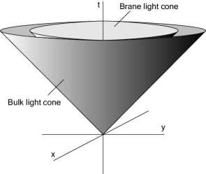
Figure 1: The pinching of light cones in the presence of electromagnetic fields. The pinching occurs in all directions not parallel to the field. Here the fields are confined to the (x-y) plane and point out of the page.

We describe several experiments designed to search for this effect. In general, this effect is suppressed because it is proportional to the string length to the fourth power, as can be seen in Eq.(4). We will show that current experiments are able to achieve sensitivity to a string length of $10^{-13}$ cm, corresponding to a string scale of 100 MeV. Hence, many orders of magnitude of improvement in technology or entirely new methods would be required to observe anything interesting. We will discuss (i) interferometric laboratory based experiments, (ii) experiments exploiting astrophysical electromagnetic fields, and (iii) experiments that rely on modification to special relativity. Because strong EM fields modify the causal structure of spacetime, classical tests of relativity are altered; in particular, we examine the fractional change in the muon lifetime when immersed in a strong magnetic field.

We also note that, although nonlinear quantum electrodynamics (QED) produces similar but much larger effects, they are in principal distinguishable from the geometric effects described here. First, nonlinear QED applies only to photons, whereas the effects described in this paper are a result of changes in spacetime itself: these spacetime effects apply equally to all particles (other than gravitons) and produce corrections, e.g. to special relativity, that cannot possibly be produced by QED. In addition, because these spacetime effects do not give rise to birefringence, whereas the nonlinear QED effects do, they could in principle be differentiated even in the case of photons.

Gravitons: The only particles not slowed in the presence of electromagnetic fields are gravitons. Gravitons live in the bulk rather than on the brane and do not feel the previously described changes in causal structure. Hence their propagation time, e.g., from a supernova explosion with strong electromagnetic fields, will be faster than the propagation time of all other particles. As discussed below, one can hope to detect the time delay between the arrival times of neutrinos and gravitons from supernovae. Such delay effects were also considered by Chung and Kolb [9] in the context of Lorentz violations in braneworlds and by Csaki, Erlich, and Grojean [30] in the similar context of asymmetrically warped spacetimes. Following a somewhat different approach, Burgess et al. [31] have explored constraints on the graviton dispersion relations arising from Lorentz violations in the bulk and how such violations are ultimately transmitted to fermion and photon dispersion relations.

Chung and Freese [10] studied a different effect causing the effective speed of light to be modified. They proposed “shortcut metrics”, whereby geodesics traversing the extra dimensions can allow communication between points on the brane that are naively causally disconnected. They [10] proposed these metrics as an alternative to inflationary scenarios as a solution to the horizon problem. Subsequent work on shortcut metrics includes [11], [12], [13], and [14]. Shortcut metrics and electromagnetic fields share the feature of having propagation of signals via the bulk faster than signals remaining on the brane. However, shortcut metrics have the end effect of allowing light signals to appear to travel faster than usual (by traversing the bulk) while electromagnetic fields have the effect of slowing down light signals.

Noncommutative Geometry:

As emphasized by Seiberg and Witten [8] in the context of open string theory, an electromagnetic background can be related to the noncommutativity of spacetime,

$$[x^{\mu},x^{\nu}]=i\theta^{\mu\nu}\,$$ (5)

via

$$\theta^{\mu\nu}=2\pi\alpha^{\prime}\left(-2\pi\alpha^{\prime}F^{\mu\rho}(G^{-1})^{\mu}_{\rho}\right)\,,$$ (6)

where $\theta^{\mu\nu}$ is the noncommutativity parameter and $G^{\mu\nu}$ is given in Eq.(1). Astrophysical electromagnetic fields together theoretical constraints on the NS-NS 2-form ${\cal B}_{\mu\nu}^{NS}$ can then be used to place extremely strong bounds on the parameter $\theta^{\mu\nu}$. The absence of cosmological electric fields of any significant amplitude makes any numerical bound on the timelike component $\theta^{0i}$ so extremely tiny that we conclude it is essentially vanishing. From astrophysical magnetic fields $B$, we can present an explicit numerical bound on the scale of spacelike noncommutativity $\theta^{ij}$. For magnetic backgrounds, we find

$$|\theta|=\sqrt{2}\,(2\pi\alpha^{\prime})^{2}\,|B|\,.$$ (7)

The typical size of intergalactic magnetic fields is roughly $|B|_{IG}\leq 10^{-9}$ Gauss, so that we find the following upper bound on the length scale of spacelike noncommutativity

$$\sqrt{|\theta|_{max}}\leq 10^{-35}\,\left[{{\rm stringscale}\over{\rm TeV}}\right]^{-4}\,{\rm cm}\,.$$ (8)

This is an amazingly strong bound on the scale of noncommutativity. Even without invoking the theoretical constraint on the 2-form ${\cal B}_{\mu\nu}^{NS}$, but instead using a more modest phenomenological bound on the scale of ${\cal B}_{\mu\nu}^{NS}$ based on the absence of strong (anisotropic) effects on the causal structure of spacetime, we still find that the scale of noncommutativity has to be below the string length.

Outline: The organization of this paper is as follows; we begin by considering open strings ending on D-branes, concentrating on the $U(1)$ part of the dynamics giving the Born-Infeld action for the massless modes of the strings. We next introduce the open string metric, briefly explain its relevance for finding decoupled noncommutative field or string theories, and show exactly how the open string metric affects the causal structure on the brane. In the following section we describe experiments designed to detect the nonlinear effects predicted by the open string metric. Finally, we describe a strong bound on the magnitude of the noncommutativity parameter by using experimental data on large scale electromagnetic fields. We end with some conclusions.

2 D-branes and the open string metric

Our working assumption will be that our $4$-dimensional universe is a (wrapped) D-brane embedded in a higher dimensional curved spacetime, as suggested by the braneworld scenario. All degrees of freedom confined to the D-brane, and therefore our universe, are described by open string states. For the present discussion we can limit ourselves to the subset of bosonic gauge degrees of freedom (i.e. photons), because everything we will conclude about the causal structure can be generalized to include all open string degrees of freedom. We refer to [15] for a more complete discussion of strings in electromagnetic backgrounds. When the background fields vary slowly enough with respect to the string length $l_{s}$, the massless bosonic modes of the string (photons) can be shown to obey equations of motion that can be deduced from the following effective Born-Infeld Lagrangian [4]

$${\cal L}_{BI}=T\,\sqrt{-{\rm det}\,(g_{\mu\nu}+(2\pi\alpha^{\prime})F_{\mu\nu}})\,,$$ (9)

where $T$ is the brane tension and $g_{\mu\nu}$ is the induced metric on the brane, defined by the bulk metric $\gamma_{KL}$ and the embedding scalars $X^{K}$ as $g_{\mu\nu}=\partial_{\mu}X^{K}\partial_{\nu}X^{L}\gamma_{KL}$. Here, Greek indices $\mu=0,1,2,3$ and Latin indices $K=0,1,2,3,...$ extend also over the extra dimensions. The anti-symmetric tensor $F_{\mu\nu}={\cal F}_{\mu\nu}-{\cal B}_{\mu\nu}^{NS}$ is constructed out of the electromagnetic field tensor on the brane ${\cal F}=dA$ and the NS-NS anti-symmetric 2-form gauge potential ${\cal B}_{\mu\nu}^{NS}$ induced from the bulk. This particular combination is the only one invariant under the string worldsheet gauge transformations in the presence of D-branes.

It will be important in later sections to distinguish between the pure electromagnetic contribution that can be probed or detected with charged open string states (e.g. electrons), and the NS-NS 2-form contribution to the BI action. Charged open string states correspond to strings stretching between two different branes $i$ and $j$ and couple electromagnetically to ${\cal F}^{i}-{\cal F}^{j}$. In the simplest case of two branes with two $U(1)$’s on the two seperate brane worldvolumes, the relative difference ${\cal F}^{i}-{\cal F}^{j}$ corresponds to the $U(1)$ electrodynamics that we are interested in, whereas the symmetry under shifts of the overall position of the D-brane system corresponds to the trivial decoupled $U(1)$. Charged states cannot be used to measure the ${\cal B}_{\mu\nu}^{NS}$ field, because they do not couple to it. Even though this is true, theoretically the ${\cal B}_{\mu\nu}^{NS}$ field is not an independent or unconstrained field, because the equations of motion following from (9) relate it to ${\cal F}$, implying that there can be no large ${\cal B}_{\mu\nu}^{NS}$ independent of ${\cal F}$. In fact, in realistic brane world models [2] one typically introduces orientifold planes where the boundary condition at a plane sets the NS-NS 2-form ${\cal B}_{\mu\nu}^{NS}$ to zero. This will be important to keep in mind in the following sections when we discuss the electromagnetic effects on the causal structure or the noncommutativity parameter, because in principle there could be an independent contribution from the NS-NS 2-form ${\cal B}_{\mu\nu}^{NS}$.

To lowest order in $\alpha^{\prime}$, the nonlinear BI Lagrangian can be expanded to give the standard Maxwell action. To see this we use the fact that the 4-dimensional determinant in the BI Lagrangian $-{\rm det}\,(g_{\mu\nu}+(2\pi\alpha^{\prime})F_{\mu\nu})\equiv(-{\rm det}\,g_{\mu\nu})\,D$ can be written as follows

$$D \equiv {\rm det}\left(\delta^{\rho}_{\nu}+(2\pi\alpha^{\prime}){F^{\rho}}_{\nu}\right)$$ (10)

$$= \left(1-{1\over 2}(2\pi\alpha^{\prime})^{2}{\rm Tr}\,F^{2}+{1\over 8}(2\pi\alpha^{\prime})^{4}({\rm Tr}\,F^{2})^{2}-{1\over 4}(2\pi\alpha^{\prime})^{4}{\rm Tr}\,F^{4}\right)\,,$$

where we used ${\rm Tr}\,F^{2}\equiv g^{\mu\nu}(F^{2})_{\mu\nu}$, ${\rm Tr}\,F^{4}\equiv g^{\mu\nu}(F^{4})_{\mu\nu}$ and (anti-symmetric) matrix multiplication in powers of $F_{\mu\nu}$, so $(F^{2})_{\mu\nu}\equiv F_{\mu\rho}g^{\rho\delta}F_{\delta\nu}$. Expanding the square root in (9), using (10), we find

$${\cal L}_{BI}=T\,\sqrt{-{\rm det}\,g_{\mu\nu}}\left(1-{1\over 4}(2\pi\alpha^{\prime})^{2}{\rm Tr}\,F^{2}+{\cal O}({\alpha^{\prime}}^{4})\right)=T\,\sqrt{-{\rm det}\,g_{\mu\nu}}+{\cal L}_{YM}+T\,{\cal O}({\alpha^{\prime}}^{4})\,.$$ (11)

It has long been recognized that the nonlinear BI theory has some remarkable properties [5, 6]. In particular, the propagation of fluctuations around an electromagnetic background solution has causal properties very different from its linear and classical Maxwell cousin. From an open string perspective these massless fluctuations are identified with massless open string states propagating in a nontrivial background. The study of open string states propagating in a constant electromagnetic background has received a lot of attention due to its relation to noncommutative geometry that was unraveled by Seiberg and Witten [8]. In the presence of a nontrivial background the natural open string parameters are the open string metric, the open string coupling and an anti-symmetric tensor that can be interpreted as describing the noncommutativity of spacetime $[x^{\mu},x^{\nu}]=i\,\theta^{\mu\nu}$. The open string metric and the noncommutativity tensor are respectively determined by the symmetric and anti-symmetric part of the propagator relevant for open string vertex operators. Without going into detail, we present expressions for these open string parameters [8]

$$G_{\mu\nu} = g_{\mu\nu}-(2\pi\alpha^{\prime})^{2}(F^{2})_{\mu\nu}\,,$$ (12)

$$\lambda_{os} = g_{s}\,\sqrt{{\rm det}\,g_{\mu\nu}+(2\pi\alpha^{\prime})F_{\mu\nu}\over{\rm det}\,g_{\mu\nu}}\,,$$ (13)

$$\theta^{\mu\nu} = 2\pi\alpha^{\prime}\left(-2\pi\alpha^{\prime}F^{\mu\rho}(G^{-1})^{\mu}_{\rho}\right)\,.$$ (14)

When taking the zero slope (or point particle) limit $\alpha^{\prime}\rightarrow 0$ of the open string theory in the presence of a background electric or magnetic field, the crucial observation is that one should concentrate on the scaling of the open string parameters (1), (13) and (6) to see whether one obtains a nontrivial decoupled theory on the brane. Zero slope limits were constructed that gave rise to either noncommutative gauge theories (for magnetic backgrounds) [8] or noncommutative open string theories (for electric backgrounds) [18, 19] on the brane, decoupled from the bulk gravitational theory. Throughout the rest of this paper we will be interested in the spacetime causal structure described by the open string metric (1) and the noncommutativity of spacetime as described by (6), rather than the open string coupling constant (13).

The appropriate metric for all open string degrees of freedom on the D-brane, therefore, is $G_{\mu\nu}$, rather than the induced metric $g_{\mu\nu}$. The induced metric is the appropriate metric to describe the bulk fields (particles that are not confined to the D-brane, e.g. gravitons) This fact can also be deduced by looking at the equations of motion following from (9) instead of considering the full open string theory. The Born-Infeld equations of motion can all be rewritten using the open string metric instead of the induced metric. Hence, by turning on electric or magnetic fields on the brane, we can change the causal structure, or equivalently, we can change the speed of light ($c_{vac}$). We would however like to emphasize that the relevance of the open string metric is not limited to the BI action, but instead describes the causal properties of the full open string theory.

From an experimental point of view, one might worry because nonlinear QED produces competing effects that are typically much larger than those produced in nonlinear BI theory. However, these two effects can be distinguished due to the fact that nonlinear BI effects have no polarization dependence and hence do not exhibit the birefringence (or bi-metricity, e.g. [21]) associated with nonlinear QED. Second, when we consider the effects due to the full open string metric, we obtain changes not only to the Lagrangian of electrodynamics but also changes in the causal structure of spacetime. The equivalence principle is at work in the case of the open string metric; all open string states, not just photons, are affected in the same manner. Hence, whereas nonlinear QED applies only to photon interactions, the geometric effects discussed below apply to all matter and radiation propagating on the brane.

Let us take a more precise look at the causal structure described by the open string metric [16]. The open string lightcone is defined as the set of 4-vectors $V^{\mu}$ satisfying $G_{\mu\nu}V^{\mu}V^{\nu}\equiv 0$. On the other hand the usual lightcone is defined by the (null) vectors $W^{\mu}$ and the induced metric $g_{\mu\nu}$ as $g_{\mu\nu}W^{\mu}W^{\nu}=0$; from now on we will use the terminology “bulk” lightcone for the latter. The quantity

$$G_{\mu\nu}W^{\mu}W^{\nu}=-(2\pi\alpha^{\prime})^{2}(F^{2})_{\mu\nu}W^{\mu}W^{\nu}\geq 0$$ (15)

is always positive because the term $(F^{2})_{\mu\nu}W^{\mu}W^{\nu}\leq 0$ for generic vectors $W^{\mu}$. Eq.(15) implies that the vector $W^{\mu}$ is generically spacelike with respect to the open string metric $G_{\mu\nu}$. One can also see that the open string lightcone touches the bulk lightcone along the two principal null directions of the electromagnetic field tensor $F_{\mu\nu}$, which are defined by

$${F_{\mu}}^{\nu}W^{\mu}=\lambda W^{\nu}\Rightarrow(F^{2})_{\mu\nu}W^{\mu}W^{\nu}=0\,.$$ (16)

In other words, in the two directions parallel to the electromagnetic field, the field $F_{\mu\nu}$ has no effect, so that there is no difference between $g_{\mu\nu}$ and $G_{\mu\nu}$. The open string lightcone touches the bulk lightcone along the two principal null directions but otherwise lies within the bulk lightcone.

Figure 1 is a plot of both lightcones, with respect to the metric $g_{\mu\nu}$. The open lightcone is “pinched;” i.e., it lies inside the bulk lightcone, everywhere except along the two principal null directions, where the two lightcones touch. This pinching of the lightcone is a different result than one would get from a change in spacetime curvature; curved spacetime has light cones that are tilted rather than pinched. The open string metric therefore does not curve the spacetime with respect to the bulk metric; rather, it affects the local speed of light in all directions other than the special principal null directions. At the risk of repeating ourselves, it is important to emphasize that this result is not just restricted to the speed of photons, but pertains to all propagating open string states and it is in that sense that a generalized equivalence principle is at work here. The degree pinching of the lightcone depends on the size of the electromagnetic background, the string length, and the direction under consideration.

Let us now concentrate on the electromagnetic contribution to this effect and explicitly identify the electric and magnetic field backgrounds in the standard way ($i,j\in(1,2,3)$)

$$E_{i}\equiv F_{0i}\quad,\quad B^{i}\equiv{1\over 2}\epsilon^{ikl}F_{kl}\,,$$ (17)

where $\epsilon^{ikl}$ is the (Euclidean) 3-dimensional anti-symmetric Levi-Cevita tensor with $\epsilon^{123}=1$. Assuming a flat induced metric, i.e. $g_{\mu\nu}=\eta_{\mu\nu}$, we obtain the following proper distance from the open string metric (1)

$$ds^{2}=G_{\mu\nu}dx^{\mu}dx^{\nu}= - \left[1-(2\pi\alpha^{\prime})^{2}E^{2}\right]dt^{2}$$

$$- (2\pi\alpha^{\prime})^{2}(\vec{E}\cdot d\vec{x})^{2}+(2\pi\alpha^{\prime})^{2}(\vec{E}\times\vec{B})\cdot d\vec{x}\,dt$$

$$+ \left[1+(2\pi\alpha^{\prime})^{2}B^{2}\right]d\vec{x}^{2}-(2\pi\alpha^{\prime})^{2}(\vec{B}\cdot d\vec{x})^{2}\,.$$

For illustrational purposes let us simplify the situation further and assume that the $\vec{E}$ and $\vec{B}$ vectors are parallel (so $\vec{E}\times\vec{B}$ vanishes) and introduce $\theta$ as the angle between the propagation direction $d\vec{x}$ and $\vec{E}\|\vec{B}$. We then find

$$ds^{2}= - \left[1-(2\pi\alpha^{\prime})^{2}E^{2}\right]dt^{2}$$ (19)

$$+ \left[1+(2\pi\alpha^{\prime})^{2}B^{2}\sin^{2}{\theta}-(2\pi\alpha^{\prime})^{2}E^{2}\cos^{2}{\theta}\right]d\vec{x}^{2}\,,$$

which clearly shows that the speed of light $c_{vac}$ is only affected when propagating along directions in the plane orthogonal to the magnetic and electric field ($\theta=\pi/2$), as explained before in more general terms. Along the magnetic and electric field, the principal null direction of $F_{\mu\nu}$ ($\theta=0$), the speed of light is not affected. We are thus breaking Lorentz invariance in an unusual manner by turning on a magnetic or electric field. To summarize, we find the following expression for the speed of light along directions at an angle $\theta$ from the magnetic and/or electric field vectors ($\vec{E}\|\vec{B}$)

$${\bar{c}\over c_{\rm vac}}=\sqrt{{1-(2\pi\alpha^{\prime})^{2}E^{2}\over 1+(2\pi\alpha^{\prime})^{2}(B^{2}\sin^{2}{\theta}-E^{2}\cos^{2}{\theta})}}\,\,.$$ (20)

As concluded before, this shows that the open string lightcone lies within the bulk, or closed string, lightcone. Thus the speed of light can only become smaller. If it would have been the other way around the speed of light would be unbounded from above (depending on the direction and the electromagnetic field), leading to problems with causality. It is also worth pointing out that in open string theory and BI theory there exists a maximal, critical, electric field that is obtained as $E$ approaches ${1\over 2\pi\alpha^{\prime}}$. At this critical electric field, the speed of light vanishes.

From the open string perspective there exists an intuitive way to understand these effects. The open string endpoints carry Chan-Paton factors, which are essentially charges with respect to the gauge fields on the brane. In the $U(1)$ case with a non-trivial background the open string is like a dipole rod and therefore wants to line up with the field, which affects its orientation and its effective tension effectively changing the causal structure in the way we just described.

In the following sections we will estimate the generic magnitude of this effect and describe possible experiments to detect it. We will try to make full use of the predicted equivalence principle and emphasize the open string nature of this effect.

3 Detecting changes in causal structure

In this section, we explore experimental avenues for observing the changes in causal structure predicted by Eq. 20. We first consider methods for inducing variations in the speed of light due to electromagnetic backgrounds, and investigate the feasibility of detecting such changes using available technology. If these effects were observed, one could effectively measure the string length. From Eq. 20, the modified speed of light, $\bar{c}$, in the presence of electric and magnetic fields transverse to the propagation direction,

$$\bar{c}=c_{\rm{vac}}\sqrt{\frac{1-(2\pi\alpha^{\prime})^{2}E^{2}}{1+(2\pi\alpha^{\prime})^{2}B^{2}}}\approx[1-2(\alpha^{\prime}\pi)^{2}(E^{2}+B^{2})]c_{\rm{vac}}$$ (21)

where the fields $E||B$ are at right angles to the propagating light ($\theta=\pi/2$), and the approximation is made in the limit of small $\alpha^{\prime}$: an optimistic, TeV scale string length would imply $\sqrt{\alpha^{\prime}}=1.98\times 10^{-17}$ cm.

In the absence of any electromagnetic contributions, the effect we are looking for could be due to a NS-NS two-form ${\cal B}_{\mu\nu}^{NS}$ that except for noncommutative signatures that we will discuss later, would be undetectable. The absence of a large anisotropy in the causal structure, which would result in variations in the (local) speed of light in different directions, can therefore be used to constrain the NS-NS two-form ${\cal B}_{\mu\nu}^{NS}$.

3.1 Laboratory experiments: Interferometers

Do we have any hope of seeing a change in the speed of light in a laboratory experiment? Detecting small variations in the speed of light is probably best approached with interferometric methods. To this end, we examine an experiment involving an idealized interferometer. A laser is split into two beams; one beam travels in a vacuum, and the other travels in a region immersed in strong, transverse electric and magnetic fields. Because the light beam moving in the electromagnetic fields propagates slower, the two beams acquire a relative phase shift. When the light beams are recombined, their phase difference may be measured using interferometric methods; roughly, the intensity of the recombined light beams is a measure of the relative phase difference. By modulating the electromagnetic fields in the interferometer, we induce a time dependent phase shift that would be essential to achieving a viable signal to noise ratio.

To estimate the sensitivity required of such an interferometer, consider two light waves, $\psi_{1}$ and $\psi_{2}$, with the former propagating in vacuo, and the latter traveling in transverse electromagnetic fields,

$$\psi_{1}=A\sin(2\pi ft-k_{1}x)$$ (22)

$$\psi_{2}=A\sin(2\pi ft-k_{2}x)$$

where $f$ is the common frequency of the waves, $k_{1}=2\pi f/c_{\rm{vac}}$ and $k_{2}=2\pi f/\bar{c}$. After each of the light waves has traveled a distance $L$, the relative phase difference accumulated is,

$$\Delta\phi=k_{2}L-k_{1}L=\frac{2\pi L}{\lambda_{\rm{vac}}}\left(\sqrt{\frac{1+(2\pi\alpha^{\prime})^{2}B^{2}}{1-(2\pi\alpha^{\prime})^{2}E^{2}}}-1\right)\approx\frac{4\pi(\pi\alpha^{\prime})^{2}L}{\lambda_{\rm{vac}}}(E^{2}+B^{2})$$ (23)

where $\lambda_{\rm{vac}}$ is the vacuum wavelength of the light, and the ratio $\bar{c}/c_{\rm{vac}}$ has been determined by Eq.(20). To assess the feasibility of this technique, we estimate the expected phase shift under favorable experimental circumstances.

To achieve the largest change in phase, we want to employ the largest available electric and magnetic fields. As large electric fields are easier to modulate than large magnetic fields, they are preferred. High electric fields on the scale of $10^{9}$ V/m can be produced, but such fields pose a number of technical challenges. The ionization of residual gas in the vacuum and the electric “puncture” of the dielectric material encasing the vacuum limit the practical size of the field. In the context of this experiment, electric field strengths on the order of $10^{8}$ V/m should be achievable. The largest DC magnetic fields available for controlled terrestrial experiments are on the order of $45$ Tesla [37]. Pulsed electromagnets can provide fields somewhat higher (e.g. $70$ Tesla) but would be unsuitable for use in sensitive interferometric experiments.

The relative phase shift is also proportional to the total path length of the two beams. The further the beams propagate, the more time they have to accumulate phase difference. In principle, the interferometer could be several kilometers in length (e.g. LIGO, [39]), but sustaining high electromagnetic fields on such scales would be challenging, to say the least. Alternatively, an array of coupled, high-finesse Fabry-Perot interferometers arranged in a compact geometry could allow for an effective path length as high as $10^{7}$ cm. In this scenario, a laser is split, and the resulting beams are sent into separate Fabry-Perot cavities, one of which is isolated from EM fields, and one of which is exposed to high EM fields. In the Fabry-Perot cavities, the beams undergo multiple reflections ($\sim 10^{6}$, for extremely high finesse cavities). This process can be repeated many times, effectively yielding a large path length for the beams. Because this path length is compressed into a small region, the problem of producing large EM fields is made relatively easier.

With these considerations, and assuming a TeV scale string length, $\sqrt{\alpha^{\prime}}=1.98\times 10^{-17}$ cm, the most auspicious phase shift is,

$$\Delta\phi=2\times 10^{-26}\mbox{ rad}\times\left(\frac{\alpha^{\prime}}{3.9\times 10^{-34}\mbox{ \rm{cm}}^{2}}\right)^{2}\left(\frac{L}{1.0\times 10^{6}\mbox{ cm}}\right)\left(\frac{\lambda_{\rm{vac}}}{10^{-4}\mbox{ cm}}\right)^{-1}$$ (24)

$$\times\left[\left(\frac{E}{1.4\times 10^{10}\mbox{ V/m}}\right)^{2}+\left(\frac{B}{45\mbox{ T}}\right)^{2}\right]$$

Optical phase detection is currently achievable at the $10^{-10}$ rad level [38]; phase sensing in this regime is quantum limited by the statistics of photon detection and limitations in beam intensity. Although detection sensitivity can be improved by increasing the intensity of the laser, distortion of the optics due to thermal heating places a practical limit on beam power. Methods are being developed to cope with these problems, but even if future techniques improve this limit by a few orders of magnitude, we still fall at least 12 orders of magnitude short of detecting this effect. A photon-based experiment using ring lasers has been proposed by Denisov in the context of classical BI theory, but is comparable to the above interferometric experiment in its sensitivity [36]. Even more problematic is the fact that when we restrict ourselves to photons the effect will be entirely swamped by QED interactions that produce a similar effect (but with bi-refringence) at the much lower scale of the electron mass [25]. In fact, a proposal to measure the nonlinear QED effect in the near future has appeared recently [24]. This unwanted competition can be avoided by considering neutral (nearly) massless particles different from photons. Of course, such particles are typically more difficult to produce and control than photons.

Given current limitations in achievable EM field strength and detector sensitivity, interferometric and ring laser experiments could detect nonlinear electromagnetic effects only if the string length was of order $\sqrt{\alpha^{\prime}}\sim 10^{-13}$ cm, corresponding to an MeV string scale. Hence, experiments using earth-bound EM fields to detect variations in the speed of light for string scales above TeV currently seem unfeasible.

3.2 Astrophysical bounds

To help save the situation, we can look for larger electromagnetic fields, possibly in astrophysical and cosmological contexts. Extremely intense magnetic fields are found near highly magnetized pulsars, known as magnetars; magnetars can exhibit fields exceeding $10^{9}$ Tesla. Although this would increase the observed phase shift by some 16 orders of magnitude over that predicted in Eq.(24), it is not clear how one could exploit these large (but remote) fields to make sensitive phase measurements. Similarly large electric fields exist near such objects, but present the same experimental challenges.

Alternatively, one could try to make use of the fact that gravitational fluctuations are unaffected by the open string metric; instead, their propagation is governed by the usual closed string metric because it is a bulk closed string excitation. Hence, for an astrophysical event (such as a supernova or a neutron star inspiral) that releases copious amounts of gravitational radiation and neutrinos, there may be a measurable time delay between the observed arrival of the gravitational radiation and the neutrinos. Situations where gravitons travel with a speed different than the speed of light on the brane have also been studied in the context of asymmetrically warped spacetimes [30]. In the present case, the delay could be a result of the intense electromagnetic fields associated with the astrophysical event itself, or a result of the intervening galactic magnetic fields between the event and the earth. To see if this effect would be measurable, we note that for an event occurring a distance $L$ from the earth, the expected time delay is on the order of,

$$\Delta t=L\left[\frac{1}{\bar{c}}-\frac{1}{c}\right]\approx\frac{2(\pi\alpha^{\prime})^{2}B^{2}L}{c}$$ (25)

Galactic magnetic fields, coherent on $1-2$ kpc scales, exist but are typically very weak, $\sim 10^{-10}$ Tesla. For an event a distance $L=10$ Mpc from the earth, and assuming the intervening galactic magnetic fields were optimally oriented, the expected time difference is

$$\Delta t\approx 10^{-43}\,\rm{s}$$ (26)

If one considers the 100 Gauss magnetic field that may surround supernovae to distances of $10^{16}$ cm, the delay is somewhat improved. In such a situation, the delay is now,

$$\Delta t\approx 10^{-24}\,\rm{s}$$ (27)

In either case, the time difference falls ridiculously short of detectability. With foreseeable LIGO technology, a delay of at least several seconds, and more probably several days would be required to reliably observe such an effect. There may be other processes better suited to inducing a delay, but present astrophysical conditions do not seem to provide a satisfactory environment for studying variable speed of light effects.

3.3 Special relativistic effects: Lifetime of the muon

Experiments that do no rely explicitly on measuring variations in the speed of light are also possible. Changing the speed of light would impact the classical tests of special relativity by changing the usual relativistic $\gamma$ factor. For example, the lifetime of a muon moving in a strong EM field would be slightly longer than that of a muon traveling at the same speed in a vacuum. The expected fractional change in the muon lifetime can be estimated,

$$\frac{\Delta\tau}{\tau}=\frac{\tau_{0}\bar{\gamma}-\tau_{0}\gamma}{\tau_{0}\gamma}=\left({\frac{1-\frac{v^{2}}{c_{\rm{vac}}^{2}}}{1-\frac{v^{2}}{\bar{c}^{2}}}}\right)^{1/2}-1\approx\frac{2v^{2}}{c_{\rm{vac}}^{2}(1-v^{2}/c_{\rm{vac}}^{2})}(\pi\alpha^{\prime})^{2}[E^{2}+B^{2}]$$ (28)

where $\tau_{0}$ is the lifetime of the muon in its rest frame, $v$ is the speed of the muon, and where Eq.(4) was used in the last step. For a 2 GeV muon, with the same optimistic estimates of string length and EM field strength made in Eq.(24), Eq.(28) predicts a fractional change in lifetime of,

$$\frac{\Delta\tau}{\tau}=1.4\times 10^{-34}$$ (29)

Precision experiments can measure the muon lifetime only to $1$ part in $10^{6}$; hence, tests exploiting relativistic phenomena in this manner also do not appear to be practical.

3.4 Constraining ${\cal B}_{\mu\nu}^{NS}$ contributions

We have focused on electromagnetic contributions that change the causal structure of spacetime. In principle, however, there could also be an independent contribution from the NS-NS 2-form ${\cal B}_{\mu\nu}^{NS}$. A large, constant, NS-NS ${\cal B}_{\mu\nu}^{NS}$ would distort the causal structure of spacetime, inducing an observable anisotropy in the speed of light. Thus, to the extent that the speed of light is observed to be isotropic, we can constrain the magnitude of a possible NS-NS ${\cal B}_{\mu\nu}^{NS}$ contribution.

A uniform ${\cal B}_{\mu\nu}^{NS}$ would single out a preferred direction in the universe along which light would propagate at $c_{\rm{vac}}$. Light propagating perpendicular to this preferred direction would move more slowly. The difference in the observed speeds may be estimated using equation 20:

$$\Delta c=(c_{\rm{vac}}-\bar{c})\approx c_{\rm{vac}}-c_{\rm{vac}}[1-2(\pi\alpha^{\prime})^{2}|{\cal B}^{NS}|^{2}]\,.$$ (30)

so that,

$$2(\pi\alpha^{\prime})^{2}|{\cal B}^{NS}|^{2}\leq\frac{\Delta c}{c_{\rm{vac}}}.$$ (31)

Modern Michelson-Morley type experiments have constrained the speed of light to be isotropic to within $\Delta c=0.9$ m/s $\sim 3\times 10^{-9}$ c_vac [41]. This in turn constrains the maximum scale of $|{\cal B}_{\mu\nu}^{NS}|$,

$$(2\pi\alpha^{\prime})\,|{\cal B}^{NS}|\leq 8\times 10^{-5}\,.$$ (32)

That is, the NS-NS 2-form must be many orders of magnitude smaller than the inverse squared string length.

4 Noncommutativity in a braneworld

So far we have emphasized the effect that electromagnetic backgrounds have on the causal structure of spacetime, based on the assumption that our universe is a collection of branes with the open strings ending on the branes describing all the Standard Model matter and gauge degrees of freedom. Under the same assumption it is natural to relate an electromagnetic background to a noncommutativity parameter, through the relation (6). There has been a lot of activity recently in identifying and constraining noncommutative physics [34, 35][27]-[32] (for a more complete list of references we refer the reader to the review [26]). Low energy effects, based on the noncommutative breaking of Lorentz invariance, provide a very strong bound at the $10^{14}$ GeV level, or $\sqrt{|\theta|}<10^{-28}$ cm [35]. On a more theoretical note it seems that evaluating loop integrals without a momentum space cutoff, due to dangerous UV/IR mixing, gives rise to severe problems in noncommutative theories which can be used to exclude these noncommutative theories altogether [34]. Introducing a momentum space cutoff softens these problems, but strong bounds can still be constructed that constrain the length scale of noncommutativity to be a lot smaller than the cutoff length [34]. What all these approaches have in common is that they treat the noncommutativity parameter as an independent, free variable and constrain its magnitude through the high and low energy (quantum) effects of noncommutativity. As we will discuss, however, from a stringy braneworld perspective it is more natural to treat the noncommutativity tensor as a dependent parameter which will allow us to put a strong (classical) bound on the scale of noncommutativity.

As was explained in [8], the effective low energy physics of open string theory in an electromagnetic or NS-NS 2-form background can be described either by commutative, ordinary, gauge fields or by noncommutative gauge fields, depending on how you regularize the gauge field interactions on the open string worldsheet. Similar conclusions hold when one considers charged open string with their ends ending on different branes [33]. In the commutative description one keeps the nontrivial Lorentz violating electromagnetic or NS-NS background that one started with as part of the low energy effective theory, whereas in the noncommutative description the background is replaced by a noncommutativity tensor that similarly breaks the Lorentz symmetry. The precise recipe for replacing an electromagnetic or NS-NS background by a noncommutativity tensor is given by Eq.(6).

We will assume that this correspondence continues to hold in more complicated open string brane models that are able to reproduce the Standard Model at low energy [2]. Under that assumption we conclude that when a nontrivial electromagnetic or NS-NS background is present one should be able to reformulate the low energy physics in terms of a noncommutativity tensor and the corresponding noncommutative gauge fields, with the relation between the electromagnetic background and the noncommutativity tensor given by (6). So in this context any such background can be replaced with a noncommutativity tensor and vice versa; they are not independent observables. It is important to realize that this correspondence relies crucially on the existence of an underlying (open) string theory, i.e. it involves higher order string length corrections. One way to see this is by looking at the relation between electromagnetic or NS-NS backgrounds and the noncommutativity parameter (6) and observing that it degenerates in the zero-slope limit $\alpha^{\prime}\rightarrow 0$.

Let us investigate the relation (6) more precisely. We will be interested in the explicit dependence of the noncommutativity parameter on the field $F_{\mu\nu}={\cal F}_{\mu\nu}-{\cal B}_{\mu\nu}^{NS}$, which is not immediately obvious because of the presence of the inverse open string metric $G^{-1}$, defined through $G_{\mu\rho}(G^{-1})^{\rho\nu}=\delta_{\mu}^{\nu}$. Using some properties of 4-dimensional anti-symmetric tensors one can show that the inverse open string metric equals

$$(G^{-1})^{\mu\nu}=g^{\mu\nu}+{D_{0}\over D}(F^{2})^{\mu\nu}+{1\over D}(F^{4})^{\mu\nu}\,,$$ (33)

where $D$ is given by (10) and we have introduced $D_{0}$ defined as

$$D_{0}\equiv 1-{1\over 2}(2\pi\alpha^{\prime})^{2}{\rm Tr}\,F^{2}\,.$$ (34)

To continue it will be useful to concentrate on the magnitude of the noncommutativity parameter and typically one would therefore calculate the scalar invariant ${\rm Tr}\,\theta^{2}\equiv g_{\mu\nu}(\theta^{2})^{\mu\nu}$. However, from the brane perspective it makes more sense to calculate the scalar invariant with respect to the open string metric instead of the bulk, closed string metric. Although the difference for small fields is higher order in the fields and therefore negligible, for large fields it makes an important difference. We will instead define and calculate ${\rm Tr}_{G}\,\theta^{2}\equiv g_{\mu\nu}(\theta^{2}_{G})^{\mu\nu}$, where the subscript $G$ implies that traces are taken with respect to the open string metric on the brane. In fact this calculation is easy because the inverse open string metric appears in the definition of $\theta^{\mu\nu}$ (6). We find the following result

$${\rm Tr}_{G}\,\theta^{2}=(2\pi\alpha^{\prime})^{4}\,{\rm Tr}\,F^{2}\,.$$ (35)

Defining the magnitude of the noncommutativity parameter as $|\theta|\equiv\sqrt{|{\rm Tr}_{G}\,\theta^{2}|}$ we can write

$${|\theta|\over(2\pi\alpha^{\prime})}=(2\pi\alpha^{\prime})\sqrt{{\rm Tr}\,F^{2}}\,,$$ (36)

We see that the magnitude of the noncommutativity parameter is not bounded in principle, but it is clear that extremely large fields ($(2\pi\alpha^{\prime})\sqrt{{\rm Tr}\,F^{2}}>1$) are required to get noncommutativity scales larger than the string length. It is exactly this large field limit that Seiberg and Witten discuss in their paper [8] to obtain decoupled noncommutative field theories. In this limit it is crucial to consider traces with respect to the open string metric, because the effects on the open string causal structure (1) will now be very important.

We will use the relation (36) to determine a strong bound on the scale of noncommutativity. In principle, there are two independent contributions to the noncommutativity parameter. However, as alluded to earlier, there are theoretical reasons to think that either the NS-NS 2-form contribution is zero because of the presence of orientifold planes, or the NS-NS 2-form contribution is similar in magnitude to the electromagnetic component via the BI equations of motion. In that case, one is forced to argue that the electromagnetic contribution is either larger than or comparable to the ${\cal B}_{\mu\nu}^{NS}$ component. We can then use bounds on the size of large scale, cosmological, electromagnetic fields to construct a very strong bound on the noncommutativity parameter. Indeed, cosmological electric fields are essentially absent to incredible precision and this will make any numerical bound on the timelike noncommutative component so extremely tiny that we conclude it has to be vanishing. Because magnetic field magnitudes are relatively well known on large scales, we can present an explicit numerical bound on the scale of spacelike noncommutativity. We find from (36)

$${|\theta|\over(2\pi\alpha^{\prime})}=\sqrt{2}\,(2\pi\alpha^{\prime})\,|B|\,.$$ (37)

To obtain a conservative bound on an average noncommutative parameter, we use the typical size of intergalactic magnetic fields, which is roughly $|B|_{IG}\leq 10^{-9}$ Gauss; in natural units this number corresponds to $10^{-2}$ cm^-2. The average magnetic field in the universe is probably much smaller than this number so that this estimate is conservative. As before, we take the TeV length scale of about $10^{-17}$ cm as the largest possible string scale. Then we find the following upper bound on the length scale of spacelike noncommutativity

$$\sqrt{|\theta|_{max}}<10^{-35}\,{\rm cm}\times\left({{\rm TeV}\over{\rm string}\,\,{\rm scale}}\right)^{2}.$$ (38)

Assuming a minimum string scale of around a TeV, this bound can also be written as

$${\sqrt{|\theta|_{max}}\over l_{s}}\leq 10^{-18}\,.$$ (39)

This is an rather straightforward and very strong bound on the scale of noncommutativity. Even though there is some room to play with the numbers, it is clear that the average scale of noncommutativity in a braneworld universe can only be extremely small, if one assumes the theoretical constraints on the NS-NS 2-form ${\cal B}_{\mu\nu}^{NS}$ as discussed previously. This bound then implies that the length scale of noncommutativity will always be many orders of magnitude below the Planck length. Turning things around, any sizeable scale of noncommutativity bigger than the string length would lead to huge electromagnetic backgrounds that would have been detected already.

If one does not assume any theoretical constraints on the NS-NS 2-form, one could imagine, as is typically done, that there exists a large uniform ${\cal B}_{\mu\nu}^{NS}$ background, which would only be detectable through its noncommutative and its pinched lightcone effects on the braneworld geometry. To obtain a noncommutative parameter comparable to the string scale it is clear from (36) that one needs very large field contributions that would leave a clear imprint on the causal structure of spacetime that would most likely, due to its anisotropic nature, have been detected already. As explained in section 3.4 one can therefore put a phenomenological bound on the NS-NS 2-form based on local causal structure constraints (32). Because of (36) even this rather modest bound on the NS-NS 2-form will ensure that the noncommutativity parameter does not exceed the string length. To be precise we obtain from (32) and (36) the purely phenomenological bound

$${\sqrt{|\theta|_{\rm phen}}\over l_{s}}\leq 10^{-2}\,.$$ (40)

Hence we conclude that in the context of braneworld scenarios, one should concentrate on trying to find stringy rather than noncommutative experimental signatures.

Relating the noncommutativity parameter to background fields makes it clear that the noncommutative parameter can and typically will be spacetime dependent. Even if one assumes that the ${\cal B}_{\mu\nu}^{NS}$ contribution should be considered as a uniform vacuum expectation value (VEV), the electromagnetic background certainly varies in spacetime. Indeed, it seems natural to expect that the NS-NS 2-form will generate a mass term, ensuring that the vacuum expectation value of the NS-NS gauge potential vanishes [35], or is related to the electromagnetic background by the equations of motion, and any nonzero noncommutativity parameter is predominantly a result of nonvanishing electromagnetic backgrounds. The noncommutativity parameter is thus typically a local, spacetime varying object and not a universal, fundamental parameter. Many of the bounds from the previous literature implicitly relate the noncommutativity parameter to a uniform NS-NS two-form VEV and therefore allow for the interpretation as a bound on a fundamental quantity. It seems more natural to assume that the noncommutativity parameter is defined only locally and can vary in space and time; thus, experimental bounds should be interpreted with this in mind. For example, if the bound relies on measurements on the earth, then it is possible that the fields, either ${\cal F}_{\mu\nu}$ or ${\cal B}_{\mu\nu}^{NS}$ or both, are much larger elsewhere in the universe. Hence, the bounds do not constrain any fundamental quantity, but rather only its value locally wherever the experiment was made. Such measurements then become similar to constraining the magnetic field in a particular room, which doesn’t teach us much about the universe. From that perspective, when we bound the noncommutativity parameter by using measurements of average, large scale magnetic fields we constrained only the average large scale size of this parameter in a braneworld universe; locally our bounds do not have to be satisfied. Note, however, that even the largest electromagnetic fields in our universe will not lead to noncommutativity parameters larger than the string length. On the other hand, when we invoked the phenomenological bound on the two-form ${\cal B}_{\mu\nu}^{NS}$ and interpreted it as a uniform VEV, we must expect this bound to apply even locally instead of on average. Combining these results it seems safe to conclude that the local noncommutativity parameter is already constrained to be smaller than the string length, and on theoretical grounds is expected to be many orders of magnitude below that in a realistic braneworld scenario.

5 Conclusions

In an attempt to find observational evidence for the existence of open strings we have concentrated on the distinct geometric effects of open strings in braneworld scenarios. We conclude that a controlled experiment capable of measuring the string length is not within reach any time soon. We believe, however, that the universal nature of the geometric effects that we have described may still allow for a clever, as yet unknown, experimental procedure with adequate accuracy. Considerations of open strings in background fields have significant overlap with investigations into Lorentz violating operators, nonlinear electrodynamics and noncommutative physics, and in some sense unifies these investigations.

By considering the open string causal structure we were able to present a purely phenomenological bound on the size of the NS-NS two-form ${\cal B}_{\mu\nu}^{NS}$. Although the bound is not very strong it can be used to show that the noncommutativity parameter cannot exceed the string length. We think this is a simple, classical, but nevertheless compelling result in line with other investigations into the scale of noncommutative physics. Invoking theoretical motivations to relate the two-form ${\cal B}_{\mu\nu}^{NS}$ to the electromagnetic background on the brane, or setting it to zero by assuming either the presence of orientifolds or the appearance of a mass term, noncommutativity in a realistic braneworld can effectively be ruled out; i.e., it must be orders of magnitude below the string length.

Of course, the conclusions of this work depend upon the assumption that we live in a particular braneworld scenario, or more precisely that all matter and gauge degrees of freedom in our universe are described by open strings. This might not be the case. One could speculate that similar geometric effects could occur for closed strings in nontrivial curved gravitational, or other closed string, backgrounds due to classical string length corrections. The importance of trying to find accessible experimental signatures that would reveal the stringy nature of the constituents of our universe, open or closed, can hardly be overstated.

6 Acknowledgements

We would like to thank Joe Polchinski for interesting and very helpful discussions, in particular on the difference between NS-NS gauge potentials and electromagnetic backgrounds on the brane. KF would like to thank Erick Weinberg for pointing out the potential importance of nonlinear QED as a competing effect. JPvdS would like to thank Adi Armoni and Zheng Yin for interesting discussions on noncommutativity and for pointing out useful references. He would also like to thank the CERN Theory Division for hospitality and support during the final stages of this work. ML thanks Keith Riles for useful conversations regarding the limits of interferometric technology. KF and ML thank the Michigan Center for Theoretical Physics for support. KF, ML and JPvdS thank the DOE via the Physics Dept. at the University of Michigan for support. KF and ML thank the Kavli Institute for Theoretical Physics for hospitality and support via a grant from NSF. KF thanks ISCAP (the Institute for Strings, Cosmology, and Astroparticle Physics) at Columbia University, where part of this work was done, for hospitality and support during her stay.

References

-
[1]
N. Arkani-Hamed, S. Dimopoulos and G. R. Dvali,
“The hierarchy problem and new dimensions at a millimeter,”
Phys. Lett. B 429, 263 (1998)
[arXiv:hep-ph/9803315].
I. Antoniadis, N. Arkani-Hamed, S. Dimopoulos and G. R. Dvali, “New dimensions at a millimeter to a Fermi and superstrings at a TeV,” Phys. Lett. B 436, 257 (1998) [arXiv:hep-ph/9804398].
N. Arkani-Hamed, S. Dimopoulos and G. R. Dvali, “Phenomenology, astrophysics and cosmology of theories with sub-millimeter dimensions and TeV scale quantum gravity,” Phys. Rev. D 59, 086004 (1999) [arXiv:hep-ph/9807344].
Z. Kakushadze and S. H. Tye, “Brane world,” Nucl. Phys. B 548, 180 (1999) [arXiv:hep-th/9809147]. -
[2]
M. Cvetic, G. Shiu and A. M. Uranga,
“Three-family supersymmetric standard like models from intersecting brane worlds,”
Phys. Rev. Lett. 87, 201801 (2001)
[arXiv:hep-th/0107143].
R. Blumenhagen, B. Kors, D. Lust and T. Ott, “The standard model from stable intersecting brane world orbifolds,” Nucl. Phys. B 616, 3 (2001) [arXiv:hep-th/0107138].
L. E. Ibanez, F. Marchesano and R. Rabadan, “Getting just the standard model at intersecting branes,” JHEP 0111, 002 (2001) [arXiv:hep-th/0105155]. - [3] L. Randall and R. Sundrum, “An alternative to compactification,” Phys. Rev. Lett. 83, 4690 (1999) [arXiv:hep-th/9906064].
- [4] M. Born and L. Infeld, “Foundations Of The New Field Theory,” Proc. Roy. Soc. Lond. A 144, 425 (1934).
-
[5]
E. Schrodinger,
“Contributions to Born’s New Theory of the Electromagnetic Field”,
Proc. Roy. Soc. 150A (1935) 465.
E. Schrodinger, “Non-Linear Optics”, Proc. Roy. Irish. Acad. A 47 (1942) 77.
E. Schrodinger, “A new exact solution in non-linear optics (two-wave-system)”, Proc. Roy. Irish. Acad. A 49 (1943) 59. -
[6]
G. Boillat, “Variétés caractéristiques ou surfaces d’ondes en
électrodynamiques non linéaire”, C. R. Acad. Sci. Paris 262
(1966) 1285.
G. Boillat, “Surfaces d’ondes comparés de la theorie d’Einstein-Schroedinger et de l’électrodynamique non linéaire; champs absolus”, C. R. Acad. Sci. Paris 264 (1967) 113.
G. Boillat, “Nonlinear Electrodynamics: Lagrangians and Equations of Motion”, J. Math. Phys. 11 (1970) 941.
G. Boillat, “Exact Plane-Wave Solution of Born-Infeld Electrodynamics”, Lett. al Nuovo Cimento 4 (1972) 274.
G. Boillat, “Shock relations in Non-Linear Electrodynamics”, Phys. Lett. 40A (1972) 9.
G. Boillat, “Convexité et hyperbolicité en électrodynamique non-linéaire”, C. R. Acad. Sci. Paris 290 (1980) 259. - [7] P. Koerber and A. Sevrin, “The non-abelian D-brane effective action through order alpha’**4,” JHEP 0210, 046 (2002) [arXiv:hep-th/0208044].
- [8] N. Seiberg and E. Witten, “String theory and noncommutative geometry,” JHEP 9909, 032 (1999) [arXiv:hep-th/9908142].
- [9] D. Chung, E.W. Kolb, and A. Riotto, “Extra Dimensions Present a New Flatness Problem”, Phys. Rev. D 65, 083516 (2002).
- [10] D. Chung and K. Freese, “Can Geodesics in Extra Dimensions Solve the Cosmological Horizon Problem?”, Phys. Rev. D 62, 063513 (2000).
- [11] R. Caldwell and D. Langlois, “Shortcuts in the fifth dimension”, Phys. Lett. B511 129-135 (2001)
- [12] H. Ishihara,“Causality of the Brane Universe”, Phys. Rev. Lett. 86, 381 (2001).
- [13] A.C. Davis, C. Rhodes, and I. Vernon, “Branes on the Horizon”, JHEP 0111, 015 (2001).
- [14] D. Chung and K. Freese, “Lensed Density Perturbations in Braneworlds,” arXiv:astro-ph/0202066 (2002).
- [15] J. Ambjorn, Y. M. Makeenko, G. W. Semenoff and R. J. Szabo, “String theory in electromagnetic fields,” arXiv:hep-th/0012092.
- [16] G. W. Gibbons and C. A. Herdeiro, “Born-Infeld theory and stringy causality,” Phys. Rev. D 63, 064006 (2001) [arXiv:hep-th/0008052].
- [17] R. Gopakumar, S. Minwalla, N. Seiberg and A. Strominger, “OM theory in diverse dimensions,” JHEP 0008, 008 (2000) [arXiv:hep-th/0006062].
- [18] R. Gopakumar, J. M. Maldacena, S. Minwalla and A. Strominger, “S-duality and noncommutative gauge theory,” JHEP 0006, 036 (2000) [arXiv:hep-th/0005048].
- [19] N. Seiberg, L. Susskind and N. Toumbas, “Strings in background electric field, space/time noncommutativity and a new noncritical string theory,” JHEP 0006, 021 (2000) [arXiv:hep-th/0005040].
- [20] E. Bergshoeff, D. S. Berman, J. P. van der Schaar and P. Sundell, “Critical fields on the M5-brane and noncommutative open strings,” Phys. Lett. B 492, 193 (2000) [arXiv:hep-th/0006112].
- [21] M. Visser, C. Barcelo and S. Liberati, “Bi-refringence versus bi-metricity,” arXiv:gr-qc/0204017.
- [22] W. Heisenberg and H. Euler, “Consequences Of Dirac’s Theory Of Positrons,” Z. Phys. 98, 714 (1936).
- [23] J. S. Schwinger, “On Gauge Invariance And Vacuum Polarization,” Phys. Rev. 82, 664 (1951).
- [24] D. Boer and J. W. Van Holten, “Exploring the QED vacuum with laser interferometers,” arXiv:hep-ph/0204207.
-
[25]
V. A. De Lorenci, R. Klippert, M. Novello and J. M. Salim,
“Light propagation in non-linear electrodynamics,”
Phys. Lett. B 482 (2000) 134
[arXiv:gr-qc/0005049].
M. Novello, V. A. De Lorenci, J. M. Salim and R. Klippert, “Geometrical aspects of light propagation in nonlinear electrodynamics,” Phys. Rev. D 61 (2000) 045001 [arXiv:gr-qc/9911085].
M. Novello and J. M. Salim, “Effective Electromagnetic Geometry,” Phys. Rev. D 63 (2001) 083511.
W. Dittrich and H. Gies, “Light propagation in nontrivial QED vacua,” Phys. Rev. D 58, 025004 (1998) [hep-ph/9804375].
W. Dittrich and H. Gies, Probing the Quantum Vacuum, Springer Tracts in Modern Physics 166 (Springer, 2000) - [26] I. Hinchliffe and N. Kersting, “Review of the phenomenology of noncommutative geometry,” arXiv:hep-ph/0205040.
-
[27]
A. Mazumdar and M. M. Sheikh-Jabbari,
“Noncommutativity in space and primordial magnetic field,”
Phys. Rev. Lett. 87, 011301 (2001)
[arXiv:hep-ph/0012363].
-
[28]
J. i. Kamoshita,
“Probing noncommutative space-time in the laboratory frame,”
arXiv:hep-ph/0206223.
-
[29]
S. M. Carroll, J. A. Harvey, V. A. Kostelecky, C. D. Lane and T. Okamoto,
“Noncommutative field theory and Lorentz violation,”
Phys. Rev. Lett. 87, 141601 (2001)
[arXiv:hep-th/0105082].
H. Falomir, J. Gamboa, M. Loewe, F. Mendez and J. C. Rojas, “Testing spatial noncommutativity via the Aharonov-Bohm effect,” Phys. Rev. D 66, 045018 (2002) [arXiv:hep-th/0203260]. - [30] C. Csaki, J. Erlich, and C. Grojean, “Gravitational Lorentz Violations and Adjustment of the Cosmological Constant in Asymmetrically Warped Spacetimes”, Nucl.Phys. B604 312-342 (2001)
- [31] C.P. Burgess, J. Cline, E. Filotas, J. Matias, G.D. Moore, “Loop-Generated Bounds on Changes to the Graviton Dispersion Relation”, JHEP 0203 (2002) 043
-
[32]
M. Chaichian, M. M. Sheikh-Jabbari and A. Tureanu,
“Hydrogen atom spectrum and the Lamb shift in noncommutative QED,”
Phys. Rev. Lett. 86, 2716 (2001)
[arXiv:hep-th/0010175].
Z. Guralnik, R. Jackiw, S. Y. Pi and A. P. Polychronakos, “Testing non-commutative QED, constructing non-commutative MHD,” Phys. Lett. B 517, 450 (2001) [arXiv:hep-th/0106044]. - [33] C. S. Chu, “Noncommutative open string: Neutral and charged,” arXiv:hep-th/0001144.
-
[34]
A. Anisimov, T. Banks, M. Dine and M. Graesser,
“Comments on non-commutative phenomenology,”
Phys. Rev. D 65, 085032 (2002)
[arXiv:hep-ph/0106356].
G. Amelino-Camelia, G. Mandanici and K. Yoshida, “On the IR / UV mixing and experimental limits on the parameters of canonical noncommutative spacetimes,” arXiv:hep-th/0209254.
C. E. Carlson, C. D. Carone and R. F. Lebed, “Supersymmetric noncommutative QED and Lorentz violation,” arXiv:hep-ph/0209077.
A. Armoni and E. Lopez, “UV/IR mixing via closed strings and tachyonic instabilities,” Nucl. Phys. B 632, 240 (2002) [arXiv:hep-th/0110113]. -
[35]
I. Mocioiu, M. Pospelov and R. Roiban,
“Low-energy limits on the antisymmetric tensor field background on the
brane and on the non-commutative scale,”
Phys. Lett. B 489, 390 (2000)
[arXiv:hep-ph/0005191].
I. Mocioiu, M. Pospelov and R. Roiban, “Limits on the non-commutativity scale,” arXiv:hep-ph/0110011. - [36] Denisov, Victor, “New effect in nonlinear Born-Infeld electrodynamics”, Phys. Rev. D. 61, 036004, 2000.
- [37] 2001 National High Magnetic Field Laboratory (NHMFL) Annual Research Review. NHMFL Publications. (www.magnet.fsu.edu) (2001).
- [38] Lantz, B. et al., “Quantum limited optical phase detection at the -rad level” Optical Society of America. Vol. 19, No. 1, pp 91. 2002.
- [39] Barish, B. and Weiss, R., “LIGO and the detection of gravitational waves.”, Phys. Today, 52, 44-50 (1999)
- [40] Enqvist, Kari. “Primordial Magnetic Fields”, Int. J. Mod. Phys. D7 (1998) 331-350.
- [41] Riis, E. et al., “Test of the Isotropy of Light Using Fast-Beam Laser Spectroscopy”, Phys. Rev. Lett. 60. 81-84 (1988)