Chern-Simons number asymmetry from CP violation at electroweak tachyonic preheating

Abstract:

We consider the creation of non-zero Chern-Simons number in a model of the early Universe, where the Higgs field experiences a fast quench at the end of inflation and subsequently rolls down its potential barrier. Neglecting the expansion, we perform numerical lattice simulations in the Abelian Higgs model in 1+1 dimensions with an added phenomenological C and P violating term during this stage of so-called tachyonic preheating. The results suggest that even the sign of the Chern-Simons and thus baryon number is dependent on the ratio of the Higgs to W mass. We also discuss the appropriate choice of vacuum initial conditions for classical simulations.

1 Introduction

It was proposed some time ago [1, 2] that the observed baryon asymmetry may have been produced in the electroweak transition at the end of an inflationary period. The mechanism assumed resonant preheating, in which low-momentum bands of the Higgs spectrum obtained large occupation numbers. These would then ensure a high effective temperature in the low-momentum gauge degrees of freedom, leading to baryon number production via Chern-Simons number generation by sphaleron transitions. At a later stage the system would thermalize at a low temperature below the electroweak scale, leading to the well-known suppression of the same sphaleron processes. Numerical simulations of the 1+1 dimensional classical Abelian-Higgs model with a C and P violating term in the action supported this idea [1]. Recently [3], it was proposed that electroweak production of Chern-Simons number could even be resonant itself, with a large boosting of the Chern-Simons number at preheating. Another scenario that has been put forward exploits the production of topological defects in the Higgs field by the Kibble mechanism, resulting in a Chern-Simons asymmetry under influence of CP violation [2, 4].

We investigate here a related mechanism that does not assume resonant preheating or the necessity of topological defect production. Also in this scenario inflation is assumed to end at the electroweak scale, leaving the Universe in a cold state. We assume that the electroweak transition was sufficiently rapid that it resulted in a spinodal instability at essentially zero temperature. In this paper we model it by a quench, in which the parameter $\mu^{2}_{\rm eff}$ in the effective Higgs potential $\mu^{2}_{\rm eff}\phi^{*}\phi+\lambda(\phi^{*}\phi)^{2}$ changes sign from positive to negative on a time scale much shorter than a typical electroweak time. Initially the quantum fields are in their semiclassical ground state at $\mu^{2}_{\rm eff}>0$. Subsequently $\mu^{2}_{\rm eff}\to-\mu^{2}$ and quantum modes in the Higgs field with momenta smaller than $\mu$ grow exponentially fast, the spinodal instability. After some time large occupation numbers are reached and a classical description makes sense. One expects the growing Higgs field to generate a growing SU(2) gauge field as well, through the classical equations of motion, and when CP-violating interactions are operative, a Chern-Simons asymmetry will be created. Some of this may survive or even grow during the ensuing redistribution of energy over the field modes, and a practically frozen non-zero Chern-Simons number may emerge if the effective temperature is sufficiently low.

The problem we address ourselves to is: neglecting the expansion of the Universe and ignoring remaining inflaton effects, how large a baryon asymmetry is generated in the non-equilibrium process under influence of CP violation? We have in mind the CP violation in the Standard Model corresponding to the Cabibbo-Kobayashi-Maskawa matrix, and similar terms in an extended model including neutrino mixing. This CP violation is generally considered much too small, but the arguments leading to this conclusion are based on dimensional analysis involving the electroweak symmetry breaking scale [5] or a high temperature of order of 100 GeV [6], and the situation may be different at zero temperature and small Higgs condensate during electroweak symmetry breaking. By assuming a quenching electroweak transition at zero temperature we may expect to obtain the largest possible baryon asymmetry in this kind of scenario.

In a first approach to this problem we study a 1+1 dimensional analog model in this paper, the abelian-Higgs model with an effective C- and P-violating interaction of the form also used in [1] (for an early study, see [7])

$${\cal L}_{\rm CP}=-\kappa\frac{1}{2}\epsilon_{\mu\nu}F^{\mu\nu}\phi^{*}\phi.$$ (1)

The more realistic case of the SU(2)-Higgs model with effective CP-violating term

$${\cal L}_{\rm CP}=-\kappa\phi^{\dagger}\phi\,\mbox{Tr}\,F_{\mu\nu}\tilde{F}^{\mu\nu}$$ (2)

will be reported in a future publication (see [25] for preliminary results). Real time numerical studies of the SU(2)-Higgs model in equilibrium including the above CP-violating term can be found in [8]. An early study of the effect of a quench on the SU(2)-Higgs system is in [9]. A scenario for the quench is to introduce a scalar field $\sigma$, conveniently identified with the inflaton, with a coupling to the Higgs field given by

$$V(\phi,\sigma)=(g_{\sigma\phi}\,\sigma^{2}-\mu^{2})\phi^{*}\phi+\lambda(\phi^{*}\phi)^{2},$$ (3)

i.e. $\mu^{2}_{\rm eff}=g_{\sigma\phi}\sigma^{2}-\mu^{2}$. As the inflaton eventually ends its slow roll and drops to near zero, the Higgs symmetry breaking is triggered. This is a hybrid inflation model [10]. It turns out that for viability reasons it is necessary to modify it into what is called Inverted Hybrid Inflation [4]; see also [11] for possibilities of inflation ending at the electroweak scale. In this study we ignore inflation and the expansion of the Universe.

The abelian-Higgs model is introduced in section 2. As a consequence of the spinodal instability produced by the quench, the Higgs field acquires classical properties, which we review in section 3. The basics of this can already be found in [22]. This can be exploited to derive realistic initial conditions for numerical simulations using the classical approximation, as already advocated in [12]. These initial conditions differ from those e.g. in [13]–[20] in that they do not put power into the short-wavelength modes, which may lead to artificial equilibration properties [12, 21]. We give here a detailed derivation of these initial conditions (section 3 and 4, with a numerical detail in the appendix). Related studies are in [23, 24]. In section 5 we present our numerical results, give an interpretation of these in terms of simple models, and analyze the possible role played by the Kibble mechanism. We conclude in section 6.

2 The Abelian-Higgs model

The Abelian-Higgs model in 1+1 dimensions is given in the continuum by the action

$$S = -\int dt\,dx\left\{\frac{1}{4e^{2}}F_{\mu\nu}F^{\mu\nu}+D_{\mu}\phi^{*}D^{\mu}\phi+\frac{\mu^{4}}{4\lambda}-\mu^{2}\phi^{*}\phi+\lambda(\phi^{*}\phi)^{2}\right.$$ (4)

$$\left.\mbox{}+\kappa\frac{1}{2}\epsilon_{\mu\nu}F^{\mu\nu}\phi^{*}\phi\right\},$$

where $F_{\mu\nu}=\partial_{\mu}A_{\nu}-\partial_{\nu}A_{\mu}$, $D_{\mu}\phi=(\partial_{\mu}-iA_{\mu})\phi$, $D_{\mu}\phi^{*}=(\partial_{\mu}+iA_{\mu})\phi^{*}$, and $\epsilon_{01}=+1$. We have added a P and C breaking term biasing the Chern-Simons number:

$$\int dx\,\kappa\frac{1}{2}\epsilon_{\mu\nu}F^{\mu\nu}\phi^{*}\phi=2\pi\kappa\dot{N}_{\rm CS}\phi^{*}\phi,$$ (5)

which is the 1+1 dimensional analog of the CP-breaking term (2). The Higgs and W masses are given by $m_{H}^{2}=2\mu^{2}$, $m_{W}^{2}=(e^{2}/2\lambda)\,m_{H}^{2}$.

We discretize this action on a space-time lattice in the standard way, in a periodic spatial volume $L$. The classical Euler-Lagrange equations of motion for $\phi$, $A_{1}$ and $A_{0}$ read in temporal gauge ($A_{0}=0$):

$$\partial_{0}^{\prime}\partial_{0}\phi = D_{1}^{\prime}D_{1}\phi+(\mu^{2}-2\lambda\phi^{*}\phi)\phi+\kappa\partial_{0}A_{1}\phi,$$ (6)

$$\partial_{0}^{\prime}\partial_{0}A_{1} = -e^{2}i(\phi^{*}D_{1}\phi-D_{1}\phi^{*}\phi)-e^{2}\kappa\partial_{0}^{\prime}(\phi^{*}\phi),$$ (7)

$$\partial_{1}^{\prime}\partial_{0}A_{1} = e^{2}i(\phi^{*}\partial_{0}\phi-\partial_{0}\phi^{*}\phi)-e^{2}\kappa\partial_{1}^{\prime}(\phi^{*}\phi).$$ (8)

Here $\partial_{\mu}$ is the forward and $\partial^{\prime}_{\mu}$ is the backward lattice derivative, $\partial_{\mu}f(x)=[f(x+a_{\mu}\hat{\mu})-f(x)]/a_{\mu}$, $\partial_{\mu}^{\prime}f(x)=[f(x)-f(x-a_{\mu}\hat{\mu})]/a_{\mu}$, with $a_{\mu}$ the lattice spacing in the $\mu$-direction. Equation (8) is the Gauss constraint. In integrated form it enforces zero total charge in our periodic volume,

$$\sum_{x}i(\phi^{*}\partial_{0}\phi-\partial_{0}\phi^{*}\phi)=0.$$ (9)

The Chern-Simons number simplifies to

$$N_{\rm CS}=-\frac{1}{2\pi}a_{1}\sum_{x}A_{1}(x).$$ (10)

It is easy to show that the equations of motion preserve the Gauss constraint and the total charge.

3 Classical approximation

In the limit of small Higgs and gauge couplings ($\lambda/\mu^{2}\ll 1$, $e^{2}/\mu^{2}\ll 1$ in 1+1 dimensions), we can solve the quantum evolution in the gaussian approximation. Before the quench we assume the field to be in its ground state in the potential $V(\phi)=\mu_{0}^{2}\phi^{*}\phi$. for simplicity we take $\mu_{0}=\mu$. The quench then just flips the sign of the potential, $V(\phi)\rightarrow-\mu^{2}\phi^{*}\phi$. In this section we focus on the Higgs field, using the notation appropriate for 1+1 dimensions. The generalization to 3+1 dimensions will be obvious. Gauge fields will be included in the next section.

Choosing periodic boundary conditions in space with volume (length) $L$, we make a Fourier decomposition for each real field operator $\hat{\phi}_{j}$, $j=1,2$, $\hat{\phi}=(\hat{\phi}_{1}+i\hat{\phi}_{2})/\sqrt{2}$, and $\hat{\pi}_{j}=\dot{\hat{\phi}_{j}}$,

$$\hat{\phi}_{j}(x)=\sum_{k}\frac{1}{\sqrt{L}}\hat{\phi}^{j}_{k}\,e^{ikx},\;\;\;\;\hat{\pi}_{j}(x)=\sum_{k}\frac{1}{\sqrt{L}}\hat{\pi}^{j}_{k}\,e^{ikx}.$$ (11)

Modes with wave number $k^{2}<\mu^{2}$ will be unstable and grow exponentially, those with $k^{2}>\mu^{2}$ will not grow. We start by expanding each real field in creation and annihilation operators just before the quench near $t=0$,

$$\hat{\phi}_{k}=\frac{1}{\sqrt{2\omega_{k}^{+}}}(\hat{a}_{k}e^{-i\omega_{k}^{+}t}+\hat{a}_{-k}^{\dagger}e^{i\omega_{k}^{+}t}),\;\;\;\;\hat{\pi}_{k}=\frac{-i\omega_{k}^{+}}{\sqrt{2\omega_{k}^{+}}}(\hat{a}_{k}e^{-i\omega_{k}^{+}t}-\hat{a}_{-k}^{\dagger}e^{i\omega_{k}^{+}t}).$$ (12)

whereas after the quench, for $t>0$, we write

$$\hat{\phi}_{k}=\hat{\alpha}_{k}e^{-i\omega_{k}^{-}t}+\hat{\beta}_{k}e^{i\omega_{k}^{-}t},\;\;\;\;\hat{\pi}_{k}=-i\omega_{k}^{-}(\hat{\alpha}_{k}e^{-i\omega_{k}^{-}t}-\hat{\beta}_{k}e^{i\omega_{k}^{-}t}),$$ (13)

where

$$\omega_{k}^{\pm}=\sqrt{\pm\mu^{2}+k^{2}}.$$ (14)

Matching at time zero gives the relation

$$\hat{\alpha}_{k} = \frac{1}{2\sqrt{2\omega_{k}^{+}}}\left[\left(1+\frac{\omega^{+}_{k}}{\omega_{k}^{-}}\right)\hat{a}_{k}+\left(1-\frac{\omega^{+}_{k}}{\omega_{k}^{-}}\right)\hat{a}_{-k}^{\dagger}\right],$$ (15)

$$\hat{\beta}_{k} = \frac{1}{2\sqrt{2\omega_{k}^{+}}}\left[\left(1-\frac{\omega_{k}^{+}}{\omega_{k}^{-}}\right)\hat{a}_{k}+\left(1+\frac{\omega_{k}^{+}}{\omega_{k}^{-}}\right)\hat{a}_{-k}^{\dagger}\right].$$ (16)

For the stable modes $\omega_{k}^{-}$ is real and $\hat{\beta}_{k}=\hat{\alpha}_{-k}^{\dagger}$. For the unstable modes $\omega_{k}^{-}$ is imaginary and we write $\omega^{-}_{k}=i|\omega_{k}^{-}|$ (the opposite sign gives equivalent results). Then $\hat{\alpha}_{k}^{\dagger}=\hat{\alpha}_{-k}$ and $\hat{\beta}_{k}^{\dagger}=\hat{\beta}_{-k}$. In both cases the reality conditions $\hat{\phi}_{k}^{\dagger}=\hat{\phi}_{-k}$, $\hat{\pi}_{k}^{\dagger}=\hat{\pi}_{-k}$ are satisfied.

Consider now the unstable modes, i.e. with $|k|$ strictly smaller than $\mu$ and $\omega_{k}^{-}=i|\omega_{k}^{-}|$, which grow exponentially fast when $|\omega_{k}^{-}|t\gg 1$. Neglecting the decaying exponential in expressions (13) gives

$$\hat{\phi}_{k}\approx\hat{\alpha}_{k}e^{|\omega_{k}^{-}|t},\;\;\;\;\ \hat{\pi}_{k}\approx|\omega_{k}^{-}|\hat{\phi}_{k}.$$ (17)

This strongly suggests classical behavior, since $[\hat{\alpha}_{k},\hat{\alpha}_{l}]=0$ and consequently $\hat{\phi}_{k}$ and $\hat{\pi}_{k}$ commute in this approximation. Of course, there are states and observables for which the approximation is not valid, e.g. the hermitian operator $i[\hat{\pi}_{k},\hat{\phi}_{-l}]=\delta_{kl}$ at all times, being the canonical commutator. So let us see what happens to the field correlation functions in the physically relevant state, the initial state just before $t=0$.

The initial state is assumed to be the ground state just before the quench, $|0\rangle$, which satisfies $\hat{a}_{k}|0\rangle=0$. We can now find the field correlators at time $t>0$:

$$C_{k}^{\phi\phi}=\langle 0|\hat{\phi}_{k}\hat{\phi}^{\dagger}_{k}|0\rangle = \frac{1}{2\omega_{k}^{+}}\left[1+\left(\frac{\omega_{k}^{+2}}{\omega_{k}^{-2}}-1\right)\sin^{2}(\omega_{k}^{-}t)\right],$$ (18)

$$C_{k}^{\pi\pi}=\langle 0|\hat{\pi}_{k}\hat{\pi}^{\dagger}_{k}|0\rangle = \frac{\omega_{k}^{-2}}{2\omega_{k}^{+}}\left[1+\left(\frac{\omega_{k}^{+2}}{\omega_{k}^{-2}}-1\right)\cos^{2}(\omega_{k}^{-}t)\right],$$ (19)

$$C_{k}^{\phi\pi}=C_{k}^{\pi\phi*}=\langle 0|\hat{\phi}_{k}\hat{\pi}^{\dagger}_{k}|0\rangle = \frac{\omega_{k}^{-}}{4\omega_{k}^{+}}\left(\frac{\omega_{k}^{+2}}{\omega_{k}^{-2}}-1\right)\sin(2\omega_{k}^{-}t)+\frac{i}{2}.$$ (20)

The correlator $\langle 0|\hat{\pi}_{k}^{\dagger}\hat{\phi}_{k}|0\rangle$ follows from the commutation relation $\hat{\phi}_{k}\hat{\pi}_{k}^{\dagger}=\hat{\pi}_{k}^{\dagger}\hat{\phi}_{k}+i$.

We re-express these correlators in terms of time-dependent particle numbers $n_{k}$, frequencies $\omega_{k}$, and off-diagonal particle numbers $\tilde{n}_{k}$, as follows:

$$C_{k}^{\phi\phi} = (n_{k}+1/2)/\omega_{k},$$ (21)

$$C_{k}^{\pi\pi} = (n_{k}+1/2)\omega_{k},$$ (22)

$$C_{k}^{\phi\pi} = \tilde{n}_{k}+i/2.$$ (23)

These $n_{k}$ and $\omega_{k}$ have proven to be robust and very useful in numerical studies of interacting scalar fields out of equilibrium [26]. Often $\tilde{n}_{k}$ is equal to zero, but here it is not and it plays an important role in the transition to classical behavior, as we shall see below. We note the identity

$$(n_{k}+1/2+\tilde{n}_{k})(n_{k}+1/2-\tilde{n}_{k})=1/4.$$ (24)

Consider again the unstable modes. Their particle numbers grow exponentially. For $|\omega_{k}^{-}|t\gg 1$ we find

$$n_{k}+\frac{1}{2}\approx\tilde{n}_{k}\approx\frac{1}{2}\sqrt{\frac{\mu^{4}}{\mu^{4}-k^{4}}}\;e^{2\sqrt{\mu^{2}-k^{2}}\,t},\;\;\;\;\omega_{k}\approx|\omega_{k}^{-}|=\sqrt{\mu^{2}-k^{2}},$$ (25)

and the generic field-expectation values behave as classical. To express this more clearly, let us introduce sources $J_{k}^{\phi}$ and $J_{k}^{\pi}$ which are only nonzero for $k$ in the unstable region, i.e. $k^{2}$ strictly smaller than $\mu^{2}$:

$$\int dx\,(J^{\phi}\hat{\phi}+J^{\pi}\hat{\pi})=\sum_{|k|<\mu_{\epsilon}}(J_{-k}^{\phi}\hat{\phi}_{k}+J_{-k}^{\pi}\hat{\pi}_{k}),\;\;\;\;\mu_{\epsilon}\equiv(1-\epsilon)\mu,$$ (26)

where $\epsilon$ is a small positive number $\ll 1$. For sufficiently large times the expectation values of products of $\phi$’ and $\pi$’s, with any operator ordering, can be calculated. Using the approximation (17) we find for the generating functional

$${\cal G}[J] = \langle 0|\exp\left[\int dx\,[J^{\phi}(x)\hat{\phi}(x)+J^{\pi}(x)\hat{\pi}(x)]\right]|0\rangle$$ (27)

$$\approx \exp\left[-\frac{1}{2}\int dx\,dy\,J^{a}(x)C^{ab}_{\rm u}(x,y)J^{b}(y)\right],$$

where we summed over $a,b=\{\phi,\pi\}$, and the dominant part of the correlator corresponding to the unstable modes is given by

$$C_{\rm u}^{ab}(x,y) = \frac{1}{L}\sum_{|k|<\mu_{\epsilon}}e^{ik(x-y)}\,C_{{\rm u}\,k}^{ab},$$ (28)

$$C_{{\rm u}\,k} = \left(\begin{array}[]{cc}1&|\omega_{k}^{-}|\\ |\omega_{k}^{-}|&|\omega_{k}^{-}|^{2}\end{array}\right)\frac{\mu^{2}}{2\omega_{k}^{+}\sqrt{\mu^{4}-k^{4}}}\,e^{2\sqrt{\mu^{2}-k^{2}}\,t}.$$ (31)

The matrix $C_{{\rm u}\,k}$ is singular, which reflects the fact that $\hat{\pi}_{k}=|\omega_{k}^{-}|\hat{\phi}_{k}$ in this approximation. So, for sufficiently large times, the dominant part of the quantum correlators can be expressed as a probability distribution in a functional space of classical $\phi$ and $\pi$ consisting only of unstable modes:

$${\cal G}[J] \approx {\cal N}\int[d\phi\,d\pi]\left[\prod_{k<\mu_{\epsilon}}\delta(\pi_{k}-|\omega_{k}^{-}|\phi_{k})\right]\exp\left[-\frac{1}{2}\int dx\,dy\,\phi^{a}(x)C^{-1}_{{\rm u}\,ab}(x,y)\phi^{b}(y)\right.$$ (32)

$$\mbox{}+\left.\int dx\,J^{a}(x)\phi^{a}(x)\right],$$

where ${\cal N}$ is such that ${\cal G}[0]=1$, and $\phi^{\phi}=\phi$, $\phi^{\pi}=\pi$. The functional measure $[d\phi\,d\pi]$ can be explicitly (and tediously) expressed in terms of the independent real and imaginary parts of $\pi_{k}$ and $\phi_{k}$ with $|k|<\mu_{\epsilon}$, but we will refrain from doing this here.

With the help of the classical probability distribution (32) we can calculate expectation values of products of the usual observables that have a classical correspondence, which are represented in the quantum theory by products of $\hat{\phi}$ and $\hat{\pi}$ (symmetrized, if needed, e.g. the charge density $\hat{j}^{0}=-\hat{\pi}^{1}\hat{\phi}^{2}+\hat{\pi}^{2}\hat{\phi}^{1}$. Provided such observables are dominated by their unstable mode contribution, we can sample the distribution (32), use the samples as initial conditions for subsequent classical dynamical evolution into the non-linear regime, and compute expectation values by averaging over the initial conditions.

The above prescription runs into the question: what to choose for $\epsilon$? It would be nice to be able to let $\epsilon\to 0$, but it is clear from (31) that we then have to do something different near the boundary of the unstable region, because of the factor $1/\sqrt{\mu^{4}-k^{4}}$. We propose to make the replacement

$$C_{{\rm u}\,k}\to\mbox{Re}\,C_{k}=\left(\begin{array}[]{cc}(n_{k}+\frac{1}{2})/\omega_{k}&\tilde{n}_{k}\\ \tilde{n}_{k}&(n_{k}+\frac{1}{2})\omega_{k}\end{array}\right),$$ (33)

which goes over into $C_{{\rm u}\,k}$ for large $|\omega_{k}^{-}|t$, and to set $\epsilon=0$. Using the real part corresponds to symmetrized products, e.g. $\mbox{Re}\,C^{\phi\pi}_{k}=\langle 0|\frac{1}{2}(\hat{\phi}_{k}\hat{\pi}_{k}^{\dagger}+\hat{\pi}_{k}^{\dagger}\hat{\phi}_{k})|0\rangle$, which goes over into the corresponding classical correlator in the classical limit [27]. The delta functional in (32) is to be omitted in the replacement (33). It is generated automatically in approximate form when the instability progresses. This can be seen by introducing the variables

$$\xi^{\pm}_{k}=\frac{1}{\sqrt{2}}\left(\frac{\pi_{k}}{\sqrt{\omega_{k}}}\pm\sqrt{\omega_{k}}\,\phi_{k}\right),$$ (34)

in terms of which the proposed classical distribution takes the form

$$\exp\left[-\frac{1}{2}\sum_{|k|<\mu}\left(\frac{|\xi^{+}_{k}|^{2}}{n_{k}+1/2+\tilde{n}_{k}}+\frac{|\xi^{-}_{k}|^{2}}{n_{k}+1/2-\tilde{n}_{k}}\right)\right].$$ (35)

Figure 1: The difference $n_{k}+1/2-\tilde{n}_{k}$ versus $k/\mu$ at early times $t\mu=0$, 0.3, 0.9, 2.4 (from top to bottom at $k=0$).

As time progresses, $n_{k}+1/2-\tilde{n}_{k}\to 0$ rapidly, for $|k|<\mu_{\epsilon}$, as illustrated in figure 1, and the delta functional enforcing $\xi^{-}_{k}\propto(\pi_{k}-\omega_{k}\phi_{k})=0$ in (32) appears automatically. This squeezing of the $\phi_{k}-\pi_{k}$ distribution along $\pi_{k}=\omega_{k}\phi_{k}$ has been studied earlier in detail in [22], and in [24].

We could of course drop the $\xi^{-}_{k}$ modes altogether, since they never grow large. However, by including them we will be able to compare with another practical method for obtaining initial conditions in classical numerical simulations, which will be introduced below. Here we note that the modes with $|k|>\mu$ have $n_{k}+1/2\pm\tilde{n}_{k}$ just oscillating around 1/2, with an amplitude decaying like $k^{-4}$. Similarly $n_{k}\to 1/2$ for $|k|\to\infty$. So these modes stay in the quantum regime and we do not include them in the initial conditions for the classical approximation. Figure 2 shows $n_{k}\pm\tilde{n}_{k}$ and $\omega_{k}$ at time $t=4.2\,\mu^{-1}$.

Figure 2: Left: $n_{k}+1/2+\tilde{n}_{k}$ (coming down from $\approx 2224$ at $k=0$) and $n_{k}+1/2-\tilde{n}_{k}$ (practically zero at $k=0$) versus $k/\mu$ at time $t\mu=4.2$. Right: $|\omega_{k}^{-}|$ and $\omega_{k}$ versus $k/\mu$ at $t\mu=4.2$.

We now give an estimate of the time-span for which we have reason to trust the free-field approximation. Consider the unstable mode contribution to $\langle 0|\phi^{2}(x)|0\rangle$, $\langle 0|\phi^{2}(x)|0\rangle_{\rm unst}\equiv\varphi^{2}$. We define a time $t_{\rm nl}$ (‘$t$–non-linear’) such that $\varphi$ has grown so large that it is at the inflection point of the potential, i.e. $\partial^{2}V(\varphi)/\partial\varphi^{2}=0$, or $\varphi^{2}=\mu^{2}/(3\lambda)=v^{2}/3$. For times $t>t_{\rm nl}$, non-linearities will certainly come into play. Using the correlator (18) in the infinite volume limit this gives the criterion, in $d$ spatial dimensions,

$$\varphi^{2}_{d}\equiv\int_{|k|<\mu}\frac{d^{d}k}{(2\pi)^{d}}\,C^{\phi\phi}_{k}=\frac{\mu^{2}}{3\lambda}.$$ (36)

Figure 3: Left: the function $\varphi^{2}_{d}(t)/\mu^{d-1}$ versus $t\mu$ for $d=$1 (full), 3 (dashed). It reaches the value 3 at $t\mu\approx 2.05$, 4.20, respectively for $d=1$, 3. Right: plot of $n_{k}^{1+1}(2.05)$ (full) and of $n_{k}^{3+1}(4.2)/100$ (dashed) versus $k/\mu$.

Figure 3 (left) shows $\varphi^{2}_{d}$ as a function of time. For large time it behaves as $\varphi^{2}_{d}\approx c_{d}\,\mu^{d/2-1}t^{-d/2}e^{2\mu t}$, with $c_{1}=0.070528$, $c_{3}=0.0056111$, which is accurate within 5% for $\mu t>2$, 2.5 in one, respectively three dimensions. For the Standard Model, $\lambda=g^{2}m_{H}^{2}/(8m_{W}^{2})\approx 1/9$ for $m_{H}^{2}/m_{W}^{2}\approx 2$, and the corresponding value $3\approx 1/(3\lambda)$ is indicated in the figure by the horizontal line. We see that in 1+1 dimensions this line is reached earlier. Figure 3 (right) shows the particle numbers $n_{k}$ at the time $t_{\rm nl}$, for $d=1$ and 3. For small $k$ they are much larger than one, especially in three dimensions, which justifies switching to the classical approximation at a time somewhat before $t_{\rm nl}$.

4 Initial conditions

Our basic assumption is that at the end of inflation and before the instability has set in, the system is in its time-dependent semi-classical ground state, which we approximate by the free vacuum of the Higgs and gauge fields corresponding to $\mu_{\rm eff}^{2}>0$. As the unstable Higgs fields grow large, we switch to the classical description at a roll-off time $t_{\rm ro}$ before non-linearities have become important, $t_{\rm ro}<t_{\rm nl}$. This means that we sample the distribution (35), construct $\phi(x)$ and $\pi(x)$ from the $\xi_{k}^{\pm}$, and use these as initial conditions for subsequent classical evolution. Since all Higgs field modes that have not grown large are neglected this way (those with $|k|>\mu$), it is natural to set the initial gauge field to zero as well (i.e. $A_{1k}=\dot{A}_{1k}=0$ for all $k$). However, this would wrongly ignore the Gauss constraint.

The global Gauss constraint (9) of zero total charge renders the distribution (35) non-gaussian. We take this into account by Monte Carlo methods. See the appendix for more details of this. Given a sample of the initial $\phi$ and $\pi$ with zero total charge, we then keep $A_{1}=0$ and satisfy Gauss’ law by solving for the non-zero modes of $\dot{A}_{1}$ (its zero momentum mode is set to zero as well). Note that this brings the coupling $e^{2}$ into the initial conditions.

For $t>t_{\rm ro}$ the classical evolution takes place with non-zero $e^{2}$ and $\lambda$. But if the non-linear interactions are small at the time $t_{\rm ro}$, then at first the correlators $C^{\phi\phi}$, $C^{\phi\pi}$ and $C^{\pi\pi}$ are still given by the expressions (18)–(20). So the results should not depend on the precise value of $t_{\rm ro}$. In fact, since the classical evolution for $C^{ab}$ is identical to the quantum evolution in the gaussian case, we may as well send $t_{\rm ro}$ to zero. This might give better results in case of stronger couplings, for which the non-linearities cannot be neglected even at small times. Since $n_{k}=\tilde{n}_{k}=0$ (and $\omega_{k}=\omega_{k}^{+}$) at $t=0$, the denominators in the distribution (35) only contain the factor 1/2 — which is why we call this choice of initial conditions the ‘just a half’ method. This is almost identical to the choice made in [13]–[20], but with the important difference that we have a cut-off on the initialized modes that are non-zero: $|k|<\mu$.

A completely different initialization is obtained by replacing $n_{k}+1/2$ and $\tilde{n}_{k}$ in (35) by a Bose-Einstein (BE) distribution,

$$n_{k}+1/2\to\frac{1}{e^{\omega_{k}^{+}/T}-1},\;\;\;\;\tilde{n}_{k}\to 0,$$ (37)

without restriction on $k$. Such an ensemble of quantal BE initial conditions for a classical approximation may seem strange, but they do indeed represent a free-field thermal quantum density operator [26], i.e. of the form

$$\hat{\rho}\propto\exp\left[-\frac{1}{T}\sum_{k}\left(\hat{a}_{k}^{\dagger}\hat{a}_{k}+\textstyle{\frac{1}{2}}\right)\omega_{k}^{+}\right],$$ (38)

for each real component of the Higgs field. The temperature $T$ controls the initial fluctuations that start up the tachyonic instability. Choosing $T$ low enough, the high-momentum modes are sufficiently suppressed to avoid Rayleigh-Jeans problems or regularization artefacts, at least for some time after start-up, since classical equilibration to equipartition is a slow process.

In summary, we have considered three types of initial conditions for the classical evolution:

• ‘spinodal’: sampling (35) at roll-off time $2\mu^{-1}<t_{\rm ro}<t_{\rm nl}$ (assuming $t_{\rm nl}>2\mu^{-1}$),

• ‘just the half’: sampling (35) with $n_{k}=\tilde{n}_{k}=0$ at $t=0$,

• thermal: sampling (35) with the BE form (37), with $T/\mu\ll 1$.

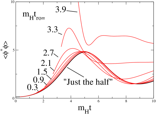
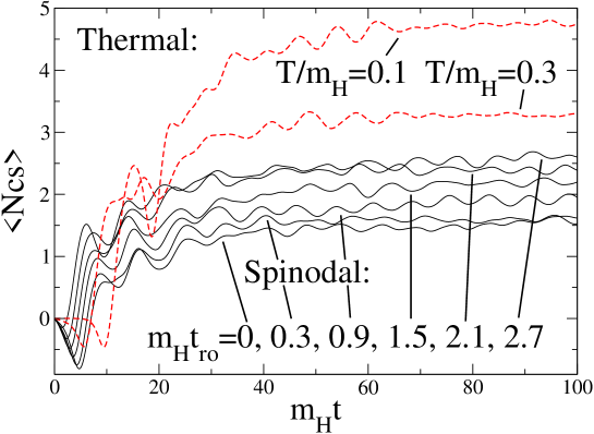
Figure 4: Top: Dependence of $\phi^{\dagger}\phi$ on the roll-off time $t_{\rm ro}$ with ‘spinodal’ initial conditions, including ‘just a half’ ($t_{\rm ro}=0$). The ‘thermal’ case with $T/m_{H}=0.1$ is also shown. Bottom: $\langle N_{cs}\rangle$ in runs with three different initial condition schemes.

5 Numerical results

Most of the results presented here are for a number of lattice points $N=512$, lattice spacing $am_{H}=a\sqrt{2}\mu=0.3$, where $a\equiv a_{1}$, temporal lattice spacing $a_{0}=0.1\,a_{1}$, and volume $Lm_{H}=153.6$. We have typically used an ensemble of 1000 initial conditions and have run for a time $t=600\,m_{H}^{-1}$, keeping track of the average $\langle\phi^{\dagger}\phi\rangle$ and Chern-Simons number, $\langle N_{\rm CS}\rangle$. We studied the dependence on the coupling ratio $2\lambda/e^{2}=m_{H}^{2}/m_{W}^{2}$ and various coupling strengths $\lambda/\mu^{2}=1/8$, …, 1/512. We also checked, using larger lattices ($N=10240$) that the final asymmetry is proportional to the physical volume, $\langle N_{\rm CS}\rangle\propto m_{H}L$.

5.1 Dependence on initial conditions

Figure 4 shows $\langle\phi^{\dagger}\phi\rangle$ and $\langle N_{\rm CS}\rangle$ at early times, for spinodal initial conditions with various choices of the roll-off time $t_{\rm ro}$, and a comparison is made with ‘just a half’ and thermal initial conditions. The $CP$-asymmetry parameter $\kappa=-0.03$. The coupling is fairly weak, $\mu^{2}/\lambda=8$, for which $t_{\rm nl}\approx 1.98$ (from (36) for $\varphi_{1}^{2}=8/3$), with $2\lambda/e^{2}=1$ ($m_{H}=m_{W}$). We see the curves for $\langle\phi^{\dagger}\phi\rangle$ already breaking away from the ‘just a half’ curve for somewhat smaller values of $t_{\rm ro}$ than $t_{\rm nl}$. We have checked that these deviations diminish for weaker couplings. The plot for $\langle N_{\rm CS}\rangle$ contains also a comparison with the thermal method for $T/m_{H}=0.1$ and $0.3$. Compared to the ‘just a half’ curve ($t_{\rm ro}\equiv 0$), the thermal curve has a longer ‘waiting time’ before the initial dip occurs, which indicates smaller fluctuations in the initial conditions. Apparently, the effect of the vacuum fluctuations (characterized by $n_{k}+1/2=1/2$) is substantial in comparison with $n_{k}^{\rm BE}$ at $T/m_{H}=0.1$.

5.2 Initial asymmetry

We can estimate the initial effect of the C and P breaking term from the equations of motion. Approximating the Higgs field by its homogeneous mode falling in the inverted quadratic potential, $\phi(t)=\phi(0)\exp(\mu t)$, inserting this into the equation of motion (7) for $A_{1}$, with $A_{1}(0)=\dot{A}_{1}(0)=0$, neglecting the current-term ($-2e^{2}|\phi|^{2}A_{1}$) and taking into account only the $\kappa$-term, we find at $t=t_{\rm nl}$,

$$A_{1}(t_{\rm nl}=-e^{2}\int_{0}^{t_{\rm nl}}\phi^{*}\phi\,dt\approx\frac{-e^{2}\kappa}{2\mu}\,|\phi(t_{\rm nl})|^{2},$$ (39)

where we have neglected the seed $|\phi(0)|^{2}$ compared to $|\phi(t_{\rm nl})|^{2}$. Using $\phi=(\phi_{1}+i\phi_{2})/\sqrt{2}$ and choosing the 1-axis in the complex plane along $\phi$ (i.e. $\phi_{2}=0$), gives $|\phi(t_{\rm nl})|^{2}=\varphi_{1}^{2}/2=\mu^{2}/6\lambda$ (cf. (36)), and the estimate

$$N_{\rm CS}(t_{\rm nl})=\frac{\kappa}{2\pi}\,\left(\frac{m_{H}}{m_{W}}\right)^{-2}\,\frac{Lm_{H}}{6\sqrt{2}}.$$ (40)

The actual value of the asymmetry in the full simulation in the minimum of the initial dip in $N_{\rm CS}$ in figure 5, is indeed within a factor of two of this estimate (figure 5), and in particular, the sign is right.

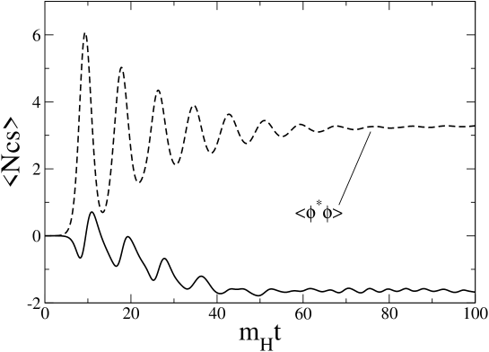
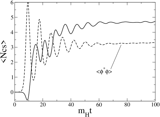
Figure 5: Examples of $\langle N_{\rm CS}\rangle$ for $m_{H}/m_{W}=0.625$ (top) and $1.0625$ (bottom). The volume $Lm_{H}=153.6$ and $\kappa=-0.05$.

5.3 Dependence on $m_{H}/m_{W}$ and $\kappa$

After the initial dip, the behaviour of the Chern-Simons number depends on the ratio of the Higgs to W mass, as shown in figure 5. For $m_{H}/m_{W}$ around 0.625 $\langle N_{\rm CS}\rangle$ keeps the same sign as the initial dip (top plot), for most others it ends up with the opposite sign (bottom plot). The final $N_{\rm CS}$ is typically larger than the value at the bottom of the initial dip due to what looks like resonant behavior.

We end the simulation at a time $m_{H}t=600$ when the trajectories are stuck (see below), and measure the final value of the average Chern-Simons number, $\langle N_{cs}\rangle$. The distribution of the 1000 trajectories in such an average is just gaussian (figure 6).

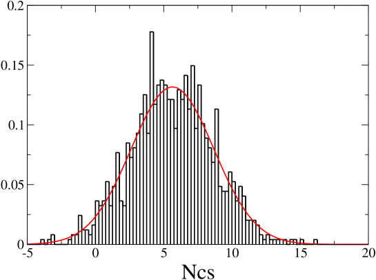
Figure 6: The distribution of the Chern-Simons numbers at $tm_{H}=600$ in an ensemble of 1000 initial conditions. $\kappa=-0.05$, $m_{H}/m_{W}=1.0$.

The dependence of the final Chern-Simons number on the mass ratio $m_{H}/m_{W}$ at fixed $\lambda/\mu^{2}$, $m_{H}L$ and $\kappa$ (so changing $e^{2}$) is quite complicated, see figure 7. Only in a narrow range around $m_{H}/m_{W}=0.6$ is the sign of $\langle N_{\rm CS}\rangle$ the same as that of the initial dip and the input $\kappa$ (negative). For large mass ratio the asymmetry is expected to go down because of the explicit factor $e^{2}$ accompanying $\kappa$ in (7). However, the strong dependence on the mass ratio is related to the resonant behavior mentioned previously.

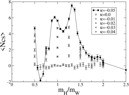
Figure 7: Dependence of the final $\langle N_{\rm CS}\rangle$ on $m_{H}/m_{W}$.

Figure 8: Dependence of the final $\langle N_{\rm CS}\rangle$ on $\kappa$ for $m_{H}/m_{W}=1$.

The actual value of $\kappa$ in realistic models is presumably quite small, so it is comforting to see that the behavior of the final $N_{\rm CS}$ as a function of $\kappa$ is simply linear, see figure 8.

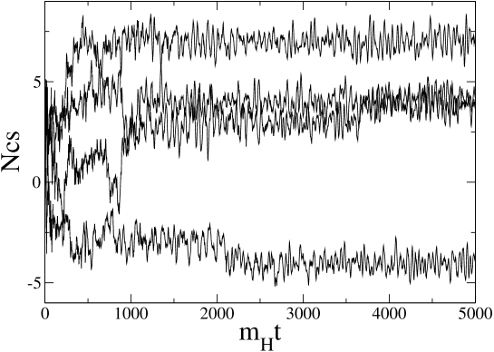
Figure 9: Examples of $N_{\rm CS}$ in single trajectories. $m_{H}/m_{W}=1$.

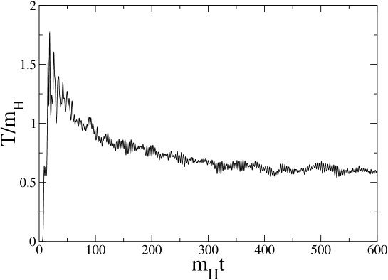
Figure 10: The effective temperature calculated from the canonical momentum of the Chern-Simons degree of freedom.

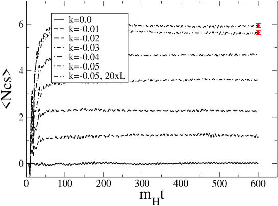
Figure 11: $\langle N_{\rm CS}\rangle$ for different $\kappa$ at $m_{H}/m_{W}=1$, $Lm_{H}=153.6$, except for the top curve, which represents $N_{\rm CS}/20$ in the 20 times larger volume $Lm_{H}=3072$.

5.4 Suppression of sphaleron wash-out

The effective temperature at the end of tachyonic preheating should be low enough that any Chern-Simons asymmetry created by the tachyonic instablility does not get washed out through equilibrium-type sphaleron processes. If the system ends up deep enough in the broken phase the sphaleron rate will be exponentially suppressed with temperature. We can estimate the rate by running single configurations for a long time and monitor effective temperature and transition rate. Figure 9 shows some examples.

The Chern-Simons number eventually gets almost stuck at times of order $1000\,m_{H}^{-1}$ and afterwards the transition rate is strongly suppressed. We estimate the temperature of the system by monitoring the average canonical momentum of the Chern-Simons degree of freedom [28, 29] (this is the only dynamical degree of freedom in the gauge field, as is clear e.g. from the formulation in the Coulomb gauge [29]). A typical evolution of this temperature is shown in Figure 10. For a somewhat different value of $m_{H}/m_{W}$ it was shown in [29] that the sphaleron rate in this model is exponentially suppressed by the sphaleron Boltzmann factor when $\beta^{\prime}\equiv\mu^{3}/(\lambda T)$ is larger than $\simeq 7$. In the case of figure 10 we get $\beta^{\prime}\approx 10$ and so we are deep in the broken phase with a strongly suppressed sphaleron rate. This is also clear from estimates of the rate from pictures like figure 9. When averaging over initial conditions, it turns out that the average Chern-Simons number gets stuck already at $tm_{H}\approx 200$ (fig. 11). Its distribution (fig. 6) then widens at a rate equal to the sphaleron rate.

Of course, in a realistic application the additional degrees of freedom in the Standard Model and the expansion of the universe are expected to lead to further suppression of the rate, such that it ends up being negligible at practically zero temperature.

5.5 Volume dependence

When the volume is increased, the fluctuations of the final Chern-Simons number over the initial ensemble also grow, but the fluctuations in the density $N_{\rm CS}/L$ should go down like $L^{-1/2}$. For a very large volume, one classical realization should suffice to provide an accurate estimate of the density (which in the realistic case would determine the fermion-number density of the universe). We have performed simulations using a 20 times larger volume ($N=10240$, $Lm_{H}=3072$), which should result in an average density that is approximately the same as presented in the previous sections (using $Lm_{H}=153.6$) , with a standard deviation smaller by a factor $\sqrt{20}$. We have checked this by using also 20 times fewer initial conditions ($1000\to 50$), and found the same standard deviation for the density as before. See the upper two curves and their final-time error bars in figure 11 (the top curve represents the largest volume). A closer look revealed that (up to an insignificant shift in time) the two curves are actually indistinguishable until $tm_{H}\approx 13$. Also, the lattice spacing dependence is very small.

Figure 12: Analog of figure 5 in the homogeneous approximation; dashed: $\phi^{2}$ versus $tm_{H}$, continuous: $N_{\rm CS}$. Left: $m_{H}/m_{W}=0.625$, right: $m_{H}/m_{W}=1.0625$. The initial values are $\phi=0.02$, $\dot{\phi}=\dot{A}_{1}=A_{1}=0$.

5.6 Modelling

In this section we attempt to interpret the data in terms of simple models for the dynamics of $N_{\rm CS}$, or equivalently, the homogeneous gauge field in the Coulomb gauge, $A_{1}$. The first model is simply the restriction of the equations of motion to homogeneous fields, with the full non-linear dynamics. Without loss of generality, we can assume $\phi$ to be real. Figure 12 shows the result for parameter values as in figure 5. A striking difference with fig. 5 is the non-linearity of the oscillations in the fields, due to the absence of damping by the in-homogeneous modes. However, it appears that the behavior until the second minumum of $\langle\phi^{*}\phi\rangle$ ($tm_{H}\approx 12$) is reasonably well represented. The initial dips in figure 5 (12) are -0.66 (-0.66) and -0.74 (-0.53), respectively for $m_{H}/m_{W}=0.625$ and 1.0625. In the former case the Chern-Simons number oscillates more rapidly when $\phi^{*}\phi$ is large, because the W mass is larger, and when $\phi^{*}\phi$ is low again after its first maximum, $N_{\rm CS}$ coasts along almost freely in the negative (positive) direction in the left (right) plot of figure 12. The homogeneous approximation breaks clearly down already in the region of the second minimum of $\phi^{*}\phi$, but the sign of the true final asymmetry (fig. 5) is the same as the sign of $N_{\rm CS}$ in this region ($12\lesssim tm_{H}\lesssim 20$) in the homogeneous approximation (fig. 12).

When we add damping terms $\gamma\dot{\phi}$ and $\gamma_{A}\dot{A}_{1}$ to the homogeneous approximation, the resulting $\phi^{2}$ can be made to look pretty much like figure 5, including the oscillation period . However, the resulting $N_{\rm CS}$ then simply performes a damped oscillation around zero. In the real simulations $N_{\rm CS}$ gets stuck in a minimum between the sphaleron energy barriers. We have tried to model this by adding a periodic potential $V_{\rm s}(LA_{1},\phi)$, periodic in $LA_{1}$ with period $2\pi$, and height equal to the sphaleron energy $E_{\rm s}=(2m_{H}/3)v^{2}$, where $v^{2}$ is the expectation value $2\phi^{*}\phi=v^{2}=m_{H}^{2}/2\lambda$ in the classical ground state. The effective action then takes the form

$$S_{\rm eff}=L\int dt\,\left[\frac{\dot{A}_{1}^{2}}{2e^{2}}+\dot{\phi}^{2}+\mu^{2}\phi^{2}-\lambda\phi^{4}+\kappa\dot{A}_{1}\phi^{2}+V(LA_{1},\phi)\right]$$ (41)

Since the homogeneous $\phi$ is varying in time we try the simplistic form $V(LA_{1},\phi)\propto\phi^{2}$:

$$V(LA_{1},\phi)=\phi^{2}L^{-2}f(LA_{1}),$$ (42)

with the tentative conditions

$$f(LA_{1}) = \frac{4}{3}\,m_{H}L,\;\;\;\;LA_{1}=\pi,$$ (43)

$$= (LA_{1})^{2}+O((LA_{1})^{4}),\;\;\;\;LA_{1}\to 0.$$ (44)

The first condition represents the sphaleron energy, the second takes care of the fact that the effective $A_{1}$ mass is $2e^{2}\phi^{2}$. A possible solution can be given in the form $f(LA_{1})=\sum_{n=0}^{2}c_{n}(m_{H}L)\,\cos(nLA_{1})$, with coefficients $c_{n}$ depending on $m_{H}L$. The equations of motion follow straightforwardly from the effective action, after adding also the required damping terms,

$$\ddot{\phi}+\gamma\dot{\phi} = \left(m_{H}^{2}/2-2\lambda\phi^{2}+2L^{-2}f(2\pi N_{\rm CS})+\kappa\dot{A}_{1}\right)\phi,$$ (45)

$$\ddot{N}_{\rm CS}+\tilde{\gamma}e^{2}\dot{N}_{\rm CS} = -(e^{2}/2\pi)\left(f^{\prime}(2\pi N_{\rm CS})\phi^{2}+2\kappa L\phi\dot{\phi}\right)$$ (46)

where we assumed the damping for $A_{1}$ to be proportional to $e^{2}$.

However, for $m_{H}L$ of order 1 (the sphaleron size) and $\kappa=0.05$, the $\kappa$-term is much too small to push the Chern-Simons number over the sphaleron barrier and the resulting asymmetry is zero. For larger volumes the barrier itself is too high to get $N_{\rm CS}$ sufficiently away from zero; the $f^{\prime}$-term in (46) becomes very large near the top of the barrier (cf. (43)). The $f$-term in (45) may actually be neglected for large $L$.

To proceed, we shall interpret the above equations as effective equations for the Chern-Simons density, with an effective potential $f$ that is not constrained by the barrier condition (43), and that is even time-dependent. We have to incorporate the fact that at early times $t\lesssim 13\,m_{H}^{-1}$ the quadratic form $L^{-2}f(LA_{1})=A_{1}^{2}$ gives a reasonable description of the data. The bottom of the dips in figure 12 is deeper than the sphaleron value $-1/2$. This means that the sphalerons have not appeared yet, because $N_{\rm CS}$ bounces back (on the $A_{1}^{2}$ potential) instead of rolling down the hill on the other side of a (lower) sphaleron barrier. We model this by an effective potential that changes from quadratic to periodic, e.g.

$$L^{-2}f(LA_{1}) \to \ell^{-2}[2-2\cos(\ell A_{1})],$$ (47)

$$\ell(t) = \ell_{0}+\ell_{1}[1+\tanh(\delta(t-t_{0}))]/2,$$ (48)

with parameters such that $\ell(t)$ is very small at $t=0$ (and consequently $L^{-2}f(LA_{1})\approx A_{1}^{2}$) and reasonably large at $t=\infty$, such that $A_{1}$ is able to hop over the barrier. For simplicity we set $\ell_{1}=153.6\,m_{H}^{-1}$, the value of $L$ in most figures. Then, with $\ell_{0}=0.01\,m_{H}^{-1}$, $t_{0}=16\,m_{H}^{-1}$, $\delta=0.16\,m_{H}$, and damping coefficients $\gamma=0.14\,m_{H}$, $\tilde{\gamma}=0.8\,m_{H}^{-1}$, we get the result shown in figure 13. The other parameters are as in figure 5 and 12.

Figure 13: Analog of figure 12 including the time-dependent sphaleron-like potential (47,48); dashed: $\phi^{2}$ versus $tm_{H}$, continuous: $N_{\rm CS}$. Left: $m_{H}/m_{W}=0.625$, right: $m_{H}/m_{W}=1.0625$.

Although figure 13 appears to capture the qualitative behavior of the process, we should keep in mind that the model system is quite chaotic, and a small change of e.g. damping coefficients can change the result. This could be avoided by considering an ensemble of initial conditions. The real simulation lacks of course the arbitrary parameters of the modelling, and it is also more subtle, e.g. in that the resonance-like behavior seen in figure 5 is not very well captured by the modelling.

5.7 Role of topological defects

The mechanism proposed in [2, 4] assumed that the electroweak transition produced topological defects in the Higgs field, by the Kibble mechanism, with winding numbers averaging to zero in absence of CP violation. With CP-violating there would then subsequently be a bias towards non-zero average winding number, with a corresponding Chern-Simons number characterizing the vacuum. Translated to our current notation the asymmetry would then be given by a formula of the form $n_{\rm CS}\equiv N_{\rm CS}/L=c\,\kappa\,n_{\rm d}$, where $n_{\rm d}$ is the density of defects and $c$ a dimensionless factor.

However, although we do not doubt the fact that there will be a non-zero density of topological defects shortly after the transition, this does not play a role in our interpretation of the asymmetry as presented in the previous section. With the effective C and P violation used here, the all important initial asymmetry (section 5.2) is already about 10% or more of the final value, and it has nothing to do with the winding-number density of the Higgs field; it depends only on $\kappa\partial_{0}(\phi^{*}\phi)$.

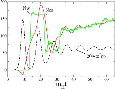
Figure 14: Winding number of the Higgs field $N_{w}$, Chern-Simons number $N_{\rm CS}$ and $\phi^{*}\phi$ in two large-volume ($LmH=3072$) simulations, one with the usual thermal initial conditions (left), and one for which the initial Higgs winding is suppressed (right).

As a check we performed a simulation with initial conditions such, that there is no Kibble mechanism. They were obtained from the thermal initial values by rotating $\phi(x)$ and $\pi(x)$ to the positive real axis, (i.e. $(\mbox{Re}\,\phi,\mbox{Im}\,\phi))\to(|\phi|,0)$, $(\mbox{Re}\,\pi,\mbox{Im}\,\pi))\to(|\pi|,0)$), and subsequently enforcing Gauss’s law. This has the effect that initially there is no topological winding number in the Higgs field. Figure 14 shows an example of the effect on one large-volume configuration, for the $m_{H}=m_{W}$ case. We have also plotted the winding number of the Higgs field.

$$N_{w}=\frac{1}{2\pi}\sum_{x}\left[\alpha(x+a_{1})-\alpha(x)\right]_{-\pi}^{\pi}$$ (49)

with $\phi(x)=\rho(x)e^{i\alpha(x)}$, and where $\left[\ldots\right]_{-\pi}^{\pi}$ denotes taking the value modulo $2\pi$. The artificially non-winding initial configurations are evidently much less random, and we see indeed that $\phi^{*}\phi$ in the right-hand plot of fig. 14 suffers less damping in its first half-period than in the left-hand plot (which resembles closely the corresponding plot in fig. 5). Note also the deeper and broader minimum around $tm_{H}=13$, which reminds us of that in figure 12. However, we note in particular the complete absence of Higgs-winding in the right-hand plot of fig. 14 in $0<tm_{H}<12$, as compared to the somehat noisy winding in this time-interval in the left-hand plot. After time $tm_{H}\simeq 30$, it appears that the Higgs-winding number is pulled along by the Chern-Simons number (bringing down the magnitude of the covariant derivative $D_{1}\phi$), such that in both plots $N_{\rm CS}\approx N_{w}$. Despite the large initial deviations, the final asymmetry is semi-quantitatively unchanged with the artificially winding-suppressing initial conditions.

We conclude that it is the gauge field that, after being biased into the ‘initial dip’, pulls the Higgs phase along, and the picture of a multitude of topological defects un-winding under a biasing C(P) asymmetry in the equations of motion is not relevant for the final asymmetry in the present model.

6 Conclusion

The 1+1 D abelian-Higgs model illustrates nicely that a sizable Chern-Simons asymmetry can be produced by a tachyonic electroweak transition under the influence of the usual effective C- and P-violating interaction. The numerical results can be summarized as

$$n_{\rm CS}=\frac{\langle N_{\rm CS}\rangle}{L}=-0.7\,\kappa\,m_{H},$$ (50)

at $m_{H}/m_{W}=1$ with the dependence on Higgs to W mass ratio as shown in figure 7. The linearity in $\kappa$ enabled us to carry out the simulations at a much larger value than might be expected in realistic applications.

Besides initial conditions that are motivated by the quantum-to-classical transition in the gaussian approximation, we also used low-temperature thermal noise for generating initial configurations. We found that the quantitative results do depend moderately on the choice of initial conditions, but not the qualitative outcome.

It came as a surprise to us that (even the sign of) the final Chern-Simons number and thus the corresponding baryon number asymmetry is very sensitive to the Higgs mass. An interpretation of this intriguing effect was given in section 5.6.

The mechanism for the generation of the asymmetry here is different from that suggested in [1, 2, 4], since neither resonant preheating nor Kibble-like generation of topological defects plays a crucial role in the model studied here.

We have neglected here any effects related to the dynamics of the expansion of the universe, because our primary aim is to see the order of magnitude of the asymmetry that can be generated, given a form of CP violation. It will be very interesting to see similar results in the physically relevant SU(2)-Higgs theory in 3+1 dimension [25].

Appendix A Implementing zero total charge

As discussed in section 4, we need to generate the distribution (35) subject to the constraint of zero total charge, $\sum_{x}e^{2}(\phi^{*}\pi-\pi^{*}\phi)$, or in terms of Fourier variables (defined as in (11)),

$$Q\equiv\sum_{k}\left(\pi_{k}^{1^{*}}\phi_{k}^{2}-\pi_{k}^{2*}\phi_{k}^{1}\right)=0.$$ (51)

On the spatial lattice with an even number of $N$ sites, $x=ma$, $m=0$, …, $N-1$, the wave vectors can be chosen to take the values

$$k=\frac{2\pi n}{Na},\;\;\;\;\;\;n=-N/2+1,...,N/2.$$ (52)

The reality of the fields $\phi^{j}(x)$ and $\pi^{j}(x)$, $j=1,2$, and the fact that $\exp(ikx)$ is real for $n=0$, $N/2$, imply that we can write

$$\phi_{k}^{j} = \phi_{-k}^{j*}=\frac{1}{\sqrt{2\omega_{k}}}\left(a_{k}^{j}+ib_{k}^{j}\right),\;\;\;\;n=1,\ldots,\frac{N}{2}-1,$$ (53)

$$\pi_{k}^{j} = \pi_{-k}^{j*}=\sqrt{\frac{\omega_{k}}{2}}\left(c_{k}^{j}+id_{k}^{j}\right),\;\;\;n=1,\ldots,\frac{N}{2}-1,$$ (54)

$$\phi_{k}^{j} = \frac{1}{\sqrt{\omega_{k}}}\,a^{j}_{k},\;\;\;\;\pi_{k}^{j}=\sqrt{\omega_{k}}\,c^{j}_{k},\;\;\;\;n=0,\;\frac{N}{2},$$ (55)

where the real $a$’s, …, $c$’s, are independent variables. In terms of these the zero-charge condition (51) takes the form

$$Q=c^{1}_{0}a^{2}_{0}-c^{2}_{0}a^{1}_{0}+c^{1}_{N/2}a^{2}_{N/2}-c^{2}_{N/2}a^{1}_{N/2}+\sum_{k=1}^{N/2-1}\left(c^{1}_{k}a^{2}_{k}-c^{2}_{k}a^{1}_{k}+d^{1}_{k}b^{2}_{k}-d^{2}_{k}b^{1}_{k}\right)=0.$$ (56)

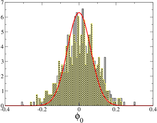
Figure 15: The distribution of (plain) $\phi_{0}^{1}$ (the constrained variable) and of (checkered) $\phi_{0}^{2}$ for a set of 500 initial conditions for a thermal ensemble at temperature $T/m_{H}=0.1$. Overlaid, a gaussian with the relevant width.

To implement the zero charge constraint, the probability distribution (35) has to be multiplied by $\delta(Q(a,b,c,d))$, which means that it no longer depends quadratically on the $a_{k}^{j}$,…, $c_{k}^{j}$. For example, for thermal initial conditions $\tilde{n}_{k}=0$, and we have

$$P(a,b,c,d) \propto \delta(Q)\exp\left[-\frac{1}{2}\sum_{k=1}^{N/2-1}\sum_{j=1}^{2}\left(\frac{a^{j2}_{k}+b^{j2}_{k}+c^{j2}_{k}+d^{j2}_{k}}{n_{k}+1/2}\right)\right.$$ (57)

$$\left.\mbox{}-\frac{1}{2}\sum_{j=1}^{2}\left(\frac{a^{j2}_{0}+c^{j2}_{0}}{n_{0}+1/2}+\frac{a^{j2}_{N/2}+c^{j2}_{N/2}}{n_{N/2}+1/2}\right)\right]$$

We can now integrate out one variable, say $a^{1}_{0}$ to get rid of the $\delta$ function

$$P \to \frac{1}{|c^{2}_{0}|}\exp\left[-\frac{1}{2}\sum_{k,j}\left(\frac{a^{j2}_{k}+b^{j2}_{k}+c^{j2}_{k}+d^{j2}_{k}}{n_{k}+1/2}\right)\right.$$ (58)

$$\left.\mbox{}-\frac{1}{2}\sum_{j}\left(\frac{c^{j2}_{0}}{n_{0}+1/2}+\frac{a^{j2}_{N/2}+c^{j2}_{N/2}}{n_{N/2}+1/2}\right)-\frac{1}{2}\frac{(\tilde{Q}/c^{2}_{0})^{2}}{n_{0}+1/2}\right],$$

where

$$\tilde{Q}(a,b,c,d)=Q(a,b,c,d)+c^{2}_{0}a^{1}_{0}.$$ (59)

This distribution is no longer gaussian in the remaining $a_{k}^{j}$, …, $c_{k}^{j}$. We sample it using Monte-Carlo methods. Sampling a distribution with a $\delta$-function is notoriously difficult. However if we have enough variables on which to “distribute” the constraint, the deviation from a gaussian distribution is expected to be small, which is indeed the case, see figure 15. Our choice of dependent variable ($a_{0}^{1}$) should not matter, in principle, but only with an ideal Monte-Carlo algorithm. As it turned out, the number of variables was sufficiently large that no problem was encountered.

Having produced a realization, we solve for $a^{1}_{0}$ and so construct a field configuration $\{\phi^{j}(x),\pi^{j}(x)\}$ with zero $Q$. As mentioned in section 4, the gauge field configuration then follows from $A_{1}(x)=0$ and determining $\partial_{0}A_{1}(x)$ by solving the Gauss constraint.

- [1] J. García-Bellido, D. Y. Grigoriev, A. Kusenko and M. E. Shaposhnikov, Phys. Rev. D 60 (1999) 123504 [arXiv:hep-ph/9902449].
- [2] L. M. Krauss and M. Trodden, Phys. Rev. Lett. 83 (1999) 1502 [arXiv:hep-ph/9902420].
- [3] J. M. Cornwall, D. Grigoriev and A. Kusenko, Phys. Rev. D 64 (2001) 123518 [arXiv:hep-ph/0106127].
- [4] E. J. Copeland, D. Lyth, A. Rajantie and M. Trodden, Phys. Rev. D 64 (2001) 043506 [arXiv:hep-ph/0103231].
- [5] M. E. Shaposhnikov, Nucl. Phys. B 299 (1988) 797.
- [6] V. A. Rubakov and M. E. Shaposhnikov, Usp. Fiz. Nauk 166 (1996) 493 [Phys. Usp. 39 (1996) 461] [arXiv:hep-ph/9603208].
- [7] D. Y. Grigoriev, M. E. Shaposhnikov and N. Turok, Phys. Lett. B 275 (1992) 395.
- [8] J. Ambjorn, T. Askgaard, H. Porter and M. E. Shaposhnikov, Nucl. Phys. B 353 (1991) 346.
- [9] J. Ambjorn, M. Laursen and M. E. Shaposhnikov, Phys. Lett. B 197 (1987) 49.
- [10] A. D. Linde, Phys. Lett. B 259 (1991) 38.
- [11] G. German, G. Ross and S. Sarkar, Nucl. Phys. B 608 (2001) 423 [arXiv:hep-ph/0103243].
- [12] J. Smit, J. C. Vink and M. Salle, arXiv:hep-ph/0112057. M. Salle, J. Smit and J. C. Vink, Nucl. Phys. Proc. Suppl. 106 (2002) 540 [arXiv:hep-lat/0110093].
- [13] S. Y. Khlebnikov and I. I. Tkachev, Phys. Lett. B 390 (1997) 80.
- [14] S. Y. Khlebnikov and I. I. Tkachev, Phys. Rev. Lett. 79 (1997) 1607.
- [15] S. Y. Khlebnikov and I. I. Tkachev, Phys. Rev. Lett. 77 (1996) 219.
- [16] G. N. Felder, L. Kofman and A. D. Linde, Phys. Rev. D 64 (2001) 123517.
- [17] G. N. Felder, J. Garcia-Bellido, P. B. Greene, L. Kofman, A. D. Linde and I. Tkachev, Phys. Rev. Lett. 87 (2001) 011601.
- [18] G. N. Felder and L. Kofman, Phys. Rev. D 63 (2001) 103503.
- [19] A. Rajantie, P. M. Saffin and E. J. Copeland, Phys. Rev. D 63 (2001) 123512.
- [20] A. Rajantie and E. J. Copeland, Phys. Rev. Lett. 85 (2000) 916.
- [21] G. D. Moore, JHEP 0111 (2001) 021 [arXiv:hep-ph/0109206].
- [22] D. Polarski and A. A. Starobinsky, Class. Quant. Grav. 13 (1996) 377 [arXiv:gr-qc/9504030].
- [23] J. Garcia-Bellido and E. Ruiz Morales, Phys. Lett. B 536 (2002) 193 [arXiv:hep-ph/0109230].
- [24] J. García-Bellido, M. García Pérez and A. González-Arroyo, arXiv:hep-ph/0208228.
- [25] J. Smit and A. Tranberg, arXiv:hep-ph/0210348.
- [26] M. Salle, J. Smit and J. C. Vink, Phys. Rev. D 64 (2001) 025016 [arXiv:hep-ph/0012346].
- [27] G. Aarts and J. Smit, Nucl. Phys. B 511 (1998) 451 [arXiv:hep-ph/9707342].
- [28] A. Krasnitz and R. Potting, Phys. Lett. B 318 (1993) 492 [arXiv:hep-ph/9308307].
- [29] W. H. Tang and J. Smit, Nucl. Phys. B 540 (1999) 437 [arXiv:hep-lat/9805001].
- [30] K. Kajantie, M. Karjalainen, M. Laine, J. Peisa and A. Rajantie, Phys. Lett. B 428 (1998) 334 [arXiv:hep-ph/9803367].