Three-body Baryonic $\overline{B}\to\Lambda\,\bar{p}\,\pi$ Decays and Such

Abstract

We study decay rates and spectra of $\overline{B}\to\Lambda\,\bar{p}\,\pi$, $\Sigma^{0}\,\bar{p}\,\pi$, $\Sigma^{-}\,\bar{n}\,\pi$, $\Xi^{0}\,\overline{\Sigma}{}^{+}\,\pi$, $\Xi^{-}\,\overline{\Sigma}{}^{0}\,\pi$ and $\Xi^{-}\,\overline{\Lambda}\,\pi$ modes under a factorization approach. The baryon pairs are produced through vector, axial vector, scalar and pseudoscalar operators. Previous predictions, including ours, are an order of magnitude too small compared to experiment. By incorporating QCD counting rules and studying the asymptotic behavior, we find an earlier relation between the pseudoscalar and axial vector form factors to be too restrictive. Instead, the pseudoscalar and scalar form factors are related asymptotically. Following this approach, the measured $\Lambda\,\bar{p}\,\pi^{+}$ rate ($\sim 4.0\times 10^{-6}$) and spectrum can be understood, and $\Lambda$ should be dominantly left-hand polarized, while we expect ${\mathcal{B}}(\Sigma^{0}\,\bar{p}\,\pi^{+})\simeq 1.6\times 10^{-6}$. These results and other predictions can be checked soon.

I Introduction

Several three-body baryonic $B$ decays such as $\bar{B}\to D^{*}\,p\,\bar{n}$ Anderson:2000tz , $p\,\bar{p}\,K$ Abe:2002ds and $D^{*}\,p\,\bar{p}$ Abe:2002tw have emerged recently, even though there is only one single two-body baryonic mode $\bar{B}^{0}\to\Lambda^{+}_{c}\,\bar{p}$ that is observed so far Abe:2002er ; Gabyshev:2002dt . It has been argued that three-body baryonic modes could be enhanced over two-body Hou:2000bz , by reducing energy release to the baryons via emitting a fast recoil meson. One consequence is enhancement near baryon pair threshold in three-body modes. In our study of $B^{0}\to D^{*-}\,p\,\bar{n}$ Chua:2001vh , assuming factorization, we obtained $\sim$ 60% of experimental rate from the vector current contribution, and the decay spectrum exhibits such threshold enhancement. The same threshold enhancement effect was predicted for the charmless $\rho\,p\,\bar{n}$ mode Chua:2001xn , and, interestingly, the newly observed first ever charmless baryonic mode, $B\to p\,\bar{p}\,K$, showed similar feature Abe:2002ds . The measured decay rate can be understood to some extent Cheng:2001tr and the spectrum can be reproduced by using the factorization approach and QCD counting rule arguments Chua:2002wn . Other charmless modes such as $p\,\bar{p}\,\pi$, $\Lambda\,\bar{p}\,\pi$, $\Sigma^{0}\,\bar{p}\,\pi$ have been studied under the factorization assumption and ${\mathcal{B}}(\Lambda\,\bar{p}\,\pi^{+})=(3$–$5)\times 10^{-7}$ and ${\mathcal{B}}(\Sigma^{0}\,\bar{p}\,\pi^{+})=(0.8$–$1.8)\times 10^{-6}$ were predicted Cheng:2001tr ; Chua:2002wn .

Recently, Belle reported lambdappi

$${\mathcal{B}}(\Lambda\,\bar{p}\,\pi^{+})=(3.97^{+1.00}_{-0.80}\pm 0.56)\times 10^{-6},$$ (1)

and ${\mathcal{B}}(\Sigma^{0}\,\bar{p}\,\pi^{+})<3.8\times 10^{-6}$ at the 90% confidence level. While the $\Lambda\,\bar{p}\,\pi$ decay spectrum exhibits threshold enhancement as expected, the measured rate turns out to be an order of magnitude higher than predicted Cheng:2001tr ; Chua:2002wn . Furthermore, previous predictions placed ${\mathcal{B}}(\Sigma^{0}\,\bar{p}\,\pi^{+})$ considerably above ${\mathcal{B}}(\Lambda\,\bar{p}\,\pi^{+})$. If the factorization approach is not to be abandoned, where could things go wrong?

We had noted that the $\overline{B}\to\Lambda\,\bar{p}\,\pi^{+}$ mode is sensitive to how one treats the vacuum to $\Lambda\bar{p}$ pseudoscalar matrix element Chua:2002wn under factorization. The analogous situation for meson case is known to be enhanced. In this work, we revisit these two modes, as well as some SU(3) related modes such as $\Sigma^{-}\,\bar{n}\,\pi$, $\Xi^{0}\,\overline{\Sigma}{}^{+}\,\pi$, $\Xi^{-}\,\overline{\Sigma}{}^{0}\,\pi$ and $\Xi^{-}\,\overline{\Lambda}\,\pi$. With the help of QCD counting rules and taking into account the asymptotic behavior of baryonic form factors, we can now account for the observed $\Lambda\,\bar{p}\,\pi$ rate and spectra, where $\Lambda\bar{p}$ production is dominated by the pseudoscalar density. After improving the situation on the $\Lambda\,\bar{p}\,\pi$ rate, we study the $\Lambda$ polarization, which is known to be useful for constructing $CP$- and $T$-violation observables Hou:2000bz . We are able to make some predictions as well.

Our formulation is given in the next section, followed by results and discussion.

II Formalism

Under the factorization assumption, the three-body baryonic $B$ decay amplitude consists of two parts. For one, the baryon pair is current-produced in association with a $B$ to meson transition. For the other, the $B$ makes a transition to a baryon pair and the recoil meson is current-produced Chua:2002wn . The $B\to p\,\bar{p}\,K$ mode receives both contributions, but the $\Lambda\,\bar{p}\,\pi^{+}$ mode, and analogously its SU(3) related modes such as $\Sigma^{0}\,\bar{p}\,\pi^{+}$, $\Sigma^{-}\,\bar{n}\,\pi^{+}$, $\Xi^{0}\,\overline{\Sigma}{}^{+}\,\pi^{+}$, $\Xi^{-}\,\overline{\Sigma}{}^{0}\,\pi^{+}$ and $\Xi^{-}\,\overline{\Lambda}\,\pi^{+}$, receive only the current-produced contribution. We shall apply the term “current-produced” to scalar and pseudoscalar densities as well.

Take, for example, the $\overline{B}{}^{0}\to\Lambda\,\bar{p}\,\pi^{+}$ decay. Under factorization, the amplitude is Chua:2002wn

$${\cal M}(\Lambda\,\bar{p}\,\pi^{+}) = \frac{G_{F}}{\sqrt{2}}\langle\pi^{+}|\bar{u}\gamma^{\mu}(1-\gamma_{5})b|\overline{B}{}^{0}\rangle\bigg{\{}(V_{ub}V_{us}^{*}a_{1}-V_{tb}V_{ts}^{*}a_{4})\langle\Lambda\bar{p}\,|\bar{s}\gamma_{\mu}(1-\gamma_{5})u|0\rangle$$ (2)

$$+2a_{6}V_{tb}V_{ts}^{*}\,\frac{(p_{\Lambda}+p_{\bar{p}})_{\mu}}{m_{b}-m_{u}}\langle\Lambda\bar{p}\,|{\bar{s}(1+\gamma_{5})u}|0\rangle\bigg{\}}.$$

The baryon pair $\Lambda\,\bar{p}$ is produced from vacuum through $\bar{s}\,\gamma_{\mu}\,(\gamma_{5})u$ and $\bar{s}\,(\gamma_{5})u$ operators, while $\overline{B}{}^{0}$ to $\pi^{+}$ transition is induced by $\bar{u}\gamma^{\mu}b$ current. Note that, from isospin symmetry, we have $\langle\pi^{0}|\bar{u}\gamma^{\mu}b|B^{-}\rangle=\langle\pi^{+}|\bar{u}\gamma^{\mu}b|\overline{B}{}^{0}\rangle/\sqrt{2}$, hence ${\cal M}(\Lambda\,\bar{p}\,\pi^{0})={\cal M}(\Lambda\,\bar{p}\,\pi^{+})/\sqrt{2}$. For these current-produced modes, we have

$${\mathcal{B}}(B^{-}\to{\mathbf{B}}\overline{\mathbf{B}}^{\prime}\pi^{0})=\frac{\tau_{B^{-}}}{2\,\tau_{\overline{B}{}^{0}}}\,{\mathcal{B}}(\overline{B}{}^{0}\to{\mathbf{B}}\overline{\mathbf{B}}^{\prime}\pi^{+}),$$ (3)

where $\tau_{\overline{B}{}^{0},\,B^{-}}$ are the $\overline{B}{}^{0}$ and $B^{-}$ meson lifetimes, and ${\mathbf{B}}$ stands for some baryon.

The (axial) vector current-produced matrix elements are decomposed as

$$\langle{\rm\bf B}\overline{\rm\bf B}^{\prime}|V_{\mu}|0\rangle = \bar{u}(p_{\rm\bf B})\left\{(F_{1}+F_{2})\gamma_{\mu}+\frac{\,F_{2}(t)}{m_{\rm\bf B}+m_{{\rm\bf B}^{\prime}}}\left(p_{\overline{\rm\bf B}^{\prime}}-p_{\rm\bf B}\right)_{\mu}\right\}v(p_{\overline{\rm\bf B}^{\prime}})\,,$$ (4)

$$\langle{\rm\bf B}\overline{\rm\bf B}^{\prime}|A_{\mu}|0\rangle = \bar{u}(p_{\rm\bf B})\left\{g_{A}\left(t\right)\gamma_{\mu}+\frac{h_{A}\left(t\right)}{m_{\rm\bf B}+m_{{\rm\bf B}^{\prime}}}\,\left(p_{\rm\bf B}+p_{\overline{\rm\bf B}^{\prime}}\right)_{\mu}\right\}\gamma_{5}\,v(p_{\overline{\rm\bf B}^{\prime}})\,,$$ (5)

where $F_{1,2}$, $g_{A}$ and $h_{A}$ are the induced vector (Dirac and Pauli), axial and the induced pseudoscalar form factors, respectively, and $t\equiv(p_{\rm\bf B}+p_{\overline{\rm\bf B}^{\prime}})^{2}\equiv m^{2}_{{\mathbf{B}}\overline{\mathbf{B}}^{\prime}}$. The scalar and pseudoscalar matrix elements associated with the $a_{6}$ term of Eq. (2) are expressed as

$$\langle{\rm\bf B}\overline{\rm\bf B}^{\prime}|S|0\rangle = f_{S}\left(t\right)\,\bar{u}(p_{\rm\bf B})v(p_{\overline{\rm\bf B}^{\prime}})\,,$$ (6)

$$\langle{\rm\bf B}\overline{\rm\bf B}^{\prime}|P|0\rangle = g_{P}\left(t\right)\,\bar{u}(p_{\rm\bf B})\gamma_{5}\,v(p_{\overline{\rm\bf B}^{\prime}}).$$ (7)

It is the $g_{P}(t)$ form factor that is the focus of our attention, where we offer a refined discussion in face of $B\to\Lambda\,\bar{p}\,\pi^{+}$ data.

The scalar and vector matrix elements can be related by the equation of motion, $\langle{\rm\bf B}\overline{\rm\bf B}^{\prime}|\partial^{\mu}V_{\mu}|0\rangle=i\,(m_{q}-m_{q^{\prime}})\langle{\mathbf{B}}\overline{\mathbf{B}}^{\prime}|\bar{q}\,q^{\prime}|0\rangle$, giving Cheng:2001tr ; Chua:2002wn

$$f_{S}(t)=\frac{m_{\rm\bf B}-m_{{\rm\bf B}^{\prime}}}{m_{q}-m_{q^{\prime}}}\,F_{1}(t).$$ (8)

We note that it is safe in the chiral limit $m_{q}$, $m_{q^{\prime}}\to 0$, and for $m_{q}\to m_{q^{\prime}}$ as well. For example, for $\langle\Lambda\bar{p}|\bar{s}u|0\rangle$ we have $({m_{\Lambda}-m_{p}})/({m_{s}-m_{u}})\sim 1$. For the modes studied here, the factor $({m_{\rm\bf B}-m_{{\rm\bf B}^{\prime}}})/(m_{s}-m_{u})$ varies by $30,\,40\%$, which illustrates SU(3) breaking.

The pseudoscalar and axial current matrix elements can be analogously related. Using $\langle{\rm\bf B}\overline{\rm\bf B}^{\prime}|\partial^{\mu}A_{\mu}|0\rangle=(m_{q}+m_{q^{\prime}})\langle{\mathbf{B}}\overline{\mathbf{B}}^{\prime}|\bar{q}\,i\,\gamma_{5}\,q^{\prime}|0\rangle$, we have

$$g_{A}(t)+\frac{t}{(m_{\rm\bf B}+m_{{\rm\bf B}^{\prime}})^{2}}\,h_{A}(t)=\frac{m_{q}+m_{q^{\prime}}}{m_{\mathbf{B}}+m_{{\mathbf{B}}^{\prime}}}\,g_{P}(t).$$ (9)

As $m_{q},\,m_{q^{\prime}}\to 0$, we get $h_{A}(t)\to-g_{A}(t)\,(m_{\mathbf{B}}+m_{{\mathbf{B}}^{\prime}})^{2}/t$  Cheng:2001tr . Since the $m_{q}/m_{\mathbf{B}}$ ratio is small, one is close to the chiral limit, hence the dependence of $h_{A}(t)$ on $g_{P}(t)$ is weak. However, to ensure good chiral behavior, we previously followed Ref. Cheng:2001tr and took Chua:2002wn

$$g_{P}(t)=-g_{A}(t)\,\frac{m^{2}_{\rm GB}(m_{\mathbf{B}}+m_{{\mathbf{B}}^{\prime}})}{(m_{q}+m_{q^{\prime}})(t-m^{2}_{\rm GB})},$$ (10)

where $m_{\rm GB}$ is the corresponding Goldstone boson (e.g. kaon) mass. That is, $g_{P}(t)$ is obtained by changing the $1/t$ term in the asymptotic form of $h_{A}(t)$ to $1/(t-m^{2}_{\rm GB})$ and make use of Eq. (9) Cheng:2001tr . Indeed, Eq. (10) gave too small a rate for $B\to\Lambda\,\bar{p}\,\pi^{+}$ Cheng:2001tr ; Chua:2002wn . Due to the small quark-baryon mass ratio in Eq. (9), we note that $g_{A}$ and $h_{A}$ are insensitive to $g_{P}$. Therefore in the previous approach we need a very precise information on both $g_{A}$ and $h_{A}$, which is unavailable so far, to pinpoint $g_{P}$. In this work we choose a different strategy by studying $g_{A,P}$ directly and obtaining $h_{A}$ through Eq. (9).

According to QCD counting rules Brodsky:1974vy , both the vector form factor $F_{1}$ and the axial form factor $g_{A}$, supplemented by leading logs, behave as $1/t^{2}$ in the $t\to\infty$ limit. This is because we need two hard gluons to impart large momentum transfer. Similarly, considering the bilinear structure of the $S$ and $P$ operators, the scalar form factor $f_{S}$ and pseudoscalar form factor $g_{P}$ also behave as $1/t^{2}$ in the asymptotic limit. However, due to the need for helicity flip, one needs an extra $1/t$ for $F_{2}$ and $h_{A}$, hence they behave as $1/t^{3}$. We see that Eq. (10) gives $1/t^{3}$ rather than $1/t^{2}$ asymptotic behavior for $g_{P}$, which is symptomatic. In the electromagnetic current case, the asymptotic form has been confirmed by many experimental measurements of the nucleon magnetic form factor $G^{p,n}_{M}=F^{p,n}_{1}+F^{p,n}_{2}$, over a wide range of momentum transfers in the space-like region. The asymptotic behavior for $G^{p}_{M}$ also seems to hold in the time-like region, as reported by the Fermilab E760 experiment Armstrong93 for $8.9$ GeV${}^{2}<t<13$ GeV². Another Fermilab experiment, E835, has recently reported Ambrogiani:1999bh $G^{p}_{M}$ for momentum transfers up to $\sim 14.4$ GeV². An empirical fit of $\left|G^{p}_{M}\right|=Ct^{-2}[\ln({t}/{Q_{0}^{2}})]^{-2}$ is obtained, which is in agreement with the QCD counting rule.

Table 1: Relations of baryon form factors $F_{1}+F_{2}$, $g_{A}$ and $g_{P}$ with the nucleon magnetic form factors $G_{M}^{p,n}$, $D_{A,P}$ and $F_{A,P}$ via the $(\bar{s}u)_{V,A,P}$ operators. Replacing $G^{p,n}_{M}$ by $G^{p,n}_{E}$ in the second column, one obtains $F_{1}+F_{2}\,t/(m_{\mathbf{B}}+m_{\overline{\mathbf{B}}^{\prime}})^{2}$.

${\mathbf{B}}\overline{\mathbf{B}}^{\prime}$	$F_{1}+F_{2}$	$g_{A,\,P}$
$\Lambda\,\bar{p}$	$-\sqrt{\frac{3}{2}}\,G^{p}_{M}$	$-\frac{1}{\sqrt{6}}\left(D+3F\right)_{A,P}$
$\Sigma^{0}\,\bar{p}$	$\frac{-1}{\sqrt{2}}\left(G_{M}^{p}+2\,G_{M}^{n}\right)$	$\frac{1}{\sqrt{2}}\,\left(D-F\right)_{A,P}$
$\Sigma^{-}\,\bar{n}$	$-(G^{p}_{M}+2\,G^{n}_{M})$	$(D-F)_{A,P}$
$\Xi^{0}\,\overline{\Sigma}{}^{+}$	$G^{p}_{M}-G^{n}_{M}$	$(D+F)_{A,P}$
$\Xi^{-}\,\overline{\Sigma}{}^{0}$	$\frac{1}{\sqrt{2}}\,\left(G^{p}_{M}-G^{n}_{M}\right)$	$\frac{1}{\sqrt{2}}\,\left(D+F\right)_{A,P}$
$\Xi^{-}\,\overline{\Lambda}$	$\sqrt{\frac{3}{2}}\,\left(G^{p}_{M}+G^{n}_{M}\right)$	$-\frac{1}{\sqrt{6}}\left(D-3F\right)_{A,P}$

The current induced form factors $F_{1}$, $F_{2}$ for the modes studied here can be related to the nucleon (Sachs) magnetic and electric form factors $G_{M,E}$, as shown in Table 1, where we also give the SU(3) decomposition of $g_{A}$ and $g_{P}$ in terms of the form factors $D_{A,P}$ and $F_{A,P}$. The $F_{1}+F_{2}$ terms are in fact obtained by using

$$D_{V}=-\frac{3}{2}\,G^{n}_{M},\qquad F_{V}=G^{p}_{M}+\frac{1}{2}\,G^{n}_{M},$$ (11)

with SU(3) decompositions similar to that of $g_{A,P}$. We can decompose $f_{S}$ similarly into $D_{S}$ and $F_{S}$, with (compare Eq. (8))

$$D_{S}=\frac{m_{\rm\bf B}-m_{{\rm\bf B}^{\prime}}}{m_{q}-m_{q^{\prime}}}\,\left(-\frac{3}{2}\,F^{n}_{1}\right),\qquad F_{S}=\frac{m_{\rm\bf B}-m_{{\rm\bf B}^{\prime}}}{m_{q}-m_{q^{\prime}}}\,\left(F^{p}_{1}+\frac{1}{2}\,F^{n}_{1}\right).$$ (12)

From the factorization assumption and Table 1, we expect

$${\mathcal{B}}(\Lambda\,\bar{p}\,\pi^{+})\sim 2\,{\mathcal{B}}(\Lambda\,\bar{p}\,\pi^{0}),$$

$${\mathcal{B}}(\Sigma^{-}\,{\bar{n}}\,\pi^{+})\sim 2\,{\mathcal{B}}(\Sigma^{-}\,{\bar{n}}\,\pi^{0})\sim 2\,{\mathcal{B}}(\Sigma^{0}\,\bar{p}\,\pi^{+})\sim 4\,{\mathcal{B}}(\Sigma^{0}\,\bar{p}\,\pi^{0}),$$

$${\mathcal{B}}(\Xi^{0}\,\overline{\Sigma}{}^{+}\,\pi^{+})\sim 2\,{\mathcal{B}}(\Xi^{0}\,\overline{\Sigma}{}^{+}\,\pi^{0})\sim 2\,{\mathcal{B}}(\Xi^{-}\,\overline{\Sigma}{}^{0}\,\pi^{+})\sim 4\,{\mathcal{B}}(\Xi^{-}\,\overline{\Sigma}{}^{0}\,\pi^{0}).$$ (13)

There is considerable data on the nucleon magnetic form factors. This allows us to make a fit Chua:2001vh :

$$G_{M}^{p}(t)=\sum^{5}_{i=1}\frac{x_{i}}{t^{i+1}}\left[\ln\left(\frac{t}{\Lambda_{0}^{2}}\right)\right]^{-\gamma},G_{M}^{n}(t)=-\sum^{2}_{i=1}\frac{y_{i}}{t^{i+1}}\left[\ln\left(\frac{t}{\Lambda_{0}^{2}}\right)\right]^{-\gamma},$$ (14)

where $\gamma=2.148$, $x_{1}=420.96$ GeV⁴, $x_{2}=-10485.50$ GeV⁶, $x_{3}=106390.97$ GeV⁸, $x_{4}=-433916.61$ GeV¹⁰, $x_{5}=613780.15$ GeV¹², $y_{1}=292.62$ GeV⁴, $y_{2}=-735.73$ GeV⁶, and $\Lambda_{0}=0.3$ GeV. They satisfy QCD counting rules and describe time-like electromagnetic data such as $e^{+}e^{-}\to N\overline{N}$ suitably well. The data is extracted by assuming $|G^{p}_{E}|=|G^{p}_{M}|$ and $|G^{n}_{E}|=0$ (which gives better fit compared to the $|G^{n}_{E}|=|G^{n}_{M}|$ case Antonelli:fv ). With the fit of Eq. (14), time-like $G^{p\,(n)}_{M}$ is real and positive (negative) Mergell:1996bf ; Baldini:1999qn . It is interesting to note that the fit coefficients $x_{i}$s alternate in sign, and likewise for $y_{i}$s. Just two terms suffice for the latter because the neutron magnetic form factor data is relatively sparse Chua:2001vh . According to perturbative QCD Lepage:1979za , asymptotically ($t\to\infty$) one expects $G^{n}_{M}/G^{p}_{M}=-2/3$. We find that the fitted parameters for $G_{M}^{n}$ with the $|G^{n}_{E}|=0$ assumption gives $G^{n}_{M}/G^{p}_{M}\rightarrow-y_{1}/x_{1}=-0.70$, which is within 5% of the QCD expectation. Note that, by use of $G_{M}=F_{1}+F_{2}$ and asymptotically $F_{2}/F_{1}\to 1/t\to 0$, we have $F^{n}_{1}/F^{p}_{1}\to G^{n}_{M}/G^{p}_{M}\to-2/3$ as well.

The $F_{2}$ term can be related to $(G_{E}-G_{M})/[t/(m_{\bf B}+m_{\bf B^{\prime}})^{2}-1]$. However, we do not have much data on time-like nucleon $G_{E}$. Thus, we concentrate on the $F_{1}+F_{2}$ term in Eq. (4) as we did in Refs. Chua:2001vh ; Chua:2002wn . We also use $G_{M}$ in place of $F_{1}$ in Eqs. (8) and (12). The effect of the $F_{2}$ (or equivalently $G_{E}-G_{M}$) contribution can be estimated by using form factor models such as Vector Meson Dominance (VMD), where both $G_{E}$ and $G_{M}$ are available.

The time-like form factors related to $D_{A}$, $F_{A}$ are not yet measured, but, as pointed out in Ref. Cheng:2001tr , their asymptotic behavior at $t\to\infty$ are known Brodsky:1980sx and useful. Asymptotically, they can be described by two form factors, depending on the reacting quark having parallel or anti-parallel spin with respect to the baryon spin Brodsky:1980sx . By expressing these two form factors in terms of $G_{M}^{p,n}$ as $t\to\infty$, one has

$$D_{A}\to G_{M}^{p}+\frac{3}{2}\,G_{M}^{n},\qquad F_{A}\to\frac{2}{3}\,G_{M}^{p}-\frac{1}{2}\,G_{M}^{n}.$$ (15)

In similar fashion, in the asymptotic region the $f_{S}$ and $g_{P}$ form factors for the chirality flip operators $S$ and $P$ can be expressed by just one form factor, with spin of the interacting quark parallel to the baryon spin. Anti-parallel spin corresponds to an octet-decuplet instead of an octet-octet baryon pair. Since $g_{P}$ (equivalently $D_{P},\ F_{P}$) and $f_{S}$ are related to the same form factor, by following the approach of Ref. Brodsky:1980sx , as shown in Appendix A, we have

$$g_{P}\to f_{S},\qquad\frac{D_{P(S)}}{F_{P(S)}}\to\frac{3}{2},$$ (16)

as $t\to\infty$. This is a non-trivial requirement and it is not obeyed by Eq. (10). We note that Eq. (16) is obtained without the use of the equation of motion. The requirement of $D_{S}/F_{S}\to 3/2$ is consistent with Eq. (12), which follows from Eq. (8) by using $F^{n}_{1}/F^{p}_{1}\to G_{M}^{n}/G_{M}^{p}\to-2/3$ asymptotically Lepage:1979za . Thus, the use of the equation of motion for $f_{S}$ in Eq. (8) is consistent with the asymptotic relations in Eq. (16).

The asymptotic relations hold for large $t$, hence they imply relations on the leading terms of the corresponding form factors. In general, more terms would be needed. In analogy to the neutron magnetic form factor case, we express $D_{A,P}$, $F_{A,P}$ up to the second term Chua:2002wn ,

$$D_{A}(t) \equiv \left(\frac{\tilde{d}_{1}}{t^{2}}+\frac{\tilde{d}_{2}}{t^{3}}\right)\left[\ln\left(\frac{t}{\Lambda_{0}^{2}}\right)\right]^{-\gamma},$$

$$F_{A}(t) \equiv \left(\frac{\tilde{f}_{1}}{t^{2}}+\frac{\tilde{f}_{2}}{t^{3}}\right)\left[\ln\left(\frac{t}{\Lambda_{0}^{2}}\right)\right]^{-\gamma},$$

$$D_{P}(t) \equiv \left(\frac{\bar{d}_{1}}{t^{2}}+\frac{\bar{d}_{2}}{t^{3}}\right)\left[\ln\left(\frac{t}{\Lambda_{0}^{2}}\right)\right]^{-\gamma},$$

$$F_{P}(t) \equiv \left(\frac{\bar{f}_{1}}{t^{2}}+\frac{\bar{f}_{2}}{t^{3}}\right)\left[\ln\left(\frac{t}{\Lambda_{0}^{2}}\right)\right]^{-\gamma}.$$ (17)

The asymptotic relations of Eqs. (15), (16) imply $\tilde{d}_{1}=x_{1}-3\,y_{1}/2$, $\tilde{f}_{1}=2\,x_{1}/3+y_{1}/2$, $\bar{d}_{1}=(3y_{1}/2)[(m_{\rm\bf B}-m_{{\rm\bf B}^{\prime}})/(m_{q}-m_{q^{\prime}})]$ and $\bar{f}_{1}=(x_{1}-y_{1}/2)[(m_{\rm\bf B}-m_{{\rm\bf B}^{\prime}})/(m_{q}-m_{q^{\prime}})]$, while further information is needed to determine $\tilde{d}_{2}$, $\tilde{f}_{2}$, $\bar{d}_{2}$ and $\bar{d}_{2}$, as we will discuss in the next section. We note that the anomalous dimensions of $g_{P}$ and $f_{S}$ may not be the same as that of $F_{1,2}$ and $g_{A}$. However, their effect is logarithmic hence not very important, and we apply the anomalous dimension of $F_{1}$ to others for simplicity.

It is useful to compare with Refs. Chua:2002wn ; Cheng:2001tr on the treatment of $g_{P}(t)$ (or equivalently on $h_{A}(t)$), namely Eq. (10). As a working assumption, this form of $g_{P}(t)$ with $m_{\rm GB}^{2}/(m_{q}+m_{q^{\prime}})$ factor was useful in particular for the good behavior of the pseudoscalar matrix element in the chiral limit. However, it may be too restrictive in three aspects: $g_{P}(t)\propto g_{A}(t)$, which is too strong an assumption; the appearance of the Goldstone boson pole in time-like form factors, although $m_{\rm GB}$ is way below baryon pair threshold; and a $1/t^{3}$ asymptotic behavior, rather than the $1/t^{2}$ form as expected from QCD counting rules. Ultimately, it does not satisfy the asymptotic relation of Eq. (16). We have improved on these points in our present treatment of $g_{P}(t)$.

III Results

It is straightforward to use Eq. (2) to calculate $B\to\Lambda\,\bar{p}\,\pi$ and similar rates. Before we start, let us first specify the parameters used. We take $\phi_{3}$ (or $\gamma$) $=60^{\circ}$ Ciuchini:2000de and central values of $|V_{cb}|$ and $|V_{ub}|$ from Ref. PDG . We use $m_{u(d)}/m_{s}=0.029\,(0.053)$, $m_{s}=120$ MeV and $m_{b}=4.88$ GeV at $\mu=2.5$ GeV PDG ; Leutwyler:1996qg . The $B\to\pi$ transition form factor is given in Ref. Melikhov:2000yu . For effective Wilson coefficients, we use $a_{1}=1.05$, $a_{4}\times 10^{4}=-387.3-121i$ and $a_{6}\times 10^{4}=-555.3-121i$ from Ref. Cheng:1999xj with $N_{c}=3$.

Following Ref. Chua:2002wn , we use the axial vector contribution to $B^{0}\rightarrow D^{*-}\,p\,\bar{n}$ decay to constrain $\tilde{f}_{2}$ and $\tilde{d}_{2}$. Since there is no scalar and pseudoscalar contribution in this tree dominated mode, we simply use the chiral limit form of $h_{A}(t)=-g_{A}(t)\,(m_{p}+m_{n})^{2}/t$. The $g_{P}$ contribution is suppressed by the quark-baryon mass ratio. We update our previous calculation Chua:2001vh using the present input parameters, finding the vector part of the branching ratio to be ${\mathcal{B}}_{V}(D^{*-}\,p\,\bar{n})=11.9\,(a^{\rm eff}_{1}/0.85)^{2}\times 10^{-4}$, where the same $a^{\rm eff}_{1}$ value as in Ref. Cheng:2002fp is used. To reach the central value of the measured rate ${\cal B}(B^{0}\to D^{*-}\,p\,\bar{n})=(14.5^{+3.4}_{-3.0}\pm 2.7)\times 10^{-4}$ Anderson:2000tz , using $\tilde{d}_{2}+\tilde{f}_{2}=-956\,{\rm GeV}^{6}$ correction , we find ${\cal B}_{A}(D^{*-}\,p\,\bar{n})=2.6\,(a^{\rm eff}_{1}/0.85)^{2}\times 10^{-4}$ from the axial current. Although the value of $\tilde{d}_{2}+\tilde{f}_{2}$ is about half of what was used in Refs. Chua:2002wn and Cheng:2002fp , the change only affects the branching ratios of the charmless modes studied here at the $10^{-8}$ level. Following Ref. Chua:2002wn , we use $\tilde{d}_{2}=\tilde{f}_{2}$.

With the axial contribution fixed, and with the scalar and vector contribution related by the equation of motion (Eq. (12)) we give in Table 2, the vector plus scalar contribution (${\mathcal{B}}_{V}$) and the axial plus pseudoscalar contribution (${\mathcal{B}}_{A}$) to $\overline{B}{}^{0}\to{\mathbf{B}}\overline{\mathbf{B}}^{\prime}\pi^{+}$ branching ratios. For ${\mathcal{B}}_{A}$, we show two cases with either vanishing or non-vanishing $\bar{d}_{2}$ and $\bar{f}_{2}$ from the pseudoscalar form factor, which is yet to be fixed. Since the contribution from the vector plus scalar part does not interfere with the axial plus pseudoscalar part, the branching fraction is a simple sum of the two, i.e. ${\mathcal{B}}={\mathcal{B}}_{V}+{\mathcal{B}}_{A}$, just as for $B^{0}\rightarrow D^{*-}\,p\,\bar{n}$. By using the relation of Eq. (3), ${\mathcal{B}}({\mathbf{B}}\overline{\mathbf{B}}^{\prime}\pi^{0})$ can be read off from Table 2 by a simple 1/2 factor.

Table 2: Branching fractions for ${\mathbf{B}}\overline{\mathbf{B}}^{\prime}\pi^{+}$ modes arising from the vector and scalar parts (${\mathcal{B}}_{V}$), and from the axial and pseudoscalar parts (${\mathcal{B}}_{A}$). The latter are given for the two cases of using the asymptotic $g_{P}$ ($\bar{d}_{2}=\bar{f}_{2}=0$) or the fitted $g_{P}$ ($\bar{d}_{2}=\bar{f}_{2}=-952\,{\rm GeV}^{6}$) from the $\Lambda\,\bar{p}\,\pi$ rate. The branching fraction is a simple sum of the two, i.e. ${\mathcal{B}}={\mathcal{B}}_{V}+{\mathcal{B}}_{A}$. Rates for ${\mathbf{B}}\overline{\mathbf{B}}^{\prime}\pi^{0}$ modes are about one half of those shown.

Modes	${\mathcal{B}}_{V}(10^{-6})$	${\mathcal{B}}_{A}(10^{-6})$
		use asymptotic $g_{P}$	use fitted $g_{P}$
$\Lambda\,\bar{p}\,\pi^{+}$	$0.13$	$7.97$	$3.84$
$\Sigma^{0}\,\bar{p}\,\pi^{+}$	$0.88$	$0.70$	$0.70$
$\Sigma^{-}\,\bar{n}\,\pi^{+}$	$1.79$	$1.41$	$1.41$
$\Xi^{0}\,\overline{\Sigma^{+}}\,\pi^{+}$	$0.17$	$2.23$	$1.20$
$\Xi^{-}\,\overline{\Sigma^{0}}\,\pi^{+}$	$0.09$	$1.14$	$0.63$
$\Xi^{-}\,\overline{\Lambda}\,\pi^{+}$	$0.15$	$0.38$	$0.20$

We find ${\mathcal{B}}_{V}(\Lambda[\Sigma^{0}]\,\bar{p}\,\pi^{+})=0.13\,[0.88]\times 10^{-6}$. We note that ${\mathcal{B}}_{V}(\Lambda\,\bar{p}\,\pi^{+})$ is consistent with previous studies Chua:2002wn ; Cheng:2001tr , while ${\mathcal{B}}_{V}(\Sigma^{0}\,\bar{p}\,\pi^{+})$ becomes slightly larger because of the different input values of the neutron magnetic form factor parameters ($y_{i}$s). Clearly, ${\mathcal{B}}_{V}(\Lambda\,\bar{p}\,\pi^{+})$ part is still an order of magnitude below the measured lambdappi branching ratio of Eq. (1). Before invoking the pseudoscalar form factor of Eq. (17), let us make sure that other modifications are insufficient for the order of magnitude difference.

Recall that in the vector and scalar sector, we concentrated on $F_{1}+F_{2}$ contributions without including the $G_{E}-G_{M}$ effect since $G_{E}$ data is unavailable. As noted earlier, one can try to estimate the $G_{E}-G_{M}$ effect by using some form factor model where both $G_{E}$ and $G_{M}$ are given. We use a VMD model, Ref. Mergell:1996bf , which was discussed in our previous work Chua:2001vh . Since $F^{\Lambda\bar{p}}_{1}(t)$ and $F^{\Lambda\bar{p}}_{2}(t)$ can be expressed in terms of $G_{M}^{p}$ and $G^{p}_{E}$, and since the VMD model describes $G_{M}^{p}$ data better than $G_{M}^{n}$ (time-like) data Mergell:1996bf , perhaps the $\Lambda\,\bar{p}\,\pi^{+}$ mode may be a better place to estimate the $G_{E}-G_{M}$ effect. By incorporating VMD with the previous section (following similar approach of Ref. Chua:2001vh ), we obtain ${\mathcal{B}}_{V}(\Lambda\,\bar{p}\,\pi^{+})=0.27\times 10^{-6}$. Although we gain by a factor of two compared to Table 2, the effect is still of order $10^{-7}$, and is insufficient to account for the measured $\Lambda\,\bar{p}\,\pi^{+}$ rate. The effect of $G_{E}-G_{M}$ is not likely to fill the gap between ${\mathcal{B}}_{V}(\Lambda\,\bar{p}\,\pi^{+})$ and the measured ${\mathcal{B}}(\Lambda\,\bar{p}\,\pi^{+})$.

We thus need to turn to the axial and pseudoscalar contributions. Let us start by using only the $\bar{d}_{1}$ and $\bar{f}_{1}$ terms of $g_{P}$ determined by the asymptotic relation of Eq. (16), i.e. taking $\bar{d}_{2}=\bar{f}_{2}=0$. It is remarkable that, as given in the first case for ${\mathcal{B}}_{A}$ in Table 2 (column three), the $1/t^{2}$ terms of $D_{P}$ and $F_{P}$ alone give ${\mathcal{B}}(\Lambda\,\bar{p}\,\pi^{+})\sim 8\times 10^{-6}$, or overshooting the experimental value by a factor of two! This is striking compared with the previous calculation using the ansatz of Eq. (10), which gave results an order of magnitude too small Chua:2002wn ; Cheng:2001tr . Now, we know that the sign of $x_{i}$s and $y_{i}$s alternate hence $G_{M}$ gets reduced as higher power (in $1/t$) terms are included. We expect similar effect for $g_{P}$ by allowing for nonzero $\bar{d}_{2}$ and $\bar{f}_{2}$. We determine these coefficients (the $1/t^{3}$ terms) by fitting to the central value of the measured $\Lambda\,\bar{p}\,\pi^{+}$ rate. We obtain $-(\bar{d}_{2}+3\,\bar{f}_{2})/\sqrt{6}=1554.6\,{\rm GeV}^{6}$, which is displayed as the second case for ${\mathcal{B}}_{A}$ in Table 2. By assuming $\bar{d}_{2}\sim\bar{f}_{2}$, we have $\bar{d}_{2}\sim-952\ {\rm GeV}^{6}$, which has sign opposite to $\bar{d}_{1}$, and is about twice the size of $\tilde{d}_{2}=\tilde{f}_{2}=-478\,{\rm GeV}^{6}$, the $1/t^{3}$ coefficients for the axial vector form factor.

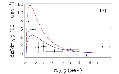
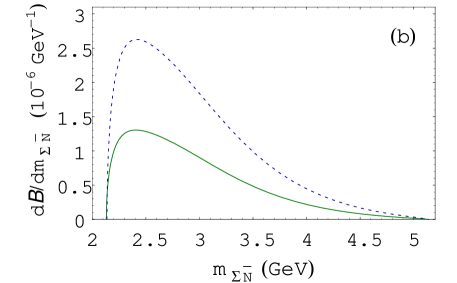
Figure 1: (a) $d{\mathcal{B}}(\Lambda\,\bar{p}\,\pi^{+})/dm_{\Lambda\bar{p}}$ spectrum, where solid (dashed) line is for using the fitted (asymptotic) $g_{P}$ of $\bar{d}_{2}=\bar{f}_{2}=-952\,{\rm GeV}^{6}\,(0)$; (b) $d{\mathcal{B}}(\Sigma\,\bar{N}\,\pi^{+})/dm_{\Sigma\bar{N}}$ spectra, where solid (dotted) line is for $\Sigma^{0}\bar{p}$ ($\Sigma^{-}\bar{n}$). The plots for $\pi^{+}$ replaced by $\pi^{0}$ are expected to be similar but factor of 2 lower.

We show in Fig. 1(a) the $\Lambda\,\bar{p}\,\pi^{+}$ decay spectrum. It is interesting that the predicted spectra in both $\bar{d}_{2}=\bar{f}_{2}=0$ and $\bar{d}_{2}=\bar{f}_{2}=-952\,{\rm GeV}^{6}$ cases are close to data. The data suggests a curve between these two, which conforms with our expectation that the third, $1/t^{4}$ term would have same sign as $1/t^{2}$ term. In future as the measured spectrum improved, one may in turn use it to extract baryon time-like from factors.

While ${\mathcal{B}}(\Lambda\,\bar{p}\,\pi^{+})$ is enhanced from the previous results Chua:2002wn ; Cheng:2001tr by using our new approach to pseudoscalar $g_{P}$ form factor, the enhancement in ${\mathcal{B}}(\Sigma^{0}\,\bar{p}\,\pi^{+})$ turns out to be rather mild. This can be understood from the relative weight of $\Lambda$ vs. $\Sigma^{0}$ in Eq. (23) of Appendix A. We expect ${\mathcal{B}}(\Sigma^{0}\,\bar{p}\,\pi^{+})=1.6\times 10^{-6}$, which is within the present Belle limit of ${\mathcal{B}}(\Sigma^{0}\,\bar{p}\,\pi^{+})<3.8\times 10^{-6}$ at 90% confidence level lambdappi . Furthermore, it is easy to verify the SU(3) predictions of ${\mathcal{B}}(\Sigma^{-}\,{\bar{n}}\,\pi^{+})\sim 2\,{\mathcal{B}}(\Sigma^{0}\,\bar{p}\,\pi^{+})$ and ${\mathcal{B}}(\Xi^{0}\,\overline{\Sigma}{}^{+}\,\pi^{+})\sim 2\,{\mathcal{B}}(\Xi^{-}\,\overline{\Sigma}{}^{0}\,\pi^{+})$ given in Table 2.

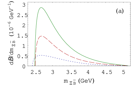
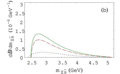
Figure 2: Solid, dashed and dotted lines are for $d{\mathcal{B}}(\Xi^{0}\,\overline{\Sigma^{+}}\,\pi^{+})/dm_{\Xi^{0}\,\overline{\Sigma^{+}}}$, $d{\mathcal{B}}(\Xi^{-}\,\overline{\Sigma^{0}}\,\pi^{+})/dm_{\Xi^{-}\,\overline{\Sigma^{0}}}$ and $d{\mathcal{B}}(\Xi^{-}\,\overline{\Lambda}\,\pi^{+})/dm_{\Xi^{-}\,\overline{\Lambda}}$, respectively, for using (a) the asymptotic $g_{P}$ ($\bar{d}_{2}=\bar{f}_{2}=0$), and (b) the fitted $g_{P}$ ($\bar{d}_{2}=\bar{f}_{2}=-952\,{\rm GeV}^{6}$).

In Fig. 1(b) we plot the $\Sigma^{0}\,\bar{p}\,\pi^{+}$ and $\Sigma^{-}\,\bar{n}\,\pi^{+}$ decay spectra. The $\Sigma^{0}\,\bar{p}\,\pi^{+}$ spectrum is close to our previous calculation in Ref. Chua:2002wn . Since the corresponding SU(3) decomposition for these two mode is $D_{P}-F_{P}$, the rates are not sensitive to $\bar{d}_{2}$ and $\bar{f}_{2}$ being zero or finite, so long that they are not too different from each other. We show in Fig. 2 the $\Xi^{0}\,\overline{\Sigma^{+}}\,\pi^{+}$, $\Xi^{-}\,\overline{\Sigma^{0}}\,\pi^{+}$ and $\Xi^{-}\,\overline{\Lambda}\,\pi^{+}$ decay spectra with $\bar{d}_{2}$ and $\bar{f}_{2}$ zero or finite.

We expect Figs. 1 and 2 to give also the spectra of modes with $\pi^{+}$ replaced by $\pi^{0}$, but with a factor of two reduction in rate from isospin factor.

In these three-body modes quite often we have a $\Lambda$ hyperon produced, which is well known to self-analyse its spin upon decay and provides useful information for possible $CP$- and $T$-violation and chirality studies in $B$ decays Hou:2000bz ; Suzuki:2002cp . Following Ref. Suzuki:2002cp , the angular distribution of the cascade $\overline{B}\to\Lambda\,\bar{p}\,\pi\to\pi^{-}\,p\,\bar{p}\,\pi$ decay can be written as

$$\frac{d^{2}\Gamma}{dE_{\Lambda}d\cos\theta}=\frac{1}{2}\frac{d\Gamma}{dE_{\Lambda}}[1+\overline{\alpha}_{\Lambda}(E_{\Lambda})\cos\theta],$$ (18)

where $E_{\Lambda}$ is the $\Lambda$ energy measured in the $\overline{B}$ rest frame and $\theta$ is the supplementary angle between the emitted proton momentum and the $\overline{B}$ momentum in the $\Lambda$ rest frame. We have $\overline{\alpha}_{\Lambda}(E_{\Lambda})={\cal P}_{\Lambda}(E_{\Lambda})\,\alpha_{\Lambda}$, where the $\Lambda$ polarization ${\cal P}_{\Lambda}(E_{\Lambda})$ is given in Appendix B and the $\alpha_{\Lambda}=0.642\pm 0.013$ PDG is the well-measured $\Lambda$ decay asymmetry parameter.

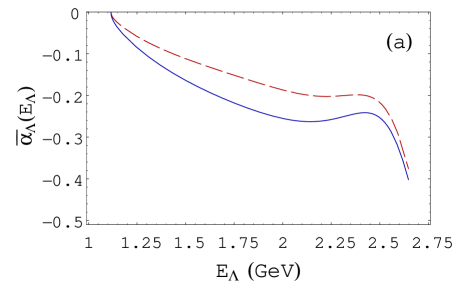
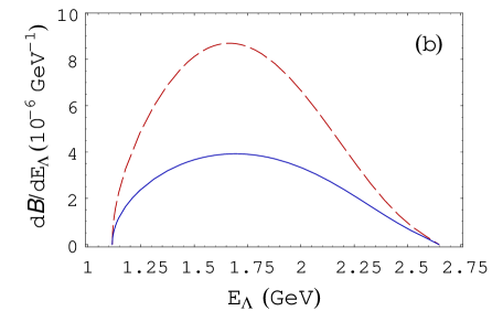
Figure 3: (a) $\overline{\alpha}_{\Lambda}(E_{\Lambda})$, (b) $d{\mathcal{B}}(\Lambda\,\bar{p}\,\pi^{+})/dE_{\Lambda}$ spectrum, where solid (dashed) line is for using the fitted (asymptotic) $g_{P}$ of $\bar{d}_{2}=\bar{f}_{2}=-952\,{\rm GeV}^{6}\,(0)$.

We show in Fig. 3 the asymmetry $\overline{\alpha}_{\Lambda}(E_{\Lambda})$ and $d{\mathcal{B}}(\Lambda\,\bar{p}\,\pi^{+})/dE_{\Lambda}$ spectrum. The $\overline{\alpha}_{\Lambda}(E_{\Lambda})$ plot is similar to the plot shown in Ref. Suzuki:2002cp obtained by using some general arguments. The negative $\overline{\alpha}_{\Lambda}(E_{\Lambda})$ corresponds to a left-handed helicity dominated $\Lambda$ in $B$ decay. It is interesting to note that although the decay rate is dominated by the pseudoscalar term, we still have polarized $\Lambda$. This can be understood by noting that the ratio of scalar and pseudoscalar contributions is roughly given by the averaged $f^{2}_{S}/g_{P}^{2}$, which is about 0.1, while the polarization ${\cal P}_{\Lambda}$ is roughly given by the averaged $-2f_{S}\,g_{P}/(f_{S}^{2}+g_{P}^{2})\sim-2f_{S}/g_{P}$ which can be as large as $-0.6$. The sharp turn of $\overline{\alpha}_{\Lambda}(E_{\Lambda})$ towards much negative value for $E_{\Lambda}>2.5$ GeV is due to the fact that as $E_{\Lambda}$ increases, phase space quickly reduces to a high $m_{\Lambda\bar{p}}$ region, resulting in the approach of $g_{P}$ to $f_{S}$ and consequently the increase in left-handed $\Lambda$ polarization. It is well known that the $\Lambda$ spin is mainly carried by the $s$ quark (as shown in Eq. (A2)) and it is left-handed in the $\overline{B}\to\Lambda\,\bar{p}\,\pi$ decay (as shown in Eq. (2)). Therefore, a dominantly left-handed $\Lambda$ reflects the $V-A$ nature of the weak interaction Suzuki:2002cp . By comparing Fig. 3(a) and Fig. 3(b), we find $-\overline{\alpha}_{\Lambda}\sim 0.2$–$0.3$ for the main portion of $\Lambda\,\bar{p}\,\pi$ events. One should be able to check the sign of this asymmetry experimentally in the near future.

IV Discussion and Conclusion

Let us check the $\phi_{3}$ dependence of the modes considered here. For all modes, ${\mathcal{B}}_{V}$ increases as we change $\phi_{3}$ from $60^{\circ}$ to $90^{\circ}$; on the other hand, ${\mathcal{B}}_{A}$ increases for $\Lambda\,\bar{p}\,\pi$, $\Sigma\,\overline{N}\,\pi$ and $\Xi^{-}\,\overline{\Lambda}\,\pi$, but decreases for $\Xi^{0}\,\overline{\Sigma}^{+}\,\pi$ and $\Xi^{-}\,\overline{\Sigma}^{0}\,\pi$. However, the variations are at $10^{-7}$ order and far less significant compared to the $K\pi$ case He:1999mn . Since $a_{6}\,V_{tb}\,V_{ts}^{*}$ terms dominate, we do not expect strong dependence on $\phi_{3}$ or $N_{c}$. Similarly, single term dominance implies direct CP violation cannot be large, which are found to be within $+5$% for all modes.

It is interesting to discuss the implication on $p\,\bar{p}\,K$ and $p\,\bar{p}\,\pi$ modes calculated in Ref. Cheng:2001tr ; Chua:2002wn . First of all, the changes are in the current-produced parts, whereas these modes contain transition parts as well. In particular, the $p\,\bar{p}\,\pi^{-}$ mode is dominated by transition. From Eq. (9), we see that $h_{A}(t)$ is close to its chiral limit form because the dependence on $g_{P}$ is rather weak, and $h_{A}(t)$ for the present work is similar to previous Cheng:2001tr ; Chua:2002wn . Therefore, the axial vector contributions to $p\,\bar{p}\,K$ and $p\,\bar{p}\,\pi$ modes are not affected. The effect of $g_{P}$ only enter through the pseudoscalar term. Since the pseudoscalar matrix element for $B\to p\,\bar{p}\,K$ decay, $\langle p\bar{p}\,|(\bar{s}s)_{P}|0\rangle$ Chua:2002wn , is Okubo-Zweig-Iizuka (OZI) suppressed, we do not expect much change in these modes. On the other hand, for $\langle p\bar{p}\,|(\bar{d}d)_{P}|0\rangle$ of the $p\,\bar{p}\,\pi^{-}$ mode, by using SU(3) and OZI argument as in Ref. Chua:2002wn , corresponds to $F_{P}-D_{P}$ and is non-negligible. However, this mode is tree and transition dominant, hence we still do not expect much change in rate Chua:2002wn . Note that the transition form factor has a $1/t^{3}$ behavior. For large enough $t$, the transition part is power suppressed. We thus expect to see some $1/t^{2}$ contribution from the new $g_{P}$ term, resulting in a slightly broader spectrum than previous Chua:2002wn .

In conclusion, we study decay rates and spectra of $\overline{B}\to\Lambda\,\bar{p}\,\pi$, $\Sigma^{0}\,\bar{p}\,\pi$, $\Sigma^{-}\,\bar{n}\,\pi$, $\Xi^{0}\,\overline{\Sigma}{}^{+}\,\pi$, $\Xi^{-}\,\overline{\Sigma}{}^{0}\,\pi$ and $\Xi^{-}\,\overline{\Lambda}\,\pi$ modes, and the $\Lambda$ polarization in this work. By suitably incorporating the asymptotic behavior of the baryonic pseudoscalar matrix element, we are able to obtain the $\Lambda\,\bar{p}\,\pi^{+}$ rate (in part by a fit) and spectrum close to experimental measurements. The discrepancy between experimental lambdappi and previous theoretical Cheng:2001tr ; Chua:2002wn results is perhaps resolved. While the $\Lambda\,{\bar{p}}\,\pi^{+}$ rate is enhanced from the previous calculation, we expect ${\mathcal{B}}(\Sigma^{0}\,\bar{p}\,\pi^{+})=1.6\times 10^{-6}$, which is within the present experimental limit and can be checked soon. Although the $\Lambda\,\bar{p}\,\pi^{+}$ rate is dominated by the pseudoscalar term, we still have $\Lambda$ polarized giving $\overline{\alpha}_{\Lambda}\sim-(0.2$–$0.3)$. The impact on $p\,\bar{p}\,K$ due to the present treatment of the pseudoscalar form factor is negligible, while we expect a slight broadening of the $p\,\bar{p}\,\pi^{-}$ spectrum. Most of the subtleties in these modes come from the axial and especially the pseudoscalar form factors. Information on these form factors may be obtained from studying these modes. However, the underlying factorization assumption needs to be checked separately. It is interesting that factorization seems to work in $\overline{B}^{0}\to D^{+}K^{-}K^{0}$ and $D^{*+}K^{-}K^{0}$ modes, where axial parts are absent and vector parts are known Chua:2002pi . For these current-produced three-body baryonic modes, we expect ${\mathcal{B}}({\mathbf{B}}\overline{\mathbf{B}}^{\prime}\pi^{+})\sim 2\,{\mathcal{B}}({\mathbf{B}}\overline{\mathbf{B}}^{\prime}\pi^{0})$ as a consequence of factorization, which does not depend on the complexity of baryonic form factors.

Appendix A Asymptotic relations for form factors $f_{S}$ and $g_{P}$

We follow Ref. Brodsky:1980sx to obtain the asymptotic relations for $f_{S}$ and $g_{P}$. The wave function of an octet baryon can be expressed as

$$|{\mathbf{B}}\,;\uparrow\rangle\sim\frac{1}{\sqrt{3}}(|{\mathbf{B}}\,;\uparrow\downarrow\uparrow\rangle+|{\mathbf{B}}\,;\uparrow\uparrow\downarrow\rangle+|{\mathbf{B}}\,;\downarrow\uparrow\uparrow\rangle),$$ (19)

i.e. composed of 13-, 12- and 23-symmetric terms, respectively. For ${\mathbf{B}}=p,\,n,\,\Sigma^{0},\,\Lambda$, we have

$$|p\,;\uparrow\downarrow\uparrow\rangle = \left[\frac{d(1)u(3)+u(1)d(3)}{\sqrt{6}}u(2)-\sqrt{\frac{2}{3}}u(1)d(2)u(3)\right]|\uparrow\downarrow\uparrow\rangle,$$

$$|n\,;\uparrow\downarrow\uparrow\rangle = (-|p\,;\uparrow\downarrow\uparrow\rangle\,\,{\rm with}\,\,u\leftrightarrow d),$$

$$|\Sigma^{0}\,;\uparrow\downarrow\uparrow\rangle = \bigg{[}-\frac{u(1)d(3)+d(1)u(3)}{\sqrt{3}}\,s(2)+\frac{u(2)d(3)+d(2)u(3)}{2\sqrt{3}}\,s(1)$$

$$\,\,+\frac{u(1)d(2)+d(1)u(2)}{2\sqrt{3}}\,s(3)\bigg{]}|\uparrow\downarrow\uparrow\rangle,$$

$$|\Lambda\,;\uparrow\downarrow\uparrow\rangle = \bigg{[}\frac{d(2)u(3)-u(2)d(3)}{2}\,s(1)+\frac{u(1)d(2)-d(1)u(2)}{2}\,s(3)\bigg{]}|\uparrow\downarrow\uparrow\rangle,$$ (20)

for the corresponding $|{\mathbf{B}}\,;\uparrow\downarrow\uparrow\rangle$ parts, while the 12- and 23-symmetric parts can be obtained by permutation. To be consistent with the SU(3) decompositions of Table I, our $\Lambda$ state has an overall negative sign with respect to that of Ref. Brodsky:1980sx .

Following Ref. Brodsky:1980sx , we have

$$\langle{\mathbf{B}}(p)|{\cal O}|{\mathbf{B}}^{\prime}(p^{\prime})\rangle = \bar{u}(p)\left[\frac{1+\gamma_{5}}{2}\,F^{+}(t)+\frac{1-\gamma_{5}}{2}\,F^{-}(t)\right]u(p^{\prime}),$$

$$F^{\pm}(t) = e^{(\pm)}_{\parallel}({\cal O}:{\mathbf{B}}^{\prime}\to{\mathbf{B}})\,F_{\parallel}(t),$$ (21)

in the large $t$ limit. Quark mass dependent terms behave like $m_{q}/\sqrt{|t|}$ and are neglected. For simplicity, we illustrate with the space-like case. Coefficients of $F_{\parallel}$ for the ${\mathcal{O}}=\bar{q}_{L}q^{\prime}_{R},\,\bar{q}_{L}q^{\prime}_{R}$ cases are given by

$$e^{+}_{\parallel}(\bar{q}_{L}q^{\prime}_{R}:{\mathbf{B}}^{\prime}\to{\mathbf{B}}) = \langle{\mathbf{B}};\,\downarrow\downarrow\uparrow|Q[q^{\prime}(1,\uparrow)\to q(1,\downarrow)]|{\mathbf{B}}^{\prime}\,;\uparrow\downarrow\uparrow\rangle$$

$$+\langle{\mathbf{B}};\,\uparrow\downarrow\downarrow|Q[q^{\prime}(3,\uparrow)\to q(3,\downarrow)]|{\mathbf{B}}^{\prime}\,;\uparrow\downarrow\uparrow\rangle,$$

$$e^{-}_{\parallel}(\bar{q}_{L}q^{\prime}_{R}:{\mathbf{B}}^{\prime}\to{\mathbf{B}}) = 0,$$

$$e^{\pm}_{\parallel}(\bar{q}_{R}q^{\prime}_{L}:{\mathbf{B}}^{\prime}\to{\mathbf{B}}) = e^{\mp}_{\parallel}(\bar{q}_{L}q^{\prime}_{R}:{\mathbf{B}}^{\prime}\to{\mathbf{B}}),$$ (22)

where $Q[q^{\prime}(1(3),\uparrow)\to q(1(3),\downarrow)]$ change the parallel spin $q^{\prime}(1(3))|\uparrow\rangle$ part of $|{\mathbf{B}}^{\prime};\uparrow\downarrow\uparrow\rangle$ to a $q(1(3))|\downarrow\rangle$ part. It is easy to see that flipping the anti-parallel spin $|\downarrow\rangle$ part of $|{\mathbf{B}}^{\prime};\uparrow\downarrow\uparrow\rangle$ to $|\uparrow\rangle$ will give a decuplet instead of an octet state. Thus, we need to consider the parallel spin case only. By using the above equations, it is straightforward to obtain

$$e^{+}_{\parallel}(\bar{u}_{L}d_{R}:n\to p) = -\frac{5}{3},$$

$$e^{+}_{\parallel}(\bar{u}_{L}s_{R}:\Lambda\to p) = \sqrt{\frac{3}{2}},$$

$$e^{+}_{\parallel}(\bar{u}_{L}s_{R}:\Sigma^{0}\to p) = -\frac{1}{3\sqrt{2}}.$$ (23)

By using $S,P=\bar{q}_{L}q^{\prime}_{R}\pm\bar{q}_{R}q^{\prime}_{L}$ and Eq. (22), we have $e^{\pm}_{\parallel}(\bar{q}q^{\prime}:{\mathbf{B}}^{\prime}\to{\mathbf{B}})=e^{+}_{\parallel}(\bar{q}_{L}q^{\prime}_{R}:{\mathbf{B}}^{\prime}\to{\mathbf{B}})$ and $e^{\pm}_{\parallel}(\bar{q}\gamma_{5}q^{\prime}:{\mathbf{B}}^{\prime}\to{\mathbf{B}})=\pm e^{+}_{\parallel}(\bar{q}_{L}q^{\prime}_{R}:{\mathbf{B}}^{\prime}\to{\mathbf{B}})$. Hence

$$f_{S}=g_{P}=e^{+}_{\parallel}(\bar{q}_{L}q^{\prime}_{R}:{\mathbf{B}}^{\prime}\to{\mathbf{B}})\,F_{\parallel},$$ (24)

in the large $t$ limit. In terms of $D_{S(P)}$ and $F_{S(P)}$, we have $f_{S}(g_{P})=D_{S(P)}+F_{S(P)}$, $-(D_{S(P)}+3F_{S(P)})/\sqrt{6}$, $(D_{S(P)}-F_{S(P)})/\sqrt{2}$ for ${\mathbf{B}}^{\prime}{\mathbf{B}}=np$, $\Lambda p$ and $\Sigma^{0}p$ cases, respectively. Accordingly,

$$D_{S}=D_{P}=-F_{\parallel}\,,\qquad F_{S}=F_{P}=-\frac{2}{3}\,F_{\parallel}\,,$$ (25)

which implies Eq. (16).

Appendix B decay rate and polarization formula

For a three-body $B\to h{\rm\bf B}\overline{\rm\bf B}^{\prime}$ decay, where $h$ is a pseudoscalar meson and ${\mathbf{B}}$, $\overline{\mathbf{B}}^{\prime}$ is a baryon anti-baryon pair, in general the amplitude can be written as

$${\cal M}\left(B\to h{\rm\bf B}\overline{\rm\bf B}^{\prime}\right) = \frac{G_{F}}{\sqrt{2}}\,\biggl{\{}{\cal A}\,\bar{u}(p_{{\mathbf{B}}})\,/\!\!\!p_{h}v(p_{\overline{\mathbf{B}}^{\prime}})+{\mathcal{B}}\,\bar{u}(p_{{\mathbf{B}}})\,/\!\!\!p_{h}\gamma_{5}v(p_{\overline{\mathbf{B}}^{\prime}})$$ (26)

$$\qquad\qquad+\,{\cal C}\,\bar{u}(p_{{\mathbf{B}}})v(p_{\overline{\mathbf{B}}^{\prime}})+{\cal D}\,\bar{u}(p_{{\mathbf{B}}})\gamma_{5}v(p_{\overline{\mathbf{B}}^{\prime}})\biggr{\}}\,.$$

The decay rate is given by

$$d\Gamma=\frac{1}{\left(2\,\pi\right)^{3}}\,\frac{1}{32\,m_{B}^{3}}\left(\Sigma_{\lambda_{1,2}}\,\left|{\cal M}\right|^{2}\right)dm_{12}^{2}\,dm_{23}^{2}\,,$$ (27)

where we assign the baryon $\mathbf{B}$ as particle 1, the anti-baryon $\overline{\mathbf{B}}^{\prime}$ as particle 2 and the meson $h$ as particle 3, and $\lambda_{1(2)}=\pm 1$ the helicity of the (anti-)baryon $\mathbf{B}$ ($\overline{\mathbf{B}}^{\prime}$).

If the baryon $\mathbf{B}$ is in a definite helicity state, its spin direction will remain the same in either the $B$ meson or its own rest frames. For the baryon $\mathbf{B}$ with energy $E_{1}$ (measured in the $B$ meson rest frame) the density matrix in the spin (or helicity) space is given by

$$\rho(E_{1})=\frac{1}{2}\left[1+{\cal P}_{\mathbf{B}}(E_{1})\,\hat{p}_{1}\cdot\sigma\right],$$ (28)

where $\hat{p}_{1}$ is the unit vector pointing opposite to the direction of the $B$ meson momentum in the $\mathbf{B}$ baryon rest frame and

$${\cal P}_{\mathbf{B}}(E_{1})=\frac{\int dm^{2}_{23}\,\Sigma_{\lambda_{1,2}}(-)^{\lambda_{1}}|{\cal M}|^{2}}{\int dm^{2}_{23}\,\Sigma_{\lambda_{1,2}}|{\cal M}|^{2}}.$$ (29)

It is straightforward to obtain:

$$\Sigma_{\lambda_{1,2}}\,(-)^{\lambda_{1}}\left|{\cal M}\right|^{2} = G_{F}^{2}\,4\biggl{\{}{\rm Re}({\cal A}\,{\cal B}^{*})m_{1}\bigl{(}2s_{1}\cdot p_{3}\,p_{2}\cdot p_{3}-m_{3}^{2}\,s_{1}\cdot p_{2}\bigr{)}$$ (30)

$$+{\rm Re}\left({\cal A}\,{\cal D}^{*}-{\cal B}\,{\cal C}^{*}\right)m_{1}m_{2}\,s_{1}\cdot p_{3}$$

$$+{\rm Re}\left({\cal A}\,{\cal D}^{*}+{\cal B}\,{\cal C}^{*}\right)\bigl{(}s_{1}\cdot p_{3}\,p_{1}\cdot p_{2}-s_{1}\cdot p_{2}\,p_{1}\cdot p_{3}\bigr{)}$$

$$-{\rm Re}\left({\cal C}\,{\cal D}^{*}\right)m_{1}\,s_{1}\cdot p_{2}\biggr{\}},$$

$$\Sigma_{\lambda_{1,2}}\,\left|{\cal M}\right|^{2} = G_{F}^{2}\,2\biggl{\{}\biggl{[}\left|{\cal A}\right|^{2}\bigl{(}2p_{1}\cdot p_{3}\,p_{2}\cdot p_{3}-m_{3}^{2}\,p_{1}\cdot p_{2}-m_{1}m_{2}m_{3}^{2}\bigr{)}$$ (31)

$$+2\,{\rm Re}\left({\cal A}\,{\cal C}^{*}\right)\bigl{(}m_{1}p_{2}\cdot p_{3}-m_{2}\,p_{1}\cdot p_{3}\bigr{)}+\bigl{|}{\cal C}\bigr{|}^{2}\bigl{(}p_{1}\cdot p_{2}-m_{1}m_{2}\bigr{)}\biggr{]}$$

$$+\biggl{[}{\cal A}\to{\cal B},\,{\cal C}\to{\cal D},\,m_{2}\to-m_{2}\biggl{]}\biggr{\}}\,,$$

where $s_{1}$ is the helicity vector of the baryon $\mathbf{B}$ (spinor) with $\lambda_{1}=+1$. It is easy to check that by neglecting $m_{1}$ we have $m_{1}s_{1}\to p_{1}$ and we obtain ${\cal P}_{\mathbf{B}}(E_{1})\to-1$ in the fully left-handed chiral case (${\cal A}\sim-{\cal B}$ and ${\cal C}\sim{\cal D}$) as expected from Eq. (26). In general, the polarization ${\cal P}_{\mathbf{B}}(E_{1})$ can be easily evaluated in the $B$ meson rest frame by using

$$s_{1}=\frac{1}{m_{1}\sqrt{(p_{B}\cdot p_{1})^{2}-m_{1}^{2}m_{B}^{2}}}(p_{B}\cdot p_{1}\,p_{1}-m_{1}^{2}\,p_{B}),$$ (32)

where $p_{B}$ is the momentum of the $B$ meson, and the standard technique of expressing $p_{B}\cdot p_{i}$, $p_{i}\cdot p_{j}$ in terms of $m^{2}_{ij}$. Given these formulas, the task is now reduced to extract the ${\cal A}$–${\cal D}$ terms for an amplitude of interest.

References

(1)
S. Anderson et al. [CLEO Collaboration],
Phys. Rev. Lett. 86, 2732 (2001)
[hep-ex/0009011].
(2)
K. Abe et al. [Belle Collaboration],
Phys. Rev. Lett. 88, 181803 (2002)
[hep-ex/0202017].
(3)
K. Abe et al. [Belle Collaboration],
Phys. Rev. Lett. 89, 151802 (2002)
[hep-ex/0205083].
(4)
K. Abe et al. [Belle Collaboration],
Phys. Rev. D 65, 091103 (2002)
[hep-ex/0203027].
(5)
N. Gabyshev and H. Kichimi et al. [Belle Collaboration],
hep-ex/0212052.
(6)
W.S. Hou and A. Soni,
Phys. Rev. Lett. 86, 4247 (2001)
[hep-ph/0008079].
(7)
C.K. Chua, W.S. Hou and S.Y. Tsai,
Phys. Rev. D 65, 034003 (2002)
[hep-ph/0107110].
(8)
C.K. Chua, W.S. Hou and S.Y. Tsai,
Phys. Lett. B 528, 233 (2002)
[hep-ph/0108068].
(9)
H.Y. Cheng and K.C. Yang,
Phys. Rev. D 66, 014020 (2002)
[hep-ph/0112245].
(10)
C.K. Chua, W.S. Hou and S.Y. Tsai,
Phys. Rev. D 66, 054004 (2002)
[hep-ph/0204185].
(11)
K. Abe et al. [Belle Collaboration],
BELLE-CONF-0237;
hep-ex/0302024.
(12)
S.J. Brodsky and G.R. Farrar,
Phys. Rev. D 11, 1309 (1975).
(13) T.A. Armstrong et al. [E760 Collaboration],
Phys. Rev. Lett. 70, 1212 (1993).
(14)
M. Ambrogiani et al. [E835 Collaboration],
Phys. Rev. D 60, 032002 (1999).
(15)
A. Antonelli et al.,
Nucl. Phys. B 517, 3 (1998).
(16)
P. Mergell, U.-G. Meissner and D. Drechsel,
Nucl. Phys. A 596, 367 (1996) [hep-ph/9506375],
H.W. Hammer, U.-G. Meissner and D. Drechsel,
Phys. Lett. B 385, 343 (1996) [hep-ph/9604294].
(17)
R. Baldini et al.,
Eur. Phys. J. C 11, 709 (1999).
(18)
G.P. Lepage and S.J. Brodsky,
Phys. Rev. Lett. 43, 545 (1979)
[Erratum-ibid. 43, 1625 (1979)].
(19)
S.J. Brodsky, G.P. Lepage and S.A. Zaidi,
Phys. Rev. D 23, 1152 (1981).
(20)
M. Ciuchini et al.,
JHEP 0107, 013 (2001)
[hep-ph/0012308].
(21)
K. Hagiwara et al. [Particle Data Group Collaboration],
Phys. Rev. D 66, 010001 (2002).
(22)
H. Leutwyler,
Phys. Lett. B 378, 313 (1996)
[hep-ph/9602366].
(23)
D. Melikhov and B. Stech,
Phys. Rev. D 62, 014006 (2000)
[hep-ph/0001113].
(24)
H.Y. Cheng and K.C. Yang,
Phys. Rev. D 62, 054029 (2000)
[hep-ph/9910291].
(25)
H.Y. Cheng and K.C. Yang,
Phys. Rev. D 66, 094009 (2002)
[hep-ph/0208185].
(26)
By correcting a code error in Ref Chua:2002wn , we can reproduce
Ref. Cheng:2002fp result
by using their value
determinded form the rate.
We do not use the mode to fit form factor parameters,
since it is more complicated than the mode.
(27)
M. Suzuki,
hep-ph/0208060.
(28)
X.G. He, W.S. Hou and K.C. Yang,
Phys. Rev. Lett. 83, 1100 (1999)
[hep-ph/9902256];
W.S. Hou and K.C. Yang,
Phys. Rev. D 61, 073014 (2000)
[hep-ph/9908202];
W.S. Hou, J.G. Smith and F. Wurthwein,
hep-ex/9910014.
(29)
C.K. Chua, W.S. Hou, S.Y. Shiau and S.Y. Tsai,
Phys. Rev. D 67, 034012 (2003)
[hep-ph/0209164].