Lepton flavor violation in lopsided models
and a neutrino mass model

Abstract

A widely adopted theoretical scheme to account for the neutrino oscillation phenomena is the see-saw mechanism together with the “lopsided” mass matrices, which is generally realized in the framework of supersymmetric grand unification. We will show that this scheme leads to large lepton flavor violation at low energy if supersymmetry is broken at the GUT or Plank scale. Especially, the branching ratio of $\mu\to e\gamma$ already exceeds the present experimental limit. We then propose a phenomenological model, which can account for the LMA solution to the solar neutrino problem and at the same time predict branching ratio of $\mu\to e\gamma$ below the present limit.

I see-saw mechanism and “lopsided” structure

The neutrino experiments show that the neutrino parameters have two exotic while interesting features, i.e., the extreme smallness of the neutrino masses and the large size of the neutrino mixing anglessk ; k2k ; sno . According to the recent analyses the atmospheric neutrino oscillation favors the $\nu_{\mu}-\nu_{\tau}$ process with the best fit valuesatm

$$\Delta m^{2}_{atm}=2.5\times 10^{-3}eV^{2},\ \ \sin^{2}2\theta_{atm}=1.$$ (1)

Among the four oscillation solutions for the solar neutrino problem, the large mixing angle MSW (LMA) solution is most favored, followed by the LOW and VAC solutionssma ; lma ; bahcall . The best fit values for the LMA solution arebahcall

$$\Delta m^{2}_{sol}=5\times 10^{-5}eV^{2},\ \ \tan^{2}\theta_{sol}=0.42.$$ (2)

The same analysis excludes the small mixing angle (SMA) solution at 3.7 $\sigma$ level.

On the theoretical side, hundreds of neutrino mass models have been constructed in the literaturebarr , each trying to explain to a greater or lesser degree the two afore-mentioned features. A consensus has now emerged that the see-saw mechanism seems to be the most natural and economical way to account for the tiny neutrino masses.

In the see-saw mechanism, the Standard Model (SM) is extended by including the right-handed Majorana neutrinos, $\nu_{R}$. Since $\nu_{R}$ are the SM gauge group, $SU(2)_{W}\times U(1)_{Y}$, singlets, their masses are not protected by the SM gauge symmetry. The $\nu_{R}$ may get masses at very high energy scale and may be much heavier than the SM particles. Having both left- and right-handed neutrinos and the $\nu_{R}$ being singlets, the neutrinos can have both Dirac mass terms,

$${\cal L}_{D}=-M_{D}\bar{\nu}_{L}\nu_{R}+h.c.\ ,$$ (3)

and Majorana mass terms,

$${\cal L}_{M}=-\frac{1}{2}M_{R}\nu_{R}^{T}C\nu_{R}+h.c.\ ,$$ (4)

with $C$ being the charge conjugate matrix. Integrating out the heavy right-handed neutrinos, we get the Majorana mass terms for the left-handed neutrinos,

$${\cal L}_{\nu}=-\frac{1}{2}M_{\nu}\nu_{L}^{T}C\nu_{L}+h.c.\ ,$$ (5)

with

$$M_{\nu}=-M_{D}M_{R}^{-1}M_{D}^{T}\ \ .$$ (6)

Since $M_{R}\gg M_{D}\sim M_{EW}$, we have $M_{\nu}$ is much smaller than the electro-weak scale $M_{EW}$.

The see-saw mechanism is typically realized within the framework of a supersymmetric (SUSY) grand unified theory (GUT), which adds further desirable features including unification of the SM gauge couplings at the GUT scale and avoidance of the SM hierarchy problem. In an SO(10) GUT, see-saw mechanism is a natural outcome of the group theory.

However, no generally accepted mechanism has yet been put forth to explain the large neutrino mixing angles until nowbarr . The difficulty relies on the two facts that (i) the neutrino spectrum exhibits large hierarchy, which usually means small mixing among the neutrinos and (ii) in grand unified models the lepton and the quark mass matrices are closely related, which generally makes it difficult to accommodate small quark mixing and large lepton mixing in one scheme.

An elegant idea proposed to explain the large neutrino mixing angle is the so called “lopsided” structurealbright ; lopsid . In this scheme the neutrino mass matrix, $M_{\nu}$, produces small mixing according to the fact (i). However, the charged lepton mass matrix, $M_{L}$, produces large mixing and the difficulty relying on the fact (ii) is cleverly solved. As we know, the neutrino mixing is actually the mismatch between $M_{L}$ and $M_{\nu}$. Diagonalizing $M_{L}$ and $M_{\nu}$ by

$$U_{L}^{\dagger}M_{L}U_{R}=\text{diag}(m_{e},m_{\mu},m_{\tau})\ ,$$ (7)

and

$$U_{\nu}^{\dagger}M_{\nu}U_{\nu}=\text{diag}(m_{\nu_{1}},m_{\nu_{2}},m_{\nu_{3}})\ ,$$ (8)

we have the neutrino mixing matrix

$$V_{MNS}=U_{L}^{\dagger}U_{\nu}\ .$$ (9)

So the large mixing in $U_{L}$ leads to large mixing in the physical mixing matrix, $V_{MNS}$.

The “lopsided” structure works as follow. In an SU(5) grand unified model, the left-handed charged leptons are in the same multiplets as the CP conjugates of the right-handed down-type quarks, and therefore $M_{L}$ is closely related to the transpose of the mass matrix of the down-type quarks, $M_{down}$. The two mass matrices have the following approximate forms:

$$M_{L}\ \sim\ \left(\begin{array}[]{ccc}0&0&0\\ 0&0&\sigma\\ 0&\epsilon&1\end{array}\right)m_{D}\;\;\;\hbox{and}\;\;\;M_{down}\ \sim\ \left(\begin{array}[]{ccc}0&0&0\\ 0&0&\epsilon\\ 0&\sigma&1\end{array}\right)m_{D}\;\,,$$ (10)

respectively, with $\sigma\sim 1$, $\epsilon\ll 1$, and the zeros representing entries much smaller than $\epsilon$. For $M_{L}$, $\sigma$ controls the mixing between the second and the third families of the left-handed leptons, which greatly enhances $\theta_{atm}$, while $\epsilon$ controls the mixing between the second and the third families of the right-handed leptons, which is not observable at low energy. For the quarks the roles of $\sigma$ and $\epsilon$ are reversed: the small $\mathcal{O}(\epsilon)$ mixing is in the left-handed sector, accounting for the smallness of $V_{cb}$, while the large $\mathcal{O}(\sigma)$ mixing is in the right-handed sector, which is not observable.

A larger gauge group with SU(5) being its subgroup also has the above property. Many realistic supersymmetric grand unified models have been built based on the ideas of see-saw mechanism and “lopsided” structure in the literature to account for the neutrino propertiesalbright ; lopsid . All such models have a definite prediction — the lepton flavor violation (LFV) at low energy, which can be used to test this kind of models. We investigate the LFV prediction in this kind of models.

II Lepton flavor violation in supersymmetry

In a supersymmetric model, the soft SUSY breaking terms may induce large lepton flavor violation. The possible LFV sources are the off-diagonal terms of the slepton mass matrices $(m^{2}_{\tilde{L}})_{ij}$, $(m^{2}_{\tilde{R}})_{ij}$ and the trilinear couplings $A^{L}_{ij}$. Present experimental bounds on the LFV processes give strong constraints on such off-diagonal terms, with the strongest constraint coming from Br($\mu\to e\gamma$) ($<1.2\times 10^{-11}$mueg ). We have to find a mechanism to align the lepton and the scalar lepton bases. This is the so called SUSY flavor problem.

A generally adopted way to avoid these dangerous off-diagonal terms is to impose universality constraints on the soft terms at the SUSY-breaking scale, such as in the gravity-mediatedsgra or gauge-mediatedgmsb SUSY-breaking scenarios. Yet, even with the universality condition, off-diagonal terms can be induced at lower energy scales through quantum effects. Such LFV effects induced in the SUSY see-saw mechanism are given in the next section. We first give the general analytic expressions for the branching ratios of the LFV processes, $l_{i}\to l_{j}\gamma$.

Figure 1: Feynman diagrams for the process $l_{i}\to l_{j}\gamma$ via the exchange of a chargino (left) and via a neutralino (right).

The LFV decay, $l_{i}\to l_{j}\gamma$, occurs through the photon-penguin diagrams shown in FIG. 1. The amplitude for the processes takes the general form

$$M=em_{i}\bar{u}_{j}(p_{j})i\sigma_{\mu\nu}q^{\nu}(A^{ij}_{L}P_{L}+A^{ij}_{R}P_{R})u_{i}(p_{i})\epsilon^{\mu}(q)\ \ .$$ (11)

The contribution from neutralino exchange gives

$$A_{L}^{(n)} = -\frac{1}{32\pi^{2}}(\frac{e}{\sqrt{2}\cos\theta_{W}})^{2}\frac{1}{m_{\tilde{l}_{\alpha}}^{2}}\left[{B^{j\alpha a}}^{*}B^{i\alpha a}F_{1}(k_{\alpha a})+\frac{m_{\chi_{a}^{0}}}{m_{i}}{B^{j\alpha a}}^{*}A^{i\alpha a}F_{2}(k_{\alpha a})\right]\ ,$$ (12)

$$A_{R}^{(n)} = A_{L}^{(n)}\ (B\leftrightarrow A)\ ,$$ (13)

where

$$F_{1}(k) = \frac{1-6k+3k^{2}+2k^{3}-6k^{2}\log k}{6(1-k)^{4}}\,$$ (14)

$$F_{2}(k) = \frac{1-k^{2}+2k\log k}{(1-k)^{3}}\ \ ,$$ (15)

with $k_{\alpha a}={m_{\chi_{a}^{0}}^{2}}/{m_{\tilde{l}_{\alpha}}^{2}}$. $A$ and $B$ are the lepton–slepton–neutralino coupling vertices given by

$$A^{i\alpha a} = \left(Z_{\tilde{L}}^{i\alpha}(Z_{N}^{1a}+Z_{N}^{2a}\cot\theta_{W})-\cot\theta_{W}\frac{m_{i}}{M_{W}\cos\beta}Z_{\tilde{L}}^{(i+3)\alpha}{Z_{N}^{3a}}\right)\ ,$$ (16)

$$B^{i\alpha a} = -\left(2Z_{\tilde{L}}^{(i+3)\alpha}{Z_{N}^{1a}}^{*}+\cot\theta_{W}\frac{m_{i}}{M_{W}\cos\beta}Z_{\tilde{L}}^{i\alpha}{Z_{N}^{3a}}^{*}\right)\;,$$ (17)

where $Z_{\tilde{L}}$ is the $6\times 6$ slepton mixing matrix and $Z_{N}$ is the neutralino mixing matrix. The corresponding contribution coming from chargino exchange is

$$A_{L}^{(c)} = \frac{g_{2}^{2}}{32\pi^{2}}{Z_{\tilde{\nu}}^{i\alpha}}^{*}Z_{\tilde{\nu}}^{j\alpha}\frac{1}{m_{\tilde{\nu}_{\alpha}}^{2}}\left[Z^{-}_{2a}{Z^{-}_{2a}}^{*}\frac{m_{i}m_{j}}{2M_{W}^{2}\cos^{2}\beta}F_{3}(k_{\alpha a})\right.$$ (18)

$$\left.+\frac{m_{\chi^{-}_{a}}}{\sqrt{2}M_{W}\cos\beta}Z^{+}_{1a}Z^{-}_{2a}\frac{m_{j}}{m_{i}}F_{4}(k_{\alpha a})\right]\ ,$$

$$A_{R}^{(c)} = \frac{g_{2}^{2}}{32\pi^{2}}{Z_{\tilde{\nu}}^{i\alpha}}^{*}Z_{\tilde{\nu}}^{j\alpha}\frac{1}{m_{\tilde{\nu}_{\alpha}}^{2}}\left[Z^{+}_{1a}{Z^{+}_{1a}}^{*}F_{3}(k_{\alpha a})+\frac{m_{\chi^{-}_{a}}}{\sqrt{2}M_{W}\cos\beta}{Z^{+}_{1a}}^{*}{Z^{-}_{2a}}^{*}F_{4}(k_{\alpha a})\right]\;,$$ (19)

where

$$F_{3}(k) = \frac{2+3k-6k^{2}+k^{3}+6k\log k}{6(1-k)^{4}}\ ,$$ (20)

$$F_{4}(k) = \frac{3-4k+k^{2}+2\log k}{(1-k)^{3}}\ \ ,$$ (21)

with $k_{\alpha a}={m_{\chi_{a}^{-}}^{2}}/{m_{\tilde{\nu}_{\alpha}}^{2}}$. $Z_{\tilde{\nu}}$ is the sneutrino mixing matrix, while $Z^{+}$ and $Z^{-}$ are the chargino mixing matrices.

The branching ratio for $l_{i}\to l_{j}\gamma$ is given by

$$\text{Br}(l_{i}\to l_{j}\gamma)=\frac{\alpha_{em}}{4}m_{i}^{5}(|A^{ij}_{L}|^{2}+|A^{ij}_{R}|^{2})/\Gamma_{i}\ \ ,$$ (22)

where $\Gamma_{i}$ is the width of $l_{i}$. To identify the parameter dependence one may use the mass insertion approximationcasas , which yields, for large $\tan\beta$,

$$\text{Br}(l_{i}\to l_{j}\gamma)\ \sim\ \frac{\alpha^{3}}{G_{F}^{2}}\frac{[(m^{2}_{\tilde{L}})_{ij}]^{2}}{m_{s}^{8}}\tan^{2}\beta\ \ ,$$ (23)

where $m_{s}$ represents the common slepton mass. We can see that the supersymmetric contribution to Br($l_{i}\to l_{j}\gamma$) is proportional to $\tan^{2}\beta$ and to the amount of the off-diagonal terms in the slepton mass matrix.

III radiatively produced LFV in see-saw mechanism

Although the soft terms are universal at the GUT (or Plank) scale, off-diagonal soft terms may be radiatively produced in the see-saw mechanism. Especially, if the charged lepton mass matrix is “lopsided”, the radiatively produced LFV effects are large enough to be observed. We will show this below.

At the energy scales between $M_{R}$ and $M_{GUT}$, the superpotential of the lepton sector is given by

$$W=Y_{N}^{ij}\hat{H}_{2}\hat{L}_{i}\hat{N}_{j}+Y_{L}^{ij}\hat{H}_{1}\hat{L}_{i}\hat{E}_{j}+\frac{1}{2}M_{R}^{ij}\hat{N}_{i}\hat{N}_{j}+\mu\hat{H}_{1}\hat{H}_{2}\ \ ,$$ (24)

where $Y_{N}$ and $Y_{L}$ are the neutrino and charged lepton Yukawa coupling matrices, respectively. In general, $Y_{N}$ and $Y_{L}$ can not be diagonalized simultaneously. This bases misalignment can lead to lepton flavor violation, similar to the quark sector. This LFV effects can transfer to the soft terms through quantum effects and induce non-diagonal terms below the GUT scale. This is clearly shown by the following renormalization group equation (RGE) for $m_{\tilde{L}}^{2}$, which gives the dominant contribution to low energy LFV processes,

$$\mu\frac{dm_{\tilde{L}}^{2}}{d\mu} = \frac{2}{16\pi^{2}}\left[-\Sigma c_{i}g_{i}^{2}M_{i}^{2}+\frac{1}{2}[Y_{N}Y_{N}^{\dagger}m_{\tilde{L}}^{2}+m_{\tilde{L}}^{2}Y_{N}Y_{N}^{\dagger}]+\frac{1}{2}[Y_{L}Y_{L}^{\dagger}m_{\tilde{L}}^{2}+m_{\tilde{L}}^{2}Y_{L}Y_{L}^{\dagger}]\right.$$ (25)

$$\left.+Y_{L}m_{\tilde{E}}^{2}Y_{L}^{\dagger}+m_{H_{D}}^{2}Y_{L}Y_{L}^{\dagger}+E_{A}E_{A}^{\dagger}+Y_{N}m_{\tilde{N}}^{2}Y_{N}^{\dagger}+m_{H_{U}}^{2}Y_{N}Y_{N}^{\dagger}+N_{A}N_{A}^{\dagger}\right]\;\;\;.$$

Here $E_{A}=A^{L}\cdot Y_{L}$ and $N_{A}=A^{N}\cdot Y_{N}$, while $g_{i}$ and $M_{i}$ are the gauge coupling constants and gaugino masses, respectively.

$Y_{L}$ and $Y_{N}$ can be diagonalized by bi-unitary rotations

$$Y^{\delta}_{L}=U_{L}^{\dagger}Y_{L}U_{R}\ ,\ \ Y^{\delta}_{N}=V_{L}^{\dagger}Y_{N}V_{R}\ ,$$ (26)

respectively. Lepton flavor mixing is determined by the matrix $V_{D}$, the analog to $V_{KM}$ in the quark sector, defined by

$$V_{D}=U_{L}^{\dagger}V_{L}\ .$$ (27)

We see that $V_{D}$ only exists above the energy scale $M_{R}$. It is different from the MNS matrix $V_{MNS}$ in Eq. (9).

Then running the RGEs between $M_{GUT}$ (where the initial soft terms are universal) and $M_{R}$ (where $\nu_{R}$ decouples and no LFV interactions below) leads to the flavor mixing off-diagonal terms. On the basis where $Y_{L}$ is diagonal, the off-diagonal terms of $m_{\tilde{L}}^{2}$ can be approximately given as,

$$\left(\delta m_{\tilde{L}}^{2}\right)_{ij} \approx \frac{1}{8\pi^{2}}(Y_{N}Y_{N}^{\dagger})_{ij}(3+a^{2})m_{0}^{2}\log\frac{M_{GUT}}{M_{R}}$$ (28)

$$\approx \frac{1}{8\pi^{2}}(V_{D})_{i3}(V_{D}^{*})_{j3}Y_{N_{3}}^{2}(3+a^{2})m_{0}^{2}\log\frac{M_{GUT}}{M_{R}}\ \ ,$$

where, assuming the three generations’ Yukawa couplings in $Y_{N}$ are hierarchical, only the third generation’s Yukawa coupling, $Y_{N_{3}}$, is retained. The ‘$a$’ is the universal trilinear coupling given by $A_{0}=am_{0}$, and $m_{0}$ is the universal slepton mass at $M_{GUT}$.

Eq. (28) clearly shows that the mixing matrix $V_{D}$ determines $\delta m_{\tilde{L}}^{2}$. The “lopsided” models predicts big mixing in $U_{L}$, and therefore big mixing in $V_{D}$, which finally leads to observable LFV effects.

IV Numerical results

The precise results are obtained by solving the coupled RGEs numerically. The RGEs below $M_{R}$ are the set of equations for MSSM, while above $M_{R}$ the equations must be extended by including $\nu_{R}$ and corresponding scalar partners. The details for solving the equations are given in Ref. bi1 .

For the process $\tau\to\mu\gamma$, its branching ratio is approximately proportional to $|{(V_{D})}_{23}{(V_{D})}_{33}|^{2}$. This quantity is quite model independent since all the “lopsided” models give a large, near maximal, 2-3 mixing. Thus we can give a quite definite prediction for this process.

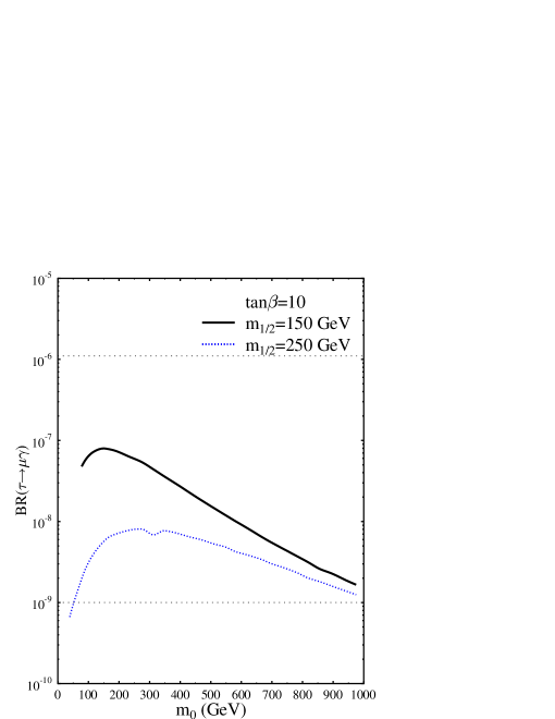
Figure 2: Branching ratio of $\tau\rightarrow\mu\gamma$ as a function of $m_{0}$ for $A_{0}=m_{0}$, $\tan\beta=10$ and $m_{\frac{1}{2}}=150GeV,\ 250GeV$. The dotted lines are the present upper bound and the expected sensitivity.

Br($\tau\to\mu\gamma$) is plotted in FIG. 2 for a typical set of SUSY parameters. We notice that in a quite large parameter space the process $\tau\to\mu\gamma$, induced in supersymmetric see-saw mechanism, is below the present experimental bound, $1.1\times 10^{-6}$pdg , while, will be detected in the future experiment if the expected sensitivity can reach down to $10^{-9}$ellis . In our calculation the SUSY parameters are constrained by the $g_{\mu}-2$ anomalyg-2 , so $m_{\frac{1}{2}}$ can not be too large.

The branching ratio of $\mu\to e\gamma$ is approximately proportional to $|{(V_{D})}_{13}{(V_{D})}_{23}|^{2}$. The element ${(V_{D})}_{13}$ seems quite model-dependent. However, under the following observations and assumptions, we find that a general prediction of ${(V_{D})}_{13}$ in this kind of models is possiblebi2 .

First, we assume that $Y_{N}$ has a similar hierarchical structure as the Yukawa coupling matrix of the up-type quark, $Y_{u}$. In SO(10) grand unified models, the simplest symmetry breaking mechanism leads to $Y_{N}=Y_{u}$. Since the see-saw mechanism is usually realized in an SO(10) grand unified model, this assumption is quite general. $Y_{u}$ is constrained by the values of up-type quark masses and the CKM mixing angles. By our second assumption that there is no accidental cancellation between the mixing matrices for the up- and down-type quarks leading to small CKM mixing, we then have

$$\theta_{u}^{13}\lesssim V_{td}\sim 0.008\ ,$$ (29)

with $\theta_{u}^{13}$ and $V_{td}$ being the 1-3 mixing angle produced by $Y_{u}$ and the 3-1 element of the CKM matrix. We thus expect that the 1-3 mixing angle produced by $Y_{N}$, ${\theta}_{N}^{13}$, is of the same order of magnitude as $\theta_{u}^{13}$. Then we have ${\theta}_{N}^{13}\lesssim 0.008$. Analogously, we have $\sin{\theta}_{N}^{23}\lesssim V_{ts}\cong 0.04$. Third, we observed that in most models $m_{\tau}$ and $m_{\mu}$ got their masses mainly from the 2-3 block of the lepton mass matrix. The elements in the first row and the first column of $M_{L}$ are constrained by $m_{e}$. By this structure, as given in Eq. (10), one finds thatbarr ; frit

$$\sin{\theta}_{12}\sim\sqrt{m_{e}/m_{\mu}}\cong 0.07\ ,$$ (30)

and

$$\sin{\theta}_{13}\approx m_{\mu}/m_{\tau}\sin{\theta}_{12}\ll\sin{\theta}_{12}\ ,$$ (31)

with ${\theta}$ being mixing angles in $U_{L}$. Finally, taking into account that ${\theta}_{23}\sim\mathcal{O}(1)$ in “lopsided” models we get

$$({V_{D}})_{13} \approx \sin{\theta}_{12}\sin{\theta}_{23}\approx 0.05\ \ ,$$ (32)

$$({V_{D}})_{23} \approx -\sin{\theta}_{23}\approx-0.71\ \ .$$ (33)

Thus the angles in $U_{L}$ alone can determine $({V_{D}})_{13}$ and $({V_{D}})_{23}$. This conclusion certainly depends on the assumed forms of $Y_{L}$ and $Y_{N}$; nonetheless, it is correct in most published “lopsided” modelsalbright ; lopsid , which can be explicitly checked. In fact our assumptions are implied in these models.

Actually the above assumptions can be relaxed. Since Eq. (32) is one term, the dominant one here, of the full expressions for $({V_{D}})_{13}$, unless there is strong cancellation among these terms, do we always have $({V_{D}})_{13}$ to be $\mathcal{O}(0.05)$ or larger.

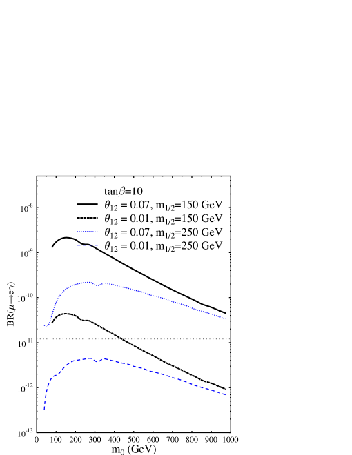
Figure 3: Br($\mu\to e\gamma$) as a function of $m_{0}$ for $\tan\beta=10$ and $m_{1/2}=150\,GeV,250\,GeV$. $A_{0}=m_{0}$ and $\mu>0$ are assumed. $\theta_{12}$ is the mixing angle between the $1^{st}$ & $2^{nd}$ generations in $U_{L}$. The horizontal dotted line is the present experimental limit, $1.2\times 10^{-11}$mueg .

In FIG. 3 we give our numerical result for Br($\mu\to e\gamma$). Taking $\tan\beta=10$ and $\theta_{12}=0.07$ as the typical value of the mixing angle between the $1^{st}$ and the $2^{nd}$ generations in $U_{L}$, we find that the predicted Br($\mu\to e\gamma$) has already exceeded the present upper bound, $1.2\times 10^{-11}$mueg . The other set of curves are for $\theta_{12}=0.01$ (corresponding to ${(V_{D})}_{13}=0.007$). In this case Br($\mu\to e\gamma$) may be below the experimental limit.

So large Br($\mu\to e\gamma$) is because of the large mixing angle $\theta_{23}$, which features the “lopsided” model and gives satisfied solution to large neutrino mixing. However, large $\theta_{23}$ enhances both ${(V_{D})}_{13}$ and ${(V_{D})}_{23}$, as given in Eqs. (32) and (33), leading to too large Br($\mu\to e\gamma$). This is really a dilemma. Another shortage of the “lopsided” model is that it generally predicts SMA or VAC solution to the solar neutrino problem, which are disfavored by present data. A recent work in Ref. albright predicts the LMA solution by “lopsided” structure. However, fine tuning to some extend is needed in this model. In next section we propose a new structure for $M_{L}$, which can solve the above problems simultaneously. The structure predicts very small ${(V_{D})}_{13}$ while, at the same time, LMA solution to the solar neutrinos.

V a new neutrino mass model

Assuming $Y_{N}$ is nearly diagonal we give

$$M_{L}=\left(\begin{array}[]{ccc}0&\delta&\sigma\\ -\delta&0&1-\epsilon\\ 0&\epsilon&1\end{array}\right)m,\ \ \text{with}\ \ \sigma\sim\mathcal{O}(1),\ \delta\ll\epsilon\ll 1\ .$$ (34)

Taking

$$\delta=0.00077,\ \epsilon=0.12,\ \text{and}\ \ \sigma=0.58$$ (35)

we can obtain the correct mass ratios $m_{e}/m_{\mu}$, $m_{\mu}/m_{\tau}$ and predict the neutrino mixing parameters as

$$\sin^{2}2\theta_{atm}=0.998,\tan^{2}\theta_{sol}=0.42\ \text{and}\ U_{e3}=-0.0054.$$ (36)

The notable feature of form (34) compared with the usual “lopsided” models is the $\mathcal{O}(1)$ element $\sigma$. Both the $(2,3)$ and $(1,3)$ elements in $M_{L}$ are large, naturally leading to large mixing angles, $\theta_{23}$ and $\theta_{12}$. The prediction of $U_{e3}=-0.0054$ is non-trivial, since the three parameters are fixed by the lepton mass ratios and one neutrino mixing angle. It thus provides a test of our model.

Diagonalizing $M_{L}$ analytically we can express $U_{e3}$ as

$$U_{e3}\cong\frac{m_{e}}{m_{\mu}}\cdot U_{\mu 3}/\tan\theta_{sol}\ .$$ (37)

This prediction that $U_{e3}$ is proportional to $m_{e}/m_{\mu}$ is unique. Usually $U_{e3}$ is predicted to be proportional to $\sqrt{m_{e}/m_{\mu}}$. Our model gives very small $U_{e3}$ value. Another interesting example which also gives quite small $U_{e3}$ is in Ref. xing , which predicts $U_{e3}=\sqrt{\frac{m_{e}}{m_{\tau}}}U_{\mu 3}$. However, this model predicts $\theta_{sol}\approx\pi/4$, which is excluded by present data.

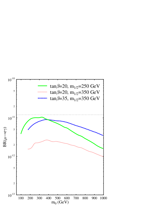
Figure 4: $Br(\mu\to e\gamma)$ predicted by our model as a function of $m_{0}$ for $\tan\beta=20$, $m_{1/2}=250\,GeV,350\,GeV$ and $\tan\beta=35$, $m_{1/2}=350\,GeV$. The horizontal dotted line is the present experimental limit, $1.2\times 10^{-11}$mueg .

The prediction of Br($\mu\to e\gamma$) by our model is plotted in FIG. 4. In most parameter space our model predicts Br($\mu\to e\gamma$) below the present experimental limit, while large enough to be detected in the next generation experimentnexp .

VI Summary and Conclusions

A quite popular theoretical scheme to explain the atmospheric and solar neutrino experiments is the see-saw mechanism together with the “lopsided” charged lepton mass matrix. This scheme is generally realized in the framework of supersymmetric grand unification. Our analysis shows that such a structure may predict big lepton flavor violation at low energy. The process $\tau\to\mu\gamma$ is quite promising to test whether there is a large mixing in the charged lepton sector, as predicted by “lopsided” models. In most SUSY parameter space this process will be detected in the next generation experiment. The “lopsided” models also make model-insensitive prediction about the process $\mu\rightarrow e\gamma$. However, the branching ratio of $\mu\rightarrow e\gamma$ predicted by these models generally exceeds the present experimental limit. An extended “lopsided” form of the charged lepton mass matrix is then proposed to solve this problem. The new structure can produce maximal 2-3 mixing, large 1-2 mixing while very small 1-3 mixing in the lepton sector. Br($\mu\rightarrow e\gamma$) is thus suppressed below the present experimental limit. The LMA solution for the solar neutrino problem is naturally produced.

- (1) Y. Fukuda et al., Super-Kamiokande Collaboration, Phys. Rev. Lett. 81 1562 (1998); 82 2644 (1999); 82 1810 (1999); 82 2430 (1999); Phys. Rev. Lett. 86 5651 (2001); M. B. Smy, Super-Kamiokande Collaboration, arXiv: hep-ex/0206016.
- (2) S. H. Ahn et al., K2K Collaboration, Phys. Lett. B511 178 (2001); Yuichi Oyama, K2K collaboration, arXiv: hep-ex/0210030; hep-ex/0104014; hep-ex/0004015.
- (3) Q. R. Ahmad et al., SNO Collaboration, Phys. Rev. Lett. 87, 071301 (2001); Phys. Rev. Lett. 89, 011301 (2002), arXiv: nucl-ex/0204008; Phys. Rev. Lett. 89, 011302 (2002), arXiv: nucl-ex/0204009.
- (4) T. Toshito, Super-Kamiokande Collaboration, arXiv: hep-ex/0105023; G. I. Fogli, E. Lisi and A. Marrone, arXiv: hep-ph/0110089; M. C. Gonzalez-Garcia and M. Maltoni, arXiv: hep-ph/0202218; M. Shiozawa, Super-Kamiokande Collaboration, Talk at Neutrino 2002, Munich May 2002.
- (5) Y. Fukuda et al., Super-Kamiokande Collaboration, Phys. Rev. Lett. 86 5656 (2001); The Super-Kamiokande Collaboration, Phys. Lett. B539 179 (2002), arXiv: hep-ex/0205075; M. B. Smy, Super-Kamiokande Collaboration, arXiv: hep-ex/0208004.
- (6) V. Barger, D. Marfatia, K. Whisnant and B. P. Wood, Phys. Lett. B 537, 179 (2002), arXiv:hep-ph/0204253; A. Bandyopadhyay, S. Choubey, S. Goswami and D. P. Roy, Phys. Lett. B 540, 14 (2002), arXiv:hep-ph/0204286; P. Creminelli, G. Signorelli and A. Strumia, arXiv:hep-ph/0102234 (version 3); P. Aliani, V. Antonelli, M. Picariello, R. Ferrari, E. Torrente-Lujan, arXiv:hep-ph/0205053; P. C. de Holanda and A. Y. Smirnov, arXiv:hep-ph/0205241; A. Strumia, C. Cattadori, N. Ferrari and F. Vissani, Phys. Lett. B 541, 327 (2002), arXiv:hep-ph/0205261; G. L. Fogli, E. Lisi, A. Marrone, D. Montanino and A. Palazzo, arXiv:hep-ph/0206162; M. Maltoni, T. Schwetz, M. A. Tortola and J. W. Valle, arXiv:hep-ph/0207227.
- (7) J. N. Bahcall, M. C. Gonzalez-Garcia and C. Pena-Garay, JHEP 0108, 014(2001); JHEP 0204 007 (2002), arXiv:hep-ph/0111150; JHEP 0207, 054 (2002), arXiv: hep-ph/0204314.
- (8) For a review, see: S. M. Barr and Ilja Dorsner, Nucl. Phys. B585, 79 (2000); Ilja Dorsner and S. M. Barr, Nucl. Phys. B617, 493 (2001) and references therein.
- (9) C. H. Albright and S.M. Barr, Phys. Rev. D 64, 073010 (2001); Phys. Rev. D 62, 093008 (2000); C. H. Albright, S. Geer, Phys. Rev. D 65, 073004 (2002); K. S. Babu, Jogesh C. Pati, Frank Wilczek, Nucl. Phys. B566, 33 (2000).
- (10) G. Altarelli, F. Feruglio and I. Masina, JHEP 0011, 040 (2000); K. Hagiwara and N. Okamura, Nucl. Phys. B548, 60 (1999); N. Irges, S. Lavignac and P. Ramond, Phys. Rev. D 58, 035003 (1998); M. Bando and T. Kugo, Prog. Theor. Phys. 101, 1313 (1999); M. Bando, T. Kugo, and K. Yoshioka, Prog. Theor. Phys. 104, 211 (2000); J. Sato and T. Yanagida, Phys. Lett. B430, 127 (1998); J. Sato and T. Yanagida, Phys. Lett. B493, 356 (2000); Z. Berezhiani and A. Rossi, JHEP 9903, 002 (1999); K.I. Izawa, K. Kurosawa, Y. Nomura, and T. Yanagida, Phys. Rev. D 60, 115016 (1999); R. Kitano and Y. Mimura, Phys. Rev. D 63, 016008 (2001); G. Altarelli and F. Feruglio, Phys. Lett. B451, 388 (1999); W. Buchmüller and T. Yanagida, Phys. Lett. B445, 399 (1998); Y. Nomura and T. Yanagida, Phys. Rev. D 59, 017303 (1999); N. Haba, Phys. Rev. D 59, 035011 (1999); P. Frampton and A. Rasin, Phys. Lett. B478, 424 (2000).
- (11) M. L. Brooks et al., MEGA Collaboration, Phys. Rev. Lett. 83, 1521 (1999).
- (12) H. P. Nills, Phys. Rep. 110, 1 (1984).
- (13) M. Dine and A. E. Nelson, Phys. Rev. D 48, 1277 (1993); G. F. Giudice and R. Rattazzi, Phys. Rep. 322, 419 (1999).
- (14) J. A. Casas, A. Ibarra, Nucl. Phys. B618, 171 (2001); J. Hisano and D. Nomura, Phys. Rev. D 59, 116005 (1999).
- (15) X. J. Bi, Y. B. Dai and X. Y. Qi, Phys. Rev. D63 096008 (2001).
- (16) K. Hagiwara et al., Phys. Rev. D 66, 01001 (2002).
- (17) John Ellis, M. E. Gomez, G. K. Leontaris, S. Lola and D. V. Nanopoulos, Eur. Phys. J. C14 (2000) 319.
- (18) G. W.Bennet et al., Muon g-2 Collaboration, Phys. Rev. Lett. 89, 101804 (2002); Erratum-ibid. 89, 129903 (2002), arXiv: hep-ex/0208001; H. N. Brown et al., Muon g-2 Collaboration Phys. Rev. Lett. 86, 2227 (2001).
- (19) X. J. Bi and Y. B. Dai, Phys. Rev. D66 076006 (2002).
- (20) H. Fritzsch and Z. Xing, Prog. Part. Nucl. Phys. 45, 1 (2000).
- (21) Z. Xing, Phys. Rev. D64, 093013 (2001).
- (22) L. M. Barkov et al., Research Proposal for an experiment at PSI (1999); M. Bachmann et al., MECO collaboration, Research Proposal E940 for an experiment at BNL (1997).