Axial charge segregation and $CP$ violation during the electroweak phase transition with hypermagnetic fields

Abstract

We study the scattering of fermions off the true vacuum bubbles nucleated during a first order electroweak phase transition in the presence of a background hypermagnetic field. By considering the limit of an infinitely thin bubble wall, we derive and analytically solve the Dirac equation in three spatial dimensions for left and right chirality modes and compute reflection and transmission coefficients for the case when the fermions move from the symmetric toward the broken symmetry phase. Given the chiral nature of the fermion coupling with the background field in the symmetric phase, an axial asymmetry is generated during the scattering processes. This mechanism is thus shown to provide an additional source of $CP$ violation within the standard model. We discuss possible implications for baryon number generation.

I Introduction

It is well known that the standard model (SM) of electroweak interactions meets all the requirements –known as Sakharov conditions Sakharov – to generate a baryon asymmetry during the electroweak phase transition (EWPT), provided that this last be of first order. As appealing as this scenario might be, it is also well known that neither the amount of $CP$ violation within the minimal SM nor the strength of the EWPT are enough to generate a sizable baryon number Gavela ; Kajantie .

Nonetheless, it has been recently shown that in the presence of large scale primordial magnetic fields it is possible to generate a stronger first order EWPT Giovannini ; Elmfors ; Giovannini2 . The situation is similar to what happens to a type I superconductor where an external magnetic field modifies the nature of the superconducting phase transition, changing it from second to first order due to the Meissner effect.

The presence of magnetic fields during the evolution of the early universe has neither been proved nor has it been ruled out. Temperature anisotropies measured by COBE place an upper bound $B_{0}\sim 10^{-9}\$G for homogeneous fields ($B_{0}$ refers to the intensity that the field would have today under the assumption of adiabatic decay due to the Hubble expansion) Barrow . In the case of inhomogeneous fields their effect must be searched for in the Doppler peaks Adams and in the polarization of the cosmic microwave background radiation Kosov . The future satellite missions MAP and PLANCK may reach the required sensitivity for the detection of these last signals.

Independently of their origin, there are several interesting cosmological consequences of the possible existence of primordial magnetic fields such as the generation of galactic seed fields and their influence on big bang nucleosynthesis reviews .

Recall that for temperatures above the EWPT, the SU(2)$\times$U(1)_Y symmetry is restored and the propagating, non-screened vector modes that represent a magnetic field correspond to the U(1)_Y group instead of to the U(1)_em group, and are therefore properly called hypermagnetic fields.

In previous works Ayala2 , it has been shown that another interesting cosmological consequence of the presence of such fields during the EWPT is the production of an axial charge segregation in the scattering of fermions off the true vacuum bubbles within the SM. This charge segregation is a consequence of the chiral nature of the fermion coupling to hypermagnetic fields in the symmetric phase. The analysis relied on the solution of an effectively one-dimensional Dirac equation for fermions moving perpendicular to the bubble wall.

In this paper, we lift this restriction and solve the Dirac equation in three spatial dimensions for the two chirality fermion modes in the presence of an external hypermagnetic field. Working in the limit of an infinitely thin bubble wall, we find analytical solutions –valid for fermion wave functions described by small quantum numbers– from where we compute reflection and transmission coefficients and show explicitly that these differ for left and right-handed chirality modes incident from the symmetric phase. Since these coefficients are related to the ones obtained by studying fermion incidence from the broken symmetry phase by $CPT$ and unitarity, we show how an axial charge segregation is built during the process. Such axial charge segregation provides a bias for baryon over antibaryon production and thus a seed for the non-local baryogenesis scenario Dine ; Cohen ; Nelson . We also discuss how this mechanism is equivalent to an extra source of $CP$ violation.

The outline of this work is as follows: In Sec. II, we write the Dirac equation for the left and right-handed chirality modes propagating in a background hypermagnetic field during the EWPT where the spatial profile of the Higgs field is taken in the limit of an infinitely thin wall. In Sec. III, we find the three dimensional solutions to this equation and discuss their properties. In Sec. IV, we use the solutions to compute reflection and transmission coefficients for axial fermion modes moving from the symmetric phase toward the broken symmetry phase. Finally in Sec. V, we conclude by looking out at the possible implications of such axially asymmetric fermion reflection and transmission.

II Dirac equation for chiral fermions in a background hypermagnetic field

During a first order EWPT, the properties of the nucleated bubbles depend on the effective, finite temperature Higgs potential. In the thin wall approximation and under the assumption that the phase transition happens when the energy densities of both phases are degenerate, it is possible to find a one-dimensional analytical solution for the Higgs field spatial profile $\phi(z)$ called the kink. This is given by

$$\phi(z)\sim 1+\tanh(z/\lambda)\,,$$ (1)

where $z$ is the coordinate along the direction of the phase change and $\lambda$ is the width of the wall.

When $\lambda$ is small compared to the mean free path, scattering within the wall is not affected by diffusion and the problem of fermion reflection and transmission through the wall can be cast in terms of solving the Dirac equation with a position dependent fermion mass, proportional to the Higgs field Ayala , where the proportionality constant is given by the particle’s Yukawa coupling. In physical terms, the wall can be considered thin when the spatial region where the fermion mass changes is small compared to other relevant length scales such as the particle mean free path.

In order to obtain analytical solutions, let us further simplify the problem considering the limit of an infinitely thin bubble wall, namely $\lambda\rightarrow 0$. In this case, the kink solution becomes a step function, $\Theta(z)$, and consequently, the expression for the particle’s mass becomes

$$m(z)=m_{0}\Theta(z)\,.$$ (2)

For $z\leq 0$ particles move in the region outside the bubble, that is, in the symmetric phase where particles are massless. Conversely, for $z\geq 0$, particles move inside the bubble, which represents the broken phase where particles have acquired a finite mass $m_{0}$.

In the presence of an external magnetic field, we need to consider that fermion modes couple differently to the field in the broken and the symmetric phases.

For $z\leq 0$, the coupling is chiral. Let

$$\Psi_{R} = \frac{1}{2}\left(1+\gamma_{5}\right)\Psi$$

$$\Psi_{L} = \frac{1}{2}\left(1-\gamma_{5}\right)\Psi$$ (3)

represent, as usual, the right and left-handed chirality modes for the spinor $\Psi$, respectively. Then, the equations of motion for these modes, as derived from the electroweak interaction Lagrangian, are

$$(i\partial\!\!\!\!\!\not\,\,\,\ -\ \frac{y_{L}}{2}g^{\prime}A\!\!\!\!\!\not\,\,\,\ )\Psi_{L}-m(z)\Psi_{R} = 0$$

$$(i\partial\!\!\!\!\!\not\,\,\,\ -\ \frac{y_{R}}{2}g^{\prime}A\!\!\!\!\!\not\,\,\,\ )\Psi_{R}-m(z)\Psi_{L} = 0\,,$$ (4)

where $y_{R,L}$ are the right and left-handed hypercharges corresponding to the given fermion, respectively, $g^{\prime}$ the $U(1)_{Y}$ coupling constant and we take $A^{\mu}=(0,{\mathbf{A}})$ representing a, not yet specified, four-vector potential having non-zero components only for its transverse spatial part, in the rest frame of the wall. This last requirement means that the corresponding magnetic field will point along the direction perpendicular to the wall.

The gauge field profile should correspond to our choice of Higgs field profile and thus the change in the magnetic field strength should take place in the same small spatial region over which the change in the Higgs field takes place. An exact treatment that considered a continuous change in the Higgs field would require that the gauge field be also continuous across the interface. Nonetheless, since we are pursuing insight from analytical results, we consider the simplified situation in which the gauge field is constant on either side of the wall and discontinuous at the planar phase boundary. A discussion on the consequences of considering a continuous gauge field profile can be found in the second of Refs. Ayala2 .

The set of Eqs. (4) can be written as a single equation for the spinor $\Psi=\Psi_{R}+\Psi_{L}$ by adding them up

$$\left\{i\partial\!\!\!\!\!\not\,\,\,\ -A\!\!\!\!\!\not\,\,\,\left[\frac{y_{R}}{4}g^{\prime}\left(1+\gamma_{5}\right)+\frac{y_{L}}{4}g^{\prime}\left(1-\gamma_{5}\right)\right]-m(z)\right\}\Psi=0\,.$$ (5)

Hereafter, we explicitly work in the chiral representation of the gamma matrices where

$$\gamma^{0}=\!\left(\begin{array}[]{rr}0&-I\\ -I&0\end{array}\right)\ \mbox{\boldmath$\gamma$}=\!\left(\begin{array}[]{rr}0&\mbox{\boldmath$\sigma$}\\ \mbox{\boldmath$-\sigma$}&0\end{array}\right)\ \gamma_{5}=\!\left(\begin{array}[]{rr}I&0\\ 0&-I\end{array}\right)\,.$$ (12)

Within this representation, we can write Eq. (5) as

$$\Big{\{}i\partial\!\!\!\!\!\not\,\,\,\ -\ {\mathcal{G}}A_{\mu}\gamma^{\mu}-m(z)\Big{\}}\Psi=0\,,$$ (13)

where we have introduced the matrix

$${\mathcal{G}}=\left(\begin{array}[]{cc}\frac{y_{L}}{2}g^{\prime}I&0\\ 0&\frac{y_{R}}{2}g^{\prime}I\end{array}\right)\,.$$ (16)

We now look at the corresponding equation in the broken symmetry phase. For $z\geq 0$ the coupling of the fermion with the external field is through the electric charge $e$ and thus, the equation of motion is simply the Dirac equation describing an electrically charged fermion in a background magnetic field, namely,

$$\Big{\{}i\partial\!\!\!\!\!\not\,\,\,\ -\ eA_{\mu}\gamma^{\mu}-m(z)\Big{\}}\Psi=0\,.$$ (17)

In the following section, we explicitly construct the solutions to Eqs. (13) and  (17) with a constant magnetic field, requiring that these match at the interface $z=0$.

III Solving the Dirac Equation

For definiteness, let us consider a constant magnetic field ${\mathbf{B}}=B\hat{z}$ pointing along the $\hat{z}$ direction. We first look for the stationary solutions of Eq. (13) corresponding to fermions moving in the symmetric phase. Writing

$$\Psi({\bf r},t)=e^{-iEt}\Psi({\bf r})\,,$$ (18)

where

$$\Psi({\bf r})=\left(\begin{array}[]{c}\psi_{1}({\bf r})\\ \psi_{2}({\bf r})\\ \psi_{3}({\bf r})\\ \psi_{4}({\bf r})\end{array}\right)\,,$$ (23)

and working in the chiral representation of the gamma matrices, Eq. (13) becomes explicitly

$$E\psi_{1}({\bf r})-(P_{x}^{R}-iP_{y}^{R})\psi_{2}({\bf r})-P_{z}\psi_{1}({\bf r}) = 0$$

$$E\psi_{2}({\bf r})-(P_{x}^{R}+iP_{y}^{R})\psi_{1}({\bf r})+P_{z}\psi_{2}({\bf r}) = 0$$

$$E\psi_{3}({\bf r})+(P_{x}^{L}-iP_{y}^{L})\psi_{4}({\bf r})+P_{z}\psi_{3}({\bf r}) = 0$$

$$E\psi_{4}({\bf r})+(P_{x}^{L}+iP_{y}^{L})\psi_{3}({\bf r})-P_{z}\psi_{4}({\bf r}) = 0\,,$$ (24)

where we introduced the definitions

$${\mathbf{P}}^{R} \equiv -i\nabla+\frac{y^{R}g^{\prime}}{2}{\mathbf{A}}$$

$${\mathbf{P}}^{L} \equiv -i\nabla+\frac{y^{L}g^{\prime}}{2}{\mathbf{A}}\,.$$ (25)

Since $A_{z}=0$,

$$P_{z}^{R}=P_{z}^{L}\equiv P_{z}\,.$$ (26)

In this representation $\psi_{1,2}$ and $\psi_{3,4}$ correspond to components with right- and left-handed chirality, respectively. Notice that, since in the symmetric phase fermions are massless, the differential Eqs. (24) do not mix components with different chirality.

Let us now work in cylindrical coordinates and look for solutions of the form

$$\Psi(r,\phi,z)\sim\left(\begin{array}[]{c}f_{1}(r)e^{-i\phi/2}\\ f_{2}(r)e^{+i\phi/2}\\ f_{3}(r)e^{-i\phi/2}\\ f_{4}(r)e^{+i\phi/2}\\ \end{array}\right)e^{i(l-\frac{1}{2})\phi}e^{ikz}\,.$$ (31)

Using the explicit components of the vector ${\bf A}({\bf r})$ that produce a constant magnetic field along the $\hat{z}$ axis, it is easy to show that Sokolov

$$P_{x}^{R,L}\pm iP_{y}^{R,L}=-ie^{\pm i\phi}\left(\frac{\partial}{\partial r}\pm\frac{i}{r}\frac{\partial}{\partial\phi}\mp\gamma^{R,L}r\right)\,,$$ (32)

which, together with the definitions

$$\gamma^{R,L} \equiv \frac{y^{R,L}g^{\prime}}{4}B$$

$$\rho^{R,L} \equiv \gamma^{R,L}r^{2}$$

$${\cal R}^{R,L}_{1} \equiv (\gamma^{R,L}\rho^{R,L})^{1/2}\left(2\frac{d}{d\rho^{R,L}}-1-\frac{(l-1)}{\rho^{R,L}}\right)$$

$${\cal R}^{R,L}_{2} \equiv (\gamma^{R,L}\rho^{R,L})^{1/2}\left(2\frac{d}{d\rho^{R,L}}+1+\frac{l}{\rho^{R,L}}\right)\,,$$ (33)

make the set of Eqs.(24) to be explicitly written as

$$(E-k)f_{1}(\rho^{R})+i{\cal R}^{R}_{2}f_{2}(\rho^{R}) = 0$$

$$(E+k)f_{2}(\rho^{R})+i{\cal R}^{R}_{1}f_{1}(\rho^{R}) = 0$$

$$(E+k)f_{3}(\rho^{L})+i{\cal R}^{L}_{2}f_{4}(\rho^{L}) = 0$$

$$(E-k)f_{4}(\rho^{L})+i{\cal R}^{L}_{1}f_{3}(\rho^{L}) = 0\,.$$ (34)

By acting on Eqs. (34) with $i{\cal R}^{R}_{1}$, $i{\cal R}^{R}_{2}$, $i{\cal R}^{L}_{1}$ and $i{\cal R}^{L}_{2}$, respectively, we obtain the set of second order differential equations

$$\left\{\rho^{R}\frac{d^{2}}{d(\rho^{R})^{2}}+\frac{d}{d\rho^{R}}+\lambda^{R}-\frac{l}{2}-\frac{\rho^{R}}{4}-\frac{(l-1)^{2}}{4\rho^{R}}\right\}f_{1}(\rho^{R}) = 0$$

$$\left\{\rho^{R}\frac{d^{2}}{d(\rho^{R})^{2}}+\frac{d}{d\rho^{R}}+\lambda^{R}-\frac{(l-1)}{2}-\frac{\rho^{R}}{4}-\frac{l^{2}}{4\rho^{R}}\right\}f_{2}(\rho^{R}) = 0$$

$$\left\{\rho^{L}\frac{d^{2}}{d(\rho^{L})^{2}}+\frac{d}{d\rho^{L}}+\lambda^{L}-\frac{l}{2}-\frac{\rho^{L}}{4}-\frac{(l-1)^{2}}{4\rho^{L}}\right\}f_{3}(\rho^{L}) = 0$$

$$\left\{\rho^{L}\frac{d^{2}}{d(\rho^{L})^{2}}+\frac{d}{d\rho^{L}}+\lambda^{L}-\frac{(l-1)}{2}-\frac{\rho^{L}}{4}-\frac{l^{2}}{4\rho^{L}}\right\}f_{4}(\rho^{L}) = 0\,,$$ (35)

where

$$\lambda^{R,L}\equiv\frac{E^{2}-(k^{R,L})^{2}}{4\gamma^{R,L}}\,.$$ (36)

The eigenvalues $\lambda^{R,L}$ corresponding to the requirement that the solutions vanish as $\rho^{R,L}\rightarrow\infty$ are such that

$$\lambda^{R,L}=n\,.$$ (37)

$n=l+s$ is called the principal quantum number which must be a non-negative integer $n=0,1,2,3\ldots$ From Eq. (36), the spectrum is given by

$$E=\sqrt{(k^{R,L})^{2}+4n\gamma^{R,L}}\,.$$ (38)

The solutions to Eqs. (35) are

$$f_{1}(\rho^{R}) = C_{1}I_{n-1,s}(\rho^{R})$$

$$f_{2}(\rho^{R}) = iC_{2}I_{n,s}(\rho^{R})$$

$$f_{3}(\rho^{L}) = C_{3}I_{n-1,s}(\rho^{L})$$

$$f_{4}(\rho^{L}) = iC_{4}I_{n,s}(\rho^{L})\,,$$ (39)

where $C_{1,\ldots,4}$ are constants and $I_{n,s}(\rho)$ are the Laguerre functions given in terms of the Laguerre polynomials $Q_{s}^{n-s}$ by

$$I_{n,s}(\rho)=\frac{1}{(n!s!)^{1/2}}e^{-\rho/2}\rho^{(n-s)/2}Q_{s}^{n-s}(\rho)\,,$$ (40)

satisfying the normalization condition

$$\int_{0}^{\infty}d\rho I_{n,s}^{2}(\rho)=1\,.$$ (41)

Using the recurrence relations for the Laguerre polynomials together with the set of Eqs. (24), one readily obtains that the constants $C_{1,2}$ and $C_{3,4}$ are not independent and thus that the solution $\Psi({\bf r})$ for fermions moving in the symmetric phase is given by

$$\Psi(r,\phi,z)=\left(\begin{array}[]{c}C_{2}\left\{\begin{array}[]{c}\sqrt{\frac{E+k^{R}}{E-k^{R}}}I_{n-1,s}(\rho^{R})e^{i(l-1)\phi}\\ iI_{n,s}(\rho^{R})e^{il\phi}\end{array}\right\}e^{ik^{R}z}\\ C_{3}\left\{\begin{array}[]{c}I_{n-1,s}(\rho^{L})e^{i(l-1)\phi}\\ i\sqrt{\frac{E+k^{L}}{E-k^{L}}}I_{n,s}(\rho^{L})e^{il\phi}\end{array}\right\}e^{ik^{L}z}\end{array}\right)\,.$$ (48)

We now turn to finding the solutions to Eq. (17), namely, for fermions moving in the broken symmetry phase. By a procedure similar to the above, it is easy to see that the solutions are given by Sokolov

$$\Psi(r,\phi,z)=\left(\begin{array}[]{l}D_{1}I_{n^{\prime}-1,s^{\prime}}(\rho)e^{i(l^{\prime}-1)\phi}\\ iD_{2}I_{n^{\prime},s^{\prime}}(\rho)e^{il^{\prime}\phi}\\ D_{3}I_{n^{\prime}-1,s^{\prime}}(\rho)e^{i(l^{\prime}-1)\phi}\\ iD_{4}I_{n^{\prime},s^{\prime}}(\rho)e^{il^{\prime}\phi}\end{array}\right)e^{ikz}\,,$$ (53)

where

$$\rho \equiv \gamma r^{2}$$

$$\gamma \equiv \frac{g^{\prime}}{2}B\,.$$ (54)

Notice that in the second of Eqs. (54), we have used that since in the broken symmetry phase there should not be a propagating component corresponding to the $Z^{0}$ field Giovannini ; Elmfors , the parameter representing the magnetic field strength $B^{\prime}$ is related to $B$ and Weinberg’s angle $\theta_{W}$ by

$$B^{\prime}=\frac{B}{\cos\theta_{W}}\,,$$ (55)

which in turn implies that the coupling of the fermion with the magnetic field in the broken symmetry phase $eB^{\prime}$ becomes

$$eB^{\prime}=g^{\prime}B\,.$$ (56)

The spectrum is given by $E=\sqrt{k^{2}+m_{0}^{2}+4n^{\prime}\gamma}$, with $n^{\prime}=l^{\prime}+s^{\prime}$ being a non-negative integer $n^{\prime}=0,1,2\ldots$. The constants $D_{1,\ldots,4}$ are not independent from each other and are given in terms of the two constants $G_{1}$ and $G_{2}$ by

$$\left(\begin{array}[]{c}D_{1}\\ D_{2}\\ D_{3}\\ D_{4}\end{array}\right)=G_{1}\left(\begin{array}[]{c}-\frac{\sqrt{E^{2}-k^{2}-m_{0}^{2}}}{m_{0}}\\ -\frac{(E-k)}{m_{0}}\\ 0\\ 1\end{array}\right)+G_{2}\left(\begin{array}[]{c}-\frac{(E+k)}{m_{0}}\\ -\frac{\sqrt{E^{2}-k^{2}-m_{0}^{2}}}{m_{0}}\\ 1\\ 0\end{array}\right)\,.$$ (69)

In order to describe the motion of fermions in the whole domain, we should now proceed to join the solutions in Eqs. (48) and (53) across the interface at $z=0$. To this end, we work in the approximation where the incident fermions from the symmetric phase make energy and angular momentum conserving transitions to states with the same principal quantum number in the broken symmetry phase, namely $n=n^{\prime}$ and $l=l^{\prime}$, which requires $s=s^{\prime}$. This approximation corresponds to the classical picture in which the effect of a sudden change in the coupling with the external field produces only a change in the radius of the orbit around the field lines. This is a reasonable approximation as long as the number of quanta in the transverse modes for a given energy is not too large. This can be quantified by considering the overlap of the radial functions $I_{n,s}(\rho^{R,L})$ and $I_{n^{\prime},s^{\prime}}(\rho)$ for $l=l^{\prime}$ as a function of $s^{\prime}-s$, as shown in Fig. 1. We find that our approximation is valid for low values of $s$ and $l$. Otherwise, interference with modes with additional nodes associated with large values of these quantum numbers is not negligible, which means these modes need to be considered in the complete solution.

For fermions incident from the symmetric phase, the complete wave function contains incoming as well as outgoing components, whereas in the broken symmetry phase the wave function corresponds to only outgoing waves. To describe the scattering of right- and left-handed chirality modes, let us consider them separately.

For right-handed incident modes, continuity of the solution across the interface yields the system of conditions

$$\sqrt{\frac{E+k^{R}}{E-k^{R}}}+\left(\sqrt{\frac{E-k^{R}}{E+k^{R}}}\ \right)C_{2}^{R} = -\left(\frac{\sqrt{E^{2}-k^{2}-m_{0}^{2}}}{m_{0}}\ \right)G_{1}^{R}-\left(\frac{E+k}{m_{0}}\right)G_{2}^{R}$$

$$1+C_{2}^{R} = -\left(\frac{E-k}{m_{0}}\right)G_{1}^{R}-\left(\frac{\sqrt{E^{2}-k^{2}-m_{0}^{2}}}{m_{0}}\ \right)G_{2}^{R}$$

$$C_{3}^{R} = G_{2}^{R}$$

$$\left(\sqrt{\frac{E-k^{L}}{E+k^{L}}}\ \right)C_{3}^{R} = G_{1}^{R}\,.$$ (70)

On the other hand, for left-handed incident modes, continuity of the solution across the interface yields the system of conditions

$$\left(\sqrt{\frac{E-k^{R}}{E+k^{R}}}\ \right)C_{2}^{L} = -\left(\frac{\sqrt{E^{2}-k^{2}-m_{0}^{2}}}{m_{0}}\ \right)G_{1}^{L}-\left(\frac{E+k}{m_{0}}\right)G_{2}^{L}$$

$$C_{2}^{L} = -\left(\frac{E-k}{m_{0}}\right)G_{1}^{L}-\left(\frac{\sqrt{E^{2}-k^{2}-m_{0}^{2}}}{m_{0}}\ \right)G_{2}^{L}$$

$$1+C_{3}^{L} = G_{2}^{L}$$

$$\left(\sqrt{\frac{E+k^{L}}{E-k^{L}}}\ \right)+\left(\sqrt{\frac{E-k^{L}}{E+k^{L}}}\ \right)C_{3}^{L} = G_{1}^{L}\,.$$ (71)

Eqs. (70) and (71) completely determine the constants $C_{2,3}^{R}$, $G_{1,2}^{R}$ and $C_{2,3}^{L}$, $G_{1,2}^{L}$, respectively.

IV Transmission and reflection coefficients

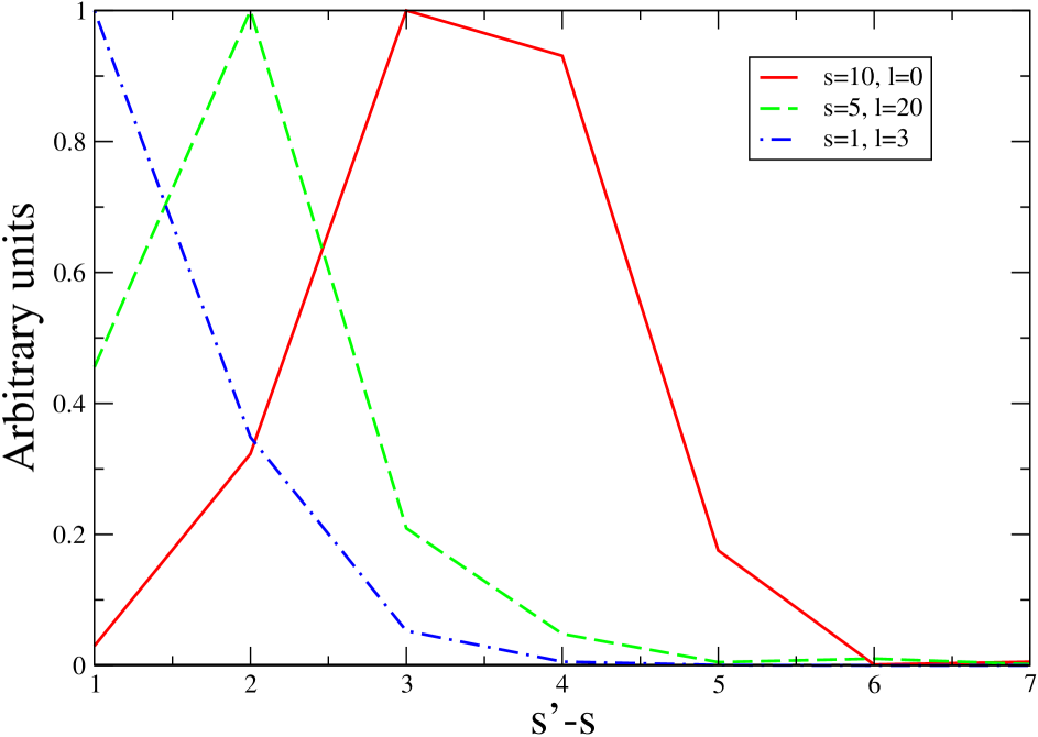
Figure 1: Overlap integral for the functions $I_{n,s}(\rho^{R})$ and $I_{n^{\prime},s^{\prime}}(\rho)$ normalized to the maximum value in each case for $l=l^{\prime}$ as a function of $s^{\prime}-s$ for three different values of the pairs $s$ and $l$. Notice that when $s$ and $l$ are large, the overlap is maximum for $s^{\prime}\neq s$.

The fact that the solutions to the systems of Eqs. (70) and (71) are not the same, means that there is the possibility of building an axial asymmetry during the scattering of fermions off the wall. To quantify the asymmetry, we need to compute the corresponding reflection and transmission coefficients. These are built from the reflected, transmitted and incident currents of each type. Recall that for a given spinor wave function $\Psi$, the current normal to the wall is given by

$$J=\int_{0}^{\infty}d\rho\int_{0}^{2\pi}d\phi\Psi^{\dagger}(\rho,\phi,z)\gamma^{0}\gamma^{3}\Psi(\rho,\phi,z)\,.$$ (72)

For right-handed incoming waves, the incident current $J^{R}_{\mbox{\small inc}}$ is thus given by

$$J^{R}_{\mbox{\small inc}}=\frac{2k^{R}}{E-k^{R}}$$ (73)

whereas the reflected and transmitted currents $J^{R}_{\mbox{\small ref}}$, $J^{R}_{\mbox{\small tra}}$ are given respectively by

$$J^{R}_{\mbox{\small ref}} = \left(\frac{2k^{R}}{E+k^{R}}\right)(C_{2}^{R})^{2}+\left(\frac{2k^{L}}{E+k^{L}}\right)(C_{3}^{R})^{2}$$

$$J^{R}_{\mbox{\small tra}} = \left[\left(\frac{\sqrt{E^{2}-k^{2}-m_{0}^{2}}}{m_{0}}\ \right)G_{1}^{R}+\left(\frac{E+k}{m_{0}}\right)G_{2}^{R}\right]^{2}$$ (74)

$$- \left[\left(\frac{\sqrt{E^{2}-k^{2}-m_{0}^{2}}}{m_{0}}\ \right)G_{2}^{R}+\left(\frac{E-k}{m_{0}}\right)G_{1}^{R}\right]^{2}$$

$$- (G_{2}^{R})^{2}+(G_{1}^{R})^{2}\,.$$

On the other hand, for left-handed incoming waves, the incident current $J^{L}_{\mbox{\small inc}}$ is given by

$$J^{L}_{\mbox{\small inc}}=\frac{2k^{L}}{E-k^{L}}$$ (75)

and the reflected and transmitted currents $J^{L}_{\mbox{\small ref}}$, $J^{L}_{\mbox{\small tra}}$ are given respectively by

$$J^{L}_{\mbox{\small ref}} = \left(\frac{2k^{R}}{E+k^{R}}\right)(C_{2}^{L})^{2}+\left(\frac{2k^{L}}{E+k^{L}}\right)(C_{3}^{L})^{2}$$

$$J^{L}_{\mbox{\small tra}} = \left[\left(\frac{\sqrt{E^{2}-k^{2}-m_{0}^{2}}}{m_{0}}\ \right)G_{1}^{L}+\left(\frac{E+k}{m_{0}}\right)G_{2}^{L}\right]^{2}$$ (76)

$$- \left[\left(\frac{\sqrt{E^{2}-k^{2}-m_{0}^{2}}}{m_{0}}\ \right)G_{2}^{L}+\left(\frac{E-k}{m_{0}}\right)G_{1}^{L}\right]^{2}$$

$$- (G_{2}^{L})^{2}+(G_{1}^{L})^{2}\,.$$

Recall that in the symmetric phase, where fermions are massless, the chirality and helicity operators commute and thus chirality modes are also eigenfunctions of helicity. From Eq. (48) and the representation of the gamma matrices, Eq. (12), we see that for right-(left) handed chirality modes, the large components correspond to right-(left) handed helicity modes. Since scattering of the wall does not change the spin direction of the impinging particle, right-(left) handed helicity modes reflect as left-(right) handed and transmit as right-(left) handed modes. To emphasize this point, for the reflection and transmission coefficients, let us denote by lower case letters $r$ and $l$ the right- and left-handed helicity modes. These coefficients are given as the ratios of the corresponding reflected and transmitted currents, to the incident one, explicitly

$$R_{r\rightarrow l} = J_{\mbox{\small ref}}^{R}/J_{\mbox{\small inc}}^{R}$$

$$T_{r\rightarrow r} = J_{\mbox{\small tra}}^{R}/J_{\mbox{\small inc}}^{R}\,.$$ (77)

The corresponding coefficients for the axially conjugate process are

$$R_{l\rightarrow r} = J_{\mbox{\small ref}}^{L}/J_{\mbox{\small inc}}^{L}$$

$$T_{l\rightarrow l} = J_{\mbox{\small tra}}^{L}/J_{\mbox{\small inc}}^{L}\,.$$ (78)

Using Eqs. (73) to (74), together with the solutions to Eqs. (70) and (71), it is straightforward to show that

$$R_{r\rightarrow l}+T_{r\rightarrow r} = 1$$

$$R_{l\rightarrow r}+T_{l\rightarrow l} = 1$$ (79)

Figure 2 shows the coefficients $R_{l\rightarrow r}$ and $R_{r\rightarrow l}$ as a function of the magnetic field $B$ scaled by $m_{0}^{2}$ for $E/m_{0}=3$, $n=1$ and hypercharge values for top quarks $y_{R}=4/3$, $y_{L}=1/3$, with $g^{\prime}=0.344$, as appropriate for the EWPT epoch. Notice that when $b\rightarrow 0$, these coefficients approach each other and that the difference grows with increasing field strength.

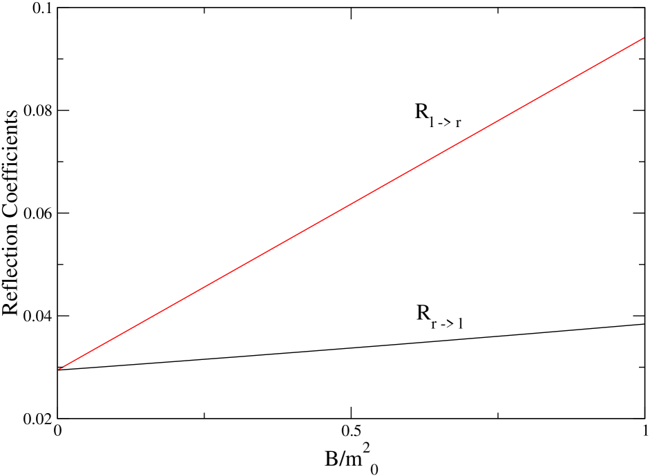
Figure 2: Coefficients $R_{l\rightarrow r}$ and $R_{r\rightarrow l}$ as a function of the magnetic field $B$ scaled by $m_{0}^{2}$ for $E/m_{0}=3$, $n=1$, and $y_{R}=4/3$, $y_{L}=1/3$. The value for the $U(1)_{Y}$ coupling constant is taken as $g^{\prime}=0.344$, corresponding to the EWPT epoch.

Figure 3 shows the reflection and transmission coefficients as a function of energy scaled by the fermion mass $m_{0}$. Figure 3a shows the coefficients $R_{r\rightarrow l}$ and $T_{r\rightarrow r}$ and Fig. 3b the coefficients $R_{l\rightarrow r}$ and $T_{l\rightarrow l}$ for $B/m_{0}^{2}=0.5$ and $n=1$, $y_{R}=4/3$, $y_{L}=1/3$, $g^{\prime}=0.344$. Since the solutions in Eqs. (53) are computed assuming that the transmitted waves are not exponentially damped, their energies have to be taken such that $E\geq\sqrt{m_{0}^{2}+4n\gamma}$. For these energy values, there is thus no need to consider the contribution from negative-energy solutions Bjorken .

V Discussion and Conclusions

In this paper we have derived and solved the Dirac equation describing fermions scattering off a first order EWPT bubble wall in three spatial dimensions, in the approximation of an infinitely thin wall, in the presence of a magnetic field directed along the fermion direction of motion. In the symmetric phase, the fermions couple chirally to the magnetic field, which receives the name of hypermagnetic, given that it belongs to the $U(1)_{Y}$ group. We have shown that the chiral nature of this coupling implies that it is possible to build an axial asymmetry during the scattering of fermions off the wall. We have computed reflection and transmission coefficients showing explicitly that they differ for left and right-handed incident particles from the symmetric phase. The results of this calculation are in agreement with those previously found in Refs. Ayala2 , where the motion of the fermions was effectively treated as one-dimensional.

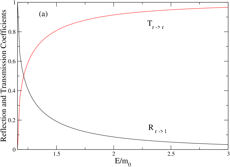
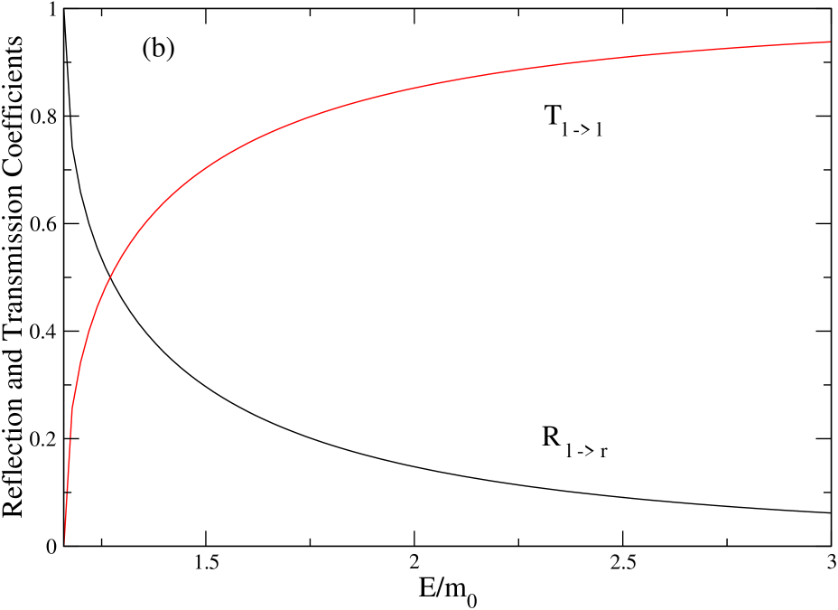
Figure 3: Reflection and transmission coefficients as a function of energy scaled by the fermion mass for $B/m_{0}^{2}=0.5$, $n=1$, $y_{R}=4/3$, $y_{L}=1/3$, $g^{\prime}=0.344$. (a) Shows the coefficients for incident, right-handed helicity modes and (b) for incident, left-handed helicity modes.

The three dimensional treatment of the problem allows for a clearer physical picture of the fermion motion in the presence of the external field: Suppose that the original fermion motion is not parallel to the direction of the field lines and therefore that its velocity vector contains a component perpendicular to the field. In this case, due to the Lorentz force, the particle circles around the field lines maintaining its velocity along the direction of the field. The motion of the particle is thus described as an overall displacement along the field lines superimposed to a circular motion around these lines. These circles correspond to the different quantum levels, labeled by $n$, the principal quantum number. We see that the originally different angles of incidence all result in the same overall direction of incidence. Also, since the relevant quantities that determine the strength of the coupling are the magnitudes of the parameters $\gamma^{R,L}$ and $\gamma$, the generated axial asymmetry is independent of whether the fermion moves parallel or anti-parallel to the field lines.

What is the relation of this axial asymmetry to $CP$ violation? Recall that in the SM, $CP$ is violated in the quark sector through the mixing between different weak interaction eigenstates to form states with definite mass. However, in the present scenario, taking place within the SM, no such mixing occurs since we are concerned only with the evolution of a single quark (for instance, the top quark) species. The relation is thus to be found in the dynamics of the scattering process itself and becomes clear once we notice that this can be thought of as describing the mixing of two levels, right- and left-handed quarks coupled to an external hypermagnetic field. When the two chirality modes interact only with the external field, they evolve separately, as described by Eq. (48). It is only the scattering with the bubble wall what allows a finite transition probability for one mode to become the other. Since the modes are coupled differently to the external field, these probabilities are different and give rise to the axial asymmetry. $CP$ is violated in the process because, though $C$ is conserved, $P$ is violated and thus is $CP$.

We also emphasize that, under the very general assumptions of $CPT$ invariance and unitarity, the total axial asymmetry (which includes contributions both from particles and antiparticles) is quantified in terms of the particle (axial) asymmetry. Let $\rho_{i}$ represent the number density for species $i$. The net densities in left-handed and right-handed axial charges are obtained by taking the differences $\rho_{L}-\rho_{\bar{L}}$ and $\rho_{R}-\rho_{\bar{R}}$, respectively. It is straightforward to show Nelson that $CPT$ invariance and unitarity imply that the above net densities are given by

$$\rho_{L}-\rho_{\bar{L}} = (f^{s}-f^{b})(R_{r\rightarrow l}-R_{l\rightarrow r})$$

$$\rho_{R}-\rho_{\bar{R}} = (f^{s}-f^{b})(R_{l\rightarrow r}-R_{r\rightarrow l})\,,$$ (80)

where $f^{s}$ and $f^{b}$ are the statistical distributions for particles or antiparticles (since the chemical potentials are assumed to be zero or small compared to the temperature, these distributions are the same for particles or antiparticles) in the symmetric and the broken symmetry phases, respectively. From Eq. (80), the asymmetry in the axial charge density is finally given by

$$(\rho_{L}-\rho_{\bar{L}})-(\rho_{R}-\rho_{\bar{R}})=2(f^{s}-f^{b})(R_{r\rightarrow l}-R_{l\rightarrow r}).$$ (81)

This asymmetry, built on either side of the wall, is dissociated from non-conserving baryon number processes and can subsequently be converted to baryon number in the broken symmetry phase where sphaleron induced transitions are taking place with a large rate. This mechanism receives the name of non-local baryogenesis Dine ; Nelson ; Cohen ; Joyce and, in the absence of the external field, it can only be realized in extensions of the SM where a source of $CP$ violation is introduced ad hoc into a complex, space-dependent phase of the Higgs field during the development of the EWPT Torrente .

An interesting possibility to extend the scope of the present work is to study the scattering of fermions in the presence of topologically non-trivial configurations of hypermagnetic fields such as the so called, hypermagnetic knots which themselves can seed the baryon asymmetry of the universe in extensions of the SM Giovannini2 .

Since another consequence of the existence of an external magnetic field is the lowering of the barrier between topologically inequivalent vacua Comelli , due to the sphaleron dipole moment, the use of the mechanism discussed in this work to possibly generate a baryon asymmetry is not as straightforward. Nonetheless, if such primordial fields indeed existed during the EWPT epoch and the phase transition was first order, as is the case, for instance, in minimal extensions of the SM, the mechanism advocated in this work has to be considered as acting in the same manner as a source of $CP$ violation that can have important consequences for the generation of a baryon number.

References

• (1) A. D. Sakharov, Pisโ€™ma Zh. Eksp. Teor. Fiz. 5, 32 (1967) [JETP Lett. 5, 24 (1967)].
• (2) M.B. Gavela, P. Hernรกndez, J. Orloff, and O. Pรจne, Mod. Phys. Lett. A9, 795 (1994).
• (3) K. Kajantie, M. Laine, K. Rummukainen, and M. Shaposnikov, Nucl. Phys. B 466, 189 (1996).
• (4) M. Giovannini and M. E. Shaposhnikov, Phys.ย Rev.ย D57, 2186 (1998).
• (5) P. Elmfors, K. Enqvist and K. Kainulainen, Phys. Lett. B 440, 269 (1998).
• (6) M. Giovannini, Phys.ย Rev.ย D61, 063004 (2000); Phys.ย Rev.ย D61, 063502 (2000).
• (7) J.D. Barrow, P.G. Ferreira and J. Silk, Phys. Rev. Lett. 78, 3610 (1997).
• (8) J. Adams, U.H. Danielsson, D. Grasso and H. Rubinstein, Phys.ย Lett.ย B 388, 253 (1996).
• (9) A. Kosovsky and A. Loeb, Ap. J. 469, 1 (1996); E. S. Scannapieco and P.G. Ferreira, Phys. Rev. D 56, 7493 (1997); R. Durrer, P. G. Ferreira and T. Kahniashvili, Phys.ย Rev.ย D61, 043001 (2000); K. Jedamzik, V. Kataliniฤ‡ and A. V. Olinto, Phys.ย Rev.ย Lett.ย 85, 700 (2000).
• (10) For recent reviews on the origin, evolution and some cosmological consequences of primordial magnetic fields see: K. Enqvist, Int. J. Mod. Phys. D7, 331 (1998); R. Maartens, International Conference on Gravitation and Cosmology, India, Jan. 2000, [Pramana 55, 575 (2000)] and references therein; D. Grasso and H.R. Rubinstein, Phys. Rep. 348 163, (2001); M. Giovannini, Primordial Magnetic Fields, hep-ph/0208152.
• (11) A. Ayala, J. Besprosvany, G. Pallares and G. Piccinelli, Phys.ย Rev.ย D64, 123529 (2001); A. Ayala, G. Piccinelli and G. Pallares, Phys.ย Rev.ย D66, 103503 (2002).
• (12) M. Dine, O. Lechtenfield, B. Sakita, W. Fischel and J. Polchinski, Nucl. Phys. B 342, 381 (1990).
• (13) A. G. Cohen, D. B. Kaplan and A. E. Nelson, Phys. Lett. B 263, 86 (1991).
• (14) A. E. Nelson, D. B. Kaplan and A. G. Cohen, Nucl. Phys. B373, 453 (1992).
• (15) A. Ayala, J. Jalilian-Marian, L. McLerran and A. P. Vischer, Phys.ย Rev.ย D49, 5559 (1994).
• (16) A.A. Sokolov and I.M Ternov, Radiation from Relativistic Electrons (American Institute of Physics, New York 1986).
• (17) J.D. Bjorken and S.D. Drell, Relativistic Quantum Mechanics (McGraw Hill, New York 1964).
• (18) M. Joyce, T. Prokopec and N. Turok, Phys.ย Lett.ย B 338, 269 (1994).
• (19) E. Torrente-Lujan, Phys.ย Rev.ย D60, 085003 (1999).
• (20) D. Comelli, D. Grasso, M. Pietroni and A. Riotto, Phys.ย Lett.ย B 458, 304 (1999).