Abstract

Interaction of Higgs scalar ($H$) with weak gauge bosons $(V=W^{\pm},\,Z^{0})$ is the key to understand electroweak symmetry breaking (EWSB) mechanism. New physics effects in the $HVV$ interactions, as predicted by models of compositeness, supersymmetry and extra dimensions, can be formulated as anomalous couplings via a generic effective Lagrangian. We first show that the existing electroweak precision data already impose nontrivial indirect constraints on the anomalous $HVV$ couplings. Then, we systematically study $VV\rightarrow VV$ scatterings in the TeV region, via Gold-plated pure leptonic decay modes of the weak bosons. We demonstrate that, even for a light Higgs boson in the mass range  $115\,{\rm GeV}\lesssim m_{H}^{~{}}\lesssim 300$ GeV,  this process can directly probe the anomalous $HVV$ interactions at the LHC with an integrated luminosity of 300 fb^-1, which further supports the “no-lose” theorem for the LHC to uncover the EWSB mechanism. Comparisons with the constraints from measuring the cross section of $VH$ associate production and the Higgs boson decay width are also presented.
PACS number(s): 14.65.Ha, 12.15.Lk, 12.60.Nz
Preprint number(s): UT-HEP-02-08, TUHEP-TH-01131, MSUHEP-20425

1 . Introduction

Unraveling the electroweak symmetry breaking (EWSB) mechanism is the most pressing task for the experiments at the TeV energy colliders, such as the Fermilab Tevatron, the CERN Large Hadron Collider (LHC), and the future Linear Colliders (LC). The Standard Model (SM), with a single Higgs boson ($H$), provides the simplest realization of the EWSB, which however is plagued with many diseases (such as the triviality and the hierarchy problem) that have intrigued a number of attractive resolutions including new physics models with dynamical symmetry breaking [1], weak scale supersymmetry [2], and large or small extra dimensions [3]. If a relatively light Higgs boson is found at these colliders, its gauge interaction with weak gauge bosons ($V=W^{\pm},\,Z^{0}$) should be quantitatively tested as the key to uncover the mechanism of the EWSB. For instance, deviations in the $HVV$ couplings naturally arise from the composite Higgs models [4, 1], the supersymmetry models [2], the extra dimension models (with Higgs on or off the standard model brane) [5], and the deconstruction models (with “little Higgs” from the theory space) [6]. In this Letter, we first analyze how the updated electroweak precision data already impose nontrivial constraints on the anomalous $HVV$ couplings. Then, we propose to test the anomalous $HVV$ couplings at the LHC by quantitatively studying the weak gauge boson scatterings in the TeV regime. We demonstrate that even for a light Higgs boson in the mass range  $115\,{\rm GeV}\lesssim m_{H}^{~{}}\lesssim 300$ GeV,  this process can sensitively test the $HVV$ interactions, which further supports the “no-lose” theorem [7] for the LHC to probe the EWSB mechanism. Finally, for comparison, we examine the sensitivity of high energy colliders to the $HVV$ coupling from the associate $VH$ production, as well as the total decay width of the Higgs boson.

The Standard Model (SM) is an effective theory, valid only up to certain energy scale $\Lambda$, below which all new physics effects can be parametrized as appropriate effective operators in terms of the SM fields. The Higgs sector can be economically formulated by the nonlinear realization [8, 9, 10, 11], which is particularly convenient when the EWSB invokes strong dynamics [1]. Such an effective Lagrangian was explicitly constructed in Ref. [11], containing the nonlinearly realized Higgs boson field $H$ (transforming as a weak singlet with its mass $m^{~{}}_{H}<\Lambda$), the triplet would-be Goldstone boson fields ${\overrightarrow{\omega}}$, and the electroweak gauge boson fields. Under the electroweak gauge symmetry, assuming the invariance of the charge conjugation C and the parity P, as well as the custodial $SU(2)_{c}$ symmetry (violated only by $g^{\prime}\neq 0$), the effective Lagrangian can be written as, up to dimension-4,

$${\cal L}_{\rm eff}^{(d\leqslant 4)} = -\frac{1}{4}{\overrightarrow{W}}_{\mu\nu}\cdot{\overrightarrow{W}}^{\mu\nu}-\frac{1}{4}B_{\mu\nu}B^{\mu\nu}+\frac{1}{4}\left(v^{2}+2\kappa vH+\kappa^{\prime}H^{2}\right){\rm Tr}(D_{\mu}\Sigma^{\dagger}D^{\mu}\Sigma)$$ (1)

$$+\frac{1}{2}(\partial_{\mu}H)(\partial^{\mu}H)-\frac{m_{H}^{2}}{2}H^{2}-\frac{\lambda_{3}v}{3!}H^{3}+\frac{\lambda_{4}}{4!}H^{4},$$

where $\overrightarrow{W}_{\mu\nu}$ and $B_{\mu\nu}$ are field strengths of the $SU(2)_{L}$ and $U(1)_{Y}$ electroweak gauge fields, respectively; $v\simeq 246$ GeV is the vacuum expectation value characterizing the EWSB; $(\kappa,\,\kappa^{\prime},\,\,\lambda_{3},\,\lambda_{4})$ are the anomalous coupling constants, and

$$\Sigma=\displaystyle\exp[i\overrightarrow{\tau}\cdot{\overrightarrow{\omega}}/v]\,,~{}~{}~{}~{}~{}D_{\mu}\Sigma=\partial_{\mu}\Sigma+i\frac{g}{2}{\overrightarrow{\tau}}\cdot{\overrightarrow{W}}_{\mu}\Sigma-i\frac{g^{\prime}}{2}B_{\mu}\Sigma{\tau_{3}}\,,$$

in which the Pauli matrix $\tau_{i}$ is normalized as ${\rm Tr}(\tau_{i},\tau_{j})=2\delta_{ij}$. In terms of the above notations, the SM Higgs boson has the interactions corresponding to $\kappa=\kappa^{\prime}=1$ and $\lambda_{3}=\lambda_{4}=3m_{H}^{2}/v^{2}$. In the current study, we assume that except $H$, all the other Higgs scalars, if exist, are heavy and around the scale $\Lambda$ or above, so that only $H$ is relevant to the effective theory.

2 . Constraints from Precision Electroweak Data

As indicated in Eq. (1), there is an important difference between the nonlinearly and the linearly realized Higgs sector. The nonlinear formalism allows new physics to appear in the effective operators with dimension $\leqslant 4$ whose coefficients are not necessarily suppressed by the cutoff scale $\Lambda$. Hence, the couplings of Higgs boson to weak gauge bosons can naturally deviate from the SM-values by an amount of $\lesssim{\cal O}(1)$, according to the naive dimensional analysis [14].

In the unitary gauge, the relevant anomalous $HVV$ couplings to the precision oblique parameters $(S,\,T,\,U)$ [15] take the following form:

$$\left[(\kappa-1)2vH+(\kappa^{\prime}-1)H^{2}\right]\left[\frac{2m_{W}^{2}}{v^{2}}W^{+}W^{-}+\frac{m_{Z}^{2}}{v^{2}}ZZ\right]\,.$$ (2)

The deviations of $\kappa$ and $\kappa^{\prime}$ from 1 represent the effect from new physics. Hereafter, we define  $\Delta\kappa\equiv\kappa-1$  and  $\Delta\kappa^{\prime}\equiv\kappa^{\prime}-1$.  When calculating radiative corrections using the effective Lagrangian (1), it is generally necessary to introduce higher dimensional counter terms to absorb new divergences arising from the loop integration. There are in principle three next-to-leading order (NLO) counter terms to render the ${(S,T,U)}$ parameters finite at the one-loop level, called ${\cal L}^{(2)^{\prime}},\,{\cal L}^{(4)}_{1},\,{\cal L}^{(4)}_{8}$ [10], i.e.,

$$\ell_{0}\frac{v^{2}}{16\pi^{2}}\frac{1}{4}\left[{\rm Tr}{{\cal T}}(D_{\mu}{\Sigma}){{\Sigma}}^{\dagger}\right]^{2},~{}~{}~{}\ell_{1}\frac{v^{2}}{\Lambda^{2}}gg^{\prime}{\rm Tr}\left[{\bf B}_{\mu\nu}\Sigma^{\dagger}{\bf W}^{\mu\nu}\Sigma\right],~{}~{}~{}\displaystyle\ell_{8}\frac{v^{2}}{\Lambda^{2}}\frac{g^{2}}{4}\left[{\rm Tr}({\cal T}{\bf W}_{\mu\nu})\right]^{2},$$ (3)

whose coefficients $(\ell_{0},\ell_{1},\ell_{8})$ correspond to the oblique parameters $(T,\,S,\,U)$, respectively. Here ${\bf W}_{\mu\nu}={\overrightarrow{W}}_{\mu\nu}\!\cdot\!{\overrightarrow{\tau}}/2$, ${\bf B}_{\mu\nu}={B}_{\mu\nu}\tau_{3}/2$, and ${\cal T}\equiv\Sigma\tau_{3}\Sigma^{\dagger}$. To estimate the contribution of loop corrections, we invoke a naturalness assumption that no fine-tuned accidental cancellation occurs between the leading logarithmic term and the constant piece of the counter terms. Thus, the leading logarithmic term represents a reasonable estimate of the loop corrections. It is straightforward to compute the radiative corrections to ${(S,T,U)}$ due to the $HVV$ anomalous couplings, under the $\overline{\rm MS}$ scheme, using dimensional regularization and keeping only the leading logarithmic terms. After subtracting the SM Higgs contributions ($\kappa=1$) at the reference point $m_{H}^{\rm ref}$, we find,

$$\begin{array}[]{l}\Delta S=\displaystyle\frac{1}{6\pi}\left[\ln\frac{m^{~{}}_{H}}{\,m_{H}^{\rm ref}}-(\kappa^{2}\!-\!1)\ln\frac{\Lambda}{\,m^{~{}}_{H}}\right]\!,~{}~{}\Delta T=\displaystyle\frac{3}{8\pi c_{\rm w}^{2}}\left[-\ln\frac{m^{~{}}_{H}}{\,m_{H}^{\rm ref}}+(\kappa^{2}\!-\!1)\ln\frac{\Lambda}{\,m^{~{}}_{H}}\right]\!,~{}~{}\Delta U=\displaystyle 0\,,\end{array}$$ (4)

where the $\ln\Lambda$ term represents the genuine new physics effect arising from physics above the cut-off scale $\Lambda$ [17]. For a SM Higgs boson ($\kappa=1$), a heavier Higgs mass will increase $\Delta S$ and decrease $\Delta T$. Choosing the reference Higgs mass $m_{H}^{\rm ref}$ to be $m^{~{}}_{H}$ can further simplify Eq. (4) as

$$\begin{array}[]{l}\Delta S=\displaystyle-\frac{\,\kappa^{2}-1\,}{6\pi}\ln\frac{\Lambda}{\,m^{~{}}_{H}}\,,~{}~{}~{}\Delta T=\displaystyle+\frac{\,3(\kappa^{2}-1)\,}{8\pi c_{\rm w}^{2}}\ln\frac{\Lambda}{\,m^{~{}}_{H}}\,,~{}~{}~{}\Delta U=\displaystyle 0\,.\end{array}$$ (5)

For a given value of $\Lambda$ and $m^{~{}}_{H}$, when $|\kappa|>1$, we have $\Delta S<0$ and $\Delta T>0$. This pattern of radiative corrections allows a relatively heavy Higgs boson to be consistent with the current precision data (cf. Fig. 1a). Moreover, Eq. (5) also indicates that the loop contribution from $\kappa\neq 1$ induces a sizable ratio of  $\Delta T/\Delta S=-9/(4c_{w}^{2})\approx-3$ .

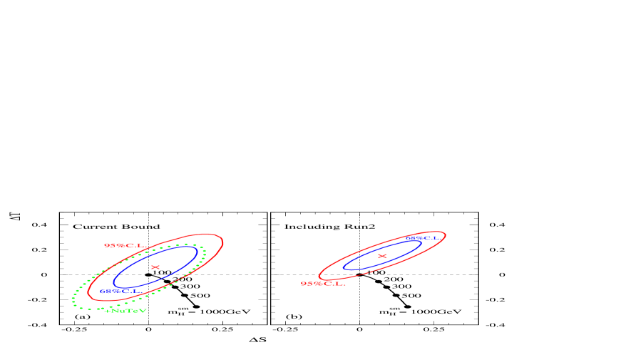
Figure 1: $\Delta S-\Delta T$ contours (a) from the current precision electroweak data, and (b) from including the expected Tevatron Run-2 sensitivity to $m^{~{}}_{W}$ and $m^{~{}}_{t}$ [assuming the current central values of $(m^{~{}}_{W},\,m^{~{}}_{t})$ with an error of $(20\,{\rm MeV},\,2$ GeV)]. Here, we set $m_{H}^{\rm ref}=100$ GeV and $\Delta U=0$ in the global fit. The dotted curve in (a) is the 95% C.L. bound after including the NuTeV data.

If one assumes that there were no new physics beyond the SM, a global fit to the current precision electroweak data would suggest the SM Higgs to be light, with a central value $m^{~{}}_{H}=83$ GeV (significantly below the LEP2 direct search limit $m^{~{}}_{H}>114.3$ GeV [18]) and a 95% C.L. limit on the range of Higgs boson mass: $\,32\,{\rm GeV}\,\leqslant m^{~{}}_{H}\leqslant 192$ GeV.  However, it was recently pointed out that in the presence of new physics, such a bound can be substantially relaxed [19, 20, 21, 22, 23]. In the above fit we did not include the latest NuTeV data. If the NuTeV data is included, the value of the minimum $\chi^{2}$ of the global fit increases substantially (by $8.7$), indicating a poor quality of the SM fit to the precision data. (This fit gives a similar central value,  $m^{~{}}_{H}=85$ GeV,  and 95% C.L. mass range $\,33\,{\rm GeV}\,\leqslant m^{~{}}_{H}\leqslant 200$ GeV.) A similar increase of $\chi^{2}$ (by 8.9) also appears in the $\Delta S-\Delta T$ fits, suggesting that the NuTeV anomaly cannot be explained by the new physics effect arising from the oblique parameters $(\Delta S,\,\Delta T)$ alone. Since the potential problems with the NuTeV analysis are still under debate [24], the NuTeV data will not be included in the following analysis. In Fig. 1(a), we show the $\Delta S-\Delta T$ bounds (setting $m_{H}^{\rm ref}=100$ GeV), derived from the global fits with the newest updated electroweak precision data [25, 26]. Furthermore, for $m_{H}^{\rm ref}=115\,(300)$ GeV and $\Delta U=0$, the global fits give

$$\Delta S=0.01\,(-0.07)\pm 0.09\,,~{}~{}~{}~{}~{}\Delta T=0.07\,(0.16)\pm 0.11\,.$$ (6)

What also shown in the same figure is the contribution to $\Delta S$ and $\Delta T$ from the SM Higgs boson with different masses. Fig. 1(b) shows that the upcoming measurements of the $W^{\pm}$ mass ($m_{W}$) and top mass ($m_{t}$) at the Tevatron Run-2 can significantly improve the constraints on the new physics via the oblique corrections, where the current Run-1 central values of $(m^{~{}}_{W},\,m^{~{}}_{t})$ are assumed, but with their errors reduced to the planned sensitivity of $20$ MeV and $2$ GeV, respectively.

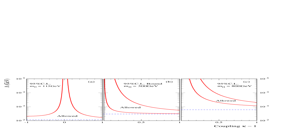
Figure 2: Constraints on the new physics scale $\Lambda$ as a function of the anomalous coupling $\Delta\kappa$. The regions below the solid curves and above the dashed lines in (a) or between the two solid curves in (b)-(c) are allowed at the $95\%$C.L. The dashed lines indicate the value of Higgs mass $m^{~{}}_{H}$.

Given the allowed range of $(\Delta S,\,\Delta T)$, as shown in Fig. 1(a), we can further constrain the new physics scale $\Lambda$ as a function of the anomalous coupling $\Delta\kappa$ for a given $m_{H}^{\rm ref}=m^{~{}}_{H}$ value [cf. Eq.(5)]. The results are depicted in Fig. 2. Alternatively, from Fig. 2, we can constrain the range of $\Delta\kappa$ for given values of $(\Lambda,\,m^{~{}}_{H})$, as summarized in Table 1.

Table 1: The 95% C.L. limits on $\Delta\kappa$ for typical values of new physics scale $\Lambda$ and Higgs mass $m_{H}^{~{}}$.

$\Lambda=$	$1$ TeV	$10$ TeV	$100$ TeV
$m_{H}=115$ GeV	$-0.15\leqslant\Delta\kappa\leqslant 0.23$	$-0.069\leqslant\Delta\kappa\leqslant 0.12$	$-0.045\leqslant\Delta\kappa\leqslant 0.08$
$300$ GeV	$-0.074\leqslant\Delta\kappa\leqslant 0.60$	$0.027\leqslant\Delta\kappa\leqslant 0.24$	$0.016\leqslant\Delta\kappa\leqslant 0.15$
$800$ GeV	(excluded)	$0.20\leqslant\Delta\kappa\leqslant 0.45$	$0.11\leqslant\Delta\kappa\leqslant 0.26$

Fig. 2 and Table 1 show that for $\,m^{~{}}_{H}\gtrsim 250-300$ GeV, the $\,\Delta\kappa<0\,$ region is fully excluded, while a sizable $\,\Delta\kappa>0\,$ is allowed provided $\Lambda$ is relatively low. Furthermore, for $\,m^{~{}}_{H}\gtrsim 800$ GeV, the region $\,\Lambda<1.1$ TeV is excluded. For $\,m^{~{}}_{H}\gtrsim 250-300$ GeV, the preferred range of $\Delta\kappa>0$ requires the couplings of $HW^{+}W^{-}$ and $HZZ$ to be stronger than that of the SM, so that the direct production rate of the Higgs boson, via either the Higgs-strahlung or the $VV$ fusions in high energy collisions, should raise above the SM rate. On the other hand, for $m^{~{}}_{H}\lesssim 250$ GeV, the direct production rate of the Higgs boson can be smaller or larger than the SM rate depending on the sign of $\Delta\kappa$. Thus, when $\Delta\kappa<0$, a light non-standard Higgs boson may be partially hidden by its large SM background events. However, in this case, the new physics scale $\Lambda$ will be generally low. For instance, when $m^{~{}}_{H}=115$ GeV, a negative $\Delta\kappa=-0.15\,(-0.28)$ already forces $\Lambda\leqslant 1\,(0.4)$ TeV. Finally, we note that for certain class of models the new physics may also invoke extra heavy fermions such as in the typical top-seesaw models with new vector-like fermions [19, 1] or models with new chiral families [21]. In that case, there can be generic positive contributions to $\Delta T$, so that the $\Delta\kappa<0$ region may still be allowed for a relatively heavy Higgs boson, but such possibilities are very model-dependent. In our current effective theory analysis, we consider the bosonic $HVV$ couplings as the dominant contributions to the oblique parameters, and assume that other possible anomalous couplings (such as the deviation in the gauge interactions of $tbW/t\bar{t}Z$) may be ignored. However, independent of these assumptions, the most decisive test of the $HVV$ couplings can come from direct measurements via Born-level processes at the high energy colliders, which is the subject of the next two sections.

3 . Probing $HVV$ Interaction from Weak Boson Scattering

When a light Higgs boson (less than about $300$ GeV) is detected, the anomalous coupling $\kappa$ may be measured from the production and the decay of the Higgs boson (cf. next section). Moreover, it is important to study the weak-boson scatterings in the TeV region and test whether this Higgs boson is truly responsible for the mechanism of the spontaneous EWSB, i.e., for generating the longitudinally polarized weak bosons (and their observed masses). Consider the effective Lagrangian (1). When $\kappa=1$, the weak gauge boson scatterings in the TeV region will be dominated by the transversely polarized weak bosons (denoted as $V_{T}$) and the scattering amplitudes will be small when the Higgs boson is light. However, when $\kappa\neq 1$ and $|\Delta\kappa|={\cal O}(1)$, the weak boson scatterings in the TeV regime will be dominated by the longitudinally polarized weak bosons (denoted as $V_{L}$) and the scattering amplitudes will grow as the invariant mass of the weak boson pair (denoted as $E$) increases. Applying the electroweak power counting method [27], we find that the $V_{T}V_{T}$ scattering amplitude behaves as  $g^{2}\kappa^{2}E^{0}$  and the $V_{L}V_{L}$ scattering amplitude rapidly grows as  $(\kappa^{2}-1)E^{2}/v^{2}$.  For a large $E$ and $\Delta\kappa\neq 0$, the $V_{L}V_{L}$ scattering can dominate the $VV\rightarrow VV$ processes, and the growth of the event rate can sensitively probe the deviation $\Delta\kappa$.

As shown in Fig. 2, for $m^{~{}}_{H}\gtrsim 250-300$ GeV, the precision electroweak data already exclude a negative $\Delta\kappa$. Hence, if new physics effect sets in the $HVV$ coupling $\kappa=1+\Delta\kappa$, the production rates of $VH$ and $qq\rightarrow qqH$, and the total decay width of $H$ should raise above the SM predictions. It can be the case that for a sizable $\Delta\kappa>0$, the total width of $H$ becomes so large that $H$ cannot be detected as a sharp resonance [28] and therefore escapes the detection when scanning the invariant mass of its decay products around $m^{~{}}_{H}$ region. In this case, can we still probe such a sub-TeV Higgs boson? The answer is yes: as explained above, it unavoidably leads to enhanced $VV$-scattering amplitudes of ${\cal O}\!\left((\kappa^{2}-1)E^{2}/v^{2}\right)$ in the TeV region, detectable at the LHC. On the other hand, if $\Delta\kappa$ is considerably negative, the on-shell production rate of a light Higgs boson via Higgs-strahlung or $VV$ fusion becomes so small that it may escape the detections under these channels. However, in this case, the $V_{L}V_{L}$ scattering amplitude has to still grow up with $E^{2}$ and become large at the TeV scale due to the anomalous $\Delta\kappa$ coupling! Therefore, even if a light Higgs boson exists, studying the $VV$ scattering in the TeV regime remains important for testing the true nature of its gauge interactions and the origin of the spontaneous EWSB. Based upon the above observations, we propose to directly test the anomalous coupling $\Delta\kappa$ by studying $VV$ scatterings in the TeV region at the LHC. We will show that rather sensitive tests of $\Delta\kappa$ can be performed by measuring the cross sections of the longitudinal weak-boson scattering, $V_{L}V_{L}\rightarrow V_{L}V_{L}$, especially $W^{+}_{L}W^{+}_{L}\rightarrow W^{+}_{L}W^{+}_{L}$.

The scattering amplitude of $VV\rightarrow VV$ contains two parts: (i) the amplitude $T(V,\gamma)$ related solely to electroweak gauge bosons, and (ii) the amplitude $T(H)$ related to the Higgs boson exchanges. In the SM ($\kappa=1$), the $HVV$ vertex contains the same gauge coupling as in the non-Abelian interaction of the weak bosons. At high energies, both $T(V,\gamma)$ and $T(H)$ grow with $E^{2}$. However, for $\kappa=1$, the $E^{2}$-dependent pieces in the two amplitudes precisely cancel in the sum $T(V,\gamma)+T(H)$ so that the total amplitude only has $E^{0}$-dependence, respecting the unitarity of the $S$-matrix. For the non-standard Higgs boson, $\kappa\neq 1$ originates from the new physics above $\Lambda$, and the two $E^{2}$-dependent pieces do not cancel, making the total amplitude grow as $\,(\kappa^{2}-1)E^{2}/v^{2}\,$ in the region below $\Lambda$. Such anomalous $E^{2}$-behavior (rather than $E^{0}$-behavior of the SM amplitude) occurs only in the $V_{L}V_{L}\rightarrow V_{L}V_{L}$ channel and is rather sensitive to $\Delta\kappa$ .

To analyze the LHC sensitivity to probing the anomalous $HVV$ coupling, we compute the cross sections for $pp\rightarrow jjVV$ numerically using the parton distribution functions CTEQ6L [29]. We consider only the gold-plated (pure leptonic decay) modes of the final state $V$’s in order to avoid the large hadronic backgrounds at the LHC. Even in this case, there are still several classes of large backgrounds to be eliminated, including the electroweak (EW) background, the QCD background, and the top quark background studied in Refs. [30, 31]. Following Refs. [30, 31], we require forward-jet tagging, central-jet vetoing and detecting isolated leptons, nearly back to back, with large transverse momentum in the central rapidity region to suppress the backgrounds. Since we compute the exact tree-level amplitudes of $pp\rightarrow jjVV$ without invoking the effective-$W$ approximation (EWA), our numerical results are valid not only for large $|\Delta\kappa|$ values but also for small $|\Delta\kappa|$ region where the $V_{L}$-contribution to $VV$-scatterings becomes comparable or smaller than that of $V_{T}$ (for $m_{H}\lesssim 300$ GeV) and the signal detection is much harder.

Following the above procedures, we compute the tree-level cross sections of the scattering processes  $pp(VV)\rightarrow VVjj\rightarrow\ell\ell\ell\ell jj$.  We find that the most sensitive channel to determine $\Delta\kappa$ is  $W^{+}_{L}W^{+}_{L}\rightarrow W^{+}_{L}W^{+}_{L}$  due to its small background rates. In Table 2, we summarize the number of events (including both signals and backgrounds) for this most sensitive channel  $pp\rightarrow W^{+}W^{+}jj\rightarrow\ell^{+}\nu\ell^{+}\nu jj$ in the range of  $-0.4\leqslant\Delta\kappa\leqslant 0.4$  and  $115\,{\rm GeV}\leqslant m_{H}\leqslant 300\,{\rm GeV}$,  with an integrated luminosity of 300 fb^-1.

Table 2: Number of events at the LHC (300 fb^-1) for  $pp\rightarrow W^{+}W^{+}jj\rightarrow\ell^{+}\nu\ell^{+}\nu jj$  ($\ell=e,\mu$) with various values of $m^{~{}}_{H}$ (GeV) and $\Delta\kappa$ in the non-standard Higgs model, where $\Delta\kappa=0$ corresponds to the SM. Values of the statistical significance $\,{\cal N}_{S}/\sqrt{{\cal N}_{B}}$  are shown in the parentheses.

$\Delta\kappa=$	$-0.40$	$-0.30$	$-0.24$	$-0.21$	$-0.18$	$0.00$	$0.18$	$0.21$	$0.23$	$0.30$	$0.40$
$m_{H}^{~{}}=$ 115	34(4.9)	27(3.1)	23(2.1)	21(1.5)	19(1.0)	15	23(2.1)	25(2.6)	27(3.1)	37(5.7)	58(11)
130	34(4.9)	27(3.1)	23(2.1)	21(1.5)	19(1.0)	15	23(2.1)	25(2.6)	27(3.1)	37(5.7)	57(11)
200	35(5.2)	28(3.4)	24(2.3)	23(2.1)	21(1.5)	15	20(1.3)	23(2.1)	25(2.6)	33(4.6)	52(9.6)
300	36(5.0)	30(3.5)	26(2.5)	24(2.0)	23(1.8)	16	19(0.8)	22(1.5)	23(1.8)	29(3.3)	43(6.8)

From our analysis, we find that the kinematic cuts of Ref. [30] can effectively suppress the backgrounds relative to the signal for the case with $\Delta\kappa$ significantly different from zero since the $E^{2}$-dependence of the $W_{L}W_{L}$ amplitude enhances the signal. However, for $\Delta\kappa$ close to zero, only the QCD and top quark backgrounds are negligibly small, while the EW background is still quite large compared to the signal. For instance, when $\Delta\kappa=0$, we see that the ${15\sim 16}$ SM-events for $m_{H}\leqslant 300$ GeV in Table 2 come essentially from the $W_{T}W_{L}$ and $W_{T}W_{T}$ contributions (EW backgrounds). So, under these cuts, the real background events are given by,  ${{\cal N}}_{B}={\cal N}[\Delta\kappa=0]={15\sim 16}$ .  We can then define the signal events for $\Delta\kappa\neq 0$ as  ${{\cal N}}_{S}={\cal N}[\Delta\kappa\neq 0]-{{\cal N}}_{B}$ .  To see the sensitivity of the LHC for discriminating the cases between $\Delta\kappa\neq 0$ and $\Delta\kappa=0$ (SM), we also show the statistical significance  ${\cal N}_{S}/\sqrt{{\cal N}_{B}}$  in the parentheses in Table 2. The values of $\Delta\kappa$ corresponding to the $2\sigma$ level of deviations from the SM are explicitly displayed in Table 2. Hence, if the $\Delta\kappa\neq 0$ effect is not detected, the LHC can constrain the range of $\Delta\kappa$ to be about

$$-0.2~{}<~{}\Delta\kappa~{}<~{}0.2\,,$$ (7)

at the $2\sigma$ level.

Before concluding this section, we discuss the possible unitarity violation in the scattering process  $pp\rightarrow W^{+}W^{+}jj\rightarrow\ell\nu\ell\nu jj$ (for $\kappa\neq 1$), whose leading contribution comes from the sub-process $W^{+}_{L}W^{+}_{L}\rightarrow W^{+}_{L}W^{+}_{L}$ when the initial $W_{L}^{+}W_{L}^{+}$ are almost collinearly radiated from the incoming quarks or antiquarks. The scattering amplitude of $W^{+}_{L}W^{+}_{L}\rightarrow W^{+}_{L}W^{+}_{L}$ contributes to the isospin $I=2$ channel, and in the high energy region ($E^{2}\gg M^{2}_{W},m^{2}_{H}$), is dominated by the leading $E^{2}$-contributions, $\,T[I=2]\simeq(\kappa^{2}-1)E^{2}/v^{2}$.  According to the partial-wave analysis, its $s$-wave amplitude  $a^{~{}}_{I,J=2,0}$  is given by

$$a^{~{}}_{20}~{}\simeq~{}\displaystyle\left(\kappa^{2}-1\right)\frac{E^{2}}{\,16\pi v^{2}\,}\,,$$ (8)

where $E=M_{VV}$. The unitarity condition for this channel is, $\,|\Re\mathfrak{e}\,a^{~{}}_{20}|<{2!}/{2}=1$ ,  and the factor $2!$ is due to the identical $W^{+}W^{+}$ in the final state. This results in a requirement,

$$\sqrt{1-\frac{\,16\pi v^{2}\,}{E^{2}}}~{}<~{}|\kappa|~{}<~{}\sqrt{1+\frac{\,16\pi v^{2}\,}{E^{2}}}\,.$$ (9)

For instance, it constrains  $|\kappa|<3.6$  for  $E=500$ GeV,  and  $0.5\,(0.8)<|\kappa|<1.3\,(1.2)$  for  $E=2\,(3)$ TeV.  Hence, the expected sensitivity of the LHC to determining $\Delta\kappa$ [cf. Eq. (7)] is consistent with the unitarity limit since the typical invariant mass of the $W^{+}W^{+}$ pair, after the kinematic cuts, falls into the range  $500\,{\rm GeV}\leqslant E\leqslant 2\sim 3$ TeV. The contributions from higher invariant mass values are severely suppressed by the parton luminosities [30, 27] and thus negligible.

4 . Other Measurements

The anomalous $HVV$ coupling can also be measured from the associate production of the Higgs boson with the weak boson, as well as the total decay width of the Higgs boson.

4.1 . Constraints from the $VH$ Associate Production

The anomalous $HVV$ coupling can be directly measured via the associate $VH$ production in the lepton or hadron collisions, $\,e^{-}e^{+},\,q{q^{\prime}}\rightarrow VH$. The LEP-2 Higgs search puts a direct bound, $m_{H}^{\rm SM}>114.3$ GeV [18]. For a non-SM Higgs boson, this lower bound can be weakened. For instance, in the supersymmetric SM, the $HZZ$ coupling is smaller than its SM value by a factor $\sin(\alpha-\beta)$ or $\cos(\alpha-\beta)$, depending on whether $H$ is the lighter or heavier CP-even state, and this lower bound is reduced to about 90 GeV [18]. If the SM Higgs boson weighs about 110 GeV, Tevatron Run-2 will be able to detect it. Assuming an integrated luminosity of $10\,{\rm fb}^{-1}$, the number of expected signal events is about 27 and the background events about 258, according to the Table 3 (the most optimal scenario) of Ref. [32]. Therefore, the $1\sigma$ statistic fluctuation of the background event is about $16$. Consequently, we find, at the $1\sigma\,(2\sigma)$ level,  $0.6<|\kappa|<1.2$ ($|\kappa|<1.5$) .  Similarly, we can estimate the bounds on $|\kappa|$ for various $m^{~{}}_{H}$ values as below

$$\begin{array}[]{rcc}&1\sigma{}&2\sigma{}{}{}\\[4.2679pt] m_{H}^{~{}}=110~{}{\rm GeV:}&~{}~{}~{}0.6\leqslant|\kappa|\leqslant 1.2\,,{}{}{}&0\leqslant|\kappa|\leqslant 1.5\,;\\[2.84526pt] m_{H}^{~{}}=120~{}{\rm GeV:}&0.4\leqslant|\kappa|\leqslant 1.4\,,&0\leqslant|\kappa|\leqslant 1.6\,;\\[2.84526pt] m_{H}^{~{}}=130~{}{\rm GeV:}&~{}~{}0\leqslant|\kappa|\leqslant 1.5\,,&0\leqslant|\kappa|\leqslant 1.8\,.\\ \end{array}$$ (10)

It is clear that the above limits can be further improved at the Tevatron Run-2 by having a larger integrated luminosity until the systematical error dominates over the statistical error. The same process can also be studied at the LHC to test the anomalous coupling $\kappa$. However, because of much larger background rate at the LHC, the improvement on the measuring $\kappa$ via the $VH$ associate production is not expected to be significant.

4.2 . Constraints from Decay Width of Higgs Boson

Another method to determine $\kappa$ is to measure the decay width of the Higgs boson. When  $m^{~{}}_{H}>2m^{~{}}_{Z}$,  the decay process $\,H\rightarrow ZZ\rightarrow 4\mu$  is one of the “gold-plated” channels (the pure leptonic decay modes) that allow the reconstruction of the $ZZ$ invariant mass with a high precision. Thus, the total decay width of the Higgs boson can be precisely measured. A detailed Monte Carlo analysis for such a measurement at the LHC was carried out in Ref. [33]. Assuming that there is no non-SM decay channel open except the presence of the anomalous $HVV$ coupling $\kappa$, we can directly convert the results of Ref. [33] to the limits on $\kappa$. Since the decay branching ratios of $H\rightarrow W^{+}W^{-}/ZZ$ for the SM Higgs boson become dominant when $m_{H}^{~{}}\gtrsim 200$ GeV, the total width measurement can impose a strong constraint on $\kappa$. From the Table 3 of Ref. [33], we can derive the accuracy on the determination of $\kappa$ from the relation $-n\Delta\Gamma\leq\Gamma(\kappa)-\Gamma(\kappa=1)\leq n\Delta\Gamma$, where $n=1,2$ denote the $1\sigma$ and $2\sigma$ accuracy, respectively, $\Gamma(\kappa)$ is the Higgs width for a given value of $\kappa$, $\Gamma(\kappa=1)$ is the SM Higgs width and $\Delta\Gamma$ is the expected experimental error of the width measurement. We find that at the LHC (with an integrated luminosity of $300\,{\rm fb}^{-1}$), measuring the total Higgs decay width via  $pp\rightarrow H\rightarrow ZZ\rightarrow 4\mu$  can constrain $\kappa$ as

$$\begin{array}[]{lcc}{1\sigma\!:}~{}~{}~{}0.9\,\leqslant~{}|\kappa|~{}\,\leqslant 1.1\,,{}{}&~{}~{}{2\sigma\!:}~{}~{}~{}0.8\,\leqslant~{}|\kappa|~{}\,\leqslant 1.2\,,~{}~{}~{}~{}~{}({\rm for}~{}m_{H}^{~{}}=200\!-\!300\,{\rm GeV}).\end{array}$$ (11)

Before closing this section, a few remarks are in order. First, when the Higgs boson is lighter than $2m_{Z}^{~{}}$, it is expected that the production rate of $qq\rightarrow qqH$ with $H\rightarrow WW^{*}\rightarrow\ell\ell^{\prime}{\not\!\!E_{T}}$ is large enough to be detected at the LHC and the $HWW$ coupling can be determined by studying the observables near the Higgs boson resonance [34]. Similarly, at the future Linear Colliders, the anomalous $HZZ$ coupling can be measured via  $e^{-}e^{+}\rightarrow ZH(\rightarrow b\bar{b})$ [35]. The implication of these measurements to the determination of $\kappa$ will be presented elsewhere [13]. Finally, another important effect of an anomalous $\Delta\kappa$ is to modify the decay branching ratio of  $H\rightarrow\gamma\gamma$,  and consequently, the production rate of  $gg\rightarrow H\rightarrow\gamma\gamma$  at the LHC. As a function of $\kappa$, Br$[H\rightarrow\gamma\gamma]$ decreases when $\kappa$ is moving above $1$, and increases otherwise [13].

5 . Conclusions

In this work, we studied the constraints on the anomalous $HVV$ coupling $\Delta\kappa$ from the latest precision electroweak data and from the high energy $V_{L}V_{L}$ scatterings at the upcoming LHC experiments. Comparisons were also made with the other limits derived from the associate production rate of $VH$ and the total decay width of the Higgs boson. We showed that the existing precision data already impose nontrivial constraints on the allowed ranges of $\Delta\kappa$ and the new physics scale $\Lambda$ (cf. Fig. 2 and Table 1). We further demonstrated that the $V_{L}V_{L}$ scatterings, especially $W^{+}_{L}W^{+}_{L}\rightarrow W^{+}_{L}W^{+}_{L}$ channel, can sensitively test $\Delta\kappa$ at the LHC, with an integrated luminosity of about $300$ fb^-1 (cf. Table 2). Hence, $V_{L}V_{L}$ scatterings are not only important for probing strongly interacting EWSB mechanism [7, 30, 27] when there is no light Higgs boson, but also valuable for testing the anomalous $HVV$ interactions when the Higgs boson is relatively light. It is particularly important when a positive $\Delta\kappa$ causes a broad Higgs resonance that may be hidden by its backgrounds, or when a negative $\Delta\kappa$ makes the production rate of a light Higgs boson too small to be detected near the Higgs resonance. In either case, because a SM Higgs boson would perfectly saturate the unitarity, the enhanced $V_{L}V_{L}$-scattering signals in the TeV region directly test the anomalous $HVV$ couplings and thus probe the underlying EWSB mechanism.

The classic “no-lose” theorem asserts that the LHC, capable of observing the $V_{L}V_{L}$ scatterings at $1-2$ TeV scale, will not fail to test the EWSB mechanism [7]. Our study provides a new support of this theorem by showing that even if there exists a Higgs boson as light as $115-300$ GeV and some of its on-shell production channels may be hard to detect, the $V_{L}V_{L}$ scatterings at the LHC can still become strong in the TeV regime due to the anomalous $HVV$ interactions. To further discriminate such a non-standard light Higgs boson from a strongly interacting EWSB sector with no light resonance will eventually demand a multi-channel analysis at the LHC by searching for the light resonance through all possible on-shell production channels, including the gluon-gluon fusion (unless its interactions with heavy quarks, such as the top and bottom quarks, are highly suppressed). Indeed, the physics with unraveling the EWSB mechanism could be much more intricate than naively expected, and studying the $VV$ scatterings at TeV scale is important for guiding the light Higgs searches via its on-shell production, as well as for testing the EWSB mechanism via $HVV$ interactions after a light Higgs resonance is found.

Acknowledgements     We thank J. Bagger, R. S. Chivukula, P. B. Renton and especially J. Erler for discussing the precision data, and D. Zeppenfeld for discussing the weak boson physics of the LHC. This work was supported by the U.S. DOE grant DE-FG0393ER40757 and NSF grant PHY-0100677, and by the NSF of China and Tsinghua Foundation of Fundamental Research.

References

- [1] For an updated comprehensive review, C. T. Hill and E. H. Simmons, hep-ph/0203079.
- [2] For recent reviews, H. E. Haber, hep-ph/0212136; and “Perspectives on Supersymmetry”, ed. G. L. Kane, World Scientific Publishing Co., 1998.
- [3] N. Arkani-Hamed, S. Dimopolous, G. R. Dvali, Phys. Lett. B429 (1998) 263; I. Antoniadis, N. Arkani-Hamed, S. Dimopolous, G. R. Dvali, Phys. Lett. B436 (1998) 257; L. Randall and R. Sundrum, Phys. Rev. Lett. 83 (1999) 3370.
- [4] D. B. Kaplan and H. Georgi, Phys. Lett. B136 (1984) 183.
- [5] E.g., T. Rizzo and J. D. Wells, Phys. Rev. D61 (1999) 016007 and references therein.
- [6] N. Arkani-Hamed, A. G. Cohen, and H. Georgi, Phys. Lett. B513 (2001) 232.
- [7] M. S. Chanowitz and M. K. Gaillard, Nucl. Phys. B261 (1985) 379; Michael S. Chanowitz, Lecture at Zuoz Summer School [hep-ph/9812215] and references therein.
- [8] C. G. Callen, S. Coleman, J. Wess and B. Zumino, Phys. Rev. 177 (1969) 2247.
- [9] S. Weinberg, Physica A96 (1979) 327.
- [10] T. Appelquist and C. Bernard, Phys. Rev. D22 (1980) 200; A. C. Longhitano, Nucl. Phys. B188 (1981) 118.
- [11] R. Sekhar Chivukula and V. Koulovassilopoulos, Phys. Lett. B309 (1993) 371.
- [12] W. Buchmüller and D. Wyler, Nucl. Phys. B268 (1986) 621.
- [13] B. Zhang, Y.-P. Kuang, H.-J. He, C.-P. Yuan, in preparation.
- [14] A. Manohar and H. Georgi, Nucl. Phys. B234 (1984) 189; H. Georgi, Phys. Lett. B298 (1993) 187 [hep-ph/9207278].
- [15] M. E. Peskin and T. Takeuchi, Phys. Rev. Lett. 65 (1990) 964; Phys. Rev. D46 (1992) 381.
- [16] E.g., S. Dawson and G. Valencia, Nucl. Phys. B439 (1995) 3.
- [17] H. Georgi, Ann. Rev. Nucl. & Part. Sci. 43 (1994) 209, and references therein.
- [18] Particle Data Group (K. Hagiwara et al.), Phys. Rev. D 66 (2002) 010001.
- [19] B. A. Dobrescu, C. T. Hill, Phys. Rev. Lett. 81 (1998) 2634; R. S. Chivukula, B. A. Dobrescu, H. Georgi, C. T. Hill, Phys. Rev. D59 (1999) 075003; H.–J. He, C. T. Hill, T. Tait, Phys. Rev. D65 (2002) 055006; H.–J. He, T. Tait, C.–P. Yuan, Phys. Rev. D62 (2000) 011702 (R).
- [20] J. Bagger, A. F. Falk and M. Swartz, Phys. Rev. Lett. 84 (2000) 1385; R. S. Chivukula, C. Holbling and N. Evans, Phys. Rev. Lett. 85 (2000) 511; C. Kolda and H. Murayama, JHEP 0007 (2000) 035; M. E. Peskin and J. D. Wells, Phys. Rev. D64 (2001) 093003.
- [21] H.–J. He, N. Polonsky and S. Su, Phys. Rev. D64 (2001) 053004 [hep-ph/0102144].
- [22] R. Sekhar Chivukula and C. Holbling, Snowmass contribution [hep-ph/0110214].
- [23] M. S. Chanowitz, Phys. Rev. D66 (2002) 073002 [hep-ph/0207123].
- [24] E.g., G. A. Miller and A. W. Thomas, hep-ex/0204007; S. Davidson, hep-ph/0209316.
- [25] J. Erler, private communications, hep-ph/0005084 and review at http://pdg.lbl.gov.
- [26] M. W. Grünewald, talk at ICHEP, Amsterdam, July 24-31, 2002 [hep-ex/0210003]; see also, P. B. Renton, Rept. Prog. Phys. 65 (2002) 1271 [hep-ph/0206231].
- [27] H.–J. He, Y.–P. Kuang and C.–P. Yuan, Phys. Rev. D55 (1997) 3038 [hep-ph/9611316]; Phys. Lett. B382 (1996) 149 [hep-ph/9604309]; and review in DESY-97-056 [hep-ph/9704276].
- [28] R. S. Chivukula, M. J. Dugan, M. Golden, Phys. Lett. B336 (1994) 62 [hep-ph/9406281].
- [29] J. Pumplin, et al., JHEP 0207 (2002) 012 [hep-ph/0201195].
- [30] J. Bagger, V. Barger, K. Cheung, J. Gunion, T. Han, G. Ladinsky, R. Rosenfeld, C.–P. Yuan, Phys. Rev. D52 (1995) 3878 [hep-ph/9504426].
- [31] C.–P. Yuan, Proposals for Studying TeV Interactions Experimentally, [hep-ph/9712513], in Perspectives on Higgs Physics, G. L. Kane (Ed.), World Scientific Pub.
- [32] P. Agrawal, Mod. Phys. Lett. A16 (2001) 897 [hep-ph/0011347].
- [33] V. Drollinger and A. Sopczak, in the proceedings of LCWS-2001 [hep-ph/0102342].
- [34] D. Zeppenfeld, Snowmass contribution [hep-ph/0203123] and references therein.
- [35] E.g., K. Hagiwara, et al., Eur. Phys. J. 14 (2000) 457, and references therein.