Abstract

We evaluate the relic density of neutralinos in the minimal supergravity (mSUGRA) model. All $2\rightarrow 2$ neutralino annihilation diagrams, as well as all initial states involving sleptons, charginos, neutralinos and third generation squarks are included. Relativistic thermal averaging of the velocity times cross sections is performed. We find that co-annihilation effects are only important on the edges of the model parameter space, where some amount of fine-tuning is necessary to obtain a reasonable relic density. Alternatively, at high $\tan\beta$, annihilation through the broad Higgs resonances gives rise to an acceptable neutralino relic density over broad regions of parameter space where little or no fine-tuning is needed.

1 Introduction

A wide variety of astrophysical measurements are being used to pin down some of the basic cosmological parameters of the universe. High resolution maps of the cosmic microwave background (CMB) radiation[1] imply that the energy density of the universe $\Omega=\rho/\rho_{c}\simeq 1$, consistent with inflationary cosmology. Here, $\rho_{c}=3H^{2}/8\pi G_{N}$ is the critical closure density of the universe, where $G_{N}$ is Newton’s constant and $H=100h$ km/sec/Mpc is the scaled Hubble constant. The value of $h$ itself is determined to be $\sim 0.7\pm 0.1$ by improved measurements of distant galaxies[2]. Meanwhile, data from distant supernovae[3] imply a nonzero dark energy content of the universe $\Omega_{\Lambda}\sim 0.7$, a result which is confirmed by fits to the CMB power spectrum[4]. Analyses of Big Bang nucleosynthesis[5] imply the baryonic density $\Omega_{b}h^{2}\simeq 0.020\pm 0.002$, although the CMB fits suggest a somewhat higher value of $\sim 0.03$. Hot dark matter, for instance from massive neutrinos, should give only a small contribution to the total matter density of the universe. In contrast, a variety of data ranging from galactic rotation curves to large scale structure and the CMB imply a significant density of cold dark matter (CDM)[6] $\Omega_{c}h^{2}\simeq 0.2\pm 0.1$.

In many $R$-parity conserving supersymmetric models of particle physics, the lightest neutralino ($\widetilde{Z}_{1}$) is also the lightest SUSY particle (LSP); as such, it is massive, neutral and stable. For this case, relic neutralinos left over from the Big Bang provide an excellent candidate for the CDM content of the universe[7]. In this work, we present results of calculations of the neutralino relic density within the context of the paradigm minimal supergravity model (mSUGRA, or CMSSM)[8]. In mSUGRA, it is assumed that SUSY breaking occurs in a hidden sector of the model, with SUSY breaking effects communicated from hidden to observable sectors via gravitational interactions. The model parameter space is given by

$$m_{0},\ m_{1/2},\ A_{0},\ \tan\beta\ {\rm and}\ sign(\mu).$$ (1)

Here, $m_{0}$ is the universal scalar mass, $m_{1/2}$ is the universal gaugino mass and $A_{0}$ is the universal trilinear mass all evaluated at $M_{GUT}$, while $\tan\beta$ is the ratio of Higgs field vevs ($v_{u}/v_{d}$), and $\mu$ is a supersymmetric Higgs mass term. The soft SUSY breaking parameters, along with gauge and Yukawa couplings, evolve from $M_{GUT}$ to $M_{weak}$ according to their renormalization group (RG) equations. At $M_{weak}$, the RG improved 1-loop effective potential is minimized, and electroweak gauge symmetry is broken radiatively. In this report, we implement the mSUGRA solution encoded in ISAJET v7.64[9].

There is a long history of increasingly sophisticated solutions for the relic density of neutralinos in supersymmetric models[10, 11, 12, 13, 14, 15, 16, 17, 18, 19, 20, 21, 22, 23, 24, 25, 26, 27, 28, 29, 30, 31, 32, 34, 35]. The key ingredient to solving the Boltzmann equation is to evaluate the thermally averaged neutralino annihilation cross section times velocity factor. Traditionally, the solution is made by expanding the annihilation cross section as a power series in neutralino velocity, so that angular and energy integrals can be evaluated analytically. The remaining integral over temperature can then be performed numerically. The power series solution is valid in many regions of model parameter space because the relic neutralino velocity is expected to be highly non-relativistic.

However, it was emphasized by Griest and Seckel that annihilations may occur through $s$-channel resonances at high enough energies[14] that a relativistic treatment of thermal averaging might be necessary. Drees and Nojiri found that at large values of the parameter $\tan\beta$, neutralino annihilation can be dominated by $s$-channel scattering through broad $A$ and $H$ Higgs resonances[17]. The proper formalism for relativistic thermal averaging was developed by Gondolo and Gelmini (GG)[15], and was implemented in the code of Baer and Brhlik[20, 22]. Working within the framework of the mSUGRA model, it was found[20, 22, 23, 29, 30] that at large $\tan\beta$, indeed large new regions of model parameter space gave rise to reasonable values for the CDM relic density. At large $\tan\beta$, the $A$ and $H$ resonances are broad enough (typically 10-50 GeV) that even if the quantity $2m_{\widetilde{Z}_{1}}$ is several partial widths away from exact resonance, there can still be a significant rate for neutralino annihilation. Thus, in the mSUGRA model at low $m_{0}$ and $\tan\beta$, neutralino annihilation is dominated by $t$-channel slepton exchange, and reasonable values of the relic density occur only for relatively low values of $m_{0}$ and $m_{1/2}$. At high $\tan\beta$, a much larger parameter space is allowed, owing to off-resonance neutralino annihilation through the broad Higgs resonances.

In addition, there exist regions of mSUGRA model parameter space where co-annihilation processes are important, and even dominant. It was stressed by Griest and Seckel[14] that in regions with a higgsino-like LSP, the $\widetilde{Z}_{1}$, $\widetilde{W}_{1}$ and $\widetilde{Z}_{2}$ masses become nearly degenerate, so that all three species can exist in thermal equilibrium, and annihilate against one another. The relativistic thermal averaging formalism of GG was extended to include co-annihilation processes by Edsjö and Gondolo[21], and was implemented in the DarkSUSY code[24] for co-annihilation of charginos and heavier neutralinos.

The importance of neutralino-slepton co-annihilation was stressed by Ellis et al. and others[26, 27, 28, 29, 30]. In regions of mSUGRA parameter space where $\widetilde{Z}_{1}$ and $\tilde{\tau}_{1}$ (or other sleptons) were nearly degenerate (at low $m_{0}$), co-annihilations could give rise to reasonable values of the relic density even at very large values of $m_{1/2}$, at both low and high $\tan\beta$. In addition, for large values of the parameter $A_{0}$ or for non-universal scalar masses, top or bottom squark masses could become nearly degenerate with the $\widetilde{Z}_{1}$, so that squark co-annihilation processes can become important as well[31, 32].

The goal of this study is to calculate the relic density of neutralinos in the mSUGRA model including co-annihilation processes in addition to relativistic thermal averaging of the annihilation cross section times velocity. Since there are very many Feynman diagrams to evaluate for neutralino annihilations and co-annihilations, we use CompHEP v.33.23[33], which provides for fast and efficient automatic evaluation of tree level processes in the SM or MSSM. For initial states including $\widetilde{Z}_{1}$, $\widetilde{Z}_{2}$, $\widetilde{W}_{1}$, $\tilde{e}_{1}$, $\tilde{\mu}_{1}$, $\tilde{\tau}_{1}$, $\tilde{t}_{1}$ and $\tilde{b}_{1}$, we count 1722 subprocesses, including 7618 Feynman diagrams. For those processes we have calculated the squared matrix element and have written it down in the form of CompHEP FORTRAN output.

The weak scale parameters from supersymmetric models are generated using ISAJET v7.64, and interfaced with the squared matrix elements from CompHEP. Details of our computational algorithm are given in Sec. 2. In Sec. 3 we present a variety of results for the relic density in mSUGRA model parameter space. Much of parameter space is ruled out at low $\tan\beta$ since the relic density is too high, and would yield too small an age of the universe. At high $\tan\beta$, large regions of parameter space are available with a reasonable relic density in the range $0.1<\Omega_{\widetilde{Z}_{1}}h^{2}<0.3$. In Sec. 4, we conclude.

2 Calculational Details

The evolution of the number density of supersymmetric relics in the universe is described by the Boltzmann equation as formulated for a Friedmann-Robertson-Walker universe. For calculations including many particle species, such as the case where co-annihilations are important, there is a Boltzmann equation for each particle species. Following Griest and Seckel[14], the equations can be combined to obtain a single equation

$$\frac{dn}{dt}=-3Hn-\langle\sigma_{eff}v\rangle\left(n^{2}-n_{eq}^{2}\right),\ \mbox{where \ \ }n=\sum_{i=1}^{N}n_{i}$$ (2)

and the sum extends over the $N$ particle species contributing to the relic density, with $n_{i}$ being the number density of the $i$th species. Furthermore, $n_{eq,i}$ is the number density of the $i$th species in thermal equilibrium, given by

$$n_{eq,i}=\frac{g_{i}m_{i}^{2}T}{2\pi^{2}}K_{2}\left(\frac{m_{i}}{T}\right),$$ (3)

where $K_{j}$ is a modified Bessel function of the second kind of order $j$.

The quantity $\langle\sigma_{eff}v\rangle$ is the thermally averaged cross section times velocity. A succinct expression for this quantity using relativistic thermal averaging was computed by Gondolo and Gelmini for the case of a single particle species[15], and was extended by Edsjö and Gondolo for the case including co-annihilations[21]. We adopt this latter form, given by

$$\langle\sigma_{eff}v\rangle(x)=\frac{\int_{2}^{\infty}K_{1}\left({a\over x}\right)\sum_{i,j=1}^{N}\lambda(a^{2},b_{i}^{2},b_{j}^{2})g_{i}g_{j}\sigma_{ij}(a)da}{4x\left(\sum_{i=1}^{N}K_{2}\left({b_{i}\over x}\right)b_{i}^{2}g_{i}\right)^{2}},$$ (4)

where $x=T/m_{\widetilde{Z}_{1}}$ is the temperature in units of mass of the relic neutralino, $\sigma_{ij}$ is the cross section for the annihilation reaction $ij\rightarrow X$ ($X$ is any allowed final state consisting of 2 SM and/or Higgs particles), $\lambda(a^{2},b_{i}^{2},b_{j}^{2})=a^{4}+b_{i}^{4}+b_{j}^{4}-2(a^{2}b_{i}^{2}+a^{2}b_{j}^{2}+b_{i}^{2}b_{j}^{2})$, $a=\sqrt{s}/m_{\widetilde{Z}_{1}}$ and $b_{i}=m_{i}/m_{\widetilde{Z}_{1}}$. This expression is our master formula for the relativistically thermal averaged annihilation cross section times velocity.

To solve the Boltzmann equation, we introduce a freeze-out temperature $T_{F}$, so that the relic density of neutralinos is given by

$$\Omega_{\widetilde{Z}_{1}}h^{2}=\frac{\rho(T_{0})}{8.1\times 10^{-47}\ {\rm GeV}^{4}}$$ (5)

where

$$\rho(T_{0})\simeq 1.66{1\over M_{Pl}}\left(\frac{T_{m_{\widetilde{Z}_{1}}}}{T_{\gamma}}\right)^{3}T_{\gamma}^{3}\sqrt{g_{*}}\frac{1}{\int_{0}^{x_{F}}\langle\sigma_{eff}v\rangle dx}.$$ (6)

The freeze-out temperature $x_{F}=T_{F}/m_{\widetilde{Z}_{1}}$ is determined as usual by an iterative solution of the freeze-out relation

$$x_{F}^{-1}=\log\left[\frac{m_{\widetilde{Z}_{1}}}{2\pi^{3}}\frac{g_{eff}}{2}\sqrt{\frac{45}{2g_{*}G_{N}}}\langle\sigma_{eff}v\rangle(x_{F})\,x_{F}^{1/2}\right].$$ (7)

Here, $g_{eff}$ denotes the effective number of degrees of freedom of the co-annihilating particles, as defined by Griest and Seckel[14]. The quantity $g_{*}$ is the SM effective degrees of freedom parameter with $\sqrt{g_{*}}\simeq 9$ over our region of interest.

The challenge then is to evaluate all possible channels for neutralino annihilation to SM and/or Higgs particles, as well as all co-annihilation reactions. The 7618 Feynman diagrams are evaluated using CompHEP. To achieve our final result with relativistic thermal averaging, a three-dimensional integral must be performed over i.) the final state subprocess scattering angle $\theta$, ii.) the subprocess energy parameter $a=\sqrt{s}/m_{\widetilde{Z}_{1}}$, and iii.) the temperature $T$ from freeze-out $T_{F}$ to the present day temperature of the universe, which can effectively be taken to be 0. We perform the three-dimensional integral using the BASES algorithm[36], which implements sequentially improved sampling in multi-dimensional Monte Carlo integration, generally with good convergence properties. We note that the three-dimensional integration appearing in the case of our relativistic calculations involving several species in thermal equilibrium is about 2 orders of magnitude more CPU-time consuming than the series expansion approach, which requires just one numerical integration.

3 Results

Our first results in Fig. 1 show regions of $\Omega_{\widetilde{Z}_{1}}h^{2}$ in the $m_{0}\ vs.\ m_{1/2}$ plane in the minimal supergravity model for $A_{0}=0$, $\tan\beta=10$ and for $\mu<0$(left) and $\mu>0$(right).

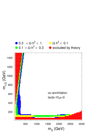
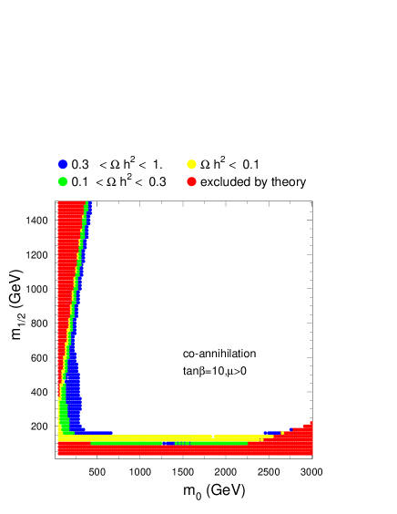
Figure 1: Regions of neutralino relic density in the $m_{0}\ vs.\ m_{1/2}$ plane for $A_{0}=0$ and $\tan\beta=10$.

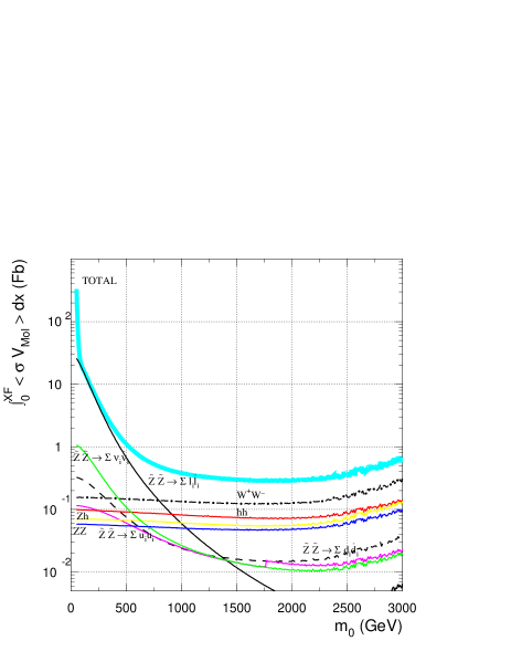
Figure 2: Thermally averaged cross section times velocity integrated from $T=0$ to $T_{F}$, for various subprocess. The thick light-grey(light-blue) curve denotes the total of all annihilation and co-annihilation reactions; $m_{1/2}=300$ GeV, $\mu>0$, $A_{0}=0$ and $\tan\beta=10$.

The dark shaded (red) regions are excluded by theoretical constraints (lack of REWSB on the right, a charged LSP in the upper left). The unshaded regions have $\Omega_{\widetilde{Z}_{1}}h^{2}>1$, and should be excluded, as they would lead to a universe of age less than 10 billion years, in conflict with the oldest stars found in globular clusters. The medium shaded (green) region yields values of $0.1<\Omega_{\widetilde{Z}_{1}}h^{2}<0.3$, i.e. in the most cosmologically favored region. The light shaded (yellow)($\Omega_{\widetilde{Z}_{1}}h^{2}<0.1$) and black(blue) ($0.3<\Omega_{\widetilde{Z}_{1}}h^{2}<1$) correspond to regions with intermediate values of low and high relic density, respectively. Points with $m_{1/2}\stackrel{{\scriptstyle<}}{{\sim}}150$ GeV give rise to chargino masses below bounds from LEP2; the LEP2 excluded regions due to chargino, slepton and Higgs searches are not shown on these plots. The structure of these plots can be understood by examining the thermally averaged cross section times velocity, integrated from zero temperature to $T_{F}$. In Fig. 2 we show this quantity for a variety of contributing subprocesses plotted versus $m_{0}$ for fixed $m_{1/2}=300$ GeV, $\mu>0$, and all other parameters as in Fig. 1. At low values of $m_{0}$, the neutralino annihilation cross section is dominated by $t$-channel scattering into leptons pairs, as shown by the black solid curve. However, at the very lowest values of $m_{0}$, the annihilation rate is sharply increased by neutralino-stau and stau-stau co-annihilations, leading to very low relic densities where $m_{\widetilde{Z}_{1}}\simeq m_{\tilde{\tau}_{1}}$[26]. As $m_{0}$ increases, the slepton masses also increase, which suppresses the annihilation cross section, and the relic density rises to values $\Omega_{\widetilde{Z}_{1}}h^{2}>1$. When $m_{0}$ increases further, to beyond the $\sim 1$ TeV level, and approaches the excluded region, the magnitude of the $\mu$ parameter falls, and the higgsino component of $\widetilde{Z}_{1}$ increases. This is the so called “focus point” region, explored in Ref. [25]. In this region, the annihilation rate is dominated by scattering into $WW$, $ZZ$, $hh$ and $Zh$ channels. At even higher $m_{0}$ values, $m_{\widetilde{Z}_{1}}\simeq m_{\widetilde{W}_{1}}\simeq m_{\widetilde{Z}_{2}}$, and these co-annihilation channels increase even more the annihilation rate. Finally, at the large $m_{0}$ bound on parameter space, $|\mu|\rightarrow 0$, and appropriate REWSB no longer occurs. Most of the structure of Fig. 1 can be understood in these terms, with the exception being the horizontal band of very low relic density at $m_{1/2}\simeq 125$ GeV. In this region, which is nearly excluded by LEP2 bounds on the chargino mass, there is enhanced neutralino annihilation through the $Z$ and $h$ resonances. In fact, a higher degree of resolution on our plots would resolve these horizontal bands into two bands, corresponding to each of the separate resonances, as shown in Ref. [20]. The $m_{0}\ vs.\ m_{1/2}$ planes for $\tan\beta=30$ are shown in Fig.3. The structure of these plots are qualitatively the same as in Fig. 1. Quantitatively, they differ mainly in that the cosmologically favored regions are expanding as $\tan\beta$ grows. One reason is that the light stau becomes even lighter as $\tan\beta$ increases, and this increases the neutralino annihilation rate $\widetilde{Z}_{1}\widetilde{Z}_{1}\rightarrow\tau\bar{\tau}$ through $t$-channel stau exchange. In addition, the bottom and tau Yukawa couplings increase with $\tan\beta$, which increases the annihilation cross sections into $\tau$s and $b$s. Finally, the $H$ and $A$ Higgs boson masses are decreasing with $\tan\beta$, and annihilation rates which proceed through these resonances increase. Co-annihilations again gives enhanced annihilation cross sections on the left and farthest right hand sides of the allowed parameter space. The glitch in contours around $m_{0}\sim 2700$ GeV and $m_{1/2}\sim 425$ GeV occurs because $m_{\widetilde{Z}_{1}}\simeq m_{t}=175$ GeV, so that $\sigma(\widetilde{Z}_{1}\widetilde{Z}_{1}\rightarrow t\bar{t})$ becomes large.

Figure 3: Regions of neutralino relic density in the $m_{0}\ vs.\ m_{1/2}$ plane for $A_{0}=0$ and $\tan\beta=30$.

Figure 4: Regions of neutralino relic density in th $m_{0}\ vs.\ m_{1/2}$ plane for $A_{0}=0$ and $\tan\beta=45$.

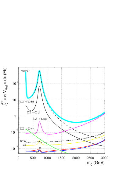
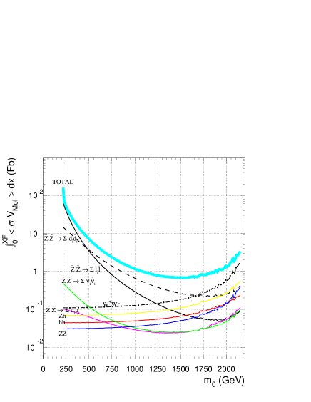
Figure 5: Thermally averaged cross section times velocity evaluated at $T_{F}$ for various subprocesses. The thick light-grey(light-blue) curve denotes the total of all annihilation and co-annihilation reactions. Left: $m_{1/2}=600$ GeV, $\mu<0$, $A_{0}=0$ and $\tan\beta=45$. Right: $m_{1/2}=300$ GeV, $\mu>0$, $A_{0}=0$ and $\tan\beta=45$.

In Fig. 4, we show the $m_{0}\ vs.\ m_{1/2}$ plane for $\tan\beta=45$. In this case, the structure of the plane is changing qualitatively, especially for $\mu<0$. First, there is a new region of disallowed parameter space for $\mu<0$ in the lower left due to $m_{A}^{2}<0$, which signals a breakdown of the REWSB mechanism. Second, a corridor of very low relic density passes diagonally through the plot. The center of this region is where $2m_{\widetilde{Z}_{1}}\simeq m_{A}$ and $m_{H}$. At the $A$ and $H$ resonance, there is very efficient neutralino annihilation into $b\bar{b}$ final states. This is illustrated in Fig. 5(left), where we show the integrated annihilation cross section times velocity versus $m_{0}$ for $m_{1/2}=600$ GeV and $\mu<0$. At the very lowest values of $m_{0}$, there is again the sharp peak due to neutralino-stau and stau-stau co-annihilations. For larger values of $m_{0}$, however, the annihilation rate is dominantly into $b\bar{b}$ final states over almost the entire $m_{0}$ range. This is due to the large annihilation rates through the $s$-channel $A$ and $H$ diagrams, even when the reactions occur off resonance. In this case, the widths of the $A$ and $H$ are so large (both $\sim 10-40$ GeV across the range in $m_{0}$ shown) that efficient $s$-channel annihilation can occur throughout considerable part of the parameter space, even when the resonance condition is not exactly fulfilled. The resonance annihilation is explicitly displayed in this plot as the annihilation bump at $m_{0}$ just below 1300 GeV. Another annihilation possibility is that $\widetilde{Z}_{1}\widetilde{Z}_{1}\rightarrow b\bar{b}$ via $t$ and $u$ channel graphs. In fact, these annihilation graphs are enhanced due to the large $b$ Yukawa coupling and decreasing value of $m_{\tilde{b}_{1}}$, but we have checked that the $s$-channel annihilation is still far the dominant channel. Annihilation into $\tau\bar{\tau}$ is the next most likely channel, but is always below the level of annihilation into $b\bar{b}$ for the parameters shown in Fig. 5(left). At even higher values of $m_{0}$ where the higgsino component of $\widetilde{Z}_{1}$ becomes non-negligible, the annihilations into $WW$ and $ZZ$ again become important; finally, at the highest values of $m_{0}$, the $\widetilde{W}_{1}$ and $\widetilde{Z}_{2}$ co-annihilation channels become large.

In Fig. 5(right), we show again the subprocess annihilation rates versus $m_{0}$ for $\tan\beta=45$, but this time for $\mu>0$ and for $m_{1/2}=300$ GeV. Although no explicit resonance is evident for $\mu>0$, the dominant annihilations are once again into $b\bar{b}$ final states over most of the parameter space, due to the wide Higgs resonances. To summarize the regions of mSUGRA model parameter space with reasonable values of neutralino relic density, we can label four important regions: $i.$) annihilation through $t$-channel slepton– especially stau– exchange, as occurs for low values of $m_{0}$ and $m_{1/2}$, $ii.$) the stau co-annihilation region for low values of $m_{0}$ on the edge of the excluded region, $iii.$) the large $m_{0}$ region with non-negligible higgsino-component annihilation, and also $\widetilde{W}_{1}$ (and possibly $\widetilde{Z}_{2}$) co-annihilation occurs near the edge of the limit of parameter space, and $iv.$) annihilation into $b\bar{b}$ and $\tau\bar{\tau}$ final states through $s$-channel $A$ and $H$ resonances at high $\tan\beta$. Other regions can include top or bottom squark co-annihilation for large values of $A_{0}$, again on the edge of parameter space where $\tilde{t}_{1}$ or $\tilde{b}_{1}$ become light, or annihilation through $Z$ or $h$ resonances. The $Z-$resonance region is essentially excluded now by constraints on sparticle masses from LEP2.

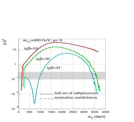
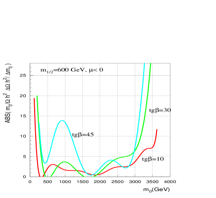
Figure 6: Neutralino relic density $\Omega_{\widetilde{Z}_{1}}h^{2}$(left) and the fine tuning parameter(right)[defined by Eq.(8)], versus $m_{0}$ for $A_{0}=0$, $m_{1/2}=600$ GeV, $\mu<0$ and $\tan\beta=10$, 30 and 45.

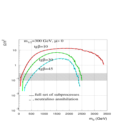
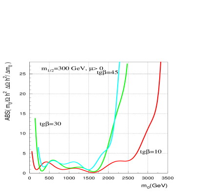
Figure 7: The same as Fig. 6 but for $m_{1/2}=600$ GeV and $\mu<0$.

It is useful to view the relic density $\Omega_{\widetilde{Z}_{1}}h^{2}$ directly as a function of model parameters. We show in Fig. 6(left) the value of $\Omega_{\widetilde{Z}_{1}}h^{2}$ versus the parameter $m_{0}$ for fixed $m_{1/2}=600$ GeV, $A_{0}=0$, $\mu<0$ and for $\tan\beta=10$, 30 and 45. The dashed curves show the result with no co-annihilations, while the solid curves yield the complete calculation. The shaded band denotes the cosmologically favored region with $0.1<\Omega_{\widetilde{Z}_{1}}h^{2}<0.3$. For this value of $m_{1/2}$, the lower $\tan\beta$ curves yield a favored relic density only in the very low and very high $m_{0}$ regions, and here the curves have a very sharp slope. The large slope is indicative of large fine-tuning, in that a small change of model parameters, in this case $m_{0}$, yields a large change in $\Omega_{\widetilde{Z}_{1}}h^{2}$. In contrast, the $\tan\beta=45$ curve shows a large region with good relic density and nearly zero slope($\mu>0$) or not very steep slope($\mu<0$), and hence with little fine-tuning. In Fig. 6(right), we show the corresponding values of the fine-tuning, basically the logarithmic derivative, as advocated by Ellis and Olive[37]:

$$\Delta(m_{0})=\left|\frac{m_{0}}{\Omega_{\widetilde{Z}_{1}}h^{2}}\frac{\partial\Omega_{\widetilde{Z}_{1}}h^{2}}{\partial m_{0}}\right|$$ (8)

As indicated earlier, the low fine-tuning regions mostly coincide with that of neutralino annihilation via $t$-channel slepton exchange (region $i.$)), or off-resonance annihilation through $A$ and $H$ (region $iv.$)). The co-annihilation region $ii.)$ and focus point region $iii.$) tend to have higher fine-tunings due to the steep rise of the cross sections. Regions with simultaneous low fine- tuning and preferred $\Omega_{\widetilde{Z}_{1}}h^{2}$ values are the best candidates for viable mSUGRA parameters. In Fig. 7(left), we show $\Omega_{\widetilde{Z}_{1}}h^{2}$ versus $m_{0}$ for $m_{1/2}=300$ GeV, $A_{0}=0$, $\mu>0$ and the same three $\tan\beta$ parameters. The curves reflect the broad regions of parameter space with reasonable relic density values at high $\tan\beta$. The corresponding plot of the fine-tuning parameter is shown in Fig. 7(right). Again, there is large fine-tuning at the edges of parameter space, but low fine-tuning in the intermediate regions. In conclusion, the relic density and the fine-tuning parameter together tend to prefer mSUGRA model parameters in regions $i.$) or $iv.$). These two regions lead to distinct collider signatures for future searches for supersymmetric matter.

4 Conclusions

In conclusion, we have performed a calculation of the neutralino relic density in the minimal supergravity model including all $2\rightarrow 2$ neutralino annihilation and co-annihilation processes, where the initial state includes $\widetilde{Z}_{1}$, $\widetilde{Z}_{2}$, $\widetilde{W}_{1}$, $\tilde{e}_{1}$, $\tilde{\mu}_{1}$, $\tilde{\tau}_{1}$, $\tilde{t}_{1}$ and $\tilde{b}_{1}$. The calculation was performed using the CompHEP program for automatic evaluation of Feynman diagrams, coupled with ISAJET for sparticle mass evaluation in the mSUGRA model, and for standard and supersymmetric couplings and decay widths. We implemented relativistic thermal averaging, which is especially important for evaluating the relic density when resonances in the annihilation cross section are present, and neutralino thermal velocities can be relativistic. The three-dimensional integration was performed by Monte Carlo evaluation with importance sampling, which yields in general good convergence even in the presence of narrow resonances. We note that a calculation of similar scope and procedure was recently reported in Ref. [34].

We found four regions of parameter space that led to relic densities in accord with results from cosmological measurements, i.e. $0.1<\Omega_{\widetilde{Z}_{1}}h^{2}<0.3$. These include i.) the region dominated by $t$-channel slepton exchange, ii.) the region dominated by stau co-annihilation, iii.) the large $m_{0}$ region dominated by a more higgsino-like neutralino and iv.) the broad regions at high $\tan\beta$ dominated by off-shell annihilation through the $A$ and $H$ Higgs boson resonances. Regions ii.) and iii.) generally have large fine-tuning associated with them, and although it is logically possible that nature has chosen such parameters, any slight deviation of model parameters would lead to either too low or too high a relic density. Region i.) generally has the property that some of the sleptons have masses less than about 300-400 GeV. This region can give rise to a rich set of collider signatures, since many of the sparticles are relatively light.

Region iv.) gives broad regions of model parameter space with reasonable values of relic density as well as low values of the fine-tuning parameter. It can also allow quite heavy values of SUSY particle masses, which would be useful to suppress many flavor-violating (such as $b\rightarrow s\gamma$)[44] and CP violating loop processes, and the muon $g-2$ value[45]. In many respects region iv.) is a favored region of parameter space. The neutralino relic density may well point the way to the sort of SUSY signatures we should expect at high energy collider experiments.

We thank Manuel Drees, Konstantin Matchev, Leszek Roszkowski and Xerxes Tata for discussions. This research was supported in part by the U.S. Department of Energy under contract number DE-FG02-97ER41022.

References

- [1] A. T. Lee et al. (MAXIMA Collaboration), Astrophys. J. 561, L1 (2001); C. B. Netterfield et al. (BOOMERANG Collaboration), astro-ph/0104460 (2001); N. W. Halverson et al. (DASI Collaboration), astro-ph/0104489 (2001); P. de Bernardis et al., astro-ph/0105296 (2001).
- [2] See e.g. W. L. Freedman, Phys. Rept. 333, 13 (2000).
- [3] A. G. Riess et al., Astron. J. 116, 1009 (1998); S. Perlmutter et al., Astrophys. J. 517, 565 (1999).
- [4] A. H. Jaffe et al., Phys. Rev. Lett. 86, 3475 (2001).
- [5] K. Olive, G. Steigman and T. Walker, Phys. Rept 333-334, 389 (2000); S. Burles, K. Nollet and M. Turner, Phys. Rev. Lett. 82, 4176 (1999) and Phys. Rev. D63, 063512 (2001); D. Tytler, J. O’Meara, N. Suzuki and D. Lubin, astro-ph/0001318 (2000).
- [6] For a review, see e.g. M. S. Turner, astro-ph/0108103 (2001).
- [7] For a review, see G. Jungman, M. Kamionkowski and K. Griest, Phys. Rept. 267, 195 (1996).
- [8] A. Chamseddine, R. Arnowitt and P. Nath, Phys. Rev. Lett. 49, 970 (1982); R. Barbieri, S. Ferrara and C. Savoy, Phys. Lett. B119, 343 (1982); L.J. Hall, J. Lykken and S. Weinberg, Phys. Rev. D27, 2359 (1983).
- [9] H. Baer, F. Paige, S. Protopopescu and X. Tata, hep-ph/0001086 (2000).
- [10] H. Goldberg, Phys. Rev. Lett. 50, 1419 (1983); J. Ellis, J. Hagelin, D. Nanopoulos and M. Srednicki, Phys. Lett. B127, 233 (1983); J. Ellis, J. Hagelin, D. Nanopoulos, K. Olive and M. Srednicki, Nucl. Phys. B238, 453 (1984).
- [11] M. Srednicki, R. Watkins and K. Olive, Nucl. Phys. B310, 693 (1988).
- [12] R. Barbieri, M. Frigeni and G. F. Giudice, Nucl. Phys. B313, 725 (1989);
- [13] K. Griest, M. Kamionkowski and M. Turner, Phys. Rev. D41, 3565 (1990).
- [14] K. Griest and D. Seckel, Phys. Rev. D43, 3191 (1991).
- [15] P. Gondolo and G. Gelmini, Nucl. Phys. B360, 145 (1991).
- [16] A. Bottino, V. de Alfaro, N. Fornengo, G. Mignola and S. Scopel, Astropart. Phys. 1, 61 (1992); A. Bottino et al., Astropart. Phys. 2, 67 (1994); V. Berezinsky et al., Astropart. Phys. 5, 1 (1996).
- [17] M. Drees and M. Nojiri, Phys. Rev. D47, 376 (1993).
- [18] J. Ellis and L. Roszkowski, Phys. Lett. B283, 252 (1992); L. Roszkowski and R. Roberts, Phys. Lett. B309, 329 (1993); G. Kane, C. Kolda, L. Roszkowski and J. Wells, Phys. Rev. D49, 6173 (1994).
- [19] P. Nath and R. Arnowitt, Phys. Rev. Lett. 70, 3696 (1993); R. Arnowitt and P. Nath, Phys. Lett. B437, 344 (1998).
- [20] H. Baer and M. Brhlik, Phys. Rev. D53, 597 (1996) and Phys. Rev. D57, 567 (1998); H. Baer, M. Brhlik, M. A. Diaz, J. Ferrandis, P. Mercadante, P. Quintana and X. Tata, Phys. Rev. D 63, 015007 (2001)
- [21] J. Edsjö and P. Gondolo, Phys. Rev. D56, 1879 (1997).
- [22] V. Barger and C. Kao, Phys. Rev. D57, 3131 (1998) and Phys. Lett. B518, 117 (2001).
- [23] J. Ellis, T. Falk, G. Ganis, K. Olive and M. Srednicki, Phys. Lett. B510, 236 (2001).
- [24] DarkSUSY, by P. Gondolo and J. Edsjö, astro-ph/0012234 (2000).
- [25] J. Feng, K. Matchev and F. Wilczek, Phys. Lett. B482, 388 (2000) and Phys. Rev. D63, 045024 (2001); see also hep-ph/0111295 (2001).
- [26] J. Ellis, T. Falk and K. Olive, Phys. Lett. B444, 367 (1998); J. Ellis, T. Falk, K. Olive and M. Srednicki, Astropart. Phys. 13, 181 (2000).
- [27] R. Arnowitt, B. Dutta and Y. Santoso, Nucl. Phys. B606, 59 (2001).
- [28] M. Gomez, G. Lazarides and C. Pallis, Phys. Rev. D61, 123512 (2000) and Phys. Lett. B487, 313 (2000).
- [29] L. Roszkowski, R. Ruiz de Austri and T. Nihei, JHEP0108, 024 (2001).
- [30] A. Djouadi, M. Drees and J. Kneur, JHEP0108, 055 (2001).
- [31] C. Boehm, A. Djouadi and M. Drees, Phys. Rev. D62, 035012 (2000).
- [32] J. Ellis, K. Olive and Y. Santoso, hep-ph/0112113 (2001).
- [33] CompHEP v.33.23, by A. Pukhov et al., hep-ph/9908288 (1999).
- [34] G. Belanger, F. Boudjema, A. Pukhov and A. Semenov, hep-ph/0112278 (2001).
- [35] T. Nihei, L. Roszkowski and R. R. de Austri, hep-ph/0202009 (2002).
- [36] S. Kawabata, Prepared for 2nd International Workshop on Software Engineering, Artificial Intelligence and Expert Systems for High-energy and Nuclear Physics, La Londe Les Maures, France, 13-18 Jan 1992.
- [37] J. Ellis and K. Olive, Phys. Lett. B514, 114 (2001).
- [38] See e.g. R. Barate et al., Phys. Lett. B499, 67 (2001).
- [39] For combined LEP2 limits on MSSM Higgs bosons, see hep-ex/0107030 (2001).
- [40] H. Baer, M. Drees, F. Paige, P. Quintana and X. Tata, Phys. Rev. D61, 095007 (2000); V. Barger and C. Kao, Phys. Rev. D60, 115015 (1999); K. Matchev and D. Pierce, Phys. Lett. B467, 225 (1999); for a review, see S. Abel et al., hep-ph/0003154 (2000).
- [41] J. Feng, K. Matchev and T. Moroi, Phys. Rev. D61, 075005 (2000).
- [42] H. Baer, C. H. Chen, F. Paige and X. Tata, Phys. Rev. D52, 2746 (1995) and Phys. Rev. D53, 6241 (1996); H. Baer, C. H. Chen, M. Drees, F. Paige and X. Tata, Phys. Rev. D59, 055014 (1999).
- [43] H. Baer, R. Munroe and X. Tata, Phys. Rev. D54, 6735 (1996); Erratum Phys. Rev. D56, 4424 (1997).
- [44] See e.g. H. Baer, M. Brhlik, D. Castano and X. Tata, Phys. Rev. D58, 015007 (1998).
- [45] See e.g. H. Baer, C. Balazs, J. Ferrandis and X. Tata, Phys. Rev. D64, 035004 (2001).