Abstract

In the Minimal Supersymmetric Standard Model (MSSM) we calculate the corrections to neutral ${\cal CP}$-even Higgs-boson production in the $WW$-fusion and Higgs-strahlung channel, $e^{+}e^{-}\to\bar{\nu}\nu\,\{h,H\}$, at a future Linear Collider, taking into account all ${\cal O}(\alpha)$ corrections arising from loops of fermions and sfermions. For the production of the lightest MSSM Higgs boson, $h$, we find genuine loop corrections (beyond the universal Higgs propagator corrections) of up to $-5\%$. For the heavy ${\cal CP}$-even neutral Higgs boson, $H$, which shows decoupling behavior at tree level, we find non-negligible corrections that can enhance the cross section considerably in parts of the MSSM parameter space. At a center-of-mass energy of $\sqrt{s}=1000\,\,\mathrm{GeV}$, heavy ${\cal CP}$-even Higgs-boson masses of up to $M_{H}\lesssim 700\,\,\mathrm{GeV}$ are accessible at the Linear Collider in favorable regions of the MSSM parameter space.

1 Introduction

Disentangling the origin of electroweak symmetry breaking is one of the main tasks of the current and next generation of colliders. The prime candidate is a Higgs mechanism with elementary scalar particles below the TeV scale. Within the electroweak Standard Model (SM) the minimal version of the Higgs mechanism is implemented, i.e. one doublet of complex scalar fields giving rise to one physical Higgs boson. On the other hand, theories based on Supersymmetry (SUSY) [1] are widely considered as the theoretically most appealing extension of the SM. Contrary to the SM, two Higgs doublets are required in the minimal realization, resulting in five physical Higgs bosons [2]. The Higgs sector of the Minimal Supersymmetric Standard Model (MSSM) can be expressed at lowest order in terms of $M_{Z}$, $M_{A}$ (the mass of the ${\cal CP}$-odd Higgs boson), and $\tan\beta=v_{2}/v_{1}$, the ratio of the two vacuum expectation values. While the discovery of one light Higgs boson might well be compatible with the predictions both of the SM and the MSSM, the discovery of one or more other heavy Higgs boson would be a clear and unambiguous signal for physics beyond the SM.

In the decoupling limit, i.e. for $M_{A}\gtrsim 200\,\,\mathrm{GeV}$, the heavy MSSM Higgs bosons are nearly degenerate in mass, $M_{A}\sim M_{H}\sim M_{H^{\pm}}$. The couplings of the neutral Higgs bosons to SM gauge bosons are proportional to

$$\begin{gathered}VVh\sim VHA\sim\sin(\beta-\alpha)\,,\\ VVH\sim VhA\sim\cos(\beta-\alpha)\,,\end{gathered}\qquad(V=Z,W^{\pm})$$ (1)

where $\alpha$ is the angle that diagonalizes the ${\cal CP}$-even Higgs sector. In the decoupling limit one finds $\beta-\alpha\to\pi/2$, i.e. $\sin(\beta-\alpha)\to 1$, $\cos(\beta-\alpha)\to 0$.

At the LC, the possible channels for neutral Higgs-boson production are the production via $Z$-boson exchange,

$$e^{+}e^{-} \to Z^{*}\to Z\{h,H\}\,,$$ (2)

$$e^{+}e^{-} \to Z^{*}\to A\{h,H\}\,,$$

and the $WW$-fusion channel,

$$e^{+}e^{-}\to\bar{\nu}_{e}W^{+}\;\nu_{e}W^{-}\to\bar{\nu}_{e}\nu_{e}\{h,H\}\,.$$ (3)

As a consequence of the coupling structure, in the decoupling limit the heavy Higgs boson can only be produced in $(H,A)$ pairs. This limits the LC reach to $M_{H}\lesssim\sqrt{s}/2$. Higher-order corrections to the $WW\to H$ channel from loops of fermions and sfermions, however, involve potentially large contributions from the top and bottom Yukawa couplings and could thus significantly affect the decoupling behavior.

In this paper we have evaluated the one-loop corrections of fermions and sfermions to the process $e^{+}e^{-}\to\bar{\nu}\nu\,\{h,H\}$, i.e. to the production of a neutral ${\cal CP}$-even Higgs boson in association with a neutrino pair both via the $WW$-fusion and the Higgs-strahlung mechanism. In the latter case the $Z$ boson is connected to a neutrino pair, $e^{+}e^{-}\to Z\{h,H\}\to\bar{\nu}_{l}\nu_{l}\{h,H\}$, with $l=e,\mu,\tau$ (where the latter two neutrinos result in an indistinguishable final state in the detector). Our results have been derived using the packages FeynArts, FormCalc, and LoopTools [3, 4].

While the well-known universal Higgs-boson propagator corrections turned out not to significantly modify the decoupling behavior of the heavy ${\cal CP}$-even Higgs boson, an analysis of the process-specific contributions to the $WWH$ vertex has been missing so far. Taking into account all loop and counter-term contributions to the process $e^{+}e^{-}\to\bar{\nu}\nu\,\{h,H\}$ from fermions and sfermions and including also the effects of beam polarization in our analysis, we investigate in this paper the LC reach for the heavy ${\cal CP}$-even Higgs boson. We have obtained results for values of the MSSM parameters according to the four benchmark scenarios defined in Ref. [5]. While within these benchmark scenarios we find that the loop corrections do not significantly enhance the LC reach for heavy ${\cal CP}$-even Higgs boson production and in some cases even slightly reduce the accessible parameter space, we have also investigated MSSM parameter regions where the loop effects do in fact lead to a significant improvement of the LC reach. In “favorable” MSSM parameter regions an $e^{+}e^{-}$ LC running at $\sqrt{s}=1$ TeV can be capable of producing a heavy ${\cal CP}$-even Higgs boson with a mass up to $M_{H}\lesssim 700$ GeV.

Concerning the production of the light ${\cal CP}$-even Higgs boson, an accurate prediction of the production cross section for precision analyses will be necessary. Aiming for analyses at the percent level [6] also requires a prediction of the production cross section in this range of precision. Besides the already known universal Higgs propagator corrections, in particular loops from fermions and sfermions (especially from the third family) are expected to give relevant contributions. We analyze our results for the parameters of the four benchmark scenarios defined in Ref. [5] and study the results as a function of different SUSY parameters. We discuss the relative importance of the fermion- and the sfermion-loop contributions and furthermore evaluate the fermion-loop correction within the SM for comparison purposes.

Electroweak loop effects on processes within the MSSM where a single Higgs boson is produced have recently drawn considerable interest in the literature, and we compare our results to existing ones where there is overlap. Within the SM, the tree-level results for Higgs-boson production in the $WW$-fusion channel are available for several years already [7, 8]. On the other hand, evaluating the full one-loop corrections within the SM has been attempted only very recently [9]. In the MSSM, corrections from third-generation fermions and sfermions to $e^{+}e^{-}\to\bar{\nu}\nu\,h$ have been presented in Ref. [10]. Production of the heavy ${\cal CP}$-even Higgs boson has only been considered in Ref. [10] for small values of $M_{A}$, where the heavy ${\cal CP}$-even Higgs boson has SM-like couplings, while the decoupling region has not been investigated. We have compared our results for the production of the light ${\cal CP}$-even Higgs boson (restricted to the corrections from the third generation only) with the ones given in Ref. [10] and find significant deviations. While the authors of Ref. [10] find large corrections from the loops of third generation fermions both in the SM and in the MSSM, the correction from this class of diagrams in our result turns out to be much smaller and does not exceed $\pm 2$%.

Electroweak loop effects have also been evaluated for other processes with single Higgs-boson production within the MSSM. The process $e^{+}e^{-}\to\nu_{e}\bar{\nu}_{e}A$ has been evaluated at the full one-loop level in Ref. [11], where the cross section has been found to be too small for $A$ detection at the LC via this channel. The results for the Higgs-strahlung process, $e^{+}e^{-}\to Z^{*}\to Z\{h,H\}$, and the associated production, $e^{+}e^{-}\to Z^{*}\to A\{h,H\}$, containing the complete one-loop contributions and the leading two-loop corrections entering via Higgs-boson propagators, have been given in Ref. [12]. The two-loop corrections have been found to yield corrections at the 5–10% level. As explained above, these processes are not suitable for heavy Higgs boson production with $M_{A}>\sqrt{s}/2$. Furthermore, the production of a charged Higgs boson in association with a $W$ boson has been evaluated, including the full one-loop corrections [13, 14]. It has been found that this channel possesses only a small potential for charged Higgs boson production with $M_{H^{\pm}}>\sqrt{s}/2$.

The rest of the paper is organized as follows: In Sect. 2 we review the necessary features of the MSSM Higgs sector. Details about the calculation are presented in Sect. 3. The numerical analysis for light and heavy ${\cal CP}$-even Higgs boson production, the corresponding SM result, and the comparison with existing results can be found in Sect. 4. We conclude with Sect. 5.

2 The MSSM Higgs sector

At the tree level the mass matrix of the neutral ${\cal CP}$-even Higgs bosons in the $\phi_{1},\phi_{2}$ basis can be expressed in terms of $M_{Z}$, $M_{A}$ (the mass of the ${\cal CP}$-odd Higgs boson), and $\tan\beta=v_{2}/v_{1}$, the ratio of the two vacuum expectation values, as follows [2]:

$$M_{\rm Higgs}^{2,{\rm tree}} =\begin{pmatrix}m_{\phi_{1}}^{2}&m_{\phi_{1}\phi_{2}}^{2}\\ m_{\phi_{1}\phi_{2}}^{2}&m_{\phi_{2}}^{2}\end{pmatrix}$$

$$=\begin{pmatrix}M_{A}^{2}\sin^{2}\beta\hskip 2.84526pt+M_{Z}^{2}\cos^{2}\beta\hskip 2.84526pt&-(M_{A}^{2}+M_{Z}^{2})\sin\beta\hskip 2.84526pt\cos\beta\hskip 2.84526pt\\ -(M_{A}^{2}+M_{Z}^{2})\sin\beta\hskip 2.84526pt\cos\beta\hskip 2.84526pt&M_{A}^{2}\cos^{2}\beta\hskip 2.84526pt+M_{Z}^{2}\sin^{2}\beta\hskip 2.84526pt\end{pmatrix}.$$ (4)

Transforming to the mass-eigenstate basis yields

$$M_{\rm Higgs}^{2,{\rm tree}}\overset{\alpha}{\longrightarrow}\left(\begin{array}[]{cc}m_{H}^{2}&0\\ 0&m_{h}^{2}\end{array}\right),$$ (5)

$m_{h}$ and $m_{H}$ being the tree-level masses of the neutral ${\cal CP}$-even Higgs bosons and

$$\begin{pmatrix}H\\ h\end{pmatrix} =\begin{pmatrix}\cos\alpha\hskip 2.84526pt&\sin\alpha\hskip 2.84526pt\\ -\sin\alpha\hskip 2.84526pt&\cos\alpha\hskip 2.84526pt\end{pmatrix}\begin{pmatrix}\phi_{1}\\ \phi_{2}\end{pmatrix}.$$ (6)

The mixing angle $\alpha$ is related to $\tan\beta$ and $M_{A}$ by

$$\tan 2\alpha=\tan 2\beta\,\frac{M_{A}^{2}+M_{Z}^{2}}{M_{A}^{2}-M_{Z}^{2}}\,,\quad-\frac{\pi}{2}<\alpha<0\,.$$ (7)

In the Feynman-diagrammatic approach, the higher-order-corrected masses of the two ${\cal CP}$-even Higgs bosons, $M_{h}$ and $M_{H}$, are derived beyond tree level by determining the poles of the $h$–$H$-propagator matrix whose inverse is given by

$$\left(\Delta_{\rm Higgs}\right)^{-1}=-\mathrm{i}\begin{pmatrix}q^{2}-m_{H}^{2}+\hat{\Sigma}_{H}(q^{2})&\hat{\Sigma}_{hH}(q^{2})\\ \hat{\Sigma}_{hH}(q^{2})&q^{2}-m_{h}^{2}+\hat{\Sigma}_{h}(q^{2})\end{pmatrix},$$ (8)

where the $\hat{\Sigma}$ denote the renormalized Higgs-boson self-energies. Determining the poles of the matrix $\Delta_{\rm Higgs}$ in Eq. (8) is equivalent to solving the equation

$$\left[q^{2}-m_{h}^{2}+\hat{\Sigma}_{hh}(q^{2})\right]\left[q^{2}-m_{H}^{2}+\hat{\Sigma}_{HH}(q^{2})\right]-\left[\hat{\Sigma}_{hH}(q^{2})\right]^{2}=0\,.$$ (9)

The renormalized Higgs-boson self-energies are given by

$$\hat{\Sigma}_{HH}(q^{2}) =\Sigma_{HH}(q^{2})+\delta Z_{H}(q^{2}-m_{H}^{2})-\delta m_{H}^{2}\,,$$ (10)

$$\hat{\Sigma}_{hH}(q^{2}) =\Sigma_{hH}(q^{2})+\frac{1}{2}\delta Z_{Hh}(q^{2}-m_{H}^{2})+\frac{1}{2}\delta Z_{hH}(q^{2}-m_{h}^{2})-\delta m_{hH}^{2}\,,$$

$$\hat{\Sigma}_{hh}(q^{2}) =\Sigma_{hh}(q^{2})+\delta Z_{h}(q^{2}-m_{h}^{2})-\delta m_{h}^{2}\,.$$

The mass counter terms arise from the renormalization of the Higgs potential, see Ref. [15]. They are evaluated in the on-shell renormalization scheme. The field-renormalization constants can be obtained in the $\overline{\rm{MS}}$ scheme, leading to

$$\delta Z_{H} =-\left[\mathop{\rm Re}\Sigma_{HH}^{\prime}(m_{H}^{2})\right]^{\rm div},$$ (11)

$$\delta Z_{h} =-\left[\mathop{\rm Re}\Sigma_{hh}^{\prime}(m_{h}^{2})\right]^{\rm div},$$

$$\delta Z_{hH} =\frac{\sin\alpha\hskip 2.84526pt\cos\alpha\hskip 2.84526pt}{\cos 2\alpha\hskip 2.84526pt}(\delta Z_{h}-\delta Z_{H})\,,$$

$$\delta Z_{Hh} =\delta Z_{hH}\,,$$

i.e. only the divergent parts of the renormalization constants in Eqs. (11) are taken into account. As renormalization scale we have chosen $\mu^{\overline{\rm{MS}}}=m_{t}$.

3 The process $e^{+}e^{-}\to\bar{\nu}_{e}\nu_{e}\,\{h,H\}$

3.1 The tree-level process

The tree-level process [7, 8] consists of the two diagrams shown in Fig. 1. Besides the $WW$-fusion contribution (left diagram), we also take into account the Higgs-strahlung contribution (right diagram), where a virtual $Z$ boson is connected to two electron neutrinos.

Figure 1: The tree-level diagrams for the process $e^{+}e^{-}\to\bar{\nu}\nu\,\{h,H\}$, consisting of the $WW$-fusion contribution (left) and the Higgs-strahlung contribution (right).

An analytical expression for the tree-level cross section for an SM Higgs boson can be found e.g. in Ref. [17]. For relatively low energies and moderate values of the SM Higgs-boson mass ($\sqrt{s}\lesssim 400\,\,\mathrm{GeV}$, $M_{H_{\rm SM}}\lesssim 200\,\,\mathrm{GeV}$) the resonant production via the Higgs-strahlung contribution dominates over the $WW$-fusion contribution. At higher energies, however, the $WW$-fusion contribution becomes dominant. The cross section, containing both contributions, in the high-energy limit takes the simple form [8]

$$\sigma(e^{+}e^{-}\to\bar{\nu}_{e}\nu_{e}H_{\rm SM})\to\frac{G_{F}^{3}M_{W}^{4}}{4\sqrt{2}\,\pi^{3}}\left[\left(1+\frac{M_{H_{\rm SM}}^{2}}{s}\right)\log\left(\frac{s}{M_{H_{\rm SM}}^{2}}\right)-2\left(1-\frac{M_{H_{\rm SM}}^{2}}{s}\right)\right],$$ (12)

where the $t$-channel contribution from the $WW$-fusion diagram gives rise to the logarithmic increase. For our numerical results we use the full MSSM tree-level matrix element, see Sect. 3.4.

The coefficients for the couplings $WWh$ and $WWH$ are denoted by $\Gamma_{h}^{(0)}$ and $\Gamma_{H}^{(0)}$ at the tree level, respectively (and analogously for the $ZZh$ and $ZZH$ couplings):

$$\Gamma_{h}^{(0)} =\frac{\mathrm{i}\,e\,M_{W}}{s_{W}}\sin(\beta-\alpha)\,,$$ (13)

$$\Gamma_{H}^{(0)} =\frac{\mathrm{i}\,e\,M_{W}}{s_{W}}\cos(\beta-\alpha)\,.$$ (14)

The SM coupling $\Gamma^{(0)}_{H_{\rm SM}}$ is obtained by dropping the SUSY factors $\sin(\beta-\alpha)$ or $\cos(\beta-\alpha)$. In the decoupling limit, $M_{A}\gtrsim 200\,\,\mathrm{GeV}$, $\beta-\alpha\to\pi/2$, so that $\sin(\beta-\alpha)\to 1$ and $\cos(\beta-\alpha)\to 0$, i.e. the heavy neutral ${\cal CP}$-even Higgs boson decouples from the $W$ and $Z$ bosons.

We parametrize the Born matrix element by the Fermi constant, $G_{F}$, i.e. we use the relation

$$e=2\;s_{W}\;M_{W}\left[\frac{\sqrt{2}\,G_{F}}{1+\Delta r}\right]^{1/2},$$ (15)

where $\Delta r$ incorporates higher-order corrections, see Sect. 3.2.

3.2 Higher-order corrections

In the description of our calculation below we will mainly concentrate on the $WW$-fusion contribution. The Higgs-strahlung contribution, which we describe in less detail, is taken into account in exactly the same way (see, however, Sect. 3.4).

We evaluate the one-loop ${\cal O}(\alpha)$ contributions from loops involving all fermions and sfermions. Especially the corrections involving third-generation fermions and sfermions, i.e. $t,b,\tau,\nu_{\tau}$, and their corresponding superpartners, $\tilde{t}_{1},\tilde{t}_{2}$, $\tilde{b}_{1},\tilde{b}_{2}$, $\tilde{\tau}_{1},\tilde{\tau}_{2}$, $\tilde{\nu}_{\tau}$, are expected to be sizable, since they contain potentially large Yukawa couplings, $y_{t}$, $y_{b}$, $y_{\tau}$, where the down-type couplings can be enhanced in the MSSM for large values of $\tan\beta$. This class of diagrams in particular contains contributions enhanced by $m_{t}^{2}/M_{W}^{2}$.

The contributions involve corrections to the $WW\{h,H\}$ vertex and the corresponding counter-term diagram, shown in Fig. 2, corrections to the $W$-boson propagators and the corresponding counter terms, shown in Fig. 3, and the counter-term contributions to the $e\nu_{e}W$ vertex as shown in Fig. 4. Furthermore, Higgs propagator corrections enter via the wave-function normalization of the external Higgs boson, see Sect. 3.3 below. There are also $W$-boson propagator corrections inducing a transition from the $W^{\pm}$ to either $G^{\pm}$ or $H^{\pm}$. These corrections affect only the longitudinal part of the $W$ boson, however, and are thus $\propto m_{e}/M_{W}$ and have been neglected.

Figure 2: Corrections to the $WW\{h,H\}$ vertex and the corresponding counter-term diagram. The label $\hbox to0.0pt{\raise 7.22223pt\hbox{\tiny${}_{\,(\;\,)}$}\hss}\tilde{f}$ denotes all (s)fermions, except in the presence of a $\hbox to0.0pt{\raise 7.22223pt\hbox{\tiny${}_{\,(\;\,)}$}\hss}\tilde{f}\,^{\prime}$, in which case the former denotes only the isospin-up and the latter the isospin-down members of the (s)fermion doublets.

Figure 3: Corrections to the $W$-boson propagator and the corresponding counter-term diagrams. The label $\hbox to0.0pt{\raise 7.22223pt\hbox{\tiny${}_{\,(\;\,)}$}\hss}\tilde{f}$ denotes all (s)fermions, except in the presence of a $\hbox to0.0pt{\raise 7.22223pt\hbox{\tiny${}_{\,(\;\,)}$}\hss}\tilde{f}\,^{\prime}$, in which case the former denotes only the isospin-up and the latter the isospin-down members of the (s)fermion doublets.

Figure 4: Counter-term contributions entering via the $e\,\nu_{e}\,W$ vertex.

While the renormalization in the counter terms depicted in Figs. 3 and 4 is as in the SM (see e.g. Ref. [18]), the $WW\{h,H\}$ vertices are renormalized as follows,

$$WWh:\quad\Gamma_{WWh}^{(0),{\rm CT}}=\Gamma_{h}^{(0)} \Biggl{[}1+\delta\tilde{Z}_{e}+\frac{1}{2}\frac{\delta M_{W}^{2}}{M_{W}^{2}}+\delta Z_{W}+\frac{\delta s_{W}}{s_{W}}$$

$${}+\sin\beta\hskip 2.84526pt\cos\beta\hskip 2.84526pt\frac{\cos(\beta-\alpha)}{\sin(\beta-\alpha)}\delta\tan\beta+\frac{1}{2}\delta Z_{h}+\frac{1}{2}\frac{\Gamma_{H}^{(0)}}{\Gamma_{h}^{(0)}}\delta Z_{Hh}\Biggr{]}\,,$$ (16)

$$WWH:\quad\Gamma_{WWH}^{(0),{\rm CT}}=\Gamma_{H}^{(0)} \Biggl{[}1+\delta\tilde{Z}_{e}+\frac{1}{2}\frac{\delta M_{W}^{2}}{M_{W}^{2}}+\delta Z_{W}+\frac{\delta s_{W}}{s_{W}}$$

$${}-\sin\beta\hskip 2.84526pt\cos\beta\hskip 2.84526pt\frac{\sin(\beta-\alpha)}{\cos(\beta-\alpha)}\delta\tan\beta+\frac{1}{2}\delta Z_{H}+\frac{1}{2}\frac{\Gamma_{h}^{(0)}}{\Gamma_{H}^{(0)}}\delta Z_{hH}\Biggr{]}\,.$$ (17)

Analogous expressions are obtained for $\Gamma_{ZZ\Phi}^{(0),{\rm CT}}$ ($\Phi=h,H$). In the above expressions $\delta\tilde{Z}_{e}$ incorporates the charge renormalization and the $\Delta r$ contribution arising from Eq. (15),

$$\delta\tilde{Z}_{e}=\delta Z_{e}-\frac{1}{2}\Delta r,\quad\delta Z_{e}=\frac{1}{2}\Pi^{\gamma}(0)-\frac{s_{W}}{c_{W}}\frac{\Sigma_{\gamma Z}^{T}(0)}{M_{Z}^{2}}\,,$$ (18)

where $\Sigma^{T}$ denotes the transverse part of a self-energy. $\delta M_{W}^{2}$ is the $W$-mass counter term, $\delta Z_{W}$ is the corresponding field-renormalization constant, and $\delta s_{W}$ denotes the renormalization constant for the weak mixing angle. The field-renormalization constants, $\delta Z_{H},\delta Z_{h}$, and $\delta Z_{Hh}=\delta Z_{hH}$ are given in Eq. (11). The counter term for $\tan\beta$ (with $\tan\beta\to\tan\beta(1+\delta\tan\beta)$) is derived in the $\overline{\rm{MS}}$ renormalization scheme [15] (using DRED). The parameter $\tan\beta$ in our result thus corresponds to the $\overline{\rm{MS}}$ parameter, taken at the scale $\mu^{\overline{\rm{MS}}}=m_{t}$. We list here all contributing counter terms except for the Higgs field renormalization which has already been given in Eq. (11):

$$\delta M_{W}^{2} =\mathop{\rm Re}\Sigma_{W}^{T}(M_{W}^{2})\,,$$ (19)

$$\delta M_{Z}^{2} =\mathop{\rm Re}\Sigma_{Z}^{T}(M_{Z}^{2})\,,$$

$$\frac{\delta s_{W}}{s_{W}} =\frac{1}{2}\frac{c_{W}^{2}}{s_{W}^{2}}\left(\frac{\delta M_{Z}^{2}}{M_{Z}^{2}}-\frac{\delta M_{W}^{2}}{M_{W}^{2}}\right),$$

$$\delta\tan\beta =\delta\tan\beta^{\overline{\rm{MS}}}=-\frac{1}{2\cos 2\alpha\hskip 2.84526pt}\left[\mathop{\rm Re}\Sigma_{hh}^{\prime}(m_{h}^{2})-\mathop{\rm Re}\Sigma_{HH}^{\prime}(m_{H}^{2})\right]^{\rm div}.$$

For $\delta\tilde{Z}_{e}$ we find, taking into account only contributions from fermion and sfermion loops,

$$\delta\tilde{Z}_{e}=\frac{1}{2}\left\{\frac{c_{W}^{2}}{s_{W}^{2}}\left(\frac{\delta M_{Z}^{2}}{M_{Z}^{2}}-\frac{\delta M_{W}^{2}}{M_{W}^{2}}\right)-\left[\frac{\Sigma_{W}^{T}(0)-\delta M_{W}^{2}}{M_{W}^{2}}\right]\right\}\,.$$ (20)

The gauge-boson field-renormalization constants, $\delta Z_{W},\delta Z_{Z},\delta Z_{\gamma Z}$, drop out in the result for the complete $S$-matrix element.

In order to ensure the correct on-shell properties of the outgoing Higgs boson, which are necessary for the correct renormalization of the $S$-matrix element, furthermore finite wave-function normalizations have to be incorporated, see Sect. 3.3 below.

We have performed several checks of the described renormalization procedure. In particular we have verified that

• the $e\,\nu_{e}\,W$ vertex counter term is finite by itself,

• the gauge-boson field renormalizations drop out if all counter-term diagrams are added up,

• the self-energy corrections together with their corresponding counter-term diagrams are finite,

• the complete set of diagrams together with all counter-term diagrams yields a finite result.

The individual contributions from fermions and sfermions constitute two subsets of the full result which are individually UV-finite. This is in contrast to the evaluation of renormalized Higgs boson self-energies (see e.g. Ref. [19]), where a UV-finite result is obtained only after adding the fermion- and sfermion-loop contributions.

3.3 The Higgs-boson propagator corrections and the effective Born approximation

For the correct normalization of the $S$-matrix element, finite Higgs-boson propagator corrections have to be included such that the residues of the outgoing Higgs bosons are set to unity and no mixing between $h$ and $H$ occurs on the mass shell of the two particles. The corrections affecting the Higgs-boson propagators and the Higgs-boson masses are numerically very important. Therefore we go beyond the one-loop fermion/sfermion contribution used for the evaluation of the genuine one-loop diagrams and include Higgs-boson corrections also from other sectors of the model [19] as well as the dominant two-loop contributions [20, 21, 22] as incorporated in the program FeynHiggs [23].

For the $WW\{h,H\}$ vertex, these contributions can be included as follows, yielding the correct normalization of the $S$ matrix at one-loop order:

$$WWh :\quad\sqrt{\hat{Z}_{h}}\left(\Gamma_{h}^{(0)}+\frac{1}{2}\hat{Z}_{Hh}\;\Gamma_{H}^{(0)}\right),$$ (21)

$$WWH :\quad\sqrt{\hat{Z}_{H}}\left(\Gamma_{H}^{(0)}+\frac{1}{2}\hat{Z}_{hH}\;\Gamma_{h}^{(0)}\right)\,.$$

This gives rise to the following terms:

$$WWh:\quad\Gamma_{WWh}^{{\rm WF}}=\Gamma_{h}^{(0)} \;\Biggl{[}\left(\sqrt{\hat{Z}_{h}}-1\right)+\frac{1}{2}\frac{\Gamma_{H}^{(0)}}{\Gamma_{h}^{(0)}}\sqrt{\hat{Z}_{h}}\;\hat{Z}_{Hh}\Biggr{]}\,,$$ (22)

$$WWH:\quad\Gamma_{WWH}^{{\rm WF}}=\Gamma_{H}^{(0)} \;\Biggl{[}\left(\sqrt{\hat{Z}_{H}}-1\right)+\frac{1}{2}\frac{\Gamma_{h}^{(0)}}{\Gamma_{H}^{(0)}}\sqrt{\hat{Z}_{H}}\;\hat{Z}_{hH}\Biggr{]}\,.$$ (23)

Analogous expressions are obtained for $\Gamma_{ZZ\Phi}^{\rm WF}$ ($\Phi=h,H$). In the above expressions, the finite Higgs-mixing contributions enter,

$$\hat{Z}_{Hh} =-2\;\frac{\mathop{\rm Re}\hat{\Sigma}_{hH}(M_{h}^{2})}{M_{h}^{2}-m_{H}^{2}+\mathop{\rm Re}\hat{\Sigma}_{HH}(M_{h}^{2})}\,,$$ (24)

$$\hat{Z}_{hH} =-2\;\frac{\mathop{\rm Re}\hat{\Sigma}_{hH}(M_{H}^{2})}{M_{H}^{2}-m_{h}^{2}+\mathop{\rm Re}\hat{\Sigma}_{hh}(M_{H}^{2})}\,,$$ (25)

involving the renormalized self-energies $\hat{\Sigma}(q^{2})$, see Eq. (10), which contain corrections up to the two-loop level. The wave-function normalization factors $\hat{Z}_{h},\hat{Z}_{H}$ are related to the finite residue of the Higgs-boson propagators:

$$\hat{Z}_{h} =\frac{1}{1+\mathop{\rm Re}\hat{\Sigma}^{\prime}_{hh}(q^{2})-\left(\frac{\left(\mathop{\rm Re}\hat{\Sigma}_{hH}(q^{2})\right)^{2}}{q^{2}-m_{H}^{2}+\mathop{\rm Re}\hat{\Sigma}_{HH}(q^{2})}\right)^{\prime}}~{}_{\Bigr{|}q^{2}=M_{h}^{2}}\,,$$ (26)

$$\hat{Z}_{H} =\frac{1}{1+\mathop{\rm Re}\hat{\Sigma}^{\prime}_{HH}(q^{2})-\left(\frac{\left(\mathop{\rm Re}\hat{\Sigma}_{hH}(q^{2})\right)^{2}}{q^{2}-m_{h}^{2}+\mathop{\rm Re}\hat{\Sigma}_{hh}(q^{2})}\right)^{\prime}}~{}_{\Bigr{|}q^{2}=M_{H}^{2}}\,.$$ (27)

If in Eqs. (24)–(27) the renormalized self-energies were evaluated at $q^{2}=0$, the above wave-function correction would reduce to the $\alpha_{\rm eff}$ approximation [24, 12]. In this approximation, however, the outgoing Higgs boson does not have the correct on-shell properties.

In order to analyze the effect of those corrections that go beyond the universal Higgs propagator corrections, we include the Higgs propagator corrections according to Eqs. (22)–(27) into our Born matrix element, see Sect. 3.4 below. Concerning our numerical analysis, see Sect. 4, we either use this Born cross section (thus the difference between our tree-level and the one-loop cross sections indicates the effect of the new genuine loop corrections), or we use the $\alpha_{\rm eff}$ approximation (so that the difference between the tree-level and the one-loop cross section directly shows the effect of our new calculation compared to the previously used results).

3.4 The higher-order production cross section

The amplitude for the process $e^{+}e^{-}\to\bar{\nu}_{e}\nu_{e}\,\{h,H\}$ is denoted as

$${\cal M}^{(i)}_{\Phi,e},\quad(\Phi=h,H;\ i=0,1)\,,$$ (28)

where $i=0$ denotes the lowest-order contribution and $i=1$ the one-loop correction.

The tree-level amplitude involves the $WW$-fusion channel (left diagram of Fig. 1) and the Higgs-strahlung process (right diagram of Fig. 1) where the virtual $Z$ boson is connected to two electron neutrinos. As explained above, we include the Higgs propagator corrections into our lowest-order matrix element. We use

$${\cal M}^{(0)}_{\Phi,e}={\cal M}^{\rm tree}_{\Phi,e}+{\cal M}^{\rm WF}_{\Phi,e}\,,$$ (29)

where ${\cal M}^{\rm tree}_{\Phi,e}$ is the contribution of the two tree-level diagrams, parametrized with $\alpha=\alpha_{\rm tree}$, Eq. (7), and ${\cal M}^{\rm WF}_{\Phi,e}$ denotes the wave-function normalization contributions given in Eqs. (22)–(27) (and analogously for the $ZZ\{h,H\}$ vertices).

At one-loop order ($i=1$), the diagrams shown in Figs. 2–4 contribute (and corresponding diagrams for the Higgs-strahlung process), involving fermion and sfermion loops. The counter-term contributions given in Eqs. (16), (17) enter via the $WW\{h,H\}$ vertices (and analogously for the $ZZ\{h,H\}$ vertices), while the other counter-term contributions have the same form as in the SM.

In order to evaluate the cross section that is actually observed in the detector, $e^{+}e^{-}\to(h,H\;+\;{\rm missing~{}energy})$, we furthermore take into account the amplitude of the Higgs-strahlung process where the $Z$ boson is connected to $\nu_{f}\bar{\nu}_{f}$ ($f=\mu,\tau$),

$${\cal M}^{(i)}_{\Phi,f}={\cal M}^{\rm tree}_{\Phi,f}+{\cal M}^{\rm WF}_{\Phi,f},\quad(\Phi=h,H;\ i=0,1;\ f=\mu,\tau)\,.$$ (30)

Of course there is no interference between the ${\cal M}^{(i)}_{\Phi,f}$ for different flavors.

For all flavors, on the other hand, the $Z$-boson propagator connected to the two outgoing neutrinos can become resonant when integrating over the full phase-space, and therefore a width has to be included in that propagator. We have incorporated this by using the running width in the $Z$-boson propagators, $\Gamma_{Z}(s)=(s/M_{Z}^{2})\,\Gamma_{Z}^{\rm exp}$, where $\Gamma_{Z}^{\rm exp}=2.4952\,\,\mathrm{GeV}$, and dropping the imaginary parts of the light-fermion contributions to the $Z$-boson self-energies.

The cross-section formulas for $h$ production thus become

$$\sigma^{0}_{h} \propto\sum_{f=e,\mu,\tau}|{\cal M}^{(0)}_{h,f}|^{2}\,,$$ (31)

$$\sigma^{1}_{h} \propto\sum_{f=e,\mu,\tau}\left(|{\cal M}^{(0)}_{h,f}|^{2}+2\,\mathop{\rm Re}\bigl{[}({\cal M}^{(0)}_{h,f})^{*}\,{\cal M}^{(1)}_{h,f}\bigr{]}\right)\,.$$ (32)

The formulas for $H$ production are analogous, except that we have also included the square of the one-loop amplitude. This is because the decoupling behavior of the $WWH$ coupling can make the tree-level cross section very small so that the square of the one-loop amplitude becomes of comparable size:

$$\sigma^{0}_{H} \propto\sum_{f=e,\mu,\tau}|{\cal M}^{(0)}_{H,f}|^{2}\,,$$ (33)

$$\sigma^{1}_{H} \propto\sum_{f=e,\mu,\tau}\left(|{\cal M}^{(0)}_{H,f}\,+\,{\cal M}^{(1)}_{H,f}|^{2}\right)\,.$$ (34)

In this way, at ${\cal O}(\alpha^{2})$ only contributions $\sim({\cal M}^{(0)}_{H,f})^{*}\,{\cal M}^{(2)}_{H,f}$ are neglected, which are expected to be very small.

4 Numerical evaluation

For the numerical evaluation we followed the procedure outlined in Ref. [25]: The Feynman diagrams for the contributions mentioned above were generated using the FeynArts [3] package. The only necessary addition was the implementation of the counter terms for the $VV\{h,H\}$ ($V=W,Z$) vertices, Eqs. (16)–(19), into the existing MSSM model file [26]. The resulting amplitudes were algebraically simplified using FormCalc [4] and then automatically converted to a Fortran program. The LoopTools package [4, 27] was used to evaluate the one-loop scalar and tensor integrals. The numerical results presented in the following subsections were obtained with this Fortran program.

While we have obtained results both for the total cross sections and differential distributions, in the numerical examples below we will focus on total cross sections only.

To cross-check our tree-level result and the kinematics, we successfully reproduced the figures of Ref. [8, 17] and furthermore performed a detailed comparison with the authors of [13], who computed $e^{+}e^{-}\to\bar{\nu}_{e}\nu_{e}\,H$ using an effective Born approximation. We found full agreement within the numerical uncertainties. We also compared our SM tree-level and one-loop results with Ref. [28] and found perfect agreement. In addition, we checked the phase-space integration by comparing the results of three different integration methods (VEGAS [29], DCUHRE [30], and a stacked Gaussian integration).

For our results given below, the following numerical values of the SM parameters are used (all other quark and lepton masses are negligible):

$$G_{F} =1.16639\times 10^{-5}, \quad m_{\tau} =1777\,\,\mathrm{MeV},$$ (35)

$$M_{W} =80.450\,\,\mathrm{GeV}, m_{t} =174.3\,\,\mathrm{GeV},$$

$$M_{Z} =91.1875\,\,\mathrm{GeV}, m_{b} =4.25\,\,\mathrm{GeV},$$

$$\Gamma_{Z} =2.4952\,\,\mathrm{GeV}, m_{c} =1.5\,\,\mathrm{GeV}.$$

In order to fix our notation for the SUSY parameters, we give here the mass matrix relating the $\tilde{t}_{L}$ and $\tilde{t}_{R}$ states to the mass eigenstates (analogously for $\tilde{b}$, $\tilde{\tau}$, and $\tilde{\nu}_{\tau}$)

$${\cal M}^{2}_{\tilde{t}}=\left(\begin{array}[]{cc}M_{\text{SUSY}}^{2}+m_{t}^{2}+\cos 2\beta\hskip 2.84526pt(\frac{1}{2}-\frac{2}{3}s_{W}^{2})M_{Z}^{2}&m_{t}X_{t}\\ m_{t}X_{t}&M_{\text{SUSY}}^{2}+m_{t}^{2}+\frac{2}{3}\cos 2\beta\hskip 2.84526pts_{W}^{2}M_{Z}^{2}\end{array}\right),$$ (36)

where the $X_{t,b,\tau}$ read $X_{t}=A_{t}-\mu/\tan\beta$, $X_{b,\tau}=A_{b,\tau}-\mu\,\tan\beta$. Here $A_{t,b,\tau}$ denote the trilinear Higgs–$\tilde{t},\tilde{b},\tilde{\tau}$ couplings, and $\mu$ is the supersymmetric Higgs mass parameter. The mass matrices for the first two generations of sfermions are defined analogously. For our numerical evaluation we have chosen for simplicity a common soft SUSY-breaking parameter in the diagonal entries of the sfermion mass matrices, $M_{\text{SUSY}}$, and the same trilinear couplings for all generations. Our analytical result, however, holds for general values of the parameters in the sfermion sector.

The further SUSY parameters entering our result via the Higgs boson propagator corrections are the SU(2) gaugino mass parameter, $M_{2}$, (the U(1) gaugino mass parameter is obtained via the GUT relation, $M_{1}=(5/3)\,(s_{W}^{2}/c_{W}^{2})\,M_{2}$), and the gluino mass, $m_{\tilde{g}}$.

For our numerical analyses we assume all soft SUSY-breaking parameters to be real. Our analytical result, however, holds also for complex parameters entering the loop corrections to $e^{+}e^{-}\to\bar{\nu}\nu\,\{h,H\}$.

4.1 SM Higgs-boson production

For comparison purposes, we start our analysis with the fermion-loop corrections to the process $e^{+}e^{-}\to\bar{\nu}\nu H_{\rm SM}$ in the SM.

Figure 5: The tree-level and the one-loop cross sections for $e^{+}e^{-}\to\bar{\nu}\nu H_{\rm SM}$ in the SM, $\sigma_{H_{\rm SM}}^{0}$ and $\sigma_{H_{\rm SM}}^{1}$, are shown as a function of $\sqrt{s}$ for $M_{H_{\rm SM}}=115\,\,\mathrm{GeV}$. The upper plot shows the absolute values, the lower plot shows the relative corrections for all fermions and for the third-generation fermions only.

Fig. 5 shows the tree-level and one-loop-corrected production cross section for an SM Higgs-boson mass of $M_{H_{\rm SM}}=115\,\,\mathrm{GeV}$. The absolute values are shown in the upper plot. The sharp rise in the cross section for $\sqrt{s}\gtrsim 200$ GeV is due to the threshold for on-shell production of the $Z$ boson in the Higgs-strahlung contribution, see the right diagram of Fig. 1. Above the threshold the $1/s$ behavior of the Higgs-strahlung contribution competes with the logarithmically rising $t$-channel contribution from $WW$ fusion.

The lower plot shows the relative correction coming from all fermions, as well as the correction from the third-generation fermions only. The correction from all fermions ranges from about $+5\%$ at low $\sqrt{s}$ to $-1.2\%$ at high $\sqrt{s}$. Restricting to the contribution of third-generation fermions only, we obtain corrections in the range from $+1.3\%$ to $-1.8\%$. These corrections (both from the third family only as well as from the first two generations) are at the level of the expected sensitivity for the $WW$-fusion channel at the LC. For a LC running in its high-energy mode with $\sqrt{s}\approx 800$ GeV in particular a measurement of the total cross section with an accuracy of better than 2% seems to be feasible [6].

Figure 6: The tree-level and the one-loop cross sections for $e^{+}e^{-}\to\bar{\nu}\nu H_{\rm SM}$ in the SM, $\sigma_{H_{\rm SM}}^{0}$ and $\sigma_{H_{\rm SM}}^{1}$, are shown as a function of $M_{H_{\rm SM}}$ for $\sqrt{s}=800,1000\,\,\mathrm{GeV}$.

In Fig. 6 the SM production cross section is shown as a function of $M_{H_{\rm SM}}$ for $\sqrt{s}=800,1000\,\,\mathrm{GeV}$. An SM Higgs boson possesses a relatively large production cross section, ${\cal O}(10\mbox{~{}fb})$, depending on the available energy, even for $M_{H_{\rm SM}}\gtrsim 500\,\,\mathrm{GeV}$. Thus it should easily be detectable at a high-luminosity LC.

4.2 Light ${\cal CP}$-even Higgs-boson production

Since the mass of the lightest ${\cal CP}$-even Higgs boson in the MSSM is bounded from above by $M_{h}\lesssim 135\,\,\mathrm{GeV}$ [21, 31], its detection at the LC is guaranteed [32]. In order to exploit the precision measurements possible at the LC, a precise prediction at the percent level of its production cross section (and its decay rates) is necessary.

In the following we analyze the $h$ production cross section. To begin with, we focus on the four benchmark scenarios defined in Ref. [5] (proposed for MSSM Higgs-boson searches at hadron colliders and beyond). $M_{A}$ and $\tan\beta$ are kept as free parameters. The four benchmark scenarios are (more details can be found in Ref. [5])

• the $m_{h}^{\rm max}$ scenario, which yields a maximum value of $M_{h}$ for given $M_{A}$ and $\tan\beta$,

  $$m_{t}=174.3\,\,\mathrm{GeV},\quad M_{\text{SUSY}}=1\,\,\mathrm{TeV},\quad\mu=200\,\,\mathrm{GeV},\quad M_{2}=200\,\,\mathrm{GeV},$$ (37)

  $$X_{t}=2\,M_{\text{SUSY}},\quad A_{\tau}=A_{b}=A_{t},\quad m_{\tilde{g}}=0.8\,M_{\text{SUSY}}\,,$$

• the no-mixing scenario, with no mixing in the $\tilde{t}$ sector,

  $$m_{t}=174.3\,\,\mathrm{GeV},\quad M_{\text{SUSY}}=2\,\,\mathrm{TeV},\quad\mu=200\,\,\mathrm{GeV},\quad M_{2}=200\,\,\mathrm{GeV},$$ (38)

  $$X_{t}=0,\quad A_{\tau}=A_{b}=A_{t},\quad m_{\tilde{g}}=0.8\,M_{\text{SUSY}}\,,$$

• the “gluophobic-Higgs” scenario, with a suppressed $ggh$ coupling,

  $$m_{t}=174.3\,\,\mathrm{GeV},\quad M_{\text{SUSY}}=350\,\,\mathrm{GeV},\quad\mu=300\,\,\mathrm{GeV},\quad M_{2}=300\,\,\mathrm{GeV},$$ (39)

  $$X_{t}=-750\,\,\mathrm{GeV},\quad A_{\tau}=A_{b}=A_{t},\quad m_{\tilde{g}}=500\,\,\mathrm{GeV}\,,$$

• the “small-$\alpha_{\rm eff}$” scenario, with possibly reduced decay rates for $h\to b\bar{b}$ and $h\to\tau^{+}\tau^{-}$,

  $$m_{t}=174.3\,\,\mathrm{GeV},\quad M_{\text{SUSY}}=800\,\,\mathrm{GeV},\quad\mu=2.5\,M_{\text{SUSY}},\quad M_{2}=500\,\,\mathrm{GeV},$$ (40)

  $$X_{t}=-1100\,\,\mathrm{GeV},\quad A_{\tau}=A_{b}=A_{t},\quad m_{\tilde{g}}=500\,\,\mathrm{GeV}\,.$$

As explained above, for the sake of simplicity, $M_{\text{SUSY}}$ is chosen as a common soft SUSY-breaking parameter for all three generations.

Figure 7: Results for the cross section for $e^{+}e^{-}\to\bar{\nu}\nu\,h$ at one-loop order, $\sigma^{1}_{h}$ (left column), the relative corrections including all three fermion and sfermion generations (two middle columns), and the relative corrections including only the third generation (right column) are shown in the $M_{A}$–$\tan\beta$ plane for four benchmark scenarios at $\sqrt{s}=1\,\,\mathrm{TeV}$. The universal Higgs propagator corrections have been absorbed into the tree-level cross section and thus do not appear in the relative corrections. In the second and fourth column the Higgs propagator corrections are implemented according to Eqs. (30), (31), while in the third column the $\alpha_{\rm eff}$ approximation is used. In the results for $\sigma^{1}_{h}$ (left column) the black region corresponds to $\sigma^{1}_{h}<50\mbox{~{}fb}$, the dark-shaded region to $50\mbox{~{}fb}\leq\sigma^{1}_{h}\leq 100\mbox{~{}fb}$, the light-shaded region to $100\mbox{~{}fb}\leq\sigma^{1}_{h}\leq 150\mbox{~{}fb}$, and the white region to $\sigma^{1}_{h}\geq 150\mbox{~{}fb}$. For the relative corrections (second to fourth column) the black region corresponds to $R^{1}_{h}>5\%$, the dark-shaded region to $2\%\leq R^{1}_{h}\leq 5\%$, the light-shaded region to $1\%\leq R^{1}_{h}\leq 2\%$, and the white region corresponds to $R^{1}_{h}\leq 1\%$ (see text).

Fig. 7 shows in the four benchmark scenarios the $h$ production cross section, $\sigma^{1}_{h}$, Eq. (32), as well as the relative size of the loop corrections,

$$R^{1}_{h}=\Bigg{|}\frac{\sigma^{1}_{h}-\sigma^{0}_{h}}{\sigma^{0}_{h}}\Bigg{|}$$ (41)

(which is nearly always negative), including the contributions from all generations as well as from the third generation only. The results are shown in the $M_{A}$–$\tan\beta$ plane for $100\,\,\mathrm{GeV}\leq M_{A}\leq 400\,\,\mathrm{GeV}$ and $2\leq\tan\beta\leq 50$. For larger $M_{A}$ values the behavior of the lightest ${\cal CP}$-even MSSM Higgs boson is very SM-like, i.e. the results hardly vary with $M_{A}$ any more.

For very low values of $M_{A}$, $M_{A}<150\,\,\mathrm{GeV}$, the cross section is relatively small. This is due to the fact that the $WWh$ coupling at tree level, being $\sim\sin(\beta-\alpha)$, can become very small. In this region of parameter space, however, the heavy ${\cal CP}$-even Higgs boson is still very light and couples to the gauge bosons with approximately SM strength, the tree-level coupling of $WWH$ being $\sim\cos(\beta-\alpha)\approx 1$.

For the interpretation of the middle and right column of Fig. 7 it is important to keep in mind that we have absorbed the universal Higgs propagator corrections, which are numerically very important, into our tree-level cross section. Thus, the relative corrections, $R^{1}_{h}$, shown in Fig. 7, display the effects of the other genuine one-loop corrections only. We first compare the corrections in the two cases where the Higgs propagator corrections are implemented according to Eqs. (30), (31), which ensures the correct on-shell properties of the outgoing Higgs boson (second column), and where an $\alpha_{\rm eff}$ approximation is used (third column), which is often done in the literature. In the $\alpha_{\rm eff}$ approximation, the leading contribution of the process-independent corrections entering via the Higgs-boson propagators is included by replacing the tree-level coupling of $\{h,H\}WW=\{\sin,\cos\}(\beta-\alpha)$ by $\{\sin,\cos\}(\beta-\alpha_{\rm eff})$. The difference between the full on-shell prescription and the $\alpha_{\rm eff}$ approximation turns out to be sizable. It amounts to several percent even for relatively large values of $M_{A}$. As a consequence, including the Higgs propagator corrections in an $\alpha_{\rm eff}$ approximation will not be sufficient in view of prospective precision measurements of the $e^{+}e^{-}\to\bar{\nu}\nu\,h$ cross section.

The results in the second column of Fig. 7 show that the size of the corrections from fermion and sfermion loops is somewhat different in the four scenarios. While corrections of more than 5% only occur for $M_{A}\lesssim 130\,\,\mathrm{GeV}$, we obtain corrections of 2–5% in the whole parameter space of the no-mixing scenario. Corrections of 1–2% can be found in large parts of the parameter space of the $m_{h}^{\rm max}$ and the small-$\alpha_{\rm eff}$ scenario. The situation in the four benchmark scenarios, which have been chosen to represent different aspects of MSSM phenomenology, shows that the corrections investigated here are typically of the order of about 1–5%. A measurement of the $e^{+}e^{-}\to\bar{\nu}\nu\,h$ cross section at the percent level will thus be sensitive to this kind of corrections.

In the right column of Fig. 7 we show $R^{1}_{h}$ derived including the contributions from the third family of fermions and sfermions only. Thus the differences between the second and the fourth column reflect the relevance of the loop corrections coming from the first two families. While in the $m_{h}^{\rm max}$ and the no-mixing scenario differences can mostly be found for small $M_{A}$, $M_{A}\lesssim 150\,\,\mathrm{GeV}$, in the other two scenarios the effect of the first two families can be relevant also for larger $M_{A}$. Within the gluophobic-Higgs scenario, the first two families play a role for small $\tan\beta$ and large $M_{A}$. In the small-$\alpha_{\rm eff}$ scenario differences can be found for larger $\tan\beta$ over the whole $M_{A}$ range. In the latter two scenarios, the corrections coming from the first and second family lead to a partial compensation of the corrections from the third family. The light fermion generations can give rise to a contribution of $\sim 1\%$, which is non-negligible for cross section measurements at the percent level.

The Higgs propagator corrections, which we have absorbed into our tree-level cross section, mainly affect the numerical value of $M_{h}$, which enters the final-state kinematics, while the numerical effect of the corrections to the $WWh$ coupling is less important. The comparison between the prediction for $e^{+}e^{-}\to\bar{\nu}\nu\,h$ in the MSSM and the corresponding process in the SM for the same value of the Higgs boson mass (which is not shown here) yields deviations of more than 5% for $M_{A}\lesssim 200\,\,\mathrm{GeV}$, which to a large extent are due to the suppressed $WWh$ coupling in the MSSM case. Deviations of more than 1% are found in all scenarios up to rather large values of $M_{A}$.

Fig. 8 shows our results for $e^{+}e^{-}\to\bar{\nu}\nu\,h$ in the four benchmark scenarios as a function of $\sqrt{s}$ for $M_{A}=500\,\,\mathrm{GeV}$ and $\tan\beta=3,40$. Note that the difference in the cross sections for the four benchmark scenarios for given $M_{A}$ and $\tan\beta$ is entirely due to SUSY loop corrections (which, as explained above, affect in particular the value of $M_{h}$).

Figure 8: The tree-level and the one-loop cross sections for $e^{+}e^{-}\to\bar{\nu}\nu\,h$, $\sigma_{h}^{0}$ and $\sigma_{h}^{1}$, are shown as a function of $\sqrt{s}$ in the four benchmark scenarios for $M_{A}=500\,\,\mathrm{GeV}$ and $\tan\beta=3,40$.

The numerically important effects of the Higgs propagator corrections become apparent in particular from Fig. 9, where the tree-level and the one-loop cross sections are shown as a function of $X_{t}$, i.e. the mixing in the scalar top sector. The plots are given for the four combinations of $M_{A}=150,500\,\,\mathrm{GeV}$ and $\tan\beta=3,40$, and the other parameters (besides $X_{t}$) are chosen as in the $m_{h}^{\rm max}$ scenario. The variation of the tree-level cross sections indicates the effect of the Higgs propagator corrections affecting both the value of $M_{h}$ and the Higgs coupling to gauge bosons. These corrections can change the cross section by up to $\sim 25\%$, while the other loop corrections typically stay below 2.5%.

Figure 9: The tree-level and the one-loop cross sections for $e^{+}e^{-}\to\bar{\nu}\nu\,h$, $\sigma_{h}^{0}$ and $\sigma_{h}^{1}$, are shown as a function of $X_{t}$. In the upper (lower) plot $M_{A}$ has been set to $M_{A}=150$ $(500)\,\,\mathrm{GeV}$, $\tan\beta$ is fixed at $\tan\beta=3,40$. The other parameters are as given in Eq. (37).

Finally, in Fig. 10 we analyze the relative importance of the purely sfermionic loop corrections (corresponding to the Feynman diagrams with sfermion loops in Figs. 2–4; as before, the Higgs propagator corrections absorbed into the tree-level result contain both fermion- and sfermion-loop contributions). These corrections constitute, as explained earlier, a UV-finite and gauge-invariant subset of the loop contributions. The relative size of the sfermion corrections as compared to the purely fermionic one-loop corrections is shown in Fig. 10. The upper row shows the relative size as a function of $X_{t}$ in the $m_{h}^{\rm max}$ scenario for all combinations of $M_{A}=150,500\,\,\mathrm{GeV}$ and $\tan\beta=3,40$. While for $X_{t}\approx 0$, i.e. for small splitting in the scalar top sector, the sfermionic corrections are small, their contribution becomes more important for increasing $|X_{t}|$. They have the opposite sign of the purely fermionic corrections and thus partially compensate their effects. For $|X_{t}/M_{\text{SUSY}}|\approx 2$ the sfermionic corrections are about half as large as the fermion corrections. For very large $|X_{t}|$ (which also lowers $M_{h}$ substantially) they can become even bigger than the fermionic ones.

In the lower part of Fig. 10 (middle and lower row) we analyze the relative size of the purely sfermionic corrections in the $m_{h}^{\rm max}$ (middle) and the no-mixing scenario (lower row) as a function of $M_{\text{SUSY}}$. In the no-mixing scenario, for increasing $M_{\text{SUSY}}$ the relative size of the sfermion corrections becomes smaller, as can be expected in the decoupling limit [33, 34]. In the $m_{h}^{\rm max}$ scenario, however, the situation is different. Here $X_{t}\approx A_{t}$ is fixed to $A_{t}\approx X_{t}=2\,M_{\text{SUSY}}$. In the $h\tilde{t}_{1}\tilde{t}_{2}$ vertex, being $\sim A_{t}\cos\alpha\hskip 2.84526pt+\mu\sin\alpha\hskip 2.84526pt$, the coupling is proportional to the SUSY mass scale. This results in a term $\sim A_{t}/M_{\text{SUSY}}$ in the one-loop corrected $WWh$ vertex, which for large $M_{\text{SUSY}}$ goes to a constant and can be of the order of the purely fermionic correction. The cross section then behaves as $\sim X_{t}^{2}/M_{\text{SUSY}}^{2}$ as can be seen in the upper row of Fig. 10.

Figure 10: The relative size of the purely sfermionic loop corrections to $\sigma^{1}_{h}$ as compared to the purely fermionic one-loop corrections is shown as a function of $X_{t}$ (upper) and $M_{\text{SUSY}}$ (middle and lower row) for all combinations of $M_{A}=150,500\,\,\mathrm{GeV}$ and $\tan\beta=3,40$. The other parameters are chosen as in the $m_{h}^{\rm max}$ (upper and middle) or as in the no-mixing scenario (lower row).

4.3 Heavy ${\cal CP}$-even Higgs-boson production

We now investigate the effects of loop corrections on the cross section for heavy ${\cal CP}$-even Higgs-boson production in the MSSM. As explained above, these corrections are of particular interest in the decoupling region, i.e. for large values of $M_{A}$. If $M_{A}\lesssim\sqrt{s}/2$, the heavy Higgs bosons can be pair-produced at the LC via $e^{+}e^{-}\to Z^{*}\to HA$. Beyond this kinematical limit, $H$ production is in principle possible via the $WW$-fusion and the Higgs-strahlung channels. This production mechanism is heavily suppressed at tree-level, however, owing to the decoupling property of the $H$ coupling to gauge bosons. If loop-induced contributions turn out to be sizable in the mass range $M_{H}>\sqrt{s}/2$, an enhanced reach of the LC for $H$ production could result.

               

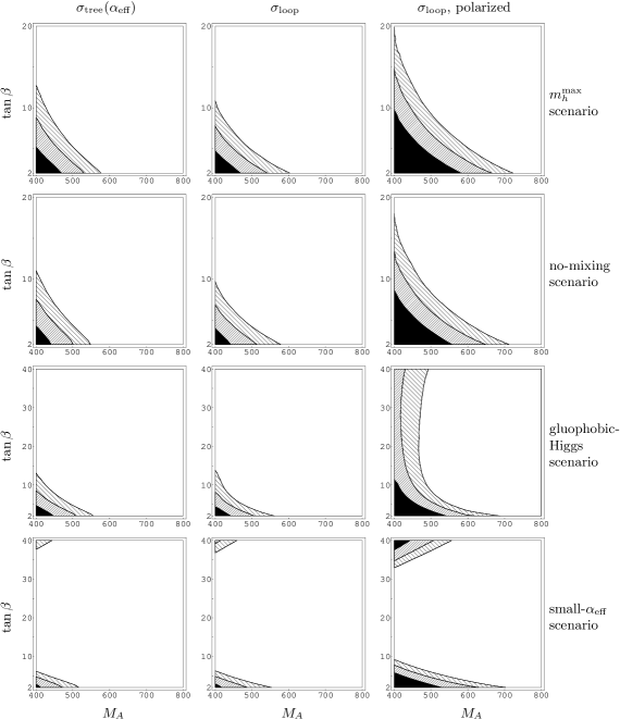
Figure 11: The tree-level cross section for $e^{+}e^{-}\to\bar{\nu}\nu\,H$, $\sigma^{0}_{H}(\alpha_{\rm eff})$, using an $\alpha_{\rm eff}$ approximation (left), and the one-loop cross sections, $\sigma^{1}_{H}$, without (middle), and with beam polarization (right column), are shown in the $M_{A}$–$\tan\beta$ plane for four benchmark scenarios for $\sqrt{s}=1\,\,\mathrm{TeV}$. The different shadings correspond to: white: $\sigma\leq 0.01\mbox{~{}fb}$, light shaded: $0.01\mbox{~{}fb}\leq\sigma\leq 0.02\mbox{~{}fb}$, dark shaded: $0.02\mbox{~{}fb}\leq\sigma\leq 0.05\mbox{~{}fb}$, black: $\sigma\geq 0.05\mbox{~{}fb}$.

In Fig. 11 we first compare the tree-level cross section evaluated in the $\alpha_{\rm eff}$ approximation, $\sigma_{H}^{0}(\alpha_{\rm eff})$ (left column), and the one-loop cross section according to Eq. (34), $\sigma_{H}^{1}$ (middle column), in the four benchmark scenarios. For phenomenological analyses of MSSM Higgs-boson production in this channel the cross section has so far mostly been evaluated using an $\alpha_{\rm eff}$ Born approximation (see also Sect. 4.2).

We concentrate on the case of $\sqrt{s}=1\,\,\mathrm{TeV}$. Since we are interested in $M_{H}\approx M_{A}>\sqrt{s}/2=500\,\,\mathrm{GeV}$, we focus on the region $400\,\,\mathrm{GeV}\leq M_{A}\leq 900\,\,\mathrm{GeV}$, and scan over the whole $\tan\beta$ region. For a LC like TESLA, the anticipated integrated luminosity is of ${\cal O}(2\mbox{ab}^{-1})$. For this luminosity, a production cross section of about $\sigma_{H}=0.01\mbox{~{}fb}$ constitutes a lower limit for the observation of the heavy ${\cal CP}$-even Higgs boson. (For the scenarios discussed below, the dominant decay channel of $H$ is the decay into $t\bar{t}$ or $b\bar{b}$, depending on the value of $\tan\beta$, and also sizable branching ratios into SUSY particles are possible in some regions of parameter space; a more detailed simulation of this process should of course take into account the impact of the decay characteristics on the lower limit of observability, while in this work we use the approximation of a universal limit.) This area is shown in white in Fig. 11. In the four benchmark scenarios shown in Fig. 11, the inclusion of the loop corrections that go beyond the $\alpha_{\rm eff}$ Born approximation turns out to have only a moderate effect on the area in the $M_{A}$–$\tan\beta$ plane in which $H$ production could be observable. While for the $m_{h}^{\rm max}$ and the no-mixing scenario the area is slightly decreased to smaller $\tan\beta$ values and somewhat enlarged to higher $M_{A}$ values, the area is slightly decreased in $\tan\beta$ in the gluophobic-Higgs scenario (and stays approximately the same in $M_{A}$), while the area is slightly enlarged both in $M_{A}$ and $\tan\beta$ in the small-$\alpha_{\rm eff}$ scenario. For the four benchmark scenarios, an observation with $M_{H}>500\,\,\mathrm{GeV}$ is only possible for low $\tan\beta$, $\tan\beta\lesssim 5$, where the LC reach in $M_{H}$ can be extended by up to $100\,\,\mathrm{GeV}$. It should be noted at this point that while the area of observability is modified only slightly in the plots as a consequence of including the loop corrections, the relative changes between the tree-level and the one-loop values of the cross sections can be very large, owing to the suppressed $WWH$ coupling in the tree-level cross section.

The prospects for observing a heavy Higgs boson beyond the kinematical limit of the $HA$ pair production channel become more favorable, however, if polarized beams are used. The cross section becomes enhanced for left-handedly polarized electrons and right-handedly polarized positrons. While a 100% polarization results in a cross section that is enhanced roughly by a factor of 4, more realistic values of 80% polarization for electrons and 60% polarization for positrons [35] would yield roughly an enhancement by a factor of 3. The right column of Fig. 11 shows the four benchmark scenarios with 100% polarization of both beams. The area in the $M_{A}$–$\tan\beta$ plane in which observation of the $H$ boson might become possible is strongly increased in this case. In the $m_{h}^{\rm max}$ and the no-mixing scenario, $H$ observation could be possible for small $\tan\beta$ up to $M_{A}\lesssim 700\,\,\mathrm{GeV}$. In the gluophobic-Higgs and the small-$\alpha_{\rm eff}$ scenario this effect is somewhat smaller. In the latter scenario the discovery of a heavy Higgs boson in the parameter region $M_{A}>500\,\,\mathrm{GeV}$ will become possible also for large $\tan\beta$, $\tan\beta\gtrsim 35$.

While without the inclusion of beam polarization we do not find a significant enhancement of the LC discovery reach as a consequence of the loop corrections in the four benchmark scenarios analyzed in Fig. 11, this behavior changes in other regions of the MSSM parameter space. As a particular example, we investigate the $M_{A}$–$\tan\beta$ plane in the “$\sigma_{H}^{\text{enh}}$” (“enhanced cross section”) scenario, which is defined by

$$M_{\text{SUSY}}=350\,\,\mathrm{GeV},\quad\mu=1000\,\,\mathrm{GeV},$$ (42)

with the other parameters as in the $m_{h}^{\rm max}$ scenario, Eq. (37). The $\sigma_{H}^{\text{enh}}$ scenario is characterized by a relatively small value of $M_{\text{SUSY}}$ and a relatively large value of $\mu$. Large $\tan\beta$ values, $\tan\beta\gtrsim 30$, can result in low and experimentally ruled-out $\tilde{b}$ masses and are therefore omitted.

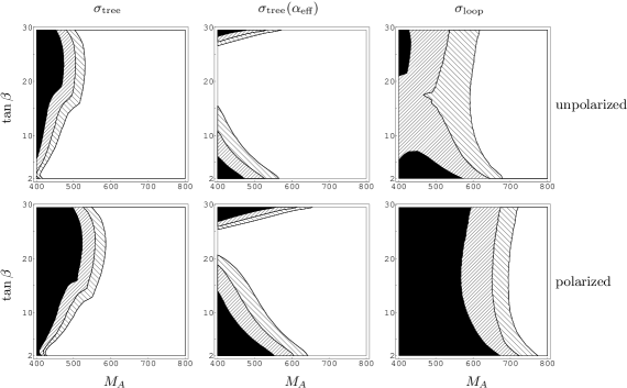
Figure 12: The cross sections for $e^{+}e^{-}\to\bar{\nu}\nu\,H$ are shown in the $M_{A}$–$\tan\beta$ plane for the $\sigma_{H}^{\text{enh}}$ scenario, Eq. (42). The tree-level cross section (left) including the finite wave-function corrections is compared to the $\alpha_{\rm eff}$ approximation (middle) and the one-loop corrected cross section (right column). The upper (lower) row shows the production cross section for unpolarized (100% polarized) electron and positron beams. The color coding is as in Fig. 11.

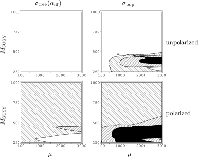
Figure 13: The tree-level cross section for $e^{+}e^{-}\to\bar{\nu}\nu\,H$, $\sigma^{0}_{H}(\alpha_{\rm eff})$, using an $\alpha_{\rm eff}$ approximation (left), and the one-loop cross section, $\sigma^{1}_{H}$ (right column), is shown in the $\mu$–$M_{\text{SUSY}}$ plane for the parameters of Eq. (37) and $M_{A}=600\,\,\mathrm{GeV}$ and $\tan\beta=4$. The upper row shows the unpolarized case, while in the lower row the effects of beam polarization are included. The color coding is as in Fig. 11.

In the upper row of Fig. 12 we compare $\sigma_{H}^{0}$, $\sigma_{H}^{0}(\alpha_{\rm eff})$, and $\sigma_{H}^{1}$ for the parameters of the $\sigma_{H}^{\text{enh}}$ scenario, Eq. (42), in the unpolarized case. The figure shows that both the inclusion of the finite Higgs propagator wave-function corrections as compared to the $\alpha_{\rm eff}$ approximation (left vs. middle column) and of the genuine one-loop corrections (right vs. left column) is very important in this scenario. According to the $\alpha_{\rm eff}$ Born approximation, the parameter area in which observation of $H$ is possible would not be significantly larger than in the benchmark scenarios discussed in Fig. 11. For $M_{A}\gtrsim 500$ GeV, observation of the $H$ boson is only possible for either rather small, $\tan\beta\lesssim 5$, or rather large, $\tan\beta\gtrsim 28$, values of $\tan\beta$. Inclusion of the finite Higgs propagator wave-function corrections, which ensure the correct on-shell properties of the outgoing Higgs boson, changes the situation considerably. While for small and large values of $\tan\beta$ the additional corrections suppress the $e^{+}e^{-}\to\bar{\nu}\nu\,H$ cross section, restricting the $H$ observability to values of $M_{A}$ below 500 GeV, observation of the heavy ${\cal CP}$-even Higgs boson of the MSSM becomes possible for $M_{A}\lesssim 550$ GeV for a significant range of intermediate values of $\tan\beta$. Including also the genuine one-loop corrections (right column) leads to a further drastic enhancement of the parameter space in which the $H$ boson could be observed. The observation of the $H$ boson will be possible in this scenario for all values of $\tan\beta$ if $M_{A}\lesssim 600$ GeV, i.e. the discovery reach of the LC in this case is enhanced by about 100 GeV compared to the $HA$ pair production channel.

The prospects in this scenario for observation of the heavy ${\cal CP}$-even Higgs boson of the MSSM become even more favorable if polarized beams are used. The lower row of Fig. 12 shows the situation with 100% polarization of both beams for the $\sigma_{H}^{\text{enh}}$ scenario, Eq. (42). While in this case the tree-level result (both for the case including the finite wave-function corrections and for the $\alpha_{\rm eff}$ approximation) gives rise to observable rates for $M_{A}\lesssim 600\,\,\mathrm{GeV}$ for a certain range of $\tan\beta$ values only, the further genuine loop corrections enhance the cross section significantly. In this situation the observation of the heavy ${\cal CP}$-even Higgs boson might be possible for values of $M_{A}$ up to about 700–750 GeV for all $\tan\beta$ values, corresponding to an enhancement of the LC reach by more than $200\,\,\mathrm{GeV}$. Cross-section values in excess of $0.05\mbox{~{}fb}$ are obtained in this example for all $\tan\beta$ values for $M_{A}\lesssim 600\,\,\mathrm{GeV}$.

In order to investigate whether this result is a consequence of a very special choice of SUSY parameters or a more general feature, in Fig. 13 we choose the parameters of the $m_{h}^{\rm max}$ scenario for a fixed combination of $M_{A}$ and $\tan\beta$, $M_{A}=600\,\,\mathrm{GeV}$, $\tan\beta=4$, but scan over $\mu$ and $M_{\text{SUSY}}$. The choice $M_{H}\approx M_{A}=600\,\,\mathrm{GeV}$ implies that the $HA$ production channel is clearly beyond the reach of a 1-TeV LC. The upper row of Fig. 13 shows that according to the tree-level cross section (using the $\alpha_{\rm eff}$ approximation) an observable rate for a heavy ${\cal CP}$-even Higgs boson with $M_{A}=600\,\,\mathrm{GeV}$ cannot be found for any of the scanned values of $\mu$ and $M_{\text{SUSY}}$. Inclusion of the further loop corrections changes this situation significantly and gives rise to observable rates in this example for nearly all $M_{\text{SUSY}}\lesssim 500\,\,\mathrm{GeV}$ if $\mu\gtrsim 500\,\,\mathrm{GeV}$. The visible “structure” at $M_{\text{SUSY}}\approx 500\,\,\mathrm{GeV}$ is the result of several competing effects that affect the finite Higgs wave-function corrections.

The same analysis, but with 100% polarization of both beams, is shown in the lower row of Fig. 13. The tree-level $\alpha_{\rm eff}$ approximation results in an observable rate in nearly the whole plane apart from the area with $\mu\gtrsim 1000\,\,\mathrm{GeV}$ and $M_{\text{SUSY}}\lesssim 350\,\,\mathrm{GeV}$. Adding the loop corrections again improves the situation. No unobservable holes remain in the $\mu$–$M_{\text{SUSY}}$ plane, i.e. the heavy ${\cal CP}$-even Higgs boson with $M_{H}\approx 600\,\,\mathrm{GeV}$ should be visible at a 1-TeV LC with (idealized) beam polarization in this scenario. The production cross section is larger than $0.02\mbox{~{}fb}$ for all $\mu$ and $M_{\text{SUSY}}\lesssim 500\,\,\mathrm{GeV}$ and mostly even larger than $0.05\mbox{~{}fb}$ for $\mu\gtrsim 500\,\,\mathrm{GeV}$.

         

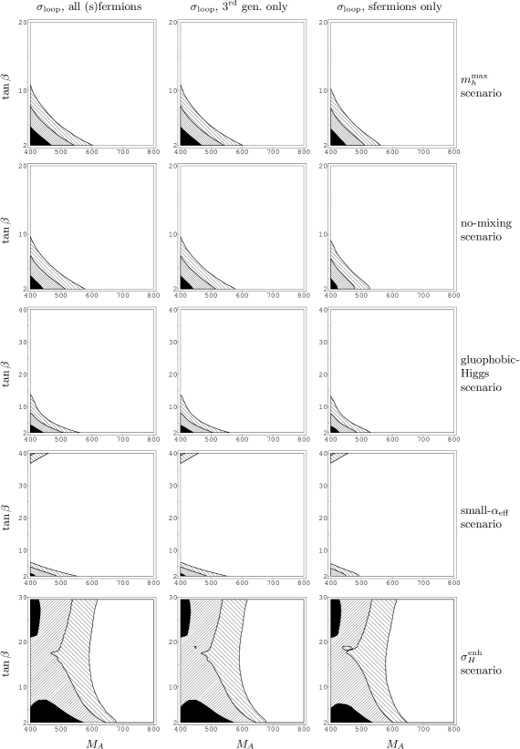
Figure 14: $\sigma_{H}^{1}$ is shown in the $M_{A}$–$\tan\beta$ plane for the four benchmark scenarios defined in Eqs. (37)–(40) and the $\sigma_{H}^{\text{enh}}$ scenario for $\sqrt{s}=1\,\,\mathrm{TeV}$ in the unpolarized case. The one-loop result containing the corrections from all fermion and sfermion loops (left) is compared with the result from only third-generation fermions and sfermions (middle) and the purely sfermionic corrections from all families (right column). The color coding is as in Fig. 11.

In Fig. 14 we compare for all five scenarios analyzed in this paper the results for the cross section when different parts of the generic one-loop corrections are taken into account. In all cases the full result for the Higgs propagator corrections being absorbed in the lowest-order cross section are employed. The left column shows the result containing the corrections from all fermion and sfermion loops, $\sigma_{H}^{1}$, which is repeated from previous plots for comparison purposes. The middle column shows the cross-section prediction based on taking into account only the corrections from the third-generation fermions and sfermions, which have turned out to be the leading corrections for the light Higgs-boson production. The result shown in the right column have been obtained by including only the purely sfermionic contributions from all generations, i.e. the fermion-loop corrections are omitted in this case. As expected from Fig. 11, in the four scenarios defined in Eqs. (37)–(40), where the loop corrections turned out to modify the parameter regions in which $H$ observation becomes possible only slightly, omitting the contributions of the first two generations of fermions and sfermions and of the fermion loops of all three generations does not lead to a qualitative change in the $H$ discovery reach. In the $\sigma_{H}^{\text{enh}}$ scenario, on the other hand, the genuine one-loop corrections had a considerable impact on the area in the $M_{A}$–$\tan\beta$ plane in which $H$ observation is possible, see Fig. 12. The result displayed in the middle column for this scenario shows that the bulk of the corrections comes from the third generation of fermions and sfermions, i.e. omission of the first two generations does not lead to significant effects in the $M_{A}$–$\tan\beta$ plane. The result in the right column for this scenario shows furthermore that the omission of all fermion-loop corrections leads only to very moderate changes of the parameter regions where $H$ observation is possible. As a consequence, the by far dominant corrections in this scenario can be identified as the ones from the sfermions of the third generation. This is contrary to the $h$ production, where we found that the fermionic corrections are mostly larger than the sfermionic ones.

4.4 Comparison with existing results

We have calculated the corrections to the production of both ${\cal CP}$-even Higgs bosons of the MSSM, $h$ and $H$, via the process $e^{+}e^{-}\to\bar{\nu}\nu\,\{h,H\}$. The results for the $h$ production can be compared with the existing result from Ref. [10].

Our calculation differs from the one in Ref. [10] in several respects. Our renormalization differs from the one used in Ref. [10] for the Higgs-boson field-renormalization constants and for $\tan\beta$. Concerning the field-renormalization constants, we incorporate a finite wave-function correction that ensures the correct on-shell properties of the outgoing Higgs boson, while in Ref. [10] the Higgs propagator corrections have been taken into account in an $\alpha_{\rm eff}$ approximation only. Concerning $\tan\beta$, we use the $\overline{\rm{MS}}$ definition that in general leads to a better numerical stability [15, 36]. While in Ref. [10] the contributions from the Higgs-strahlung diagrams have been taken into account in lowest order only, we have incorporated also the loop corrections for this class of diagrams in the same way as for the $WW$-fusion diagrams. Furthermore we have evaluated the corrections from the fermion and sfermion loops of all generations, while in Ref. [10] only the third generation has been taken into account. In Sect. 4.2 it has been shown that relevant corrections can also arise from the first two generations.

We have performed a numerical comparison with the results given in Refs. [10, 37] for the SM and light ${\cal CP}$-even Higgs production in the MSSM, restricting our results to the contributions of the third generation only.

• Our tree-level results show a rather pronounced threshold peak for small values of $\sqrt{s}$, where on-shell production of both the Higgs and the $Z$ boson becomes possible. In this region our results largely differ from those of Ref. [10], while we find very good agreement with the results of Ref. [28]. For large values of $\sqrt{s}$, i.e. far above the threshold, our tree-level results roughly agree with the ones of Ref. [10].

• For the loop corrections in the SM case we find significant deviations with the results of Ref. [10] over the whole parameter space. While the authors of Ref. [10] find large corrections of up to $-15\%$, the corrections in our result for the SM cross section turn out to be moderate and do not exceed $\pm 2\%$ (see Figs. 5–6). The size of the corrections that we find agrees quantitatively with the estimate of the leading term in the heavy-top expansion [38]. As a further cross-check of our results, we compared the SM result at the tree and at the one-loop level (for the third generation only and for all generations) with the one of Ref. [28] and found perfect agreement.

• The same qualitative difference compared to the results of Ref. [10] that we find for the fermion-loop corrections in the SM also occurs for the $h$ production cross section in the MSSM. Again, the fermion-loop corrections in our result turn out to be much smaller than the ones in Ref. [10]. Related to this fact, the relative importance of the corrections from fermion and sfermion loops is different in our result. While in Ref. [10] the relative size of the purely sfermionic corrections does not exceed $+11\%$ of the full correction, we find that the sfermionic corrections can become as large as the purely fermionic ones for large mixing in the scalar top sector.

• In addition to the above-mentioned large deviations, which cannot arise from the use of slightly different renormalization schemes and of different approximations, there are further differences related to the fact that we have implemented the Higgs propagator corrections according to Eqs. (30), (31), while in Ref. [10] an $\alpha_{\rm eff}$ approximation has been used. As shown in Fig. 7, the $\alpha_{\rm eff}$ approximation differs from the full on-shell result by several percent and is therefore not sufficiently accurate in view of the prospective precision reachable at a LC in this channel.

5 Conclusions

We have investigated the production of the ${\cal CP}$-even MSSM Higgs-bosons at a future Linear Collider in the process $e^{+}e^{-}\to\bar{\nu}\nu\,\{h,H\}$. This process is mediated via the $WW$-fusion mechanism, which dominates at higher energies, and via the Higgs-strahlung process, which is important at low energies. We have evaluated all one-loop contributions from fermions and sfermions, and we have furthermore implemented the numerically large process-independent Higgs-boson propagator corrections in such a way that the correct on-shell properties of the outgoing Higgs bosons are ensured.

At a high-energy Linear Collider, the process $e^{+}e^{-}\to\bar{\nu}\nu\,h$ will be the production mode with the highest cross section. For the genuine loop corrections beyond those arising from Higgs propagator contributions, we have found corrections of about 1–5%. These corrections will be relevant in view of the anticipated precision of the cross-section measurement at the LC. The same is true for the deviations between the result containing the full Higgs-boson propagator corrections and the result based on the $\alpha_{\rm eff}$ approximation.

We have also evaluated the correction for the corresponding SM Higgs-production process and found for $M_{H_{\rm SM}}=115\,\,\mathrm{GeV}$ corrections in the range of $+5\%$ for small $\sqrt{s}$, $\sqrt{s}\approx 250\,\,\mathrm{GeV}$, to $-1.2\%$ for large $\sqrt{s}$.

Restricting our result to the contributions from third-generation fermions and sfermions only (and disregarding the correction arising from replacing the $\alpha_{\rm eff}$ approximation by the full Higgs-boson propagator corrections in the MSSM case), we have compared our results for the SM case and for light ${\cal CP}$-even Higgs-boson production in the MSSM with the corresponding results given in Ref. [10]. We find significant deviations both in the overall size of the radiative corrections, which we find to be considerably smaller, and in the relative importance of fermion- and sfermion-loop contributions.

Concerning the production of the heavy ${\cal CP}$-even Higgs boson, we find that in a set of benchmark scenarios proposed for Higgs-boson searches at future colliders, the genuine loop corrections beyond those arising from Higgs propagator contributions only slightly enhance the discovery reach of the Linear Collider. In the case of polarized electron and positron beams, however, the Linear Collider reach can be significantly extended beyond the kinematical limit of the $HA$ pair-production channel. In more favorable regions of the MSSM parameter space, the genuine loop corrections can drastically enlarge the parameter space for which detection of the heavy ${\cal CP}$-even Higgs boson becomes possible. In such a scenario, assuming polarized beams, at $\sqrt{s}=1\,\,\mathrm{TeV}$ the detection of $H$ could be possible up to $M_{H}\approx 750\,\,\mathrm{GeV}$.

Acknowledgements

We thank W. Hollik for helpful discussions. We thank S. Dittmaier, H. Logan, and S. Su for providing us with detailed numbers of their calculations to cross-check our results and for useful discussions. We furthermore thank H. Eberl for helpful communication concerning the comparison of our results. G.W. thanks the Max-Planck Institut für Physik in Munich for the hospitality offered to him during his stay where parts of this work were carried out. This work has been supported by the European Community’s Human Potential Programme under contract HPRN-CT-2000-00149 Physics at Colliders.

References

-
[1]
H.P. Nilles,
Phys. Rep. 110 (1984) 1;
H.E. Haber and G.L. Kane, Phys. Rep. 117, (1985) 75;
R. Barbieri, Riv. Nuovo Cim. 11, (1988) 1. - [2] J. Gunion, H. Haber, G. Kane, and S. Dawson, The Higgs Hunter’s Guide, Addison-Wesley, 1990.
-
[3]
J. Küblbeck, M. Böhm, and A. Denner,
Comput. Phys. Commun. 60 (1990) 165;
T. Hahn, Comput. Phys. Commun. 140 (2001) 418, hep-ph/0012260. - [4] T. Hahn and M. Pérez-Victoria, Comput. Phys. Commun. 118 (1999) 153, hep-ph/9807565.
- [5] M. Carena, S. Heinemeyer, C. Wagner, and G. Weiglein, to appear in Eur. Phys. J. C, hep-ph/0202167.
-
[6]
K. Desch and N. Meyer,
LC-PHSM-2001-025, see
www.desy.de/lcnotes ;
K. Desch, private communication. -
[7]
D. Jones and S. Petcov,
Phys. Lett. B 84 (1979) 440;
R. Cahn and S. Dawson, Phys. Lett. B 136 (1984) 196, [Erratum: ibid. B 138 (1984) 464];
G. Kane, W. Repko, and W. Rolnick, Phys. Lett. B 148 (1984) 367;
R. Cahn, Nucl. Phys. B 255 (1985) 341, [Erratum: ibid. B 262 (1985) 744];
G. Altarelli, B. Mele, and F. Pitolli, Nucl. Phys. B 287 (1987) 205. - [8] W. Kilian, M. Krämer, and P. Zerwas, Phys. Lett. B 373 (1996) 135, hep-ph/9512355.
-
[9]
G. Belanger et al.,
proceedings of the
RADCOR 2002 – Loops and Legs 2002,
Kloster Banz, Germany, Sep. 2002,
hep-ph/0211268;
J. Fujimoto, talk given at the RADCOR 2002 – Loops and Legs 2002;
O. Tarasov, talk given at the RADCOR 2002 – Loops and Legs 2002; see:
www-zeuthen.desy.de/theory/radcor02/Hagedorn/list_of_transparencies.html. - [10] H. Eberl, W. Majerotto, and V. Spanos, Phys. Lett. B 538 (2002) 353, hep-ph/0204280; hep-ph/0210038.
- [11] A. Arhrib, hep-ph/0207330.
-
[12]
S. Heinemeyer, W. Hollik, J. Rosiek, and G. Weiglein,
Eur. Phys. J. C 19 (2001) 535,
hep-ph/0102081;
S. Heinemeyer and G. Weiglein, Nucl. Phys. Proc. Suppl. 89 (2000) 210; hep-ph/0102177. -
[13]
H. Logan and S. Su,
Phys. Rev. D 66 (2002) 035001,
hep-ph/0203270;
hep-ph/0206135.
S. Su, hep-ph/0210448. -
[14]
A. Arhrib, M. Capdequi Peyranere, W. Hollik, and
G. Moultaka,
Nucl. Phys. B 581 (2000) 34,
hep-ph/9912527.
O. Brein, hep-ph/0209124. - [15] M. Frank, S. Heinemeyer, W. Hollik, and G. Weiglein, hep-ph/0202166; in preparation.
-
[16]
W. Siegel,
Phys. Lett. B 84 (1979) 193;
D. Capper, D. Jones, and P. van Nieuwenhuizen, Nucl. Phys. B 167 (1980) 479. - [17] A. Djouadi, D. Haidt, B. Kniehl, B. Mele, and P. Zerwas, in the Proceedings of the Workshop Collisions at 500 GeV: The Physics Potential, Munich–Annecy–Hamburg, ed. P. Zerwas, DESY 92-123A,B; 93-123C.
- [18] A. Denner, Fortsch. Phys. 41 (1993) 307.
-
[19]
P. Chankowski, S. Pokorski, and J. Rosiek,
Phys. Lett. B 286 (1992) 307;
Nucl. Phys. B 423 (1994) 423,
hep-ph/9303309;
A. Dabelstein, Z. Phys. C 67 (1995) 495, hep-ph/9409375. - [20] S. Heinemeyer, W. Hollik, and G. Weiglein, Phys. Rev. D 58 (1998) 091701, hep-ph/9803277; Phys. Lett. B 440 (1998) 296, hep-ph/9807423.
- [21] S. Heinemeyer, W. Hollik, and G. Weiglein, Eur. Phys. J. C 9 (1999) 343, hep-ph/9812472.
-
[22]
G. Degrassi, P. Slavich, and F. Zwirner,
Nucl. Phys. B 611 (2001) 403,
hep-ph/0105096;
A. Brignole, G. Degrassi, P. Slavich, and F. Zwirner, Nucl. Phys. B 631 (2002) 195, hep-ph/0112177. -
[23]
S. Heinemeyer, W. Hollik, and G. Weiglein,
Comput. Phys. Comm. 124 (2000) 76,
hep-ph/9812320;
hep-ph/0002213;
M. Frank, S. Heinemeyer, W. Hollik, and G. Weiglein, hep-ph/0202166;
see www.feynhiggs.de. - [24] S. Heinemeyer, W. Hollik, and G. Weiglein, Eur. Phys. J. C 16 (2000) 139, hep-ph/0003022.
- [25] T. Hahn, Nucl. Phys. Proc. Suppl. 89 (2000) 231, hep-ph/0005029.
- [26] T. Hahn and C. Schappacher, Comput. Phys. Commun. 143 (2002) 54, hep-ph/0105349.
-
[27]
G. van Oldenborgh and J. Vermaseren,
Z. Phys. C 46 (1990) 425;
G. van Oldenborgh, Comput. Phys. Commun. 66 (1991) 1. - [28] S. Dittmaier, private communication.
- [29] G.P. Lepage, J. Comput. Phys. 27 (1978) 192.
- [30] J. Berntsen, T. Espelid, and A. Genz, ACM Trans. Math. Software 17 (1991) 452, see also doi.acm.org/10.1145/210232.210234 .
- [31] G. Degrassi, S. Heinemeyer, W. Hollik, P. Slavich, and G. Weiglein, in preparation.
-
[32]
J. Aguilar-Saavedra et al.,
TESLA TDR Part 3:
“Physics at an Linear Collider,”
hep-ph/0106315,
see: tesla.desy.de/tdr ;
T. Abe et al. [American Linear Collider Working Group Collaboration], “Linear collider physics resource book for Snowmass 2001,” hep-ex/0106056;
K. Abe et al. [ACFA LC Working Group Collaboration], hep-ph/0109166. -
[33]
T. Appelquist and J. Carazzone,
Phys. Rev. D 11 (1975) 2856;
A. Dobado, M. Herrero, and S. Peñaranda, Eur. Phys. Jour. C 7 (1999) 313, hep-ph/9710313, Eur. Phys. Jour. C 12 (2000) 673, hep-ph/9903211; Eur. Phys. Jour. C 17 (2000) 487, hep-ph/0002134. -
[34]
A. Djouadi, P. Gambino, S. Heinemeyer, W. Hollik,
C. Jünger, and G. Weiglein,
Phys. Rev. Lett. 78 (1997) 3626,
hep-ph/9612363;
Phys. Rev. D 57 (1998) 4179,
hep-ph/9710438;
S. Heinemeyer and G. Weiglein, JHEP 0210 (2002) 072, hep-ph/0209305; proceedings of the RADCOR2000, Carmel, Sep. 2000, hep-ph/0102317. -
[35]
TESLA TDR Part 2: “The Accelerator,”
see tesla.desy.de/tdr ;
G. Moortgat-Pick and H. Steiner, Eur. Phys. J. direct C 6 (2001) 1, hep-ph/0106155. - [36] A. Freitas and D. Stöckinger, hep-ph/0205281.
- [37] H. Eberl, private communication.
- [38] B. Kniehl and M. Spira, Z. Phys. C 69 (1995) 77, hep-ph/9505225.