Rare $B_{s}\rightarrow\gamma\,\nu\bar{\nu}$ decay with polarized photon and new physics effects

Abstract

Using the most general, model independent effective Hamiltonian, the rare $B_{s}\rightarrow\gamma\,\nu\bar{\nu}$ decay with polarized photon is studied. The sensitivity of the branching ratio and photon polarization to the new Wilson coefficients are investigated. It is shown that these physical observables are sensitive to the vector and tensor type interactions, which would be useful in search of new physics.

PACS number(s): 12.60.–i, 13.20.–v, 13.20.He

1 Introduction

Since the first observation of the flavor–changing neutral current induced decays $B\rightarrow X_{s}\gamma$ and $B\rightarrow K^{*}\gamma$ by CLEO [1], the rare B-meson decays have begun to play a more important role in the particle physics phenomenology. This can be attributed to the fact that as these processes only occur at loop level in the weak interaction, they provide fertile testing ground for the gauge sector of the SM. In addition, these decays can also serve as a good probe for establishing new physics beyond the SM.

From experimental point of view, studying rare $B$ meson decays can provide essential information about the poorly known parameters of the SM, such as the elements of the Cabibbo–Kobayashi–Maskawa (CKM) matrix, the leptonic decay constants etc. In this connection, the pure leptonic B decays $B\rightarrow\ell^{+}\ell^{-}$ could be used to get such information. However, these decays are proportional to the lepton mass, so that they are helicity suppressed with the factor of $m^{2}_{\ell}/m^{2}_{B}$, having the branching ratios of $BR(B_{s}\rightarrow e^{+}e^{-},\mu^{+}\mu^{-})\simeq 10^{-14},10^{-9}$ [2]. For $\tau$ channel, there is no such suppression and $BR(B_{s}\rightarrow\tau^{+}\tau^{-})\simeq 10^{-7}$ [3], but this time the difficulty arises from their experimental observation due to the low efficiency. As for the $B\rightarrow\nu\bar{\nu}$ decay, it is obviously forbidden in the SM due to the helicity conservation if neutrino is massless. Alternatively, the $B\rightarrow\gamma\,\nu\bar{\nu}$ decays can be considered as potential processes to determine the above-mentioned constants, especially the leptonic decay constant $f_{B}$, since its branching ratio (BR) quadratically depends on this constant. Due to the additional the photon emission in $B\rightarrow\gamma\,\nu\bar{\nu}$, the helicity suppression is removed, as in $B\rightarrow\gamma\,\ell^{+}\ell^{-}$ decay, so that larger BR is expected. The SM prediction for $BR(B_{s}\rightarrow\gamma\,\nu\bar{\nu})$ is of the order of $\sim 10^{-8}$ and it has very clear experimental signature, i.e., the ”missing mass” and isolated photon so that they are among the potentially measurable decays in the near future.

In this paper, we will use the light cone QCD sum rules method to evaluate the hadronic matrix elements and study the rare $B_{s}\rightarrow\gamma\,\nu\bar{\nu}$ decay in a general model independent way by taking into account the polarization effects of the photon. $B\rightarrow\gamma\,\nu\bar{\nu}$ decay has been investigated in the SM, using the constituent quark model and pole models [4] for the determination of the leptonic decay constants $f_{B}$. In [5], this process was studied also within the framework of the light cone QCD sum rules method, but there neutrino was assumed to be massless and the Hamiltonian consisted of a single term representing the four vector interactions of the left handed neutrinos only. However, the Super Kamiokande [6] results indicated that neutrino had mass so that it could have right components. Therefore, in our work, we use a most general model independent effective Hamiltonian, which contains the scalar and tensor type interactions as well as the vector types (See Eq.(2) below). We note that this mode has been studied in a recent work [7] in a similar way to our analysis and shown that the spectrum is sensitive to the types of the interactions so that it is useful to discriminate the various new physics effects.

In a radiative decay mode like ours, the final state photon can emerge with a definite polarization and studying the effects of polarized photon may provide another kinematical variable, in addition to the differential and total branching ratios for radiative decays [8]. Although experimental measurement of this variable would be much more difficult than that of e.g., polarization of the final leptons in $B\rightarrow\gamma\,\ell^{+}\ell^{-}$ decay, this is still another kinematical variable for studying radiative decays. In this work we will investigate sensitivity of such ”photon polarization asymmetry” in $B_{s}\rightarrow\gamma\,\nu\bar{\nu}$ decay to the new Wilson coefficients.

The paper is organized as follows: In section 2, we present the most general, model independent form of the effective Hamiltonian and the parametrization of the hadronic matrix elements in terms of appropriate form factors. We then calculate the differential decay width and the photon polarization asymmetry for the $B_{s}\rightarrow\gamma\,\nu\bar{\nu}$ decay when the photon is in positive and negative helicity states . Section 3 is devoted to the numerical analysis and discussion of our results.

2 Matrix element for the $B_{s}\rightarrow\gamma\,\nu\bar{\nu}$ decay

For the semileptonic $B_{s}\rightarrow\gamma\,\nu\bar{\nu}$ decay, the basic quark level process is $b\rightarrow s\nu\bar{\nu}$, which can be written in terms of 10 model independent four–Fermi interactions in the following form [9]-[11]:

$${\cal H}_{eff} = \frac{\alpha\,G_{F}}{4\sqrt{2}\pi}\frac{V_{tb}V_{ts}^{\ast}}{\sin^{2}\theta_{W}}\Bigg{\{}C_{LL}^{tot}\,\bar{s}\gamma_{\mu}(1-\gamma_{5})b\,\bar{\nu}\gamma^{\mu}(1-\gamma_{5})\nu+C_{LR}^{tot}\,\bar{s}\gamma_{\mu}(1-\gamma_{5})b\,\bar{\nu}\gamma^{\mu}(1+\gamma_{5})\nu$$

$$+C_{RL}\,\bar{s}\gamma_{\mu}(1+\gamma_{5})b\,\bar{\nu}\gamma^{\mu}(1-\gamma_{5})\nu+C_{RR}\,\bar{s}\gamma_{\mu}(1+\gamma_{5})b\,\bar{\nu}\gamma^{\mu}(1+\gamma_{5})\nu$$

$$+C_{LRLR}\,\bar{s}(1+\gamma_{5})b\,\bar{\nu}(1+\gamma_{5})\nu+C_{RLLR}\,\bar{s}(1-\gamma_{5})b\,\bar{\nu}(1+\gamma_{5})\nu$$

$$+C_{LRRL}\,\bar{s}(1+\gamma_{5})b\,\bar{\nu}(1-\gamma_{5})\nu+C_{RLRL}\,\bar{s}(1-\gamma_{5})b\,\bar{\nu}(1-\gamma_{5})\nu$$

$$+C_{T}\,\bar{s}\sigma_{\mu\nu}b\,\bar{\nu}\sigma^{\mu\nu}\nu+iC_{TE}\,\epsilon^{\mu\nu\alpha\beta}\bar{s}\sigma_{\mu\nu}b\,\bar{\nu}\sigma_{\alpha\beta}\nu\Bigg{\}}~{},$$

where $C_{X}$ are the coefficients of the four–Fermi interactions with $X=LL,LR,RL,RR$ describing vector, $X=LRLR,RLLR,LRRL,RLRL$ scalar and $X=T,TE$ tensor type interactions. The Wilson coefficients $C_{LL}$ and $C_{LR}$ already exist in the SM in the form $C_{9}^{eff}-C_{10}$ and $C_{9}^{eff}+C_{10}$ for the $b\rightarrow s\ell^{+}\ell^{-}$ decay, while for $b\rightarrow s\nu\bar{\nu}$ transition, we have $C_{9}=-C_{10}=X(x_{t})$ [12] with

$$X(x_{t}) = \frac{x_{t}}{8}\Bigg{[}\frac{x_{t}+2}{x_{t}-1}+\frac{3(x_{t}-2)}{(x_{t}-1)^{2}}\ln(x_{t})\Bigg{]}+\frac{\alpha_{s}}{4\pi}\,X_{1}(x_{t})\,.$$ (1)

Here, $x_{t}=m^{2}_{t}/m^{2}_{W}$ and $X_{1}(x_{t})$, which gives about $3\%$ contribution to $C_{9}$, can be found in [3]. Now, writing

$$C_{LL}^{tot} = 2X(x_{t})+C_{LL}~{},$$

$$C_{LR}^{tot} = C_{LR}~{},$$

we see that $C_{LL}^{tot}$ contains the contributions from the SM and also from the new physics. We note that the Wilson coefficients $C_{LRLR}$, $C_{RLLR}$, $C_{LRRL}$ and $C_{RLRL}$ in Eq.(2) describe the scalar type interactions, which do not contribute for the $B_{s}\rightarrow\gamma\,\nu\bar{\nu}$ processes.

The next step is, starting with the Hamiltonian in Eq.(2), to calculate the $B_{s}\rightarrow\gamma\,\nu\bar{\nu}$ decay at hadronic level. We already note that the pure leptonic decay $B_{s}\rightarrow\nu\bar{\nu}$ is forbidden due to helicity conservation. However, when a photon is emitted from initial b or s-quark lines, this pure leptonic process change into the corresponding radiative one and no helicity suppression exists anymore. The contributions coming from the release of a free photon from any internal charged line will be suppressed by a factor of $m^{2}_{b}/m^{2}_{W}$, therefore they can be neglected. Thus, the matrix elements necessary to calculate $B_{s}\rightarrow\gamma\,\nu\bar{\nu}$ decay are as follows [13]-[15]:

$$\langle\gamma(k)\left|\bar{s}\gamma_{\mu}(1\mp\gamma_{5})b\right|B(p_{B})\rangle = \frac{e}{m_{B}^{2}}\Big{\{}\epsilon_{\mu\nu\lambda\sigma}\varepsilon^{\ast\nu}q^{\lambda}k^{\sigma}g(q^{2})$$ (2)

$$\pm i\,\Big{[}\varepsilon^{\ast}_{\mu}(kq)-(\varepsilon^{\ast}q)k_{\mu}\Big{]}f(q^{2})\Big{\}}~{},$$

$$\langle\gamma(k)\left|\bar{s}\sigma_{\mu\nu}b\right|B(p_{B})\rangle = \frac{e}{m_{B}^{2}}\epsilon_{\mu\nu\lambda\sigma}\Big{[}G\varepsilon^{\ast\lambda}k^{\sigma}+H\varepsilon^{\ast\lambda}q^{\sigma}+N(\varepsilon^{\ast}q)q^{\lambda}k^{\sigma}\Big{]}~{},$$ (3)

$$\langle\gamma(k)\left|\bar{q}(1\mp\gamma_{5})b\right|B(p_{B})\rangle = 0~{},$$ (4)

where $\varepsilon_{\mu}^{\ast}$ and $k_{\mu}$ are the four vector polarization and four momentum of the photon, respectively, $q$ is the momentum transfer and $p_{B}$ is the momentum of the $B$ meson. Due to Eq.(4), the scalar type interactions do not contribute to the $B_{s}\rightarrow\gamma\,\nu\bar{\nu}$ decay, as we have noted before. Using eqs.(2-4), the matrix element for $B_{s}\rightarrow\gamma\,\nu\bar{\nu}$ decay can be calculated as follows:

$${\cal M} = \frac{\alpha G_{F}}{4\sqrt{2}\,\pi}\frac{V_{tb}V_{ts}^{*}}{\sin^{2}\theta_{W}}\frac{e}{m_{B}^{2}}\,\Bigg{\{}\bar{\nu}\gamma^{\mu}(1-\gamma_{5})\nu\,\Big{[}A_{1}\epsilon_{\mu\nu\alpha\beta}\varepsilon^{\ast\nu}q^{\alpha}k^{\beta}+i\,A_{2}\Big{(}\varepsilon_{\mu}^{\ast}(kq)-(\varepsilon^{\ast}q)k_{\mu}\Big{)}\Big{]}$$

$$+ \bar{\nu}\gamma^{\mu}(1+\gamma_{5})\nu\,\Big{[}B_{1}\epsilon_{\mu\nu\alpha\beta}\varepsilon^{\ast\nu}q^{\alpha}k^{\beta}+i\,B_{2}\Big{(}\varepsilon_{\mu}^{\ast}(kq)-(\varepsilon^{\ast}q)k_{\mu}\Big{)}\Big{]}$$

$$+ i\,\epsilon_{\mu\nu\alpha\beta}\bar{\nu}\sigma^{\mu\nu}\nu\,\Big{[}G\varepsilon^{\ast\alpha}k^{\beta}+H\varepsilon^{\ast\alpha}q^{\beta}+N(\varepsilon^{\ast}q)q^{\alpha}k^{\beta}\Big{]}$$

$$+ i\,\bar{\nu}\sigma_{\mu\nu}\nu\,\Big{[}G_{1}(\varepsilon^{\ast\mu}k^{\nu}-\varepsilon^{\ast\nu}k^{\mu})+H_{1}(\varepsilon^{\ast\mu}q^{\nu}-\varepsilon^{\ast\nu}q^{\mu})+N_{1}(\varepsilon^{\ast}q)(q^{\mu}k^{\nu}-q^{\nu}k^{\mu})\Big{]}\Bigg{\}}~{},$$

where

$$A_{1} = (C_{LL}^{tot}+C_{RL})g~{}~{}~{},~{}~{}~{}$$

$$A_{2} = (C_{LL}^{tot}-C_{RL})f~{},$$

$$B_{1} = (C_{LR}^{tot}+C_{RR})g~{},$$

$$B_{2} = (C_{LR}^{tot}-C_{RR})f~{},$$

$$G = 4C_{T}g_{1}~{},$$

$$N = -4C_{T}\frac{1}{q^{2}}(f_{1}+g_{1})~{},$$ (6)

$$H = N(qk)~{},$$

$$G_{1} = -8C_{TE}g_{1}~{},$$

$$N_{1} = 8C_{TE}\frac{1}{q^{2}}(f_{1}+g_{1})~{},$$

$$H_{1} = N_{1}(qk)$$

The next task is the calculation of the differential decay rate of $B_{s}\rightarrow\gamma\,\nu\bar{\nu}$ decay as a function of dimensionless parameter $x=2E_{\gamma}/m_{B}$, where $E_{\gamma}$ is the photon energy. In such a radiative decay, the final state photon can emerge with a definite polarization and there follows the question of how sensitive the branching ratio is to the new Wilson coefficients when the photon is in the positive or negative helicity states. To find an answer to this question, we evaluate $\frac{d\Gamma(\varepsilon^{\ast}=\varepsilon_{1})}{dx}$ and $\frac{d\Gamma(\varepsilon^{\ast}=\varepsilon_{2})}{dx}$ for $B_{s}\rightarrow\gamma\,\nu\bar{\nu}$ decay, in the c.m. frame of $\nu\bar{\nu}$, in which four-momenta and polarization vectors ,$\varepsilon_{1}$ and $\varepsilon_{2}$, are as follows:

$$P_{B} = (E_{B},0,0,E_{k})\,\,\,,\,\,\,k=(E_{k},0,0,E_{k})\,\,\,,\,\,\,p_{1}=(p,0,p\sqrt{1-z^{2}},-pz)$$

$$p_{2} = (p,0,-p\sqrt{1-z^{2}},pz)\,\,\,,\,\,\,\varepsilon_{1}=(0,1,i,0)/\sqrt{2}\,\,\,,\,\,\,\varepsilon_{2}=(0,1,-i,0)/\sqrt{2}$$ (7)

where $E_{B}=m_{B}(2-x)/2\sqrt{1-x}$, $E_{k}=m_{B}x/2\sqrt{1-x}$, and $p=m_{B}\sqrt{1-x}/2$. In Eq.(7) $z=\cos\theta$, where $\theta$ is the angle between the momentum of the B-meson and that of $\nu$ in the c.m. frame of $\nu\bar{\nu}$. Using the above forms, obtain

$$\frac{d\Gamma(\varepsilon^{\ast}=\varepsilon_{i})}{dx} = \,\left|\frac{\alpha G_{F}}{4\sqrt{2}\,\pi}\frac{V_{tb}V_{ts}^{*}}{\sin^{2}\theta_{W}}\right|^{2}\,\frac{\alpha}{\left(2\,\pi\right)^{3}}\,\frac{\pi}{4}\,m_{B}\,\Delta(\varepsilon_{i})$$ (8)

where

$$\Delta(\varepsilon_{i}) = \frac{1}{3}x\,\Bigg{\{}(1-x)\Bigg{[}x^{2}\,m_{B}^{2}\Big{(}\left|A_{1}\right|^{2}+\left|A_{2}\right|^{2}+\left|B_{1}\right|^{2}+\left|B_{2}\right|^{2}\pm 2\,\mbox{\rm Re}[A_{1}A_{2}^{\ast}+B_{1}B_{2}^{\ast}]\Big{)}$$ (9)

$$- 4\Big{(}(-1+x)(\left|H_{1}\right|^{2}+\left|H\right|^{2})+x(\pm\mbox{\rm Im}[G_{1}H^{\ast}-GH_{1}^{\ast}]-\mbox{\rm Re}[G_{1}H_{1}^{\ast}+GH^{\ast}])\Big{)}\Bigg{]}$$

$$+ 2x^{2}\Big{(}\left|G_{1}\right|^{2}+\left|G\right|^{2}\pm 2\,\mbox{\rm Im}[-G_{1}G^{\ast}]\Big{)}\Bigg{\}}$$

with $+(-)$ is for $i=1(2)$.

The effects of polarized photon can be also studied through a variable ”photon polarization asymmetry”, [8]:

$$H(x)=\frac{\frac{d\Gamma(\varepsilon^{\ast}=\varepsilon_{1})}{dx}-\frac{d\Gamma(\varepsilon^{\ast}=\varepsilon_{2})}{dx}}{\frac{d\Gamma(\varepsilon^{\ast}=\varepsilon_{1})}{dx}+\frac{d\Gamma(\varepsilon^{\ast}=\varepsilon_{2})}{dx}} = \frac{\Delta(\varepsilon_{1})-\Delta(\varepsilon_{2})}{\Delta_{0}}\,,$$ (10)

where

$$\Delta(\varepsilon_{1})-\Delta(\varepsilon_{2})=\frac{4}{3}x^{2}\Bigg{\{}(1-x)\Big{(}m^{2}_{B}x\mbox{\rm Re}[A_{1}A_{2}^{\ast}+B_{1}B_{2}^{\ast}]+2\mbox{\rm Im}[GH_{1}^{\ast}-G_{1}H^{\ast}]\Big{)}-2x\mbox{\rm Im}[G_{1}G^{\ast}]\Bigg{\}}$$ (11)

and

$$\Delta_{0} = x^{3}\,\Bigg{\{}\frac{2}{3}m_{B}^{2}(1-x)\,\Big{(}\left|A_{1}\right|^{2}+\left|A_{2}\right|^{2}+\left|B_{1}\right|^{2}+\left|B_{2}\right|^{2}\Big{)}+\frac{4}{3}\,\Big{(}\left|G_{1}\right|^{2}+\left|G\right|^{2}\Big{)}$$ (12)

$$+ 4\frac{(1-x)}{x^{2}}\Big{(}(1-x)(\left|H_{1}\right|^{2}+\left|H\right|^{2})+x\mbox{\rm Re}[G_{1}H_{1}^{\ast}+GH^{\ast}]\Big{)}$$

$$- \frac{1}{3}m_{B}^{2}(1-x)\Big{(}2\mbox{\rm Re}[GN^{\ast}+G_{1}N_{1}^{\ast}]+m^{2}_{B}(1-x)\Big{(}\left|N_{1}\right|^{2}+\left|N\right|^{2}\Big{)}\Big{)}\Bigg{\}}$$

3 Numerical analysis and discussion

In this section we will present our numerical analysis about the branching ratio (BR) and the photon polarization asymmetry $H$ for $B_{s}\rightarrow\gamma\,\nu\bar{\nu}$ decay. It follows from Eqs. (8) and (11) that in order to make such numerical predictions, we first of all need the explicit forms of the form factors $g,~{}f,~{}g_{1}$ and $f_{1}$. They are calculated in framework of light–cone $QCD$ sum rules in [13, 14], in terms of two parameters $F(0)$ and $m_{F}$ as

$$F(q^{2}) = \frac{F(0)}{\left(1-\frac{(1-x)m^{2}_{B}}{m^{2}_{F}}\right)^{2}}$$ (13)

where the values $F(0)$ and $m_{F}$ for the $B_{s}\rightarrow\gamma$ transition are listed in Table 1.

$$\begin{array}[]{|l|cc|}\hline\cr&F(0)&m_{F}\\ \hline\cr g&\phantom{-}1\,GeV&5.6\,GeV\\ f&\phantom{-}0.8\,GeV&6.5\,GeV\\ g_{1}&\phantom{-}3.74\,GeV^{2}&6.4\,GeV\\ f_{1}&\phantom{-}0.68\,GeV^{2}&5.5\,GeV\\ \hline\cr\end{array}$$

Table 1: $B$ meson decay form factors in the light-cone QCD sum rule.

The values of the other input parameters which have been used in the present work are: $m_{B_{s}}=5.28~{}GeV$, $\tau(B_{s})=1.61\times 10^{-12}~{}s$, $\left|V_{tb}V_{ts}^{\ast}\right|=0.045$, $\alpha^{-1}=137$, $G_{F}=1.17\times 10^{-5}~{}GeV^{-2}$, $C_{9}=1.618$. Furthermore we assume in this work that all new Wilson coefficients are real and vary in the region $-4\leq C_{X}\leq 4$. We note that such a choice for the range of the new Wilson coefficients follows from the experimental bounds on the branching ratios of the $B_{s}\rightarrow K^{\ast}\mu^{+}\mu^{-}$ and $B_{s}\rightarrow\mu^{+}\mu^{-}$ decays [16].

For reference, we first present our SM prediction, $BR(B_{s}\rightarrow\gamma\nu\bar{\nu})=9.54\times 10^{-8}$, which is in a good agreement with the result of ref. [5].

In Figs. (1) and (2), we present the dependence of the $BR^{(1)}$ and $BR^{(2)}$ for $B_{s}\rightarrow\gamma\nu\bar{\nu}$ decay on the new Wilson coefficients, $C_{LL}$,$C_{RR}$,$C_{LR}$,$C_{RL}$,$C_{T}$ and $C_{TE}$, where the superscripts $(1)$ and $(2)$ correspond to the positive and negative helicity states of photon, respectively. We observe from these figures that among the new interactions considered in the effective Hamiltonian the branching ratio in both cases is most sensitive to the tensor type of interactions. Indeed, e.g., for $C_{T}(C_{TE})=\pm 2$, $BR^{(1)}$ is larger about $3(8)$ times compared to that of the SM prediction. For $BR^{(2)}$, we get even larger enhancement, which is about $12(45)$ times compared to the SM. In addition, the dependence of the branching ratio in both cases on $C_{T}$ and $C_{TE}$ is symmetrical with respect to the zero point. From Figs.(1) and (2), we also see that branching ratio $BR^{(1)}$ is sensitive to the vector interactions with coefficients $C_{LL}$ and $C_{LR}$, while $BR^{(2)}$ is more sensitive to the coefficients $C_{RR}$ and $C_{RL}$.

In Fig.(3), we present the dependence of the integrated photon polarization asymmetry $H$ for $B_{s}\rightarrow\gamma\nu\bar{\nu}$ decay on the new Wilson coefficients, $C_{LL}$,$C_{RR}$,$C_{LR}$,$C_{RL}$,$C_{T}$ and $C_{TE}$. We see that spectrum of $H$ is perfectly symmetrical with respect to the zero point for all the new Wilson coefficients, except the $C_{RL}$. The coefficient $C_{RL}$, when it is between $-2$ and $0$, is also the only one which gives the constructive contribution to the SM prediction of $H$, which we find $H(B_{s}\rightarrow\gamma\nu\bar{\nu})=0.73$. This behavior is clear also from Fig.(4), in which we plot the differential photon polarization asymmetry $H(x)$ for the same decay as a function of dimensionless variable $x=2E_{\gamma}/m_{B}$ for the different values of the vector interaction with coefficients $C_{RL}$. Finally, we give in Fig.(5), $H(x)$ as a function of $x$ for the different values of the tensor interaction with coefficients $C_{TE}$. From these two last figures, we can conclude that performing measurement of $H$ at different photon energies can give information about the signs of the new Wilson coefficients, as well as their magnitudes.

In conclusion, we have studied the branching ratio of the $B_{s}\rightarrow\gamma\nu\bar{\nu}$ decay when photon has positive and negative helicities, also another physically measurable quantity, namely the photon polarization asymetry of the same decay, using a general, model independent effective Hamiltonian. It follows that these physical observables are very sensitive to the existence of new Wilson coefficients so that their experimental measurements can give valuable information about new physics.

We would like to thank T. M. Aliev and M. Savcı for useful discussions.

Figure 1: The dependence of the integrated branching ratio $BR^{(1)}$ on the new Wilson coefficients for the $B_{s}\rightarrow\gamma\nu\bar{\nu}$ decay. The superscript $(1)$ corresponds to the photon in positive helicity state.

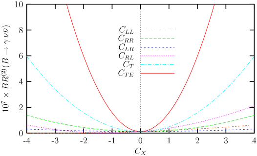
Figure 2: The same as Fig.(1), but for the photon in negative helicity state.

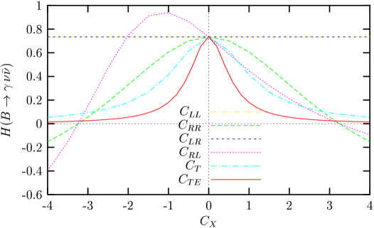
Figure 3: The dependence of the integrated photon polarization asymmety of the $B_{s}\rightarrow\gamma\nu\bar{\nu}$ decay on the new Wilson coefficients.

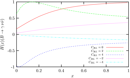
Figure 4: The dependence of the differential photon polarization asymmety of the $B_{s}\rightarrow\gamma\nu\bar{\nu}$ decay on $x$ for different values of $C_{RL}$.

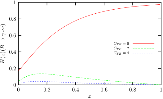
Figure 5: The dependence of the differential photon polarization asymmety of the $B_{s}\rightarrow\gamma\nu\bar{\nu}$ decay on $x$ for different values of $C_{TE}$.

References

• [1] CLEO Collaboration, R. Ammar et al., Phys. Rev. Lett. 71 (1993) 674; CLEO Collaboration, M. S. Alam et al., Phys. Rev. Lett. 74 (1995) 2885.
• [2] G. Eilam, Cai-Dian LΓΌ, and Da-Xin Zang, Phys. Lett. B 391 (1997) 461.
• [3] G. Buchalla, and A. J. Buras , Nucl. Phys. B 400 (1993) 225.
• [4] C. D. LΓΌ, D. X. Zhang, Phys. Lett. B381 (1996) 348.
• [5] T. M. Aliev, A. Γ–zpineci and M. SavcΔ±, Phys. Lett. B393 (1997) 143.
• [6] Super-Kamiokande Collaboration, Y. Fukuda at al., Phys. Rev. Lett. 81 (1998) 1562; CLEO Collaboration, M. S. Alam at al., Phys. Rev. Lett. 74 (1995) 2885.
• [7] O. Cakir and B. SirvanlΔ±, hep-ph/0210019 .
• [8] S. Rai Choudhury and N. Gaur, hep-ph/0205076.
• [9] T. M. Aliev, C. S. Kim, Y. G. Kim, Phys. Rev. D62 (2000) 014026.
• [10] T. M. Aliev, D. A. Demir, M. SavcΔ±, Phys. Rev. D62 (2000) 074016.
• [11] S. Fukae, C. S. Kim, T. Morozumi, T. Yoshikawa, Phys. Rev. D59 (1999) 074013.
• [12] T. Inami and C. S. Lim, Prog. Theor. Phys. 65 (1981) 287.
• [13] G. Eilam, I. Halperin and R. R. Mendel Phys. Lett. B361 (1995) 137.
• [14] T. M. Aliev, A. Γ–zpineci and M. SavcΔ±, Phys. Rev. D55 (1997) 7059.
• [15] T. M. Aliev, A. Γ–zpineci and M. SavcΔ±, Phys. Lett. B520 (2001) 69.
• [16] T. Affolder, et al., CDF Collaboration, Phys. Rev. Lett. 83 (1999) 3278; Yongsheng Gao, CLEO Collaboration, hep-ex/0108005.
Refer to caption