Numerical evaluation of master integrals from differential equations

Abstract

The 4-th order Runge-Kutta method in the complex plane is proposed for numerically advancing the solutions of a system of first order differential equations in one external invariant satisfied by the master integrals related to a Feynman graph. The particular case of the general massive 2-loop sunrise self-mass diagram is analyzed. The method offers a reliable and robust approach to the direct and precise numerical evaluation of master integrals.

1 Introduction

The very high precision of present and planned particle physics experiments requires comparable or better accuracy on the theoretical side. This fact promotes developments of new methods in the calculations of radiative corrections, which are today a living and expanding field.

The nowadays widespread organization of the calculations is based on the integration by part identities and on the evaluation of the master integrals (MI) [1]. We believe that the systematic use of the differential equations for the MI, or Master Differential Equations (MDE), can be a viable method for their analytic calculations in many cases. In these cases, but also when the number of variables and parameters prevents the success of an analytic calculation, the MDE can still be profitably used for direct numerical evaluation of the MI. This is an alternative to the more commonly used integration methods or to the more recently introduced difference equations method.

A method which uses the MDE to get a numerical solution, starting from a known value, is presented here and its features are discussed.

2 Master Differential Equations

Starting from the integral representation of the $N_{MI}$ MI, related to a certain Feynman graph, by derivation with respect to one of the internal masses $m_{i}$ [2] or one of the external invariants $s_{e}$ [3] and with the repeated use of the integration by part identities, a system of $N_{MI}$ independent first order partial MDE is obtained for the $N_{MI}$ MI. For any of the $s_{e}$, say $s_{j}$, the equations have in general the form

$$K_{k}(m_{i}^{2},s_{e})\ {\frac{\partial}{\partial s_{j}}}F_{k}(n,m_{i}^{2},s_{e})=$$

$${\kern-20.0pt}\sum_{l}M_{k,l}(n,m_{i}^{2},s_{e})F_{l}(n,m_{i}^{2},s_{e})+T_{k}(n,m_{i}^{2},s_{e}),$$

$$k,l=1,...,N_{MI}$$ (1)

where $F_{k}(n,m_{i}^{2},s_{e})$ are the MI, $K_{k}(m_{i}^{2},s_{e})$ and $M_{k,l}(n,m_{i}^{2},s_{e})$ are polynomials, while $T_{k}(n,m_{i}^{2},s_{e})$ are polynomials times simpler MI of the subgraphs of the considered graph. The roots of the equations

$$K_{k}(m_{i}^{2},s_{e})=0$$ (2)

identify the special points, where numerical calculations are troublesome. Fortunately analytic calculations at those points come out to be possible in all the attempted cases so far. They might not be simple and often require some external knowledge, like the assumption of regularity of the solution at that special point.

To solve the system of equations it is necessary to know the MI for a chosen value of the differential variable, $s_{j}$ in Eq.(1). For that purpose we use the analytic expressions at the special points, taken as the starting points of the advancing solution path. Moreover starting from one special point, not only the values of the MI are necessary, but also their first order derivatives at that point. That is because some of the coefficients $K_{k}(m_{i}^{2},s_{e})$ of the MI derivatives in the differential equations Eq.(1) vanish at that point. Therefore also the analytic expressions for the first derivatives of MI at special points are obtained, but this usually comes out to be a simpler task (unless poles in the limit of the number of dimensions $n$ going to 4 are present).

Enlarging the number of loops and legs increases the number of parameters, MI and equations, but does not change or spoil the method.

3 The 4-th order Runge-Kutta method

Many methods are available for obtaining the numerical solutions of a first-order differential equation [4]

$$\frac{\partial y(x)}{\partial x}=f(x,y)\ .$$ (3)

The Euler method advances the solution from a point $x_{n}$, where the solution $y_{n}$ is known, to the point $x_{n+1}=x_{n}+\Delta$

$$y_{n+1}=y_{n}+\Delta f(x_{n},y_{n})+{\cal O}(\Delta^{2})$$ (4)

omitting terms of order $\Delta^{2}$. A direct improvement of the Euler method is the 4-th order Runge-Kutta method, that we choose, because it is considered a rather precise and robust approach. By suitably choosing the intermediate points where calculating $f(x,y)$ one obtains the 4-th order Runge-Kutta formula

$$k_{1} = \Delta f(x_{n},y_{n}),\$$

$$k_{2} = \Delta f(x_{n}+\frac{\Delta}{2},y_{n}+\frac{k_{1}}{2}),\$$

$$k_{3} = \Delta f(x_{n}+\frac{\Delta}{2},y_{n}+\frac{k_{2}}{2}),\$$

$$k_{4} = \Delta f(x_{n}+\Delta,y_{n}+k_{3}),\$$

$$y_{n+1} = y_{n}+\frac{k_{1}}{6}+\frac{k_{2}}{3}+\frac{k_{3}}{3}+\frac{k_{4}}{6}+{\cal O}(\Delta^{5})$$ (5)

which omits terms of order $\Delta^{5}$.

To avoid numerical problems due to the presence of special points on the real axis, it is convenient to choose a path for advancing the solution in the complex plane of $x$.

The extension from one first-order differential equation to a system of $N_{MI}$ first-order MDE for the $N_{MI}$ MI is straightforward [4].

4 Results: sunrise, …

To test the method we have chosen to start from the simple, but not trivial, 2-loop sunrise graph with arbitrary masses [5, 6], shown in Fig.1.

Figure 1: The general massive 2-loop sunrise self-mass diagram.

This graph is one of the topologies of the 2-loop self-mass and has 4 MI. The other topologies with 4 and 5 propagators, shown in Fig.2 and in Fig.3 respectively, have one more MI each [7, 5, 8]. The calculations for these graphs are in progress [9].

Figure 2: The general massive 2-loop 4-denominators self-mass diagram.

Figure 3: The general massive 2-loop 5-denominators self-mass diagram.

The sunrise general amplitude can be written in the integral form as

$${\kern-40.0pt}A(n,m_{i}^{2},p^{2},-\alpha_{1},-\alpha_{2},-\alpha_{3},\beta_{1},\beta_{2})=$$

$$\mu^{8-2n} {\kern-30.0pt}\int\frac{d^{n}k_{1}}{(2\pi)^{n-2}}\int\frac{d^{n}k_{2}}{(2\pi)^{n-2}}\;\frac{(p\cdot k_{1})^{\beta_{1}}(p\cdot k_{2})^{\beta_{2}}}{D_{1}^{\alpha_{1}}D_{2}^{\alpha_{2}}D_{3}^{\alpha_{3}}},$$

$$D_{1} = (k_{1}^{2}+m_{1}^{2}),$$

$$D_{2} = (k_{2}^{2}+m_{2}^{2}),$$

$$D_{3} = ((p-k_{1}-k_{2})^{2}+m_{3}^{2}),$$ (6)

where $\mu$ is the arbitrary mass scale accounting for the continuous value of the dimensions $n$. As the natural scale of the problem is the threshold of the sunrise amplitudes, we take $\mu=m_{1}+m_{2}+m_{3}$.

We choose for the 4 MI the amplitudes

$$F_{0}(n,m_{i}^{2},p^{2}){\kern-7.0pt} = {\kern-10.0pt}A(n,m_{i}^{2},p^{2},-1,-1,-1,0,0)\ ,$$

$$F_{1}(n,m_{i}^{2},p^{2}){\kern-7.0pt} = {\kern-10.0pt}A(n,m_{i}^{2},p^{2},-2,-1,-1,0,0)\ ,$$

$$F_{2}(n,m_{i}^{2},p^{2}){\kern-7.0pt} = {\kern-10.0pt}A(n,m_{i}^{2},p^{2},-1,-2,-1,0,0)\ ,$$

$$F_{3}(n,m_{i}^{2},p^{2}){\kern-7.0pt} = {\kern-10.0pt}A(n,m_{i}^{2},p^{2},-1,-1,-2,0,0)\ ,$$ (7)

which are connected by the relations $(j,i=1,2,3)$

$$F_{j}(n,m_{i}^{2},p^{2})=-\frac{\partial}{\partial m_{j}^{2}}F_{0}(n,m_{i}^{2},p^{2})\ .$$ (8)

The above relations are very important for analytic calculations, but are not used in the present numerical approach.

To obtain the system of differential equations for the 4 MI in the form of Eq.(1) it is necessary to develop explicitly the integration by parts identities for the amplitudes with the values of the exponents $\alpha_{i}$ and $\beta_{j}$ satisfying the relations $\sum_{i=1,2,3}(\alpha_{i}-1)=2$ and $\sum_{j=1,2}\beta_{j}=2$.

In the differential equations of the sunrise MI the only lower order diagram entering is the 1-loop vacuum graph

$$T(n,m^{2}) = \int\frac{d^{n}k}{(2\pi)^{n-2}}\frac{1}{k^{2}+m^{2}}$$ (9)

$$= \frac{m^{n-2}C(n)}{(n-2)(n-4)}\ .$$

The function

$$C(n)=\left(2\sqrt{\pi}\right)^{(4-n)}\Gamma\left(3-\frac{n}{2}\right)\ ,$$ (10)

which appears in the expressions for the MI as an overall factor with an exponent equal to the number of loops, is usually kept unexpanded in the limit $n\to 4$, and only at the very end of the calculation for finite quantities is set $C(4)=1$.

When the sunrise MI are expanded in $(n-4)$, for $j=0,1,2,3,$ and $i=1,2,3,$

$$F_{j}(n,m_{i}^{2},p^{2})=C^{2}(n) {\kern-25.0pt}\Biggl{\{}\frac{1}{(n-4)^{2}}F_{j}^{(-2)}(m_{i}^{2},p^{2})$$

$$+\frac{1}{(n-4)}F_{j}^{(-1)}(m_{i}^{2},p^{2}) + F_{j}^{(0)}(m_{i}^{2},p^{2})$$

$$+{\cal O}(n-4) \Bigr{\}}\ ,$$ (11)

the coefficients of the poles can be easily obtained analytically for arbitrary values of the external squared momentum $p^{2}$,

$$F_{0}^{(-2)}(m_{i}^{2},p^{2}) = -\frac{1}{8}(m_{1}^{2}+m_{2}^{2}+m_{3}^{2})\ ,$$

$$F_{0}^{(-1)}(m_{i}^{2},p^{2}) = \frac{1}{8}\Biggl{\{}\frac{p^{2}}{4}+\frac{3}{2}(m_{1}^{2}+m_{2}^{2}+m_{3}^{2})$$

$${\kern-90.0pt}-\left[m_{1}^{2}\log\left(\frac{m_{1}^{2}}{\mu^{2}}\right)+m_{2}^{2}\log\left(\frac{m_{2}^{2}}{\mu^{2}}\right)+m_{3}^{2}\log\left(\frac{m_{3}^{2}}{\mu^{2}}\right)\right]\Biggr{\}}\ ,$$

$$F_{k}^{(-2)}(m_{i}^{2},p^{2}) = \frac{1}{8}\ ,\quad k=1,2,3$$

$$F_{k}^{(-1)}(m_{i}^{2},p^{2}) = -\frac{1}{16}+\frac{1}{8}\log\left(\frac{m_{k}^{2}}{\mu^{2}}\right)\ .$$ (12)

The finite parts satisfy the differential equations

$$p^{2}\frac{\partial}{\partial p^{2}}F_{0}^{(0)}(m_{i}^{2},p^{2}){\kern-10.0pt} = {\kern-10.0pt}F_{0}^{(0)}(m_{i}^{2},p^{2})+F_{0}^{(-1)}(m_{i}^{2},p^{2})$$ (13)

$${\kern-100.0pt}+\sum_{j=1,2,3}m_{j}^{2}F_{j}^{(0)}(m_{i}^{2},p^{2})\ ,$$

and ($i,j,k,l=1,2,3$, with $j\neq k\neq l$)

$${\kern-20.0pt}8D(m_{i}^{2},p^{2})p^{2}\frac{\partial}{\partial p^{2}}F_{l}^{(0)}(m_{i}^{2},p^{2})=$$

$$\phantom{+}4D(m_{i}^{2},p^{2})F_{l}^{(-1)}(m_{i}^{2},p^{2})$$

$${\kern-20.0pt}+P_{l,0}(m_{i}^{2},p^{2})\left[16F_{0}^{(0)}(m_{i}^{2},p^{2})+28F_{0}^{(-1)}(m_{i}^{2},p^{2})\right.$$

$${\kern 100.0pt}\left.+12F_{0}^{(-2)}(m_{i}^{2},p^{2})\right]$$

$${\kern-20.0pt}+8P_{l,l}(m_{i}^{2},p^{2})\left[F_{l}^{(0)}(m_{i}^{2},p^{2})+F_{l}^{(-1)}(m_{i}^{2},p^{2})\right]$$

$${\kern-20.0pt}+8P_{l,j}(m_{i}^{2},p^{2})\left[F_{j}^{(0)}(m_{i}^{2},p^{2})+F_{j}^{(-1)}(m_{i}^{2},p^{2})\right]$$

$${\kern-20.0pt}+8P_{l,k}(m_{i}^{2},p^{2})\left[F_{k}^{(0)}(m_{i}^{2},p^{2})+F_{k}^{(-1)}(m_{i}^{2},p^{2})\right]$$

$${\kern-20.0pt}+Q_{l,l}(m_{i}^{2},p^{2})\ m_{j}^{2}m_{k}^{2}\left[\log(m_{j}^{2})+\log(m_{k}^{2})\right]^{2}$$

$${\kern-20.0pt}+Q_{l,j}(m_{i}^{2},p^{2})\ m_{l}^{2}m_{k}^{2}\left[\log(m_{l}^{2})+\log(m_{k}^{2})\right]^{2}$$

$${\kern-20.0pt}+Q_{l,k}(m_{i}^{2},p^{2})\ m_{l}^{2}m_{j}^{2}\left[\log(m_{l}^{2})+\log(m_{j}^{2})\right]^{2}.$$ (14)

The special points are $p^{2}=0,\infty$ and the roots of

$${\kern-20.0pt}D(m_{i}^{2},p^{2})=\left[p^{2}+(m_{1}+m_{2}+m_{3})^{2}\right]$$

$${\kern-20.0pt}\left[p^{2}+(m_{1}+m_{2}-m_{3})^{2}\right]\left[p^{2}+(m_{1}-m_{2}+m_{3})^{2}\right]$$

$${\kern-20.0pt}\left[p^{2}+(m_{1}-m_{2}-m_{3})^{2}\right]=0\ ,$$ (15)

and $P_{l,j}(m_{i}^{2},p^{2})$ and $Q_{l,j}(m_{i}^{2},p^{2})$ are polynomials in $p^{2}$ and in the masses, whose explicit expressions can be found in [5].

From these equations the analytic expressions for their first order expansion were completed around the special points [5, 10, 11, 6]: $p^{2}=0$; $p^{2}=\infty$; $p^{2}=-(m_{1}+m_{2}+m_{3})^{2}$, the threshold; $p^{2}=-(m_{1}+m_{2}-m_{3})^{2}$, the pseudo-thresholds.

To obtain numerical results for arbitrary values of $p^{2}$, a 4th-order Runge-Kutta formula is implemented in a FORTRAN code, with a solution advancing path starting from the special points, so that also the first term in the expansion is necessary.

The path followed starts usually from $p^{2}=0$ and moves in the lower half complex plane of $p_{r}^{2}\equiv p^{2}/(m_{1}+m_{2}+m_{3})^{2}$, as shown in Fig.4, to avoid proximity to the other special points, which can cause loss in precision. Values between special points can be safely reached through a complex path as also shown in Fig.4. For values of $p^{2}$ very close to a special point, we start from the analytical expansion at that special point. Subtracted differential equations are used when starting from $p^{2}=\infty$ or from threshold, as that points are not regular points of the MDE Eq.(13),Eq.(14).

Remarkable self-consistency checks are easily provided by comparing the results obtained either starting from the same point and choosing different paths to arrive to the same final point, or choosing directly different starting points and again arriving to the same final point.

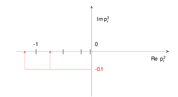
Figure 4: Paths followed in the complex $p_{r}^{2}$ plane. On the real axis are indicated the positions of the threshold (-1) and pseudo-thresholds.

The execution of the program is rather fast and precise: with an Intel Pentium III of 1 GHz we get values with 7 digits requiring times ranging from a fraction of a second to 10 seconds of CPU, and with 11 digits from few tens of seconds to one hour.

If $\Delta=L/N$ is the length of one step, $L$ is the length of the whole path and $N$ the total number of steps, the 4th-order Runge-Kutta formula discards terms of order $\Delta^{5}$, so the whole error behaves as $\epsilon_{RK}=N\Delta^{5}=L^{5}/N^{4}$, and a proper choice of $L$ and $N$ allows the control of the precision.

Indeed we estimate the relative error, as usual, by comparing a value obtained with $N$ steps with the one obtained with $N/10$ steps, $\epsilon_{RK}=[V(N)-V(N/10)]/V(N)$, to which we add a cumulative rounding error $\epsilon_{cre}=\sqrt{N}\times 10^{-15}$, due to our 15 digits double precision FORTRAN implementation.

The general massive sunrise graph is numerically well studied in literature and several numerical methods are developed, such as multiple expansions [12], or numerical integration [12, 13, 14, 15, 16, 17]. Comparisons are presented in [6] with some values available in the literature [12, 17] with excellent agreement (up to more than 11 digits).

5 Perspectives

The presented method for numerically advancing the solutions of the MDE is rather precise and competitive with other available methods for numerical MI calculations.

Rather than conclusions it is more appropriate at this stage to present perspectives. It seems to be possible to complete the 2-loop self-mass for arbitrary internal masses and we have almost completed the 4-denominators case [9].

We think that the extension to graphs with more loops or legs do not present serious problems, even if the growth in the number of MI increases the computing time.

It is worth to mention that the method relies on the same MDE, which are used also for analytic calculations, so it provides a ’low-cost’ comforting cross-check for those results.

References

• [1] F.V. Tkachov, Phys. Lett.B 100, 65 (1981); K.G. Chetyrkin and F.V. Tkachov, Nucl. Phys.B 192, 159 (1981).
• [2] A.V. Kotikov, Phys. Lett.B254, 158 (1991).
• [3] E. Remiddi, Nuovo Cim.A110, 1435 (1997), hep-th/9711188.
• [4] W.H.Press, S.A. Teukolsky, W.T. Vetterling and B.P. Flannery, Numerical Recipes in FORTRAN. The art of Scientific Computing, Cambridge Univ. Press, 1994.
• [5] M. Caffo, H. Czyż, S. Laporta and E. Remiddi, Nuovo Cim.A 111, 365 (1998), hep-th/9805118.
• [6] M. Caffo, H. Czyż and E. Remiddi, Nucl. Phys.B 634, 309 (2002), hep-ph/0203256.
• [7] O.V. Tarasov, Nucl. Phys.B 502, 455 (1997), hep-ph/9703319.
• [8] M. Caffo, H. Czyż, S. Laporta and E. Remiddi, Acta Phys. Pol.B 29, 2627 (1998), hep-th/9807119.
• [9] M. Caffo, H. Czyż, A. Grzeliṅska and E. Remiddi, in preparation.
• [10] M. Caffo, H. Czyż and E. Remiddi, Nucl. Phys.B 581, 274 (2000), hep-ph/9912501.
• [11] M. Caffo, H. Czyż and E. Remiddi, Nucl. Phys.B 611, 503 (2001), hep-ph/0103014.
• [12] F.A. Berends, M. Böhm, M. Buza and R. Scharf, Z. Phys.C 63, 227 (1994).
• [13] S. Bauberger, F.A. Berends, M. Böhm and M. Buza, Nucl. Phys.B 434, 383 (1995).
• [14] A. Ghinculov and J.J. van der Bij, Nucl. Phys.B 436, 30 (1995).
• [15] P. Post and J.B. Tausk, Mod. Phys. Lett.A 11, 2115 (1996), hep-ph/9604270.
• [16] S. Groote, J.G. Körner and A.A. Pivovarov, Eur. Phys. J.C 11, 279 (1999), hep-ph/9903412; Nucl. Phys.B 542, 515 (1999), hep-ph/9806402.
• [17] G. Passarino, Nucl. Phys.B 619, 257 (2001), hep-ph/0108252.