$\bm{CP}$ Violation in Hyperon Nonleptonic Decays
within the Standard Model

Abstract

We calculate the $CP$-violating asymmetries $A(\Lambda^{0}_{-})$ and $A(\Xi^{-}_{-})$ in nonleptonic hyperon decay within the Standard Model using the framework of heavy-baryon chiral perturbation theory ($\chi$PT). We identify those terms that correspond to previous calculations and discover several errors in the existing literature. We present a new result for the lowest-order (in $\chi$PT) contribution of the penguin operator to these asymmetries, as well as an estimate for the uncertainty of our result that is based on the calculation of the leading nonanalytic corrections.

I Introduction

In nonleptonic hyperon decays such as $\,\Lambda\to p\pi^{-},\,$ it is possible to search for $CP$ violation by comparing the angular distribution with that of the corresponding anti-hyperon decay op . The Fermilab experiment HyperCP is currently analyzing data searching for $CP$ violation in such a decay.

The reaction of interest for HyperCP is the decay of a polarized $\Lambda$, with known polarization $\bm{w}$, into a proton (whose polarization is not measured) and a $\pi^{-}$ with momentum $\bm{q}$. The interesting observable is a correlation in the decay distribution of the form

$$\frac{{\rm d}\Gamma}{{\rm d}\Omega}\,\sim\,1+\alpha\,\bm{w}\cdot\bm{q}\,\,.$$ (1)

The branching ratio for this mode is $63.9\%$, and the parameter $\alpha$ has been measured to be $\,\alpha_{\Lambda}=0.642\,$ pdb . The $CP$ violation in question involves a comparison of the parameter $\alpha$ with the corresponding parameter $\bar{\alpha}$ from the reaction $\,\bar{\Lambda}\to\bar{p}\pi^{+}.\,$

To obtain polarized $\Lambda$’s with known polarization, it is necessary to study the double decay chain $\,\Xi^{-}\to\Lambda\pi^{-}\to p\pi^{-}\pi^{-}\,$ e756 ; hypercp . This eventually leads to the experimental observable being sensitive to the sum of $CP$ violation in the $\Xi$ decay and $CP$ violation in the $\Lambda$ decay.

In both reactions, $\,\Xi^{-}\to\Lambda\pi^{-}\,$ and $\,\Lambda\to p\pi^{-},\,$ the final state can be reached from the initial state via $\,|\Delta I|=\frac{1}{2}\,$ or $\,|\Delta I|=\frac{3}{2}\,$ transitions. It is known that due to the existence of a strong $\,|\Delta I|=\frac{1}{2}\,$ rule for nonleptonic hyperon decay, the dominant contribution to the $CP$-violating asymmetries arises from interference between an $S$-wave and a $P$-wave within the $\,|\Delta I|=\frac{1}{2}\,$ transition dp ; dhp ; hsv . One can define the $CP$-violating asymmetries

$$A_{\Lambda}\,\equiv\,A\bigl{(}\Lambda^{0}_{-}\bigr{)}\,\equiv\,\frac{\alpha_{\Lambda}-\bar{\alpha}_{\Lambda}}{\alpha_{\Lambda}+\bar{\alpha}_{\Lambda}}\,\,,\hskip 30.00005ptA_{\Xi}\,\equiv\,A\bigl{(}\Xi^{-}_{-}\bigr{)}\,\equiv\,\frac{\alpha_{\Xi}-\bar{\alpha}_{\Xi}}{\alpha_{\Xi}+\bar{\alpha}_{\Xi}}$$ (2)

for the $\Lambda$ and $\Xi^{-}$ decays, respectively. The experimental observable is then e756 ; hypercp

$$A_{\Xi\Lambda}\,\simeq\,A_{\Lambda}+A_{\Xi}\,\,.$$ (3)

Approximate expressions have been obtained for $A_{\Lambda,\Xi}$ in the case of $\,|\Delta I|=\frac{1}{2}\,$ dominance dhp , namely

$$\begin{array}[]{c}\displaystyle A_{\Lambda}\,\simeq\,-\tan\left(\delta_{P}^{\Lambda}-\delta_{S}^{\Lambda}\right)\sin\left(\phi_{P}^{\Lambda}-\phi_{S}^{\Lambda}\right)\,\,,\vspace{2ex}\\ \displaystyle A_{\Xi}\,\simeq\,-\tan\left(\delta_{P}^{\Xi}-\delta_{S}^{\Xi}\right)\sin\left(\phi_{P}^{\Xi}-\phi_{S}^{\Xi}\right)\,\,.\end{array}$$ (4)

Here, $\delta_{S}^{\Lambda}$ $\bigl{(}\delta_{P}^{\Lambda}\bigr{)}$ is the strong $S$-wave ($P$-wave) $N\pi$ scattering phase-shift at $\,\sqrt{s}=M_{\Lambda},\,$ and $\delta_{S}^{\Xi}$ $\bigl{(}\delta_{P}^{\Xi}\bigr{)}$ is the strong $S$-wave ($P$-wave) $\Lambda\pi$ scattering phase-shift at $\,\sqrt{s}=M_{\Xi}.\,$ Moreover, $\phi_{S}^{\Lambda,\Xi}$ $\bigl{(}\phi_{P}^{\Lambda,\Xi}\bigr{)}$ are the $CP$-violating weak phases induced by the $\,|\Delta S|=1,\,$ $|\Delta I|=\frac{1}{2}\,$ interaction in the $S$-wave ($P$-wave) of the $\,\Lambda\to p\pi^{-}\,$ and $\,\Xi^{-}\to\Lambda\pi^{-}\,$ decays, respectively.

Experimentally, the current published limit is $\,A_{\Xi\Lambda}=0.012\pm 0.014\,$ from E756 e756 , and the expected sensitivity of HyperCP is $10^{-4}\,$ hypercp . In addition, HyperCP has recently obtained a preliminary measurement of $\,A_{\Xi\Lambda}=(-7\pm 12\pm 6.2)\times 10^{-4}\,$ zyla . Previous estimates for $A_{\Xi\Lambda}$ indicated that it occurs at the few times $10^{-5}$ level within the standard model dhp ; hsv ; im and that it can be as large as $10^{-3}$ beyond the standard model dhp ; NP . The larger asymmetries occur in models with an enhanced gluon-dipole operator that is parity-even and thus does not contribute to the $\epsilon^{\prime}$ parameter in kaon decay. The $10^{-3}$ upper bound corresponds to the phenomenological constraint from new contributions to the $\epsilon$ parameter in kaon mixing. This illustrates the relevance of the HyperCP measurement which complements the $\epsilon^{\prime}$ experiments in the study of $CP$ violation in $\,|\Delta S|=1\,$ transitions.

The strong $\pi N$ scattering phases needed in Eq. (4) have been measured to be $\,\delta_{S}^{\Lambda}\sim 6^{\circ}\,$ and $\,\delta_{P}^{\Lambda}\sim-1^{\circ}\,$ with errors of about $1^{\circ}\,$ roper . In contrast, the strong $\Lambda\pi$ scattering phases have not been measured. Modern calculations based on chiral perturbation theory indicate that these phases are small, with $\bigl{|}\delta_{S}^{\Xi}\bigr{|}$ being at most $7^{\circ}\,$ lsw ; DatPak ; kamal ; ttv ; mo ; kaiser . For our numerical estimates, we will allow the $\Lambda\pi$ phases to vary within the range obtained at next-to-leading order in heavy-baryon chiral perturbation theory ttv ,

$$\begin{array}[]{c}\displaystyle-3.0^{\circ}\,\leq\,\delta_{S}^{\Xi}\,\leq\,+0.4^{\circ}\,\,,\hskip 30.00005pt-3.5^{\circ}\,\leq\,\delta_{P}^{\Xi}\,\leq\,-1.2^{\circ}\,\,.\end{array}$$ (6)

One could choose to be less constrained and include the larger $\,\delta_{S}^{\Xi}=-7^{\circ}\,$ found in Ref. ttv , but this would only enlarge the $\delta_{S}^{\Xi}$ range and hence the uncertainty of the predicted asymmetry. In any case, eventually these phases can be extracted directly from the measurement of the decay distribution in $\,\Xi\to\Lambda\pi\,$ hypercp ; alak ; huang . Recently E756 has reported a preliminary result of $\,\delta_{P}^{\Xi}-\delta_{S}^{\Xi}=3.17^{\circ}\pm 5.45^{\circ}\,$ alak .

In this paper, we estimate the weak phases that appear in $A_{\Lambda}$ and $A_{\Xi}$ within the standard model. In Sec. II, we present a calculation of the weak phases guided by heavy-baryon chiral perturbation theory in terms of three unknown weak counterterms. In Sec. III, we estimate the value of these counterterms by considering contributions that arise from the factorization of the penguin operator and also nonfactorizable contributions estimated in the MIT bag model. Sec. IV contains the resulting weak phases and $CP$-violating asymmetries. Finally, in Sec. V, we compare our results to those of previous work and present our conclusions. For completeness, we also provide in an appendix the results for the corresponding asymmetries in $\,\Sigma\to N\pi\,$ decays.

II Chiral perturbation theory

The chiral Lagrangian that describes the interactions of the lowest-lying mesons and baryons is written down in terms of the lightest meson-octet, baryon-octet, and baryon-decuplet fields bsw ; georgi ; dgh ; JenMan1 . The meson and baryon octets are collected into $3\times 3$ matrices $\varphi$ and $B$, respectively, and the decuplet fields are represented by the Rarita-Schwinger tensor $T_{abc}^{\mu}$, which is completely symmetric in its SU(3) indices ($a,b,c$). The octet mesons enter through the exponential $\,\Sigma=\xi^{2}=\exp({\rm i}\varphi/f),\,$ where $f$ is the pion-decay constant.

In the heavy-baryon formalism JenMan1 ; JenMan2 , the baryons in the chiral Lagrangian are described by velocity-dependent fields, $B_{v}$ and $T_{v}^{\mu}$. For the strong interactions, the leading-order Lagrangian is given by JenMan1 ; JenMan2 ; JenMan3

$${\cal L}_{\rm s}^{(1)} = \mbox{$\frac{1}{4}$}f^{2}\left\langle\partial^{\mu}\Sigma^{\dagger}\,\partial_{\mu}\Sigma\right\rangle+\left\langle\bar{B}_{v}\,{\rm i}v\cdot{\cal D}B_{v}\right\rangle+2D\left\langle\bar{B}_{v}S_{v}^{\mu}\left\{{\cal A}_{\mu},B_{v}\right\}\right\rangle+2F\left\langle\bar{B}_{v}S_{v}^{\mu}\left[{\cal A}_{\mu},B_{v}\right]\right\rangle$$ (7)

$$-\,\,\bar{T}_{v}^{\mu}{\rm i}v\cdot{\cal D}T_{v\mu}+\Delta m\,\bar{T}_{v}^{\mu}T_{v\mu}+{\cal C}\left(\bar{T}_{v}^{\mu}{\cal A}_{\mu}B_{v}+\bar{B}_{v}{\cal A}_{\mu}T_{v}^{\mu}\right)+2{\cal H}\,\bar{T}_{v}^{\mu}S_{v}\cdot{\cal A}T_{v\mu}\,\,,$$

where $\langle\cdots\rangle$ denotes ${\rm Tr}(\cdots)$ in flavor-SU(3) space, $S_{v}$ is the spin operator, and

$$\begin{array}[]{c}\displaystyle{\cal A}_{\mu}\,=\,\mbox{$\frac{\rm i}{2}$}\left(\xi\,\partial_{\mu}\xi^{\dagger}-\xi^{\dagger}\,\partial_{\mu}\xi\right)\,=\,\frac{\partial_{\mu}\varphi}{2f}\,\,+\,\,{\cal O}(\varphi^{3})\,\,,\end{array}$$ (9)

with further details given in Ref. atv . In this Lagrangian, $D$, $F$, $\cal C$, and $\cal H$ are free parameters, which can be determined from hyperon semileptonic decays and from strong decays of the form $\,T\to B\phi.\,$ Fitting tree-level formulas, one extracts JenMan1 ; JenMan2

$$\begin{array}[]{c}\displaystyle D\,=\,0.80\,\,,\hskip 30.00005ptF\,=\,0.50\,\,,\hskip 30.00005pt|{\cal C}|\,=\,1.7\,\,,\end{array}$$ (11)

whereas $\cal H$ is undetermined from this fit. From the nonrelativistic quark models, one finds the relations JenMan3

$$\begin{array}[]{c}\displaystyle 3F\,=\,2D\,\,,\hskip 20.00003pt{\cal C}\,=\,-2D\,\,,\hskip 20.00003pt{\cal H}\,=\,-3D\,\,,\end{array}$$ (13)

which are well satisfied by $D$, $F$, and $\cal C$, suggesting the tree-level value

$${\cal H}\,=\,-2.4\,\,.$$ (14)

In our numerical estimates, we use Eqs. (11) and (14) for the leading-order results and the estimate of their uncertainty from one-loop contributions, with $\cal C$ and $\cal H$ only appearing in loop diagrams involving decuplet baryons. As another estimate of the uncertainty in these results, we will evaluate the effect of varying $D$ and $F$ between their tree-level values above and their one-loop values to be given later.

At next-to-leading order, the strong Lagrangian contains a greater number of terms L2refs . The ones of interest here are those that explicitly break chiral symmetry, containing one power of the quark-mass matrix $\,M={\rm diag}\bigl{(}0,0,m_{s}\bigr{)}.\,$ For our calculation of the factorization of the penguin operator, we will need these terms in the form

$${\cal L}_{\rm s}^{(2)} = \mbox{$\frac{1}{4}$}f^{2}\left\langle\chi_{+}\right\rangle+\frac{b_{D}}{2B_{0}}\left\langle\bar{B}_{v}\left\{\chi_{+},B_{v}\right\}\right\rangle+\frac{b_{F}}{2B_{0}}\left\langle\bar{B}_{v}\left[\chi_{+},B_{v}\right]\right\rangle+\frac{b_{0}}{2B_{0}}\left\langle\chi_{+}\right\rangle\left\langle\bar{B}_{v}B_{v}\right\rangle$$ (15)

$$+\,\,\frac{c}{2B_{0}}\,\bar{T}_{v}^{\mu}\chi_{+}T_{v\mu}-\frac{c_{0}}{2B_{0}}\left\langle\chi_{+}\right\rangle\bar{T}_{v}^{\mu}T_{v\mu}\,\,,$$

where we have used the notation $\,\chi_{+}=\xi^{\dagger}\chi\xi^{\dagger}+\xi\chi^{\dagger}\xi\,$ to introduce coupling to external (pseudo)scalar sources, $\,\chi=s+ip,\,$ such that in the absence of the external sources $\chi$ reduces to the mass matrix, $\,\chi=2B_{0}M.\,$ As will be discussed in the next section, we also need from the meson sector the next-to-leading-order Lagrangian

$${\cal L}_{\rm s}^{(4)}\,=\,L_{5}\left\langle\partial^{\mu}\Sigma^{\dagger}\,\partial_{\mu}\Sigma\,\xi^{\dagger}\chi_{+}\xi\right\rangle\,\,+\,\,\cdots\,\,,$$ (16)

where only the relevant term is explicitly shown. In Eqs. (15) and (16), the constants $B_{0}$, $b_{D,F,0}$, $c$, $c_{0}$, and $L_{5}$ are free parameters to be fixed from data.

As is well known, the weak interactions responsible for hyperon nonleptonic decays are described by a $\,|\Delta S|=1\,$ Hamiltonian that transforms as $\bigl{(}8_{\rm L},1_{\rm R}\bigr{)}\oplus\bigl{(}27_{\rm L},1_{\rm R}\bigr{)}$ under SU(3$)_{\rm L}$$\times$SU(3$)_{\rm R}$ rotations. It is also known from experiment that the octet term dominates the 27-plet term, as indicated by the fact that the $\,|\Delta I|=\frac{1}{2}\,$ components of the decay amplitudes are larger than the $\,|\Delta I|=\frac{3}{2}\,$ components by about twenty times atv ; over . We shall, therefore, assume in what follows that the decays are completely characterized by the $(8_{\rm L},1_{\rm R})$, $\,|\Delta I|=\frac{1}{2}\,$ interactions. The leading-order chiral Lagrangian for such interactions is bsw ; jenkins2

$${\cal L}_{\rm w} = h_{D}\left\langle\bar{B}_{v}\left\{\xi^{\dagger}h\xi\,,\,B_{v}\right\}\right\rangle+h_{F}\left\langle\bar{B}_{v}\left[\xi^{\dagger}h\xi\,,\,B_{v}\right]\right\rangle+h_{C}\,\bar{T}_{v}^{\mu}\,\xi^{\dagger}h\xi\,T_{v\mu}$$ (17)

$$+\,\,\gamma_{8}f^{2}\left\langle h\,\partial_{\mu}\Sigma\,\partial^{\mu}\Sigma^{\dagger}\right\rangle\,\,+\,\,{\rm H.c.}\,\,,$$

where $h$ is a 3$\times$3 matrix with elements $\,h_{ij}=\delta_{i2}\delta_{3j},\,$ and the parameters $h_{D,F,C}$ and $\gamma_{8}$ contain the weak phases to be discussed below.

The weak Lagrangian in Eq. (17) is thus the leading-order (in $\chi$PT) realization of the effective $\,|\Delta S|=1\,$ Hamiltonian in the standard model buras ,

$${\cal H}_{\rm w}\,=\,\frac{G_{\rm F}}{\sqrt{2}}\,V_{ud}^{*}V_{us}\,\sum_{i=1}^{10}C_{i}\,Q_{i}\,\,+\,\,{\rm H.c}\,\,,$$ (18)

where $G_{\rm F}$ is the Fermi coupling constant, $V_{kl}$ are the elements of the Cabibbo-Kobayashi-Maskawa (CKM) matrix ckm ,

$$C_{i}\,\equiv\,z_{i}+\tau y_{i}\,\equiv\,z_{i}\,-\,\frac{V_{td}^{*}V_{ts}}{V_{ud}^{*}V_{us}}\,\,y_{i}$$ (19)

are the Wilson coefficients, and $Q_{i}$ are four-quark operators whose expressions can be found in Ref. buras . Later on, we will express $V_{kl}$ in the Wolfenstein parametrization wolfenstein . It follows that

$$V_{ud}^{*}V_{us}\,=\,\lambda\,\,,\hskip 30.00005ptV_{td}^{*}V_{ts}\,=\,-\lambda^{5}A^{2}\,(1-\rho+{\rm i}\eta)$$ (20)

at lowest order in $\lambda$. For our numerical estimates, the relevant parameters that we will employ are ckmfit

$$\lambda\,=\,0.2219\,\,,\hskip 20.00003ptA\,=\,0.832\,\,,\hskip 20.00003pt\eta\,=\,0.339\,\,.$$ (21)

In the next section, we match the penguin operator $Q_{6}$ in the short-distance Hamiltonian of Eq. (18) with the corresponding Lagrangian parameters in Eq. (17).

We now have all the ingredients necessary to calculate the weak decay amplitudes in terms of the four parameters $h_{D,F,C}$ and $\gamma_{8}$ (only the first two are needed at leading order). In the heavy-baryon formalism, the amplitude for the weak decay of a spin-$\frac{1}{2}$ baryon $B$ into another spin-$\frac{1}{2}$ baryon $B^{\prime}$ and a pseudoscalar meson $\phi$ has the general form jenkins2

$${\rm i}{\cal M}_{B\to B^{\prime}\phi}\,=\,-{\rm i}\bigl{\langle}B^{\prime}\phi\bigr{|}{\cal L}_{\rm w+s}\bigl{|}B\bigr{\rangle}\,=\,\bar{u}_{B^{\prime}}\,\Bigl{(}{\cal A}_{BB^{\prime}\phi}^{(S)}+2S_{v}\!\cdot\!p_{\phi}\,{\cal A}_{BB^{\prime}\phi}^{(P)}\Bigr{)}\,u_{B}\,\,,$$ (22)

where the superscripts refer to the $S$- and $P$-wave components of the amplitude. To express our results, we also adopt the notation jenkins2

$${a}^{(S,P)}_{BB^{\prime}\phi}\,\equiv\,\sqrt{2}\,f\,{\cal A}^{(S,P)}_{BB^{\prime}\phi}\,\,.$$ (23)

With the Lagrangians given above, one can derive the amplitudes at leading order, represented by the diagrams in Fig. 1. Fig. 1(a) indicates that the $S$-wave is directly obtained from a weak vertex provided by Eq. (17). The leading contribution to the $P$-wave arises from baryon-pole diagrams, as in Fig. 1(b), which each involve a weak vertex from Eq. (17) and a strong vertex from Eq. (7). Thus the leading-order results for amplitudes not related by isospin are bsw ; jenkins2

$$\begin{array}[]{c}\displaystyle{a}^{(S)}_{\Lambda p\pi^{-}}\,=\,\mbox{$\frac{1}{\sqrt{6}}$}\bigl{(}h_{D}+3h_{F}\bigr{)}\,\,,\hskip 20.00003pt{a}^{(S)}_{\Xi^{-}\Lambda\pi^{-}}\,=\,\mbox{$\frac{1}{\sqrt{6}}$}\bigl{(}h_{D}-3h_{F}\bigr{)}\,\,,\vspace{2ex}\\ \displaystyle{a}^{(S)}_{\Sigma^{+}n\pi^{+}}=0\,\,,\hskip 20.00003pt{a}^{(S)}_{\Sigma^{-}n\pi^{-}}=-h_{D}+h_{F}\,\,,\end{array}$$ (24c)

$$\begin{array}[]{c}\displaystyle{a}^{(P)}_{\Lambda p\pi^{-}}\,=\,\displaystyle\frac{2D\,\bigl{(}h_{D}-h_{F}\bigr{)}}{\sqrt{6}\,\,\bigl{(}m_{\Sigma}-m_{N}\bigr{)}}+\frac{(D+F)\,\bigl{(}h_{D}+3h_{F}\bigr{)}}{\sqrt{6}\,\,\bigl{(}m_{\Lambda}-m_{N}\bigr{)}}\,\,,\vspace{2ex}\\ \displaystyle{a}^{(P)}_{\Xi^{-}\Lambda\pi^{-}}\,=\,\displaystyle\frac{-2D\,\bigl{(}h_{D}+h_{F}\bigr{)}}{\sqrt{6}\,\,\bigl{(}m_{\Xi}-m_{\Sigma}\bigr{)}}-\frac{(D-F)\,\bigl{(}h_{D}-3h_{F}\bigr{)}}{\sqrt{6}\,\,\bigl{(}m_{\Xi}-m_{\Lambda}\bigr{)}}\,\,,\vspace{2ex}\\ \displaystyle{a}^{(P)}_{\Sigma^{+}n\pi^{+}}\,=\,\displaystyle\frac{-D\,\bigl{(}h_{D}-h_{F}\bigr{)}}{m_{\Sigma}-m_{N}}-\frac{\mbox{$\frac{1}{3}$}D\,\bigl{(}h_{D}+3h_{F}\bigr{)}}{m_{\Lambda}-m_{N}}\,\,,\vspace{2ex}\\ \displaystyle{a}^{(P)}_{\Sigma^{-}n\pi^{-}}\,=\,\displaystyle\frac{-F\,\bigl{(}h_{D}-h_{F}\bigr{)}}{m_{\Sigma}-m_{N}}-\frac{\mbox{$\frac{1}{3}$}D\,\bigl{(}h_{D}+3h_{F}\bigr{)}}{m_{\Lambda}-m_{N}}\,\,.\end{array}$$ (24h)

The leading nonanalytic contributions to the amplitudes arise from one-loop diagrams, with $h_{C}$ only appearing in those involving decuplet baryons. These contributions have been calculated by various authors bsw ; jenkins2 ; nlhd ; at , and we will adopt the results of Ref. at for the numerical estimate of our uncertainty.

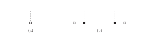
Figure 1: Leading-order diagrams for (a) $S$-wave and (b) $P$-wave hyperon nonleptonic decays. In all figures, a solid (dashed) line denotes a baryon-octet (meson-octet) field, and a solid dot (hollow square) represents a strong (weak) vertex, with the strong vertices being generated by ${\cal L}_{\rm s}^{(1)}$ in Eq. (7). Here the weak vertices come from the $h_{D,F}$ terms in Eq. (17).

In Fig. 2, we show the kaon-pole diagram to be discussed later on. In this diagram, there is a strong vertex from Eq. (7) followed by a kaon pole and a weak vertex from the $\gamma_{8}$ term in Eq. (17). Notice that this term is not only subleading in the chiral expansion, but also suppressed by an $m_{\pi}^{2}/m_{K}^{2}$ factor (and hence vanishing in the $\,m_{u}=m_{d}=0\,$ limit).

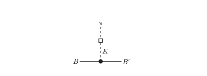
Figure 2: Kaon-pole diagram contributing to $P$-wave hyperon nonleptonic decays. The weak vertex here comes from the $\gamma_{8}$ term in Eq. (17)

Once the values of the weak couplings $h_{D,F}$ are specified, the formulas in Eq. (24) determine the leading-order amplitudes. It is well known that this representation does not provide a good fit to the measured $P$-wave amplitudes, and that higher-order terms are important bsw ; dgh ; jenkins2 ; nlhd ; at ; BorHol . The procedure that we adopt for estimating the weak phases is to obtain the real part of the amplitudes from experiment (assuming no $CP$ violation) and to use Eq. (24) to estimate the imaginary parts. The dominant $CP$-violating phases in the $\,|\Delta I|=\frac{1}{2}\,$ sector of the $\,|\Delta S|=1\,$ weak interaction occur in the Wilson coefficient $C_{6}$ associated with the penguin operator $Q_{6}$. Our strategy will be to calculate within a model the imaginary part of the couplings $h_{D,F,C}$ and $\gamma_{8}$ induced by $Q_{6}$. As a numerical result, we propose a central value from leading-order $\chi$PT [Eq. (24)] and an estimate of the error from the nonanalytic corrections obtained with the expressions given in Ref. at .

To end this section, for later use we collect in Table 1 the experimental values of the $S$- and $P$-wave amplitudes of interest, reproduced from Ref. at . The numbers are extracted (neglecting strong and weak phases) from the measured decay width $\Gamma$ and decay parameter $\alpha$ by means of the relations

$$\begin{array}[]{c}\displaystyle\Gamma\,=\,\frac{\bigl{|}\mbox{$\bm{p}$}_{B^{\prime}}\bigr{|}}{4\pi\,m_{B}}\bigl{(}E_{B^{\prime}}+m_{B^{\prime}}\bigr{)}\left(|s|^{2}+|p|^{2}\right)\,\,,\hskip 30.00005pt\alpha\,=\,\frac{2\,{\rm Re}(s^{*}p)}{|s|^{2}+|p|^{2}}\,\,.\end{array}$$ (26)

The $s$ and $p$ amplitudes are related to those in Eq. (22) above by

$$s\,=\,{\cal A}^{(S)}\,\,,\hskip 30.00005ptp\,=\,\bigl{|}\mbox{$\bm{p}$}_{B^{\prime}}\bigr{|}\,{\cal A}^{(P)}\,\,.$$ (27)

Table 1: Experimental values for $S$- and $P$-wave amplitudes, in units of $G_{\rm F}m_{\pi^{+}}^{2}$.

Decay mode	$\hskip 3.44444pts$	$\hskip 3.44444ptp$
$\begin{array}[]{rcl}\displaystyle\Lambda&\to&p\pi^{-}\\ \Xi^{-}&\to&\Lambda\pi^{-}\\ \Sigma^{+}&\to&n\pi^{+}\\ \Sigma^{+}&\to&p\pi^{0}\\ \Sigma^{-}&\to&n\pi^{-}\end{array}$	$\begin{array}[]{rcl}\displaystyle 1.42&\pm&0.01\\ -1.98&\pm&0.01\\ 0.06&\pm&0.01\\ -1.43&\pm&0.05\\ 1.88&\pm&0.01\end{array}$	$\begin{array}[]{rcl}\displaystyle 0.52&\pm&0.01\\ 0.48&\pm&0.02\\ 1.81&\pm&0.01\\ 1.17&\pm&0.06\\ -0.06&\pm&0.01\end{array}$

III Estimate of counterterms

Our task in this section is to match the dominant $\,|\Delta I|=\frac{1}{2}\,$ $CP$-violating term from the standard-model effective weak Hamiltonian in Eq. (18) to the weak chiral Lagrangian in Eq. (17). That is, to compute the imaginary part of the parameters $h_{D}$, $h_{F}$, $h_{C}$, and $\gamma_{8}$ that is induced by $\,{\rm Im}\,C_{6}Q_{6}\,$ in Eq. (18). To do this, we will include both factorizable contributions, that arise from regarding the operator $Q_{6}$ as the product of two (pseudo)scalar densities, and direct (nonfactorizable) contributions calculated in the MIT bag model.

The nonfactorizable contributions are easily obtained from the observation that the weak chiral Lagrangian of Eq. (17) is responsible for nondiagonal “weak mass terms” such as

$$\begin{array}[]{c}\displaystyle\bigl{\langle}n\bigr{|}\bigl{(}{\cal H}_{\rm w}\bigr{)}_{8}\bigl{|}\Lambda\bigr{\rangle}\,=\,\frac{h_{D}+3h_{F}}{\sqrt{6}}\,\bar{u}_{n}u_{\Lambda}\,\,,\vspace{2ex}\\ \displaystyle\bigl{\langle}\Lambda\bigr{|}\bigl{(}{\cal H}_{\rm w}\bigr{)}_{8}\bigl{|}\Xi^{0}\bigr{\rangle}\,=\,\frac{h_{D}-3h_{F}}{\sqrt{6}}\,\bar{u}_{\Lambda}u_{\Xi}\,\,,\vspace{2ex}\\ \displaystyle\bigl{\langle}\Xi^{*-}\bigr{|}\bigl{(}{\cal H}_{\rm w}\bigr{)}_{8}\bigl{|}\Omega^{-}\bigr{\rangle}\,=\,\frac{-h_{C}}{\sqrt{3}}\,\bar{u}_{\Xi^{*}}\cdot u_{\Omega}\,\,,\end{array}$$ (31)

where the subscript 8 denotes the component of ${\cal H}_{\rm w}$ that transforms as $(8_{\rm L},1_{\rm R})$. These terms can be computed directly from the short-distance Hamiltonian in Eq. (18) by calculating in the MIT bag model the baryon-baryon matrix elements of the four-quark operators. From the basic results in Appendix A, one finds the $Q_{6}$ contributions

$$\begin{array}[]{c}\displaystyle h_{D}\,=\,\frac{G_{\rm F}\lambda}{\sqrt{2}}\,C_{6}\,(3\,a-5\,b)\,\,,\hskip 20.00003pth_{F}\,=\,\frac{G_{\rm F}\lambda}{\sqrt{2}}\,C_{6}\,\Bigl{(}a+\mbox{$\frac{11}{3}$}\,b\Bigr{)}\,\,,\vspace{2ex}\\ \displaystyle h_{C}\,=\,\frac{G_{\rm F}\lambda}{\sqrt{2}}\,C_{6}\,(-12\,a+4\,b)\,\,,\end{array}$$ (34)

where $a$ and $b$ are bag parameters whose values are given in Eq. (85) for $h_{D,F}$ and in Eq. (86) for $h_{C}$. Numerically, the imaginary part of $C_{6}$ then yields, in units of $\,\sqrt{2}\,f_{\pi}G_{\rm F}m_{\pi^{+}}^{2}\,\lambda^{5}A^{2}\eta,\,$

$$\begin{array}[]{c}\displaystyle{\rm Im}\,h_{D}\,=\,0.278\,\,y_{6}\,\,,\hskip 20.00003pt{\rm Im}\,h_{F}\,=\,1.04\,\,y_{6}\,\,,\hskip 20.00003pt{\rm Im}\,h_{C}\,=\,-3.13\,\,y_{6}\,\,,\end{array}$$ (36)

where $\,f_{\pi}\simeq 92.4\,\rm MeV\,$ has been used. The units are chosen to separate both the conventional normalization for the hyperon decay amplitudes, as in Eq. (23) and Table 1, and the relevant combination of CKM parameters occurring in the observables $A_{\Lambda,\Xi}$.

To obtain the factorizable contributions to the imaginary part of the parameters $h_{D,F,C}$, we follow the procedure used in kaon physics for $\gamma_{8}\,$ penfac . As shown in Appendix B, the lowest-order chiral realization of a factorized $Q_{6}$ contributes to the weak Lagrangian in Eq. (17) with

$$\begin{array}[]{c}\displaystyle h_{D}\,=\,\frac{G_{\rm F}\,\lambda}{\sqrt{2}}\,\,8\,C_{6}\,f^{2}B_{0}\,b_{D}\,\,,\hskip 30.00005pth_{F}\,=\,\frac{G_{\rm F}\,\lambda}{\sqrt{2}}\,\,8\,C_{6}\,f^{2}B_{0}\,b_{F}\,\,,\vspace{2ex}\\ \displaystyle h_{C}\,=\,\frac{G_{\rm F}\,\lambda}{\sqrt{2}}\,\,8\,C_{6}\,f^{2}B_{0}\,c\,\,,\hskip 30.00005pt\gamma_{8}\,=\,\frac{G_{\rm F}\,\lambda}{\sqrt{2}}\,\,16\,C_{6}\,B_{0}^{2}\,L_{5}\,\,.\end{array}$$ (39)

The values of $b_{D}$, $b_{F}$, and $c$ can be determined by fitting the mass formulas derived from the Lagrangian in Eq. (15), with $\chi=2B_{0}M,\,$ to the measured masses of the octet and decuplet baryons pdb . Thus we find

$$b_{D}\,m_{s}\,=\,0.0301\,\,{\rm GeV}\,\,,\hskip 20.00003ptb_{F}\,m_{s}\,=\,-0.0948\,\,{\rm GeV}\,\,,\hskip 20.00003ptc\,m_{s}\,=\,0.221\,\,{\rm GeV}\,\,$$ (40)

for $\,m_{u}=m_{d}=0.\,$ In this limit, the Lagrangian in Eq. (15) also gives $\,m_{K}^{2}=B_{0}\,m_{s}.\,$ Using $\,m_{s}=\bar{m}_{s}(\mu=m_{c})=170\,\rm MeV\,$ from Ref. buras , we then have

$$b_{D}\,=\,0.177\,\,,\hskip 20.00003ptb_{F}\,=\,-0.558\,\,,\hskip 20.00003ptc\,=\,1.30\,\,,\hskip 20.00003ptB_{0}\,=\,1.45~{}{\rm GeV}\,\,.$$ (41)

For $L_{5}$, we adopt the value $\,L_{5}=1.4\times 10^{-3}\,$ found in Ref. gl . Setting $\,f=f_{\pi}\simeq 92.4\,\rm MeV,\,$ we then obtain the $Q_{6}$ contributions, in units of $\,\sqrt{2}\,f_{\pi}G_{\rm F}m_{\pi^{+}}^{2}\,\eta\lambda^{5}A^{2},\,$

$$\begin{array}[]{c}\displaystyle{\rm Im}\,h_{D}\,=\,4.86\,y_{6}\,\,,\hskip 30.00005pt{\rm Im}\,h_{F}\,=\,-15.3\,y_{6}\,\,,\hskip 30.00005pt{\rm Im}\,h_{C}\,=\,35.6\,y_{6}\,\,,\vspace{2ex}\\ \displaystyle{\rm Im}\,\gamma_{8}\;B_{0}\,=\,18.8\,y_{6}B_{6}^{(1/2)}\,\,,\end{array}$$ (44)

where the formula with $\gamma_{8}$ is the usual one appearing in the calculation of $\epsilon^{\prime}$ in kaon decay, and we have introduced the standard parameter $B_{6}^{(1/2)}\,$ to encode deviations from factorization buras , so that here $\,B_{6}^{(1/2)}=1.\,$

IV Numerical Results

If Eq. (24) provided a good fit to the hyperon decay amplitudes, it would be straightforward to calculate the weak phases of Eq. (4). We would simply divide the imaginary part of the amplitudes by the real part of the amplitudes obtained from a matching of the parameters $h_{D,F}$ to the short-distance Hamiltonian. However, as we mentioned before, leading-order chiral perturbation theory fails to reproduce simultaneously the $S$- and $P$-wave amplitudes. Consequently, we are forced to employ the real part of the amplitudes that are extracted from experiment under the assumption of no $CP$ violation.

An additional problem occurs if we calculate the imaginary part of the amplitudes from a matching of the full weak Hamiltonian to $h_{D,F}$ and then divide it by the experimental amplitudes, as this introduces spurious phase differences. This can be easily understood by considering the case where only one operator occurs in the short-distance weak Hamiltonian. In such a case, it is clear that there can be no $CP$ violation, as there is only one weak phase in the problem. However, if we use the procedure outlined above to calculate the phase difference $\phi_{S}-\phi_{P}$, we obtain a nonzero result due to the mismatch between the predicted and the measured ratio $p/s$.

On the other hand, if there are two operators in the short-distance weak Hamiltonian, and one of them is mostly responsible for the real part of the amplitudes while the other one is mostly responsible for the weak phases, the procedure above does not introduce spurious phases. Of course, the predictions obtained are reliable only to the extent that the model reproduces the true imaginary part of the amplitudes.

In view of all this, we adopt the following prescription to obtain the weak phases. We first assume that the real part of the weak decay amplitudes originates predominantly in the tree-level operators $Q_{1,2}$. This is true in the bag model, for example, as can be seen from the results in Appendix A. We then assume that the imaginary part of the amplitudes is primarily due to the $\,{\rm Im}\,C_{6}Q_{6}\,$ term in the weak Hamiltonian. This is true both in the bag model and in the vacuum-saturation model of Ref. hsv , and is due to the purely $\,|\Delta I|=\frac{1}{2}\,$ nature of the $CP$ observables $A_{\Lambda,\Xi}$. With these assumptions, we calculate a central value for the imaginary part of the weak decay amplitudes using Eq. (24) with values for ${\rm Im}\,h_{D,F}$ obtained in the previous section by adding the factorizable and nonfactorizable contributions. We estimate the uncertainty in this prediction by computing the leading nonanalytic corrections with our values for ${\rm Im}\,h_{D,F,C}$.

In order to compare with older results in the literature, we have calculated two additional terms, both proportional to $\gamma_{8}$, in which the $CP$-violating weak transition occurs in the meson sector. The tree-level kaon-pole contribution to the $P$-waves will be shown in one of our tables because this is in fact the dominant contribution to the commonly quoted result of Donoghue, He, and Pakvasa dhp , as we discuss below. The one-loop nonanalytic contribution proportional to $\gamma_{8}$ occurs at order $p^{3}$ in the chiral expansion. It is related to the model employed by Iqbal and Miller in Ref. im , and we include it here to comment on that result.

For our numerical calculations, we use the leading-order (in QCD) Wilson coefficients at $\,\mu=m_{c}=1.3\,\rm GeV\,$ listed in Table XIX of Ref. buras . In particular,

$$y_{6}\,=\,-0.096\,\,,$$ (45)

corresponding to $\,\Lambda_{\overline{\rm MS}}^{(4)}=325\,\rm MeV.\,$ This is one of the middle values of $y_{6}$ in this table, which vary from $-0.063$ to $-0.120$, depending on the value of $\Lambda_{\overline{\rm MS}}^{(4)}$ and on the renormalization scheme. In the rest of this section, we numerically evaluate the weak phases in the $\Lambda$ and $\Xi^{-}$ decays, relegating the corresponding evaluation for the $\Sigma$ decays to Appendix C.

The nonfactorizable contributions from $Q_{6}$ to the weak parameters are given by the bag-model results in Eq. (36). The resulting $s$ and $p$ amplitudes are collected in Table 3, divided by the experimental amplitudes of Table 1. For the factorizable contributions, the parameters are given in Eq. (44) and the corresponding amplitudes are listed in Table 3. In calculating the imaginary parts in these tables, we employ the $y_{6}$ value in Eq. (45), as well as the strong couplings $\,D=0.8,\,$ $\,F=0.5,\,$ $\,|{\cal C}|=1.7,\,$ and $\,{\cal H}=-2.4.\,$ The loop contributions are computed using the results of Ref. at at a renormalization scale of $1\,\rm GeV$ with $\,f_{P}=f_{\pi},\,$ and serve as an error estimate of the prediction given by the tree contributions. In Table 3, we have separated out the terms containing ${\rm Im}\,\gamma_{8}$. In the $P$-waves, the $\gamma_{8}$ contributions also occur at next-to-leading tree-level order, arising from the kaon-pole diagram in Fig. 2.

Table 2: Ratios of the imaginary part of the theoretical value to the experimental value, for $S$- and $P$-wave amplitudes, with the weak couplings from $Q_{6}$ contribution only, estimated in the bag model. The ratios are in units of $\eta\lambda^{5}A^{2}$.

Decay mode	$\displaystyle\frac{{\rm Im}\,s_{\rm tree}}{s_{\rm expt}}$	$\hskip 3.44444pt\displaystyle\frac{{\rm Im}\,s_{\rm loop}}{s_{\rm expt}}$	$\hskip 3.44444pt\displaystyle\frac{{\rm Im}\,p_{\rm tree}}{p_{\rm expt}}$	$\hskip 3.44444pt\displaystyle\frac{{\rm Im}\,p_{\rm loop}}{p_{\rm expt}}$
$\begin{array}[]{rcl}\displaystyle\Lambda&\to&p\pi^{-}\\ \Xi^{-}&\to&\Lambda\pi^{-}\end{array}$	$\begin{array}[]{r}\displaystyle-0.09\\ -0.06\end{array}$	$\begin{array}[]{r}\displaystyle-0.09\\ -0.06\end{array}$	$\begin{array}[]{r}\displaystyle-0.15\\ 0.14\end{array}$	$\begin{array}[]{r}\displaystyle 0.28\\ -0.26\end{array}$

Table 3: Ratios of the imaginary part of the theoretical value to the experimental value, for $S$- and $P$-wave amplitudes, with the weak couplings from $Q_{6}$ contribution only, estimated in factorization. The ratios are in units of $\eta\lambda^{5}A^{2}$.

Decay mode	$\displaystyle\frac{{\rm Im}\,s_{\rm tree}}{s_{\rm expt}}$	$\hskip 3.44444pt\displaystyle\frac{{\rm Im}\,s_{\rm loop}}{s_{\rm expt}}$	$\hskip 3.44444pt\displaystyle\frac{{\rm Im}\,s_{\rm loop}^{(\gamma_{8})}}{s_{\rm expt}}$	$\hskip 3.44444pt\displaystyle\frac{{\rm Im}\,p_{\rm tree}}{p_{\rm expt}}$	$\hskip 3.44444pt\displaystyle\frac{{\rm Im}\,p_{\rm tree}^{(\gamma_{8})}}{p_{\rm expt}}$	$\hskip 3.44444pt\displaystyle\frac{{\rm Im}\,p_{\rm loop}}{p_{\rm expt}}$	$\hskip 3.44444pt\displaystyle\frac{{\rm Im}\,p_{\rm loop}^{(\gamma_{8})}}{p_{\rm expt}}$
$\begin{array}[]{rcl}\displaystyle\Lambda&\to&p\pi^{-}\\ \Xi^{-}&\to&\Lambda\pi^{-}\end{array}$	$\begin{array}[]{r}\displaystyle 1.13\\ 1.00\end{array}$	$\begin{array}[]{r}\displaystyle 1.05\\ 1.10\end{array}$	$\begin{array}[]{r}\displaystyle 0.35\\ 0.56\end{array}$	$\begin{array}[]{r}\displaystyle 1.33\\ -0.66\end{array}$	$\begin{array}[]{r}\displaystyle 0.04\\ -0.02\end{array}$	$\begin{array}[]{r}\displaystyle-0.27\\ 0.59\end{array}$	$\begin{array}[]{r}\displaystyle 0.61\\ -0.28\end{array}$

In Table 4, we combine the weak phases from the preceding two tables, keeping only the leading-order and loop contributions (excluding $\gamma_{8}$ terms). We also show in this table another error estimate, $\delta\phi$, obtained from the leading-order amplitudes, but allowing the parameters to vary between their tree-level and one-loop values. In making this estimate, we use only the factorization amplitudes, as they are are much larger than the bag-model contributions, as seen in the previous two tables. Thus, for the $S$-wave amplitudes, we need the one-loop values of the parameters $b_{D,F}$. Employing the one-loop formulas for baryon masses derived in Ref. jenkins1 , we find

$$b_{D}\,=\,-0.636\,\,,\hskip 30.00005ptb_{F}\,=\,-0.192\,\,.$$ (46)

For the $P$-waves, we note that the factorization parameters in Eq. (39) and the tree-level mass formulas

$$\begin{array}[]{c}\displaystyle m_{\Sigma}-m_{N}\,=\,2\bigl{(}b_{D}-b_{F}\bigr{)}\,m_{s}\,\,,\hskip 30.00005ptm_{\Lambda}-m_{N}\,=\,-\mbox{$\frac{2}{3}$}\bigl{(}b_{D}+3b_{F}\bigr{)}\,m_{s}\,\,,\vspace{2ex}\\ \displaystyle m_{\Xi}-m_{\Sigma}\,=\,-2\bigl{(}b_{D}+b_{F}\bigr{)}\,m_{s}\,\,,\hskip 30.00005ptm_{\Xi}-m_{\Lambda}\,=\,\mbox{$\frac{2}{3}$}\bigl{(}b_{D}-3b_{F}\bigr{)}\,m_{s}\,\,,\end{array}$$ (49)

derived from Eq. (15), lead to simplified expressions for the leading-order amplitudes arising from the $Q_{6}$ contribution, namely,

$$\begin{array}[]{c}\displaystyle{a}^{(P)}_{\Lambda p\pi^{-}}\,=\,\displaystyle\frac{G_{\rm F}\,\lambda}{\sqrt{2}}\,\frac{4\,C_{6}\,f^{2}B_{0}}{\sqrt{6}\,m_{s}}\,(-D-3F)\,\,,\hskip 30.00005pt{a}^{(P)}_{\Xi^{-}\Lambda\pi^{-}}\,=\,\displaystyle\frac{G_{\rm F}\,\lambda}{\sqrt{2}}\,\frac{4\,C_{6}\,f^{2}B_{0}}{\sqrt{6}\,m_{s}}\,(-D+3F)\,\,,\vspace{2ex}\\ \displaystyle{a}^{(P)}_{\Sigma^{+}n\pi^{+}}\,=\,0\,\,,\hskip 30.00005pt{a}^{(P)}_{\Sigma^{-}n\pi^{-}}\,=\,\displaystyle\frac{G_{\rm F}\,\lambda}{\sqrt{2}}\,\frac{4\,C_{6}\,f^{2}B_{0}}{m_{s}}\,(D-F)\,\,,\end{array}$$ (52)

where the $\Sigma$-decay amplitudes have been included to be used in Appendix C. Consequently, we only need the one-loop values of $D$ and $F$. A one-loop fit to the semileptonic hyperon decays yields JenMan3

$$D\,=\,0.61\,\,,\hskip 30.00005ptF\,=\,0.40\,\,.$$ (53)

Using these results, together with their tree-level counterparts in Eqs. (11) and (41), we write the ranges

$$\begin{array}[]{c}\displaystyle-0.64\,\leq\,b_{D}\,\leq\,+0.18\,\,,\hskip 30.00005pt-0.56\,\leq\,b_{F}\,\leq\,-0.19\,\,,\vspace{2ex}\\ \displaystyle 0.61\,\leq\,D\,\leq\,0.80\,\,,\hskip 30.00005pt0.40\,\leq\,F\,\leq\,0.50\,\,.\end{array}$$ (56)

We take $\delta\phi_{S,P}$ to be the largest deviation from $\phi_{S,P}^{\rm tree}$ (in factorization) allowed by these ranges.

Table 4: Weak $S$- and $P$-wave phases from $Q_{6}$ contribution alone, in units of $\eta\lambda^{5}A^{2}$.

Decay mode	$\,\,\phi_{S}^{\rm(tree)}\,\,$	$\,\,\phi_{S}^{\rm(loop)}\,\,$	$\,\,\delta\phi_{S}^{\rm(tree)}\,\,$	$\,\,\phi_{P}^{\rm(tree)}\,\,$	$\,\,\phi_{P}^{\rm(loop)}\,\,$	$\,\,\delta\phi_{P}^{\rm(tree)}\,\,$
$\begin{array}[]{rcl}\displaystyle\Lambda&\to&p\pi^{-}\\ \Xi^{-}&\to&\Lambda\pi^{-}\end{array}$	$\begin{array}[]{r}1.04\\ 0.94\end{array}$	$\begin{array}[]{r}0.96\\ 1.04\end{array}$	$\begin{array}[]{r}-0.83\\ -1.04\end{array}$	$\begin{array}[]{r}1.18\\ -0.52\end{array}$	$\begin{array}[]{r}0.01\\ 0.33\end{array}$	$\begin{array}[]{r}-0.30\\ 0.27\end{array}$

From the numbers in Table 4, we may conclude that the uncertainties of $\phi_{S}$ and $\phi_{P}$ are of order 100$\%$ and 50$\%$, respectively, for both decays. This is reflected in our prediction for the phases, which are collected in Table 5 along with the resulting phase differences. The errors for the differences have been obtained simply by adding the individual errors. We have also collected strong-phase differences in the table, from the numbers given in the Introduction. The errors we quote in this table are obviously not Gaussian. They simply indicate the allowed ranges within our prescription to calculate the phases.

Table 5: Weak phases in units of $\eta\lambda^{5}A^{2}$, and strong-phase differences, $\delta_{S}-\delta_{P}$.

Decay mode	$\phi_{S}$	$\phi_{P}$	$\phi_{S}-\phi_{P}$	$\delta_{S}-\delta_{P}$
$\begin{array}[]{rcl}\displaystyle\Lambda&\to&p\pi^{-}\\ \Xi^{-}&\to&\Lambda\pi^{-}\end{array}$	$\begin{array}[]{c}\displaystyle 1.0\pm 1.0\\ 0.9\pm 0.9\end{array}$	$\begin{array}[]{r}\displaystyle 1.2\pm 0.6\\ -0.5\pm 0.3\end{array}$	$\begin{array}[]{c}\displaystyle-0.2\pm 1.6\\ 1.4\pm 1.2\end{array}$	$\begin{array}[]{c}\displaystyle 7^{\circ}\pm 2^{\circ}\\ 1.1^{\circ}\pm 2.8^{\circ}\end{array}$

Putting together these results, we finally obtain

$$\begin{array}[]{c}\displaystyle A(\Lambda^{0}_{-})\,=\,A_{\Lambda}\,=\,(0.03\pm 0.25)\,\,A^{2}\lambda^{5}\eta\,\,,\vspace{2ex}\\ \displaystyle A(\Xi^{-}_{-})\,=\,A_{\Xi}\,=\,(-0.05\pm 0.13)\,\,A^{2}\lambda^{5}\eta\,\,,\end{array}$$ (59)

leading to

$$A_{\Xi\Lambda}\,=\,A_{\Lambda}+A_{\Xi}\,=\,(-0.02\pm 0.38)\,\,A^{2}\lambda^{5}\eta\,\,.$$ (60)

With the CKM parameter values given in Eq. (21), we have $\,A^{2}\lambda^{5}\eta\simeq 1.26\times 10^{-4}\,$ and therefore

$$\begin{array}[]{c}\displaystyle-3\times 10^{-5}\,\leq\,A_{\Lambda}\,\leq\,4\times 10^{-5}\,\,,\hskip 30.00005pt-2\times 10^{-5}\,\leq\,A_{\Xi}\,\leq\,1\times 10^{-5}\,\,,\end{array}$$ (62)

$$-5\times 10^{-5}\,\leq\,A_{\Xi\Lambda}\,\leq\,5\times 10^{-5}\,\,.$$ (63)

V Discussion

We start by comparing our results to those that can be found in the literature. The result most frequently quoted is that of Donoghue, He, and Pakvasa dhp given in their Table II,

$$A\bigl{(}\Lambda^{0}_{-}\bigr{)}\,=\,-5\times 10^{-5}\,\,,\hskip 30.00005ptA\bigl{(}\Xi^{-}_{-}\bigr{)}\,=\,-7\times 10^{-5}\,\,.$$ (64)

This result was computed using the matrix elements obtained by Donoghue, Golowich, Ponce, and Holstein dghp . Recast in the language of our previous sections, Ref. dghp estimated $\,{\rm Im}\,h_{D,F}\,$ and $\,{\rm Im}\,\gamma_{8}\,$ as the sum of direct and factorizable contributions in the same way we have done in this paper. The direct (nonfactorizable) contributions were calculated in the MIT bag model, and we agree with their results up to numerical inputs. The factorizable contributions in Ref. dghp are the ones they attribute to the quantity “${\cal O}_{5}^{(c)}$”. We disagree with the calculation of these factorizable terms in Ref. dghp in several important ways.

• For the $S$-waves, we obtain a factorizable contribution to $h_{F}$ approximately 4 times larger than that of Ref. dghp . This can be traced mainly to a difference in two factors. First, for the chiral condensate we use $\,\langle 0|\bar{d}d|0\rangle=-f_{\pi}^{2}B_{0}\simeq-0.012\,\rm GeV^{3},\,$ instead of $\,\langle 0|\bar{d}d|0\rangle=-0.007\,\rm GeV^{3}\,$ used in Ref. dghp . Second, we employ the value $\,b_{F}m_{s}\simeq-95\,\rm MeV\,$ in Eq. (40), obtained from a first-order fit to the baryon-octet masses with Eq. (15), whereas Ref. dghp calculate a baryon overlap in the MIT bag model that is equivalent to using $\,b_{F}m_{s}\simeq-43\,\rm MeV,\,$ with $\,m_{s}=170\,\rm MeV.\,$

• A second difference in the $S$-wave phases (less important numerically) occurs because we use $\,h_{D}\sim-0.3h_{F},\,$ as can be seen from Eqs. (39) and (41), whereas the results of Ref. dghp used in Ref. dhp correspond to $\,h_{D}=0.\,$

• Our most important difference occurs in the $P$-waves. Our factorization results from leading-order $\chi$PT calculations arise from the baryon poles. In contrast, the results of Ref. dghp for the baryon poles appear to include only the nonfactorizable contributions, and their $P$-waves are instead dominated by the kaon pole, as in Fig. 2. This kaon pole is not included in our calculation because it occurs at next-to-leading order in $\chi$PT and, moreover, it is further suppressed by a factor of $m_{\pi}^{2}/m_{K}^{2}$ because the pion (and not the kaon) is on-shell.

  We have calculated this kaon-pole contribution (although we do not include it in our final results) and present it in the sixth column of our Table 3 under the heading “Im $p_{\rm tree}^{(\gamma_{8})}$”. It can be seen from this table that the kaon pole is indeed negligible compared to the baryon poles. Studying the calculation of Ref. dghp , we believe that their large result for the kaon pole is incorrect. The specific error arises in the evaluation of the kaon-pion weak transition in the bag model. We show some details in the last part of Appendix A. It is useful to cast this issue in the language adopted by the $\epsilon^{\prime}$ literature buras ,

  $$\bigl{\langle}Q_{6}\bigr{\rangle}_{0}\,=\,-4\sqrt{\frac{3}{2}}\,\biggl{[}\frac{m_{K}^{2}}{m_{s}(\mu)+m_{d}(\mu)}\biggr{]}^{2}\bigl{(}f_{K}-f_{\pi}\bigr{)}B_{6}^{(1/2)}\,\,,$$ (65)

  where $\,\langle Q_{6}\rangle_{0}\equiv\langle\pi\pi,I=0|Q_{6}|K\rangle.\,$ In our estimate, we use a $\gamma_{8}$ corresponding to the value $\,B_{6}^{(1/2)}=1\,$ from factorization. For comparison, current lattice estimates are in the range $\,B_{6}^{(1/2)}=1\pm 1\,$ lattice , whereas the calculation of Ref. dghp is equivalent to $\,B_{6}^{(1/2)}\simeq 35.\,$

  Despite this disagreement, the numerical value for the $P$-wave phases based on the results of Ref. dghp is similar to ours. This agreement is fortuitous and occurs because the factorizable contribution to the baryon poles is roughly equal to 35 times the kaon pole, as can be seen in Table 3.

In view of the above, the resulting numerical differences occur mostly in the $S$-wave phases, ours being larger than those found in Ref. dhp . This in turn impacts mainly the phase difference in the $\Lambda$ case, as $\phi_{S,P}^{\Lambda}$ now tend to cancel each other. In contrast, the corresponding phase difference calculated using the results of Ref. dghp is much larger (by a factor of 5), being dominated by the $P$-wave phase. In the $\Xi$ case, the two weak phases have opposite signs, and so their difference is not suppressed, but instead it is now enhanced (by a factor of 3) with respect to that based on Ref. dghp . All these differences lead to the central values in Eq. (59), in comparison to the results of Ref. dhp in Eq. (64). An additional problem with the numbers in Eq. (64) is that they follow from outdated numerical input for the CKM matrix elements (and also from the use of the large old value $\,\delta_{S}^{\Xi}\sim-18^{\circ}\,$ for the $\Xi$ decay nk ).

Next we turn our attention to the vacuum-saturation calculation of Ref. hsv . Our results in Tables 3 and 3 indicate that the factorization contribution is significantly larger than the direct contribution to the $S$- and $P$-wave phases. For this reason, we would expect our results to agree with those of Ref. hsv in which the direct contributions are ignored. We find that we agree with the value of the $S$-wave phases up to numerical input, but that we disagree with the value of the $P$-wave phases in Ref. hsv . This disagreement is easy to understand. Our $P$-wave phases are dominated by the baryon-pole contribution, whereas in Ref. hsv only the kaon-pole contribution is included. The vacuum-saturation calculation of the kaon pole, corresponding to $B_{6}^{(1/2)}=1$, is a significant underestimate for the $P$-wave phases as seen in Table 3, where the kaon pole corresponds to the column labeled “Im $p_{\rm tree}^{(\gamma_{8})}$”.

To summarize then, the bag-model calculation of Ref. dghp significantly overestimates the contribution of the kaon pole to the $P$-waves and apparently misses the important factorization contribution of the baryon poles, although accidentally results in $P$-wave phases numerically similar to ours. Furthermore, it underestimates the $S$-waves and therefore yields an asymmetry dominated by the $P$-wave phase. The vacuum-saturation calculation of Ref. hsv misses the dominant baryon-pole contribution to the $P$-wave phases and results in an asymmetry dominated by the phase of the $S$-wave. In our complete calculation at leading order in $\chi$PT, the phases of the $S$- and $P$-waves are comparable, and in the $\Lambda$ case this leads to a smaller central value for the predicted asymmetry (the two phases tend to cancel).

It is difficult to place the calculation of Ref. im in our framework due to significant technical differences in the evaluation of loop integrals. Nevertheless, there is a rough correspondence between that calculation for the $S$-waves and the terms in Table 3 labeled “Im $s_{\rm loop}^{(\gamma_{8})}$”. In our final results, such terms appear in the quoted uncertainty because they are part of the subleading amplitudes that cannot be calculated completely at present.

In conclusion, we have presented a complete calculation of the weak phases in nonleptonic hyperon decay at leading order in heavy-baryon chiral perturbation theory. We have estimated the uncertainty in our calculation by computing the leading nonanalytic corrections. We have compared our results with those in the literature, pointing out several errors in previous calculations. To improve upon the results presented in this paper, it will be necessary to have a better understanding of the $P$-waves in nonleptonic hyperon decay.

Appendix A Bag-model parameters

In this appendix, we summarize the derivation of the formulas in Eq. (34), which describe the nonfactorizable contributions to the weak parameters $h_{D,F,C}$, estimated in the MIT bag model. We also provide the numerical values of the parameters $a$ and $b$ in these formulas. Lastly, we evaluate the kaon-pion matrix element of the leading penguin operator in the bag model.

Assuming a valence-quark model of baryons, using the totally antisymmetric nature of their color wavefunctions and the relations buras

$$Q_{4}\,=\,-Q_{1}+Q_{2}+Q_{3}\,\,,\hskip 20.00003ptQ_{9}\,=\,\mbox{$\frac{3}{2}$}\,Q_{1}-\mbox{$\frac{1}{2}$}\,Q_{3}\,\,,$$ (66)

one finds for baryons $B$ and $B^{\prime}$

$$\begin{array}[]{c}\displaystyle\bigl{\langle}B^{\prime}\bigl{|}Q_{1}\bigr{|}B\bigr{\rangle}\,=\,-\bigl{\langle}B^{\prime}\bigl{|}Q_{2}\bigr{|}B\bigr{\rangle}\,=\,\bigl{\langle}B^{\prime}\bigl{|}Q_{3}\bigr{|}B\bigr{\rangle}\,=\,\bigl{\langle}B^{\prime}\bigl{|}Q_{9}\bigr{|}B\bigr{\rangle}\,=\,-\bigl{\langle}B^{\prime}\bigl{|}Q_{10}\bigr{|}B\bigr{\rangle}\,\,,\vspace{2ex}\\ \displaystyle\bigl{\langle}B^{\prime}\bigl{|}Q_{3}+Q_{4}\bigr{|}B\bigr{\rangle}\,=\,\bigl{\langle}B^{\prime}\bigl{|}Q_{5}+Q_{6}\bigr{|}B\bigr{\rangle}\,=\,\bigl{\langle}B^{\prime}\bigl{|}Q_{7}+Q_{8}\bigr{|}B\bigr{\rangle}\,=\,0\,\,.\end{array}$$ (69)

Therefore, only $\bigl{\langle}B^{\prime}\bigl{|}Q_{1,5,7}\bigr{|}B\bigr{\rangle}$ need to be evaluated. For the parity-conserving parts of $Q_{1,5,7}$, we derive the bag-model matrix elements

$$\begin{array}[]{c}\displaystyle\bigl{\langle}n\bigl{|}Q_{1}\bigr{|}\Lambda\bigr{\rangle}=\bigl{\langle}n\bigl{|}Q_{5}\bigr{|}\Lambda\bigr{\rangle}=-2\bigl{\langle}n\bigl{|}Q_{7}\bigr{|}\Lambda\bigr{\rangle}=-\sqrt{6}\,(a+b)\,\,,\vspace{2ex}\\ \displaystyle\bigl{\langle}\Lambda\bigl{|}Q_{1}\bigr{|}\Xi^{0}\bigr{\rangle}=2\sqrt{6}\,(a+b)\,\,,\hskip 12.91663pt\bigl{\langle}\Lambda\bigl{|}Q_{5}\bigr{|}\Xi^{0}\bigr{\rangle}=-2\bigl{\langle}\Lambda\bigl{|}Q_{7}\bigr{|}\Xi^{0}\bigr{\rangle}=\frac{8\sqrt{6}\,b}{3}\,\,,\vspace{2ex}\\ \displaystyle\bigl{\langle}\Xi^{*-}\bigl{|}Q_{1}\bigr{|}\Omega^{-}\bigr{\rangle}=0\,\,,\hskip 12.91663pt\bigl{\langle}\Xi^{*-}\bigl{|}Q_{5}\bigr{|}\Omega^{-}\bigr{\rangle}=-2\bigl{\langle}\Xi^{*-}\bigl{|}Q_{7}\bigr{|}\Omega^{-}\bigr{\rangle}=-4\sqrt{3}\Bigl{(}a-\mbox{$\frac{1}{3}$}\,b\Bigr{)}\,\,,\end{array}$$ (73)

up to factors of $\,\bar{u}_{B^{\prime}}u_{B},\,$ where $a$ and $b$ will be described shortly. From these results and Eq. (31), we then obtain

$$h_{D}+3h_{F}\,=\,\frac{G_{\rm F}\lambda}{\sqrt{2}}\Bigl{(}C_{1}-C_{2}+C_{3}-C_{4}+C_{9}-C_{10}+C_{5}-C_{6}-\mbox{$\frac{1}{2}$}C_{7}+\mbox{$\frac{1}{2}$}C_{8}\Bigr{)}\,6(-a-b)\,\,,$$ (74)

$$h_{D}-3h_{F} = \frac{G_{\rm F}\lambda}{\sqrt{2}}\Bigl{[}\bigl{(}C_{1}-C_{2}+C_{3}-C_{4}+C_{9}-C_{10}\bigr{)}\,12(a+b)+\Bigl{(}C_{5}-C_{6}-\mbox{$\frac{1}{2}$}C_{7}+\mbox{$\frac{1}{2}$}C_{8}\Bigr{)}\,16\,b\Bigr{]}\,\,,$$

$$h_{C}\,=\,\frac{G_{\rm F}\lambda}{\sqrt{2}}\Bigl{(}C_{5}-C_{6}-\mbox{$\frac{1}{2}$}C_{7}+\mbox{$\frac{1}{2}$}C_{8}\Bigr{)}\,(12\,a-4\,b)\,\,.$$ (76)

The values of $a$ and $b$ are found from the wavefunction overlap integrals

$$a\,=\,4\pi\int_{0}^{R}{\rm d}r\,r^{2}\left(U^{4}(r)+L^{4}(r)\right)\,\,,\hskip 30.00005ptb\,=\,8\pi\int_{0}^{R}{\rm d}r\,r^{2}\,U^{2}(r)\,L^{2}(r)\,\,,$$ (77)

where $R$ is the bag radius, and $U$ and $L$ are the radial functions contained in the spatial wavefunctions

$$\psi_{q}(x)\,\equiv\,\left(\begin{array}[]{c}\displaystyle{\rm i}U(r)\,\chi\vspace{2ex}\\ \displaystyle-L(r)\,\mbox{$\bm{\sigma}$}\!\cdot\!\hat{\mbox{$\bm{r}$}}\,\chi\end{array}\right)\,\,,\hskip 20.00003pt\psi_{\bar{q}}(x)\,\equiv\,\left(\begin{array}[]{c}\displaystyle-{\rm i}L(r)\,\mbox{$\bm{\sigma}$}\!\cdot\!\hat{\mbox{$\bm{r}$}}\,{\rm i}\sigma_{y}\chi\vspace{2ex}\\ \displaystyle U(r)\,{\rm i}\sigma_{y}\chi\end{array}\right)$$ (82)

of a quark $q$ and an antiquark $\bar{q}$, respectively, with $\chi$ being a two-component spinor and $\sigma_{i}$ the Pauli matrices. Explicitly, $U(r)$ and $L(r)$ are given in terms of spherical Bessel functions by dgh

$$U(r)\,=\,\frac{\cal N}{\sqrt{4\pi R^{3}}}\,\,j_{0}\bigl{(}pr/R\bigr{)}\,\,,\hskip 30.00005ptL(r)\,=\,\frac{\cal N}{\sqrt{4\pi R^{3}}}\,\,\epsilon\,j_{1}\bigl{(}pr/R\bigr{)}\,\,,$$ (83)

where

$${\cal N}\,=\,\frac{p^{2}}{\sqrt{\left(2\omega^{2}-2\omega+mR\right)\sin^{2}p}}\,\,,\hskip 20.00003ptp\,=\,\sqrt{\omega^{2}-m^{2}R^{2}}\,\,,\hskip 20.00003pt\epsilon\,=\,\sqrt{\frac{\omega-mR}{\omega+mR}}\,\,,$$ (84)

with $\omega$ being determined from $\,\tan p=p/(1-\omega-mR)\,$ and $m$ the quark mass in the bag. Numerically, following Refs. dghp ; mitbagmodel , we take $\,R=5.0\,{\rm GeV}^{-1}\,$ for octet baryons and $\,R=5.4\,{\rm GeV}^{-1}\,$ for decuplet baryons. Since the weak parameters $h_{D,F,C}$ belong to a Lagrangian which respects SU(3) symmetry $\bigl{[}{\cal L}_{\rm w}$ in Eq. (17)$\bigr{]}$, in writing Eqs. (73) and (77) we have employed SU(3)-symmetric kinematics. Specifically, we take $\,m=0\,$ for all quark flavors. Thus, we find for octet baryons

$$a\,=\,1.40\times 10^{-3}\,{\rm GeV}^{3}\,\,,\hskip 30.00005ptb\,=\,0.64\times 10^{-3}\,{\rm GeV}^{3}\,\,,$$ (85)

and for decuplet baryons

$$a\,=\,1.11\times 10^{-3}\,{\rm GeV}^{3}\,\,,\hskip 30.00005ptb\,=\,0.51\times 10^{-3}\,{\rm GeV}^{3}\,\,.$$ (86)

Finally, we evaluate the $K$-to-$\pi$ transition in the bag model, which occurs in the kaon-pole result of Ref. dghp , as discussed in our Sec. V. The matching of the dominant $\,|\Delta I|=\frac{1}{2}\,$ part of the weak Hamiltonian in Eq. (18) to the weak chiral Lagrangian in Eq. (17) involves in this case

$$\bigl{\langle}\pi^{-}(p)\bigr{|}\bigl{(}{\cal H}_{\rm w}\bigr{)}_{8}\bigl{|}K^{-}(p)\bigr{\rangle}\,=\,-2\gamma_{8}\,p^{2}\,\,.$$ (87)

Concentrating on the $Q_{6}$ contribution alone, we find the bag-model matrix element

$$\bigl{\langle}\pi^{-}\bigl{|}Q_{6}\bigr{|}K^{-}\bigr{\rangle}\,=\,-12(a+b)\,\sqrt{4E_{\pi}E_{K}}\,,$$ (88)

where the factor $\sqrt{4E_{\pi}E_{K}}$ arises from the normalization of the bag states for the mesons dgh ; dghp . From the preceding two equations, we obtain the $Q_{6}$ contribution

$$\frac{\gamma_{8}p^{2}}{\sqrt{4E_{\pi}E_{K}}}\,=\,\frac{G_{\rm F}\lambda}{\sqrt{2}}\,C_{6}\,6(a+b)\,\,.$$ (89)

To determine the values of $a$ and $b$ in this equation, we use $\,R=3.3\,{\rm GeV}^{-1},\,$ after Ref. dghp , and again set $\,m=0\,$ for all quark flavors. It follows that here

$$a\,=\,4.87\times 10^{-3}\,{\rm GeV}^{3}\,\,,\hskip 30.00005ptb\,=\,2.23\times 10^{-3}\,{\rm GeV}^{3}\,\,.$$ (90)

At this stage (in their equivalent calculation), Ref. dghp proceeds by setting $\,p^{2}=m_{\pi}^{2}\,$ and $\,4E_{\pi}E_{K}=2m_{K}^{2}.\,$ As a consequence,

$${\rm Im}\,\gamma_{8}\,B_{0}\,=\,\frac{G_{\rm F}\lambda}{\sqrt{2}}\,{\rm Im}\,C_{6}\,\,6(a+b)\frac{\sqrt{2}\,B_{0}\,m_{K}}{m_{\pi}^{2}}\,=\,638\,\,y_{6}$$ (91)

in units of $\,\sqrt{2}\,f_{\pi}G_{\rm F}m_{\pi^{+}}^{2}\,\eta\lambda^{5}A^{2},\,$ with the $B_{0}$ value in Eq. (41). Comparing this result with Eq. (44) then indicates that the bag-model calculation of Ref. dghp yields $\,B_{6}^{(1/2)}\sim 35,\,$ which is unacceptably large.

Appendix B Weak parameters in factorization

To derive the factorizable contributions to the imaginary part of the parameters $h_{D,F,C}$, we start from the observation that the quark-mass terms in the QCD Lagrangian can be written as

$${\cal L}_{m}\,=\,\frac{-1}{2B_{0}}\left(\bar{q}_{\rm L}\,\chi\,q_{\rm R}+\bar{q}_{\rm R}\,\chi^{\dagger}\,q_{\rm L}\right)\,,$$ (92)

where $\,q_{\rm L}=\frac{1}{2}(1-\gamma_{5})q\,$ and $\,q_{\rm R}=\frac{1}{2}(1+\gamma_{5})q,\,$ with $\,q=(u\,\,\,d\,\,\,s)^{\rm T}.\,$ It follows that

$$\begin{array}[]{c}\displaystyle-\bar{q}_{l\rm L}\,q_{k\rm R}\,=\,2B_{0}\,\frac{\delta{\cal L}_{m}}{\delta\chi_{lk}}\,\,,\hskip 30.00005pt-\bar{q}_{l\rm R}\,q_{k\rm L}\,=\,2B_{0}\,\frac{\delta{\cal L}_{m}}{\delta\chi_{lk}^{\dagger}}\,\,.\end{array}$$ (94)

Then, using ${\cal L}_{s}^{(2,4)}$ in Eqs. (15) and (16), we have the correspondences

$$-\bar{q}_{l\rm L}\,q_{k\rm R} \Longleftrightarrow b_{D}\,\bigl{(}\xi^{\dagger}B\bar{B}\xi^{\dagger}+\xi^{\dagger}\bar{B}B\xi^{\dagger}\bigr{)}_{kl}\,+\,b_{F}\,\bigl{(}\xi^{\dagger}B\bar{B}\xi^{\dagger}-\xi^{\dagger}\bar{B}B\xi^{\dagger}\bigr{)}_{kl}\,+\,\sigma\,\Sigma_{kl}^{\dagger}\,\bigl{\langle}\bar{B}B\bigr{\rangle}$$ (95)

$$+\,\,c\,\bigl{(}\bar{T}^{\alpha}\bigr{)}_{abc}\,\xi_{cl}^{\dagger}\xi_{kd}^{\dagger}\,\bigl{(}T_{\alpha}\bigr{)}_{dab}\,-\,c_{0}\,\Sigma_{kl}^{\dagger}\,\bar{T}^{\alpha}T_{\alpha}\,\,+\,\,\mbox{$\frac{1}{2}$}f^{2}B_{0}\,\Sigma_{kl}^{\dagger}$$

$$+\,\,2B_{0}L_{5}\left(\partial^{\mu}\Sigma^{\dagger}\,\partial_{\mu}\Sigma\,\Sigma^{\dagger}\right)_{kl}\,\,+\,\,\cdots\,\,,$$

$$-\bar{q}_{l\rm R}\,q_{k\rm L} \Longleftrightarrow b_{D}\left(\xi B\bar{B}\xi+\xi\bar{B}B\xi\right)_{kl}\,+\,b_{F}\left(\xi B\bar{B}\xi-\xi\bar{B}B\xi\right)_{kl}\,+\,\sigma\,\Sigma_{kl}\,\bigl{\langle}\bar{B}B\bigr{\rangle}$$ (96)

$$+\,\,c\,\bigl{(}\bar{T}^{\alpha}\bigr{)}_{abc}\,\xi_{cl}\xi_{kd}\,\bigl{(}T_{\alpha}\bigr{)}_{dab}\,-\,c_{0}\,\Sigma_{kl}\,\bar{T}^{\alpha}T_{\alpha}\,\,+\,\,\mbox{$\frac{1}{2}$}f^{2}B_{0}\,\Sigma_{kl}$$

$$+\,\,2B_{0}L_{5}\left(\Sigma\,\partial^{\mu}\Sigma^{\dagger}\,\partial_{\mu}\Sigma\right)_{kl}\,\,+\,\,\cdots\,\,,$$

where the ellipses denote additional terms from ${\cal L}_{\rm s}^{(4)}$ that do not affect our result. Consequently, for the penguin operator

$$Q_{6}\,=\,-2\sum_{q=u,d,s}\,\bar{d}(1+\gamma_{5})q\,\bar{q}(1-\gamma_{5})s\,=\,-8\sum_{q=u,d,s}\,\bar{d}_{\rm L}q_{\rm R}\,\bar{q}_{\rm R}s_{\rm L}\,\,,$$ (97)

we obtain

$$-\mbox{$\frac{1}{8}$}Q_{6} \Longleftrightarrow f^{2}B_{0}\left(b_{D}\left\langle\bar{B}\,\bigl{\{}\xi^{\dagger}h\xi,B\bigr{\}}\right\rangle\,+\,b_{F}\left\langle\bar{B}\,\bigl{[}\xi^{\dagger}h\xi,B\bigr{]}\right\rangle\right)$$ (98)

$$+\,\,f^{2}B_{0}\,c\,\bar{T}^{\alpha}\,\xi^{\dagger}h\xi\,T_{\alpha}\,+\,2f^{2}\,B_{0}^{2}L_{5}\left\langle h\,\partial_{\mu}\Sigma\,\partial^{\mu}\Sigma^{\dagger}\right\rangle\,\,+\,\,\cdots\,\,,$$

where only the terms that correspond to leading-order chiral perturbation theory have been shown. Comparing this expression with the weak Lagrangian in Eq. (17), we then infer that the contributions of a factorized $Q_{6}$ to the weak parameters are

$$\begin{array}[]{c}\displaystyle h_{D}\,=\,\frac{G_{\rm F}\,\lambda}{\sqrt{2}}\,\,8\,C_{6}\,f^{2}B_{0}\,b_{D}\,\,,\hskip 30.00005pth_{F}\,=\,\frac{G_{\rm F}\,\lambda}{\sqrt{2}}\,\,8\,C_{6}\,f^{2}B_{0}\,b_{F}\,\,,\vspace{2ex}\\ \displaystyle h_{C}\,=\,\frac{G_{\rm F}\,\lambda}{\sqrt{2}}\,\,8\,C_{6}\,f^{2}B_{0}\,c\,\,,\hskip 30.00005pt\gamma_{8}\,=\,\frac{G_{\rm F}\,\lambda}{\sqrt{2}}\,\,16\,C_{6}\,B_{0}^{2}\,L_{5}\,\,.\end{array}$$ (101)

Appendix C $\bm{CP}$-violating asymmetries in $\,\bm{\Sigma\to N\pi}\,$ decays

The $S$-wave amplitudes in $\,\Sigma\to N\pi\,$ can be expressed in terms of their components $S_{2|\Delta I|,2I}$, where the $I$ in the second subscript denotes the isospin of the $N\pi$ state. Thus we have

$$\begin{array}[]{c}\displaystyle s_{\Sigma^{+}\to n\pi^{+}}\,=\,\mbox{$\frac{1}{3}$}\Bigl{(}2S_{11}\,{\rm e}^{{\rm i}\phi_{11}^{S}}+S_{31}\,{\rm e}^{{\rm i}\phi_{31}^{S}}\Bigr{)}\,{\rm e}^{{\rm i}\delta_{1}^{S}}+\mbox{$\frac{1}{3}$}\left(S_{13}\,{\rm e}^{{\rm i}\phi_{13}^{S}}-2\sqrt{\mbox{$\frac{2}{5}$}}\,S_{33}\,{\rm e}^{{\rm i}\phi_{33}^{S}}\right){\rm e}^{{\rm i}\delta_{3}^{S}}\,\,,\vspace{2ex}\\ \displaystyle s_{\Sigma^{+}\to p\pi^{0}}\,=\,\mbox{$\frac{1}{3\sqrt{2}}$}\Bigl{(}2S_{11}\,{\rm e}^{{\rm i}\phi_{11}^{S}}+S_{31}\,{\rm e}^{{\rm i}\phi_{31}^{S}}\Bigr{)}\,{\rm e}^{{\rm i}\delta_{1}^{S}}-\mbox{$\frac{\sqrt{2}}{3}$}\left(S_{13}\,{\rm e}^{{\rm i}\phi_{13}^{S}}-2\sqrt{\mbox{$\frac{2}{5}$}}\,S_{33}\,{\rm e}^{{\rm i}\phi_{33}^{S}}\right){\rm e}^{{\rm i}\delta_{3}^{S}}\,\,,\vspace{2ex}\\ \displaystyle s_{\Sigma^{-}\to n\pi^{-}}\,=\,\left(S_{13}\,{\rm e}^{{\rm i}\phi_{13}^{S}}+\sqrt{\mbox{$\frac{2}{5}$}}\,S_{33}\,{\rm e}^{{\rm i}\phi_{33}^{S}}\right){\rm e}^{{\rm i}\delta_{3}^{S}}\,\,,\end{array}$$ (105)

where $\delta_{2I}^{S}$ and $\,\phi_{2|\Delta I|,2I}^{S}\,$ are the strong $N\pi$-scattering and weak $CP$-violating phases, respectively, and $\,|\Delta I|=\frac{5}{2}\,$ components have been ignored. The $P$-wave amplitudes can be similarly expressed. For each of these decays, one can construct the counterpart of the $CP$-violating asymmetries $A_{\Lambda,\Xi}$ using dhp

$$A\,=\,\frac{\Gamma\,\alpha+\bar{\Gamma}\,\bar{\alpha}}{\Gamma\,\alpha-\bar{\Gamma}\,\bar{\alpha}}\,\,.$$ (106)

One then has

$$A\bigl{(}\Sigma_{+}^{+}\bigr{)} \equiv A_{\Sigma^{+}\to n\pi^{+}}$$ (107)

$$= -\Biggl{[}\sin\bigl{(}\delta_{1}^{P}-\delta_{1}^{S}\bigr{)}\,\sin\bigl{(}\phi_{1}^{P}-\phi_{1}^{S}\bigr{)}+\frac{S_{3}}{2S_{1}}\,\sin\bigl{(}\delta_{1}^{P}-\delta_{3}^{S}\bigr{)}\,\sin\bigl{(}\phi_{1}^{P}-\phi_{3}^{S}\bigr{)}$$

$$\hskip 12.91663pt+\,\frac{P_{3}}{2P_{1}}\,\sin\bigl{(}\delta_{3}^{P}-\delta_{1}^{S}\bigr{)}\,\sin\bigl{(}\phi_{3}^{P}-\phi_{1}^{S}\bigr{)}+\frac{S_{3}P_{3}}{4S_{1}P_{1}}\,\sin\bigl{(}\delta_{3}^{P}-\delta_{3}^{S}\bigr{)}\,\sin\bigl{(}\phi_{3}^{P}-\phi_{3}^{S}\bigr{)}\Biggr{]}\Big{/}$$

$$\Biggl{[}\cos\bigl{(}\delta_{1}^{P}-\delta_{1}^{S}\bigr{)}+\frac{S_{3}}{2S_{1}}\,\cos\bigl{(}\delta_{1}^{P}-\delta_{3}^{S}\bigr{)}+\frac{P_{3}}{2P_{1}}\,\cos\bigl{(}\delta_{3}^{P}-\delta_{1}^{S}\bigr{)}+\frac{S_{3}P_{3}}{4S_{1}P_{1}}\,\cos\bigl{(}\delta_{3}^{P}-\delta_{3}^{S}\bigr{)}\Biggr{]}\,\,,\hskip 20.00003pt$$

$$A\bigl{(}\Sigma_{0}^{+}\bigr{)} \equiv A_{\Sigma^{+}\to p\pi^{0}}$$ (108)

$$= -\Biggl{[}\sin\bigl{(}\delta_{1}^{P}-\delta_{1}^{S}\bigr{)}\,\sin\bigl{(}\phi_{1}^{P}-\phi_{1}^{S}\bigr{)}-\frac{S_{3}}{S_{1}}\,\sin\bigl{(}\delta_{1}^{P}-\delta_{3}^{S}\bigr{)}\,\sin\bigl{(}\phi_{1}^{P}-\phi_{3}^{S}\bigr{)}$$

$$\hskip 12.91663pt-\,\frac{P_{3}}{P_{1}}\,\sin\bigl{(}\delta_{3}^{P}-\delta_{1}^{S}\bigr{)}\,\sin\bigl{(}\phi_{3}^{P}-\phi_{1}^{S}\bigr{)}+\frac{S_{3}P_{3}}{S_{1}P_{1}}\,\sin\bigl{(}\delta_{3}^{P}-\delta_{3}^{S}\bigr{)}\,\sin\bigl{(}\phi_{3}^{P}-\phi_{3}^{S}\bigr{)}\Biggr{]}\Big{/}$$

$$\Biggl{[}\cos\bigl{(}\delta_{1}^{P}-\delta_{1}^{S}\bigr{)}-\frac{S_{3}}{S_{1}}\,\cos\bigl{(}\delta_{1}^{P}-\delta_{3}^{S}\bigr{)}-\frac{P_{3}}{P_{1}}\,\cos\bigl{(}\delta_{3}^{P}-\delta_{1}^{S}\bigr{)}+\frac{S_{3}P_{3}}{S_{1}P_{1}}\,\cos\bigl{(}\delta_{3}^{P}-\delta_{3}^{S}\bigr{)}\Biggr{]}\,\,,\hskip 20.00003pt$$

$$A\bigl{(}\Sigma_{-}^{-}\bigr{)}\,\equiv\,A_{\Sigma^{-}\to n\pi^{-}}\,=\,-\tan\bigl{(}\delta_{3}^{P}-\delta_{3}^{S}\bigr{)}\,\frac{\sin\bigl{(}\phi_{13}^{P}-\phi_{13}^{S}\bigr{)}+\displaystyle\sqrt{\frac{2}{5}}\,\frac{S_{33}}{S_{13}}\,\sin\phi_{13}^{P}-\displaystyle\sqrt{\frac{2}{5}}\,\frac{P_{33}}{P_{13}}\,\sin\phi_{13}^{S}}{1+\displaystyle\sqrt{\frac{2}{5}}\,\frac{S_{33}}{S_{13}}+\displaystyle\sqrt{\frac{2}{5}}\,\frac{P_{33}}{P_{13}}+\displaystyle\frac{2\,S_{33}P_{33}}{5\,S_{13}P_{13}}}\,\,,\hskip 20.00003pt$$ (109)

where

$$\begin{array}[]{c}\displaystyle S_{1}\,\equiv\,S_{11}+\mbox{$\frac{1}{2}$}\,S_{31}\,\,,\hskip 20.00003pt\phi_{1}^{S}\,\equiv\,\frac{S_{11}\,\phi_{11}^{S}}{S_{1}}\,\,,\hskip 30.00005ptS_{3}\,\equiv\,S_{13}-2\sqrt{\mbox{$\frac{2}{5}$}}\,S_{33}\,\,,\hskip 20.00003pt\phi_{3}^{S}\,\equiv\,\frac{S_{13}\,\phi_{13}^{S}}{S_{3}}\,\,,\end{array}$$ (111)

the $P$-wave counterparts being similarly defined, and the weak $\,|\Delta I|=\frac{3}{2}\,$ phases have been neglected.

To estimate the weak phases, we follow the prescription proposed earlier, obtaining the real part of the amplitudes from the values extracted from experiment under the assumption of no $CP$-violation and calculating the imaginary part from the leading-order amplitudes in Eq. (24) with the values of $\,{\rm Im}\,h_{D,F}\,$ provided in Section III. To find the real part, ignoring the strong and weak phases, we first derive from Eq. (105)

$$\begin{array}[]{c}\displaystyle S_{1}\,=\,s_{\Sigma^{+}\to n\pi^{+}}+\mbox{$\frac{1}{\sqrt{2}}$}\,s_{\Sigma^{+}\to p\pi^{0}}\,\,,\hskip 30.00005pt3\,S_{13}\,=\,s_{\Sigma^{+}\to n\pi^{+}}-\sqrt{2}\,s_{\Sigma^{+}\to p\pi^{0}}+2\,s_{\Sigma^{-}\to n\pi^{-}}\,\,,\vspace{2ex}\\ \displaystyle S_{33}\,=\,-\sqrt{\mbox{$\frac{5}{18}$}}\,\Bigl{(}s_{\Sigma^{+}\to n\pi^{+}}-\sqrt{2}\,s_{\Sigma^{+}\to p\pi^{0}}-s_{\Sigma^{-}\to n\pi^{-}}\Bigr{)}\,\,,\end{array}$$ (114)

and analogous expressions for the $P$-waves. From the experimental values in Table 1, we then extract, in units of $G_{\rm F}m_{\pi^{+}}^{2}$,

$$\begin{array}[]{c}\displaystyle S_{1}\,=\,-0.95\pm 0.04\,\,,\hskip 20.00003ptS_{13}\,=\,1.95\pm 0.02\,\,,\hskip 20.00003ptS_{33}\,=\,-0.11\pm 0.04\,\,,\vspace{2ex}\\ \displaystyle P_{1}\,=\,2.64\pm 0.04\,\,,\hskip 20.00003ptP_{13}\,=\,0.01\pm 0.03\,\,,\hskip 20.00003ptP_{33}\,=\,-0.11\pm 0.05\,\,,\end{array}$$ (117)

The imaginary part of the amplitudes are obtained using Eqs. (24), (36), and (44), as well as the isospin relation $\,\sqrt{2}\,a_{\Sigma^{+}\to p\pi^{0}}=a_{\Sigma^{+}\to n\pi^{+}}-a_{\Sigma^{-}\to n\pi^{-}}\,$ for $\,|\Delta I|=\frac{1}{2}\,$ dominance. Thus, we have in units of $\eta\lambda^{5}A^{2}$

$$\begin{array}[]{c}\displaystyle\frac{{\rm Im}\,S_{1}}{S_{1}^{\rm expt}}\,=\,(-0.04+1.02)+(-0.03+1.30)\,\,,\hskip 20.00003pt\frac{{\rm Im}\,S_{13}}{S_{13}^{\rm expt}}\,=\,(-0.04+0.99)+(-0.03+1.26)\,\,,\vspace{2ex}\\ \displaystyle\frac{{\rm Im}\,P_{1}}{P_{1}^{\rm expt}}\,=\,(0.02+0.09)+(-0.07+0.31)\,\,,\hskip 20.00003pt\frac{{\rm Im}\,P_{13}}{P_{13}^{\rm expt}}\,=\,(7-41)+(-15-59)\,\,,\end{array}$$ (120)

where the numerators on the left-hand sides are the central values in Eq. (117), and we have written each result as  (tree)$+$(loop),  with the two numbers within each pair of brackets being bag-model and factorization contributions, respectively. In Table 6, we collect the weak phases resulting from these ratios.

We also show in Table 6 another error estimate, $\delta\phi$, obtained from using the leading-order amplitudes and allowing the parameters to vary between their tree-level and one-loop values, as discussed in Sec. IV. In making this estimate, we again employ only the factorization contributions [for the $P$-waves, we use the $\Sigma$ amplitudes in Eq. (52)], which are are much larger than the bag-model ones, as seen in Eq. (120).

Table 6: Weak $S$- and $P$-wave phases in $\,\Sigma\to N\pi\,$ decays from $Q_{6}$ contribution alone, in units of $\eta\lambda^{5}A^{2}$.

$\,\,\phi_{1}^{S,\rm tree}\,\,$	$\,\,\phi_{1}^{S,\rm loop}\,\,$	$\,\,\delta\phi_{1}^{S,\rm tree}\,\,$	$\,\,\phi_{13}^{S,\rm tree}\,\,$	$\,\,\phi_{13}^{S,\rm loop}\,\,$	$\,\,\delta\phi_{13}^{S,\rm tree}\,\,$	$\,\,\phi_{11}^{P,\rm tree}\,\,$	$\,\,\phi_{11}^{P,\rm loop}\,\,$	$\,\,\delta\phi_{11}^{P,\rm tree}\,\,$	$\,\,\phi_{13}^{P,\rm tree}\,\,$	$\,\,\phi_{13}^{P,\rm loop}\,\,$	$\,\,\delta\phi_{13}^{P,\rm tree}\,\,$
0.98	1.27	$-$1.65	0.95	1.23	$-$1.61	0.11	0.24	$-$0.05	$-$34	$-$74	24

We may, therefore, conclude that the uncertainties of the weak phases are all of order 200$\%$. This is reflected in our prediction of the phases, which are collected in Table 7. The corresponding strong phases have been measured roper and their values have also been included in this table.

Table 7: Predicted weak phases, in units of $\eta\lambda^{5}A^{2}$, and measured strong phases.

$\,\,\phi_{1}^{S}\,\,$	$\,\,\phi_{13}^{S}\,\,$	$\,\,\phi_{1}^{P}\,\,$	$\,\,\phi_{13}^{P}\,\,$	$\,\,\delta_{1}^{S}\,\,$	$\,\,\delta_{3}^{S}\,\,$	$\,\,\delta_{1}^{P}\,\,$	$\,\,\delta_{3}^{P}\,\,$
$1.0\pm 2.0$	$1.0\pm 2.0$	$0.1\pm 0.2$	$-40\pm 80$	$9.4^{\circ}\pm 1.0^{\circ}$	$-10.1^{\circ}\pm 1.0^{\circ}$	$-1.8^{\circ}\pm 1.0^{\circ}$	$-3.5^{\circ}\pm 1.0^{\circ}$

From the central values of the isospin amplitudes and the phases in Eq. (117) and Table 7, respectively, we obtain

$$\begin{array}[]{c}\displaystyle A\bigl{(}\Sigma_{+}^{+}\bigr{)}\,=\,3.9\times 10^{-4}\,\,,\hskip 30.00005ptA\bigl{(}\Sigma_{0}^{+}\bigr{)}\,=\,3.6\times 10^{-6}\,\,,\hskip 30.00005ptA\bigl{(}\Sigma_{-}^{-}\bigr{)}\,=\,-8.3\times 10^{-5}\,\,,\end{array}$$ (122)

where we have used $\,A^{2}\lambda^{5}\eta=1.26\times 10^{-4}\,$ as before. In this case our estimate is a very rough one, as its uncertainty is larger than those for the other hyperons. This is due to the (apparently accidental) smallness of $P_{13}$ and its large experimental error, indicated in Eq. (117), as well as to the already sizable uncertainties quoted in Table 7. In order to have a more quantitative estimate of the uncertainties, these modes will have to be revisited when better measurements of the amplitudes become available.

References

(1)
S. Okubo, Phys. Rev. 109, 984 (1958);
A. Pais, Phys. Rev. Lett. 3, 242 (1959).
(2)
D.E. Groom et al. [Particle Data Group Collaboration],
Eur. Phys. J. C 15, 1 (2000).
(3)
K.B. Luk et al. [E756 Collaboration],
Phys. Rev. Lett. 85, 4860 (2000).
(4)
K.B. Luk et al. [E756 and HyperCP Collaborations],
arXiv:hep-ex/0005004.
(5)
J.F. Donoghue and S. Pakvasa, Phys. Rev. Lett. 55, 162 (1985).
(6)
J.F. Donoghue, X.-G. He, and S. Pakvasa, Phys. Rev. D 34, 833 (1986).
(7)
X.-G. He, H. Steger, and G. Valencia, Phys. Lett. B 272, 411 (1991).
(8)
P. Zyla [HyperCP Collaboration], Talk given at the 5th International
Conference on Hyperons, Charm
and Beauty Hadrons, Vancouver, Canada, 25-29 June 2002.
(9)
M.J. Iqbal and G.A. Miller, Phys. Rev. D 41, 2817 (1990).
(10)
D. Chang, X.-G. He, and S. Pakvasa,
Phys. Rev. Lett. 74, 3927 (1995);
X.-G. He and G. Valencia, Phys. Rev. D 52, 5257 (1995);
X.-G. He, H. Murayama, S. Pakvasa, and G. Valencia,
ibid.61, 071701 (2000).
(11)
L.D. Roper, R.M. Wright, and B. Feld, Phys. Rev. 138, 190 (1965);
A. Datta and S. Pakvasa, Phys. Rev. D 56, 4322 (1997).
(12)
M. Lu, M.B. Wise, and M.J. Savage, Phys. Lett. B 337, 133 (1994).
(13)
A. Datta and S. Pakvasa, Phys. Lett. B 344, 430 (1995).
(14)
A.N. Kamal, Phys. Rev. D 58, 077501 (1998).
(15)
J. Tandean, A.W. Thomas, and G. Valencia,
Phys. Rev. D 64, 014005 (2001).
(16)
U.-G. Meissner and J.A. Oller, Phys. Rev. D 64, 014006 (2001).
(17)
N. Kaiser, Phys. Rev. C 64, 045204 (2001).
(18)
A. Chakravorty [E756 Collaboration], Talk given at the Meeting of
the Division of Particles and Fields of the American Physical Society,
Williamsburg, Virginia, 24-28 May 2002.
(19)
M. Huang [HyperCP Collaboration], Talk given at the Meeting of
the Division of Particles and Fields of the American Physical Society,
Williamsburg, Virginia, 24-28 May 2002.
(20)
J. Bijnens, H. Sonoda, and M.B. Wise, Nucl. Phys. B261, 185 (1985).
(21)
H. Georgi, Weak Interactions and Modern Particle Theory
(The Benjamin/Cummings Publishing Company, Menlo Park, 1984).
(22)
J.F. Donoghue, E. Golowich, and B.R. Holstein,
Dynamics of the Standard Model
(Cambridge University Press, Cambridge, 1992).
(23)
E. Jenkins and A. Manohar, in Effective Field Theories of
the Standard Model, edited by U.-G. Meissner
(World Scientific, Singapore, 1992).
(24)
E. Jenkins and A.V. Manohar, Phys. Lett. B 255, 558 (1991).
(25)
E. Jenkins and A. Manohar, Phys. Lett. B 259, 353 (1991).
(26)
A. Abd El-Hady, J. Tandean, and G. Valencia,
Nucl. Phys. A651, 71 (1999).
(27)
N. Kaiser, P.B. Siegel, and W. Weise,
Nucl. Phys. A594, 325 (1995);
N. Kaiser, T. Waas, and W. Weise, ibid.A612, 297 (1997);
J. Caro Ramon, N. Kaiser, S. Wetzel, and W. Weise,
ibid.A672, 249 (2000);
C.H. Lee, G.E. Brown, D.-P. Min, and M. Rho,
ibid.A585, 401 (1995);
J.W. Bos et al., Phys. Rev. D 51, 6308 (1995);
ibid.57, 4101 (1998);
G. Müller and U.-G. Meissner, Nucl. Phys. B492, 379 (1997).
(28)
O.E. Overseth, in Review of Particle Properties,
Phys. Lett.111B, 286 (1982).
(29)
E. Jenkins, Nucl. Phys. B375, 561 (1992).
(30)
G. Buchalla, A.J. Buras, and M.K. Harlander,
Nucl. Phys. B337, 313 (1990).
G. Buchalla, A.J. Buras, and M.E. Lautenbacher,
Rev. Mod. Phys. 68, 1125 (1996).
(31)
N. Cabibbo, Phys. Rev. Lett. 10, 531 (1963);
M. Kobayashi and T. Maskawa, Prog. Theor. Phys. 49, 652 (1973).
(32)
L. Wolfenstein, Phys. Rev. Lett. 51, 1945 (1983).
(33)
A. Hocker, H. Lacker, S. Laplace, and F. Le Diberder,
Eur. Phys. J. C 21, 225 (2001).
(34)
R.P. Springer, arXiv:hep-ph/9508324;
Phys. Lett. B 461, 167 (1999);
B. Borasoy and B.R. Holstein, Eur. Phys. J. C 6, 85 (1999).
(35)
A. Abd El-Hady and J. Tandean, Phys. Rev. D 61, 114014 (2000).
(36)
B. Borasoy and B.R. Holstein, Phys. Rev. D 59, 094025 (1999);
E.M. Henley, W.Y. Hwang, and L.S. Kisslinger,
Nucl. Phys. A706, 163 (2002).
(37)
R.S. Chivukula, J.M. Flynn, and H. Georgi,
Phys. Lett. B 171, 453 (1986).
A recent review can be found in E. de Rafael,
TASI 94 Lectures, hep-ph/9502254.
(38)
J. Gasser and H. Leutwyler, Annals Phys. 158, 142 (1984).
(39)
E. Jenkins, Nucl. Phys. B368, 190 (1992).
(40)
J.F. Donoghue, E. Golowich, W.A. Ponce, and B.R. Holstein,
Phys. Rev. D 21, 186 (1980).
(41)
M. Ciuchini and G. Martinelli,
Nucl. Phys. Proc. Suppl. 99B, 27 (2001).
(42)
R. Nath and A. Kumar, Nuovo Cimento XXXVI, 1949 (1965).
(43)
T. DeGrand, R.L. Jaffe, K. Johnson, and J.E. Kiskis,
Phys. Rev. D 12, 2060 (1975).