CERN-TH/2002-319

HIP-2002-55/TH

NORDITA-2002-69 HE

UNIL-IPT-02-11

hep-ph/0211149

LOCALISATION AND MASS GENERATION
FOR NON-ABELIAN GAUGE FIELDS

M. Laine^a, H.B. Meyer^b, K. Rummukainen^c,d, M. Shaposhnikov^e

^aTheory Division, CERN, CH-1211 Geneva 23, Switzerland

^bTheoretical Physics, University of Oxford, 1 Keble Road, Oxford, OX1 3NP, UK

^cDepartment of Physics, P.O.Box 64, FIN-00014 University of Helsinki, Finland

^dNORDITA, Blegdamsvej 17, DK-2100 Copenhagen Ø, Denmark

^eInstitute of Theoretical Physics, University of Lausanne,
BSP-Dorigny, CH-1015 Lausanne, Switzerland

It has been suggested recently that in the presence of suitably “warped” extra dimensions, the low-energy limit of pure gauge field theory may contain massive elementary vector bosons localised on a “brane”, but no elementary Higgs scalars. We provide non-perturbative evidence in favour of this conjecture through numerical lattice measurements of the static quark–antiquark force of pure SU(2) gauge theory in three dimensions, of which one is warped. We consider also warpings leading to massless localised vector bosons, and again find evidence supporting the perturbative prediction, even though the gauge coupling diverges far from the brane in this case.

CERN-TH/2002-319
January 2003

1 Introduction

In standard Kaluza–Klein dimensional reduction of pure gauge theory, the original (say, five-dimensional) theory has an effective description in terms of a four-dimensional theory, whose lightest degrees of freedom are in the Coulomb or confinement phase (depending on the group), and have a wave function spread out evenly in the fifth dimension. It has recently been demonstrated [1] that if the fifth dimension is suitably “warped”, this pattern could change qualitatively, at least in the Abelian case: the low-energy dynamics can still be four-dimensional, but now with massive elementary vector bosons, and with a localised wave function along the extra dimension. Thus, extra dimensions could potentially provide an alternative for the Higgs mechanism.

While there is no doubt about the viability of this mechanism in the Abelian case, where all computations can be carried out analytically, things are more complicated in a non-Abelian theory. For a specific choice of the warp factor the low-energy effective action looks much like a four-dimensional gauge theory, but with a gauge non-invariant mass term. For an Abelian case, this is still a renormalisable theory, whereas for non-Abelian groups it is in general not (see, e.g., ref. [2]). This means that the heavier modes cannot decouple from the low-energy dynamics. The hope is that they might nevertheless only introduce small contributions, like higher order operators do in chiral perturbation theory, but this has so far not been demonstrated explicitly.

Another way to express the problem is that a gauge theory with a mass term “introduced by hand” may be considered the infinite Higgs-mass limit of a gauge-Higgs theory with spontaneous symmetry breaking [2]–[4], and is therefore strongly coupled, at energies of the order of the vector boson mass. Therefore the viability of perturbation theory must again be checked by non-perturbative means.

There are also other types of warp factors, discussed in connection with the localisation of gravity [5] and gauge fields on a brane, which lead again to a lower dimensional effective theory, but this time with massless vector bosons (see, e.g., [6]–[16]). This requires asymptotically small warp factors (or, in other terms, large gauge couplings) far from the brane [1]. As in the previous case, the validity of perturbation theory is then in question. Some aspects related to this mechanism were already studied with numerical methods in [17].

The purpose of the present paper is to study the issue of strong coupling with lattice Monte Carlo simulations. To simplify the analysis, we would like to separate the problem of non-renormalisability of the higher dimensional original gauge theory from the problem of a large coupling constant far from a brane. To this end one can study a compactification from four dimensions (4d) to three dimensions (3d), or even three dimensions to two dimensions (2d). For the practical reasons that less computer time is required, and some exact results are available in 2d physics, we choose here the latter case. Nevertheless, we should expect the main features to carry over to higher dimensions, as well.

The outline of the paper is the following. We review some basic aspects of the mechanism in Sec. 2. We introduce our observables and determine their behaviour in the Abelian case in Sec. 3. The lattice formulation is presented in Sec. 4, and numerical results for the Abelian and non-Abelian cases, in Sec. 5. We conclude in Sec. 6. Some technical details are discussed in the Appendices.

2 The mechanism in review

We start by reviewing the basic properties of the mechanism introduced in [1], in the Abelian case. The Euclidean continuum action is

$$S_{E}^{(d+1)}=\int\!{\rm d}^{d}x\,\int\!{\rm d}z\,\Delta(z){\frac{1}{4}}F_{\tilde{\mu}\tilde{\nu}}F_{\tilde{\mu}\tilde{\nu}}\;,$$ (2.1)

where $F_{\tilde{\mu}\tilde{\nu}}=\partial_{\tilde{\mu}}A_{\tilde{\nu}}-\partial_{\tilde{\nu}}A_{\tilde{\mu}}$, and $\tilde{\mu}=1,...,d+1$, $z\equiv x_{d+1}$. An index without a tilde runs as $\mu=1,...,d$. The function $\Delta(z)>0$ breaks the ($d+1$)-dimensional Lorentz invariance. We however assume the special breaking pattern that terms containing $F_{\mu\nu}$, $F_{\mu z}$ are multiplied by the same function. We also take $\Delta(z)$ to be an even function of $z$, and refer sometimes to the plane $z=0$ as the “brane”.

We choose units such that Eq. (2.1) should roughly correspond to an effective $d$-dimensional action of the form

$$S_{E}^{(d+1)}\sim\int\!{\rm d}^{d}x\,\frac{1}{4g^{2}}F_{\mu\nu}F_{\mu\nu}+...\;,$$ (2.2)

where $g$ is the gauge coupling (which of course plays no dynamical role in the non-interacting Abelian case). Thus,

$$[A_{\mu}]=\mbox{GeV},\quad[F_{\mu\nu}]=\mbox{GeV}^{2},\quad[g^{2}]=\mbox{GeV}^{4-d},\quad[\int_{z}\Delta(z)]=\Bigl{[}\frac{1}{g^{2}}\Bigr{]}.$$ (2.3)

To proceed, we assume that one can make the gauge choice $A_{z}=0$, without introducing any singularities. It should be noted, however, that this may not always be the case in a strict sense, in a non-Abelian theory. If for instance the extent of the $z$-direction and $\int_{z}\Delta(z)$ are finite, like at finite temperatures, then $A_{z}$ behaves effectively like a dynamical adjoint-charged scalar field related to the global symmetries of the system, which can even get spontaneously broken [18, 19, 20] (for a recent study in the context of extra dimensions, see [21]). For the purposes of this Section, though, this possibility can be ignored. It should perhaps be stressed that all the observables to be introduced later on, as well as the main lattice simulations carried out, are explicitly gauge invariant, so that our conclusions are by construction based on data which is independent of the gauge choice.

We now carry out a mode decomposition of the functional dependence of the fields on the $z$-coordinate,

$$A_{\mu}(x,z)=\sum_{n}A_{\mu}^{n}(x)\psi_{n}(z).$$ (2.4)

Units are chosen such that

$$[\psi_{n}]=[g]=\mbox{GeV}^{(4-d)/2}.$$ (2.5)

The real functions $\psi_{n}(z)$ are assumed to satisfy the second order Sturm–Liouville linear differential equation,

$$-\frac{1}{\Delta(z)}\Bigl{[}\Delta(z)\psi^{\prime}_{n}(z)\Bigr{]}^{\prime}=m_{n}^{2}\psi_{n}(z).$$ (2.6)

Here $m_{n}^{2}$ are real, because the differential operator is Hermitean. They turn out also to be non-negative. We denote the mode constant in $z$ (whether normalisable or not in infinite volume) by the index $n\equiv c$, while general normalisable states with non-negative masses are labeled by $n\geq 0$, with even (odd) indices denoting states symmetric (anti-symmetric) in $z\to-z$. Explicit solutions of Eq. (2.6) for various $\Delta(z)$ are discussed in Appendix A. Note that if the constant mode is normalisable in infinite volume, then the indices $n=0$ and $c$ refer to one and the same mode.

Together with the normalisation condition

$$\int_{z}\Delta(z)\psi_{m}(z)\psi_{n}(z)\equiv\delta_{mn},$$ (2.7)

Eq. (2.6) guarantees that

$$\int_{z}\Delta(z)\psi^{\prime}_{m}(z)\psi^{\prime}_{n}(z)=m_{n}^{2}\delta_{mn}.$$ (2.8)

Note also that the completeness relation can be written as

$$\sum_{n}\psi_{n}(z)\psi_{n}(z^{\prime})=\Delta^{-1}(z)\delta(z-z^{\prime}).$$ (2.9)

The quadratic part of the action then becomes

$$S_{E}^{(d+1)}=\int{\rm d}^{d}x\sum_{n\geq 0}\Bigl{(}{\frac{1}{4}}F^{n}_{\mu\nu}F^{n}_{\mu\nu}+{\frac{1}{2}}m_{n}^{2}A_{\mu}^{n}A_{\mu}^{n}\Bigr{)}.$$ (2.10)

If the lowest mass is zero or much smaller than the masses of higher modes, we have an effective $d$-dimensional field theory at low energies: it is described by the term with $n=0$ (or $n=c$) in Eq. (2.10).

Now, if the extent of the $z$-direction is finite and $\Delta(z)$ is regular, or if

$$\int_{-\infty}^{\infty}\!{\rm d}z\,\Delta(z)<\infty,$$ (2.11)

then Eq. (2.6) clearly has a normalisable zero mode solution, with $\psi_{0}(z)=\psi_{c}$ constant and $m_{0}^{2}=m_{c}^{2}=0$. The normalised form of this solution is

$$\psi_{c}=\frac{1}{\sqrt{\int_{z}\Delta(z)}}.$$ (2.12)

Then the low-energy effective theory is simply a standard pure gauge theory. The condition Eq. (2.11) implies that $\lim_{z\to\infty}\Delta(z)=0$ and, therefore, that the effective $d+1$ dimensional gauge coupling $\Delta^{-1}(z)$ is large far from the brane. In the non-Abelian case this fact may, in principle, invalidate the perturbative arguments just presented, and thus provides a motivation for a lattice study.

If the condition in Eq. (2.11) is not satisfied, then the constant mode $\psi_{c}$ effectively decouples (since $\psi_{c}\to 0$); $m_{0}\neq 0$; and we have massive vector bosons without any scalar particles. Furthermore, a mass hierarchy $m_{0}^{2}\ll m_{1}^{2}$ can be achieved with some choices of warp factors (see Appendix A and ref. [1]), provided that $\Delta(0)/\Delta(z_{0})\gg 1$, where $z_{0}$ is a point where $\Delta(z)$ reaches its minimum value. Thus, a large mass ratio again only appears if the effective higher-dimensional gauge coupling $\Delta^{-1}(z)$ is large, but now at a finite distance $z_{0}$ from the brane.

Another subtle point with the case $m_{0}\neq 0$ is that the low energy action is seemingly not gauge invariant (see [1] for a discussion of gauge transformations). In the Abelian case the theory is nevertheless renormalisable, even if some interactions were added (see, e.g., [22]). This is no longer true for non-Abelian theories, and the question appears whether the higher lying modes decouple or not.

3 Static force in the continuum

In order to distinguish the two different regimes (with and without the massless vector mode $\psi_{c}$) we shall employ the standard order parameter for confinement, the static force between two heavy test charges in the fundamental representation. We measure the force at a fixed $z$; for actual mechanisms for the localisation of scalars and fermions in the vicinity of $z=0$ see, e.g., [14] and references therein.

For now, we shall restrict to $d=2$, the case we have actually studied with lattice simulations. We consider a rectangular area with $(\Delta x_{1},\Delta x_{2})\equiv(r,t)$, and define a Wilson loop around the rectangle,

$$W(r,t;z) = \Bigl{\langle}\mathop{\rm Re}{\rm Tr\,}{\cal P}\exp(i\oint A_{\mu}(x,z)\,{\rm d}x_{\mu})\Bigr{\rangle}$$ (3.1)

$$= \Bigl{\langle}\mathop{\rm Re}{\rm Tr\,}{\cal P}\exp(i\sum_{n}\psi_{n}(z)\oint A^{n}_{\mu}(x)\,{\rm d}x_{\mu})\Bigr{\rangle}.$$

The static potential can then be obtained as usual,

$$V(r;z)=-\lim_{t\to\infty}\frac{1}{t}\ln W(r,t;z).$$ (3.2)

A lowest order computation gives

$$V(r;z)=-\sum_{n}\psi_{n}^{2}(z)\int\frac{{\rm d}p}{2\pi}\frac{e^{ipr}-1}{p^{2}+m_{n}^{2}}=\sum_{n}\frac{\psi_{n}^{2}(z)}{2m_{n}}\Bigl{(}1-e^{-m_{n}r}\Bigr{)}\;.$$ (3.3)

The static potential, itself, is of course not a physical observable. Depending on the spectrum $m_{n}$, its absolute value can be ultraviolet divergent, and in any case sensitive to ultraviolet physics. Therefore we rather address its derivative, the force $F(r;z)$,

$$F(r;z)\equiv\frac{\partial V(r;z)}{\partial r}\;.$$ (3.4)

According to Eq. (3.3),

$$F(r;z)=\sum_{n}{\frac{1}{2}}\psi_{n}^{2}(z)e^{-m_{n}r}\;.$$ (3.5)

We note from Eq. (3.5) that an external source couples to the mode $n$ via $g_{n}^{\mbox{\scriptsize ext}}\equiv\psi_{n}(z)$.

The signatures expected from $F(r;z)$ can thus be summarised as follows. In the case that the zero mode exists, $m_{0}=m_{c}=0$, the force should approach a constant at large $r$,

$$F(r;z)\to{\frac{1}{2}}\psi_{c}^{2},$$ (3.6)

because massive modes give contributions screened at distances $r\mathop{\raise 1.29167pt\hbox{$>$\kern-7.5pt\raise-4.73611pt\hbox{$\sim$}}}1/m_{n}$. On the other hand, in the case of interest to us where $m_{0}\neq 0,~{}m_{0}\ll m_{1}$, and the zero mode decouples ($\psi_{c}\to 0$), we expect

$$F(r;z)\approx{\frac{1}{2}}\psi_{0}^{2}(z)\,e^{-m_{0}r}\;.$$ (3.7)

It is thus our objective to show that the force does get screened, but only on large distances, as determined by $1/m_{0}$.

While we focus on the force in this paper, a behaviour qualitatively very similar can, particularly in the Abelian case, be obtained from various correlators of local gauge invariant operators. For completeness, we discuss one example in Appendix B.

So far we have discussed the potential in the Abelian theory. In the non-Abelian case, the self- and cross-interactions between modes make obviously a fully analytic computation impossible. However, if dimensional reduction indeed takes place then, as discussed in Appendix C, the only change in the long-distance force is a colour factor, the quadratic Casimir of the fundamental representation, $C_{A}=({N_{c}^{2}-1})/({2N_{c}})$:

$$F(r;z)\to C_{A}F(r;z)\;.$$ (3.8)

This simple relation, which allows us to directly compare the asymptotic non-Abelian force with the Abelian one, is obviously specific to 2d physics.

In the non-Abelian case, it is useful to also define couplings characterising the cubic and quartic self-interactions of the fundamental mode. Let us introduce

$$g_{3}\equiv\int_{z}\Delta(z)\psi_{0}^{3}(z),\qquad g_{4}^{2}\equiv\int_{z}\Delta(z)\psi_{0}^{4}(z)\;,$$ (3.9)

and construct the dimensionless quantities

$$\alpha_{3}\equiv\frac{g_{3}}{g_{0}^{\mbox{\scriptsize ext}}},\qquad\alpha_{4}\equiv\frac{g_{4}^{2}}{[g_{0}^{\mbox{\scriptsize ext}}]^{2}}.$$ (3.10)

In order for the low-energy effective theory to be “close” to a gauge theory, these numbers had better be close to unity. In particular, if the zero mode is normalisable and therefore $\psi_{0}=\psi_{c}$, we have exactly $\alpha_{3}=\alpha_{4}=1$. In the opposite case of $m_{0}\neq 0$, we have $\alpha_{3}\neq 1$ and $\alpha_{4}\neq 1$. Thus, the breaking of gauge invariance in the low-energy sector manifests itself both through an effective mass term in Eq. (2.10), and through non-universal self-interactions which differ from the coupling of the modes to external sources.

4 Static force on the lattice

As mentioned above, in the non-Abelian case the heavier modes cannot decouple, because they are needed to guarantee renormalisability. It is therefore not obvious how well the analytical estimates presented in Sec. 3 really hold. We will hence study that system with simple numerical lattice Monte Carlo simulations.

In fact, to account properly for finite size and finite lattice spacing effects, we will carry out small scale simulations for the Abelian system, as well. Thus, we can directly compare the two sets of data, with similar volumes and lattice spacings. This may be useful because the “sharp” and “smooth” weight functions to be introduced contain a small scale hierarchy, which tends to lead either to finite size or finite lattice spacing effects in lattice simulations. Still, both sets of results turn out in most cases to remain close to the analytic continuum estimates.

In the Abelian case, we discretise the action in Eq. (2.1) by using the so-called non-compact formulation:

$$S_{E}^{(d+1)}=\sum_{z}\beta_{G}(z)\sum_{x}\sum_{\tilde{\mu}<\tilde{\nu}}{\frac{1}{2}}\alpha_{\tilde{\mu}\tilde{\nu}}^{2},$$ (4.1)

where $\alpha_{\tilde{\mu}\tilde{\nu}}(x)=\alpha_{\tilde{\mu}}(x)+\alpha_{\tilde{\nu}}(x+\hat{\tilde{\mu}})-\alpha_{\tilde{\mu}}(x+\hat{\tilde{\nu}})-\alpha_{\tilde{\nu}}(x)$, $\alpha_{\tilde{\mu}}(x)=aA_{\tilde{\mu}}(x)$, and $a$ is the lattice spacing. For future reference, we also define the link matrix, $U_{\tilde{\mu}}(x)\equiv\exp[i\alpha_{\tilde{\mu}}(x)]$. The dimensionless coupling constant appearing in Eq. (4.1) is taken to be

$$\beta_{G}(z)=\frac{\Delta(z)}{a}\;.$$ (4.2)

In the non-Abelian case, we employ the standard Wilson action,

$$S_{E}^{(d+1)}=\sum_{z}\beta_{G}(z)\sum_{x}\sum_{\tilde{\mu}<\tilde{\nu}}\Bigl{(}1-\frac{1}{N_{c}}\mathop{\rm Re}{\rm Tr\,}P_{\tilde{\mu}\tilde{\nu}}\Bigr{)},$$ (4.3)

where the naive continuum limit implies

$$\beta_{G}(z)=\frac{2N_{c}\Delta(z)}{a}\;.$$ (4.4)

Rather than $\beta_{G}(z)$, we will often equivalently refer to $\Delta_{0}/a$ to fix the lattice spacing, where $\Delta_{0}\equiv\Delta(z=0)$. Note that we can view $a$ as being constant throughout the lattice: in our case a non-constant $\beta_{G}(z)$ does not imply varying lattice spacing.

It should be noted that, as we have discussed in Appendix A, the value of $\Delta_{0}$ does not affect at all the spectrum obtained in the non-interacting limit. For a weak coupling, the criteria for discretisation and finite volume effects to be small are simply

$$a\ll\frac{1}{m_{0}}\ll L,T,$$ (4.5)

where $L,T$ are the linear extents of the system in the $r$ and $t$ directions, respectively. On the lattice, however, $\Delta_{0}$ determines the strength of interactions. In general, lattice discretisation effects are larger and the gauge theory more strongly coupled where $\beta_{G}(z)$ is smaller, if $am_{0}$ is kept fixed. We return to this issue presently.

It is useful to note that if we think in terms of the mode decomposed action in Eq. (2.10), then the mode $n$ can effectively can be assigned a 2d action at any fixed $z$, with

$$\beta_{G}^{({\mbox{\scriptsize eff}},n)}(z)\equiv\frac{2N_{c}}{a^{2}[g_{n}^{\mbox{\scriptsize ext}}]^{2}}=\frac{2N_{c}}{a^{2}\psi_{n}^{2}(z)}.$$ (4.6)

Parameterising the dimensionless 2d link matrix $U_{\mu}$ as

$$U^{(n)}_{\mu}(x;z)=e^{ia\psi_{n}(z)T^{b}A^{b}_{\mu}(x)},$$ (4.7)

where $T^{b}$ are the Hermitean generators of SU($N_{c}$), the naive discretisation of the $n=0$ part of Eq. (2.10) then becomes

$$S_{E}^{({\mbox{\scriptsize eff}})}(z)=\beta_{G}^{({\mbox{\scriptsize eff}},0)}(z)\sum_{x}\biggl{[}\sum_{\mu<\nu}\Bigl{(}1-\frac{1}{N_{c}}\mathop{\rm Re}{\rm Tr\,}P_{\mu\nu}^{(0)}\Bigr{)}+(am_{0})^{2}\sum_{\mu}\Bigl{(}1-\frac{1}{N_{c}}\mathop{\rm Re}{\rm Tr\,}U_{\mu}^{(0)}\Bigr{)}\biggr{]}\;.$$ (4.8)

An action of the form in Eq. (4.8) is of course not gauge invariant, and thus in general not (perturbatively) renormalisable. It also does not yield the correct naive continuum limits for the cubic and quartic self-interactions, if $\alpha_{3},\alpha_{4}\neq 1$. Nevertheless, we might still hope Eq. (4.8) to contain some qualitative features of the effective low-energy dynamics, to the extent that the theory is weakly coupled, and the results are only moderately dependent of the lattice spacing (or ultraviolet physics), as may indeed be expected to be the case in two dimensions [2].

The observable we measure on the lattice is the static force. The definitions follow Eqs. (3.1), (3.2), (3.4), only the Wilson line is constructed by multiplying together the link matrices around the rectangle, both in the non-Abelian and in the Abelian cases. We determine the force then as

$$F(r+{\frac{1}{2}}a;z)\equiv\frac{V(r+a;z)-V(r;z)}{a}.$$ (4.9)

Note that in the Abelian case the potential is invariant in $r\to L-r$ and the force then, for a finite $L$, takes the form

$$F(r;z)=\sum_{n\geq 0}\frac{\psi_{n}^{2}(z)}{2}~{}\frac{\sinh{m_{n}(\frac{L}{2}-r)}}{\sinh{\frac{m_{n}L}{2}}}\;,$$ (4.10)

instead of Eq. (3.5). For the non-Abelian case such a periodicity would only arise for a force defined from the correlator of two Polyakov loops (see, e.g, [23]).

5 Numerical results

We now present our numerical results, obtained with standard Monte Carlo simulation techniques. The update is a 1:4 mixture of heat-bath [24, 25] and over-relaxation [26] sweeps. In the SU($2$) simulations, we use the following statistical noise reduction steps in the Wilson loop measurements:

1. First, we perform link integration [27] for the links in the $t$-direction, substituting each with the appropriate (and exactly calculable) local statistical average link.

2. Then, we do two smearing [28] steps for the links along the $(r,z)$-plane, “fuzzying” the $r$-sides of the Wilson loops by two lattice units in the $z$-direction, with rapidly decreasing weights. This enhances the coupling to the lowest modes, which are slowly varying in $z$.

Both the link integration and the smearing must be performed taking into account the varying coupling $\beta_{G}(z)$. We perform between $10^{5}$ and $4\cdot 10^{5}$ sweeps and collect the data typically in 100 bins. Errors are estimated with a standard jackknife analysis.

As our goals here are of a qualitative nature only, we should stress that these are still very simple small scale simulations. Presumably our numerics could have been significantly improved for instance by implementing the advanced methods introduced in [23].

5.1 Gaussian weight function

        

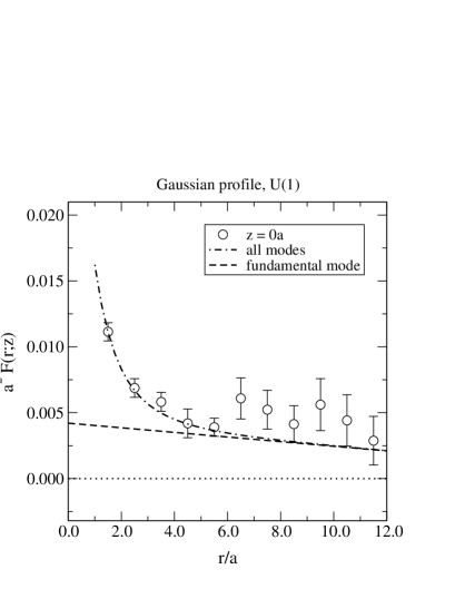
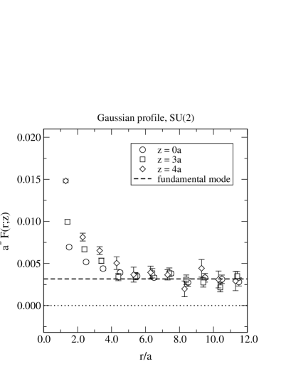
Figure 1: The force $F(r;z)$ for the Gaussian weight function, Eq. (5.1), at different fixed values of $z$, in the Abelian (left; volume = $48^{2}\times 14$) and non-Abelian cases (right; volume = $24^{2}\times 14$). The perturbative values are also shown. The Abelian case has a finite slope because of the periodicity discussed around Eq. (4.10).

We will start with a study of a Gaussian weight function,

$$\Delta(z)\equiv\Delta_{0}\exp\Bigl{(}-{\frac{1}{2}}m^{2}z^{2}\Bigr{)}\;.$$ (5.1)

The spectrum following from it is discussed in Appendix A.1, and goes as $m_{n}=\sqrt{n}m$, $n=0,1,2,...\;$. The zero mode, $\psi_{c}\equiv\psi_{0}$, does have a finite coupling in this case, since $\int_{z}\Delta(z)$ is finite. Note that even though the wave function $\psi_{c}$ is constant in $z$, this mode is said to have been localised, in the sense that $\Delta(z)\psi_{c}^{2}$ is centered around $z=0$.

The original theory has two parameters, $\Delta_{0},~{}m$. As both of them are dimensionful ($[\Delta_{0}]=$GeV^-1, $[m]=$GeV in (2+1)d), continuum physics only depends on their product. Moreover, the mass spectrum, and thus the dynamics of the Abelian theory, are completely independent of $\Delta_{0}$. Correspondingly, it appears that the non-Abelian theory can be made weakly interacting by choosing a large value of $m\cdot\Delta_{0}$. This argument might fail, however, because $m_{0}\cdot\Delta(z)$ is exponentially small at large $z$.

The lattice introduces a further dimensionful parameter, the lattice spacing $a$. It should be chosen small enough such that discretisation effects are harmless. Somewhat arbitrarily, we then fix $a,m,\Delta_{0}$ such that

$$(am)^{2}=0.1,\quad 4\Delta_{0}/a=60.0.$$ (5.2)

Thereby the theory should be weakly coupled ($m\cdot\Delta_{0}\approx 4.7$), and also close to continuum behaviour ($a\cdot m\approx 0.3$). The extent of the lattice in the $z$-direction is chosen as $14\,a\approx 4.4m^{-1}$ (cf. Fig. 1).

The massless zero mode present in the system should dominate the physics at large distances. Its coupling is independent of $z$ and, according to Eqs. (3.6), (3.8),

$$F(r;z)={\frac{1}{2}}C_{A}\psi_{c}^{2}=\frac{C_{A}}{2\int_{z^{\prime}}\Delta(z^{\prime})},$$ (5.3)

where $C_{A}=1$ for U(1), $3/4$ for SU(2). The other modes give exponentially suppressed contributions, according to Eq. (3.5).

In fact, we can easily make an exact continuum prediction for the full force $F(r;z)$ in the Abelian case. The analytic values of $m_{n}=\sqrt{n}m$ and $\psi_{n}(z=0)$ are given in Appendix A.1, and can be plugged into Eq. (4.10). The prediction is compared with numerical data in Fig. 1 (left). Although the data becomes noisy at large $r$, we can conclude that there is agreement within statistical errors, confirming that discretisation effects are under control.

The numerical result for $F(r;z)$ in the SU($2$) case is shown in Fig. 1 (right). It indicates that the large distance behaviour is successfully predicted by the perturbative analysis. Moreover, the fact that the constant value to which $F(r;z)$ tends does not depend on $z$ confirms that the constant mode dominates in that regime. We see also the divergence of $F(r;z)$ at small distances, as in the U($1$) data. Qualitatively, the U($1$) and SU($2$) cases yield very similar results. This is a peculiarity of 2d physics, however; had we compactified onto three dimensions, our expectation would be $F(r;z)\sim 1/r$ for U($1$), and yet still the confining constant force for SU($2$).

5.2 Sharp weight function

We next study a warped “sharp” weight function,

$$\Delta(z)\equiv\Delta_{0}\exp\Bigl{(}-M|z|+{\frac{1}{2}}m^{2}z^{2}\Bigr{)}\;.$$ (5.4)

The corresponding spectrum is discussed in Appendix A.2.

        

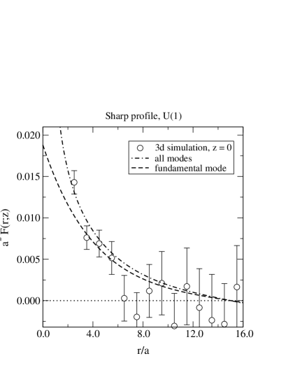
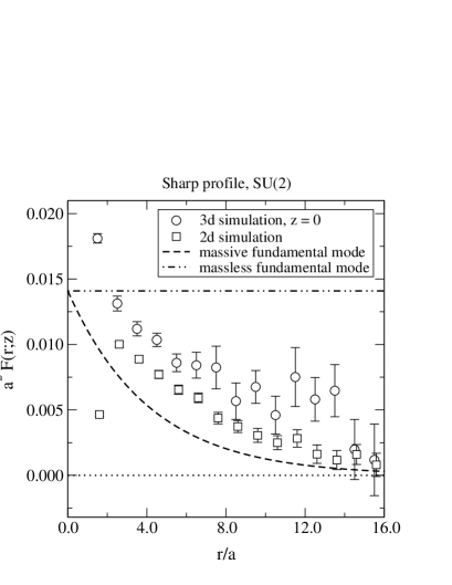
Figure 2: The force $F(r;z)$ for the sharp weight function, Eq. (5.4), at $z=0$ in the Abelian (left) and non-Abelian cases (right). In the Abelian case (where no noise reduction techniques were used) the force is anti-symmetric with respect to $r/a=15$. For comparison we also show the result from a 2d simulation based on Eq. (4.8).

In addition to the requirements for the Gaussian case above, leading to a weak effective coupling and small discretisation effects, we are now faced with an additional constraint, as well as an additional parameter allowing to satisfy it: we want to tune $M/m$ such that the “fundamental mode” $\psi_{0}(z)$, the one with the lightest non-zero mass $m_{0}$, is much lighter than the next mode, with mass $m_{1}$. This tends to make the choice of parameters somewhat less transparent. From the point of view of the infinite volume setup, the zero mode $\psi_{c}$ is an artifact of the simulation, whose effects ought also to be kept numerically small.

In practice, we choose the parameters as

$$am=0.50,\quad aM=0.75,\quad 4\Delta_{0}/a=35.0\;.$$ (5.5)

The spectrum resulting from these parameters is discussed in Appendix A.2. The mass of the “fundamental mode”, $m_{0}$, is $(m_{0}/m)^{2}=0.235$. In lattice units, therefore,

$${\xi_{0}}/{a}\equiv({am_{0}})^{-1}\approx 4.1\;.$$ (5.6)

The first excited state with a finite coupling $\psi_{n}(z)$ at $z=0$, on the other hand, has a correlation length $\xi_{2}/a\approx 1.4$. Thus the fundamental mode should indeed dominate the infrared physics. For the lattice size used, $30^{2}\times 18$, the effective couplings of the zero and fundamental mode are

$$a\psi_{c}\approx 0.048,\quad a\psi_{0}(0)\approx 0.194\;.$$ (5.7)

We observe that because of the finite volume, $a\psi_{c}$ is not quite zero yet. The contributions from the different modes to $a^{2}F(r;z)$ follow from Eq. (3.5) and, fortunately, the effect of $a\psi_{c}$ turns out to be smaller than our error bars. Note also that a dimensionless 2d effective coupling can be estimated as

$$\frac{\psi_{0}}{\pi m_{0}}\approx\frac{0.79}{\pi}\;,$$ (5.8)

and the parameters $\alpha_{3}$ and $\alpha_{4}$ defined in Eq. (3.10) evaluate to

$$\alpha_{3}=0.804\qquad\alpha_{4}=0.749,$$ (5.9)

suggesting that the perturbative picture, as well as a 2d action of the form in Eq. (4.8), should be qualitatively applicable.

The data is shown in Fig. 2. In the Abelian case, we insert the values of $\psi_{n}(z=0)$ and $m_{n}$ computed in Appendix A into Eq. (4.10), to obtain the continuum prediction, shown with the dashed-dotted line. The dashed line shows the contribution of the fundamental mode alone. The simulation is quite consistent with the exponential decay of $F(r;z)$. However, the periodicity in the $r$-direction makes the extraction of the force quite difficult and noisy when $r\approx L/2$.

In the SU($2$) case, the value of the fundamental mode prediction at $r=0$ sets the scale for the asymptotic confining force, were the fundamental mode massless (dashed-dotted line). Clearly, the lattice data is consistent rather with a decaying force, or the “breaking of the string”, on a distance scale given by $\xi_{0}=m_{0}^{-1}$. As a comparison, we show also the result for the 2d system, Eq. (4.8), using the tree-level values of $a\psi_{0}(0)$, $am_{0}$ as input. We observe the same qualitative behaviour, although the (2+1)-dimensional case leads to a stronger force at small distances, due to the exchange of higher modes.

Finally, we reiterate that because of the finite value of $a\psi_{c}$ in our finite box (cf. Eq. (5.7)), the 3d force should at very large distances still approach a finite non-vanishing value, $\sim 0.001$, which is however beyond our resolution.

5.3 Smooth weight function

We end by studying a “smooth” weight function,

$$\Delta(z)=\Delta_{0}\exp\Bigl{(}-{\frac{1}{2}}M^{2}z^{2}+{\frac{1}{4}}m^{4}z^{4}\Bigr{)}\;.$$ (5.10)

The corresponding spectrum is discussed in Appendix A.3.

        

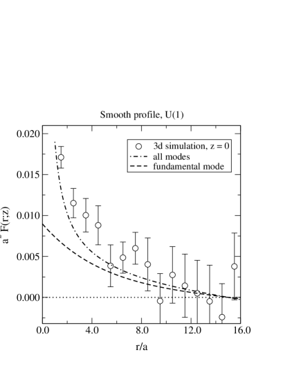
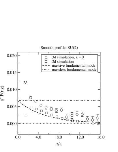
Figure 3: The force $F(r;z)$ for the smooth weight function, Eq. (5.10), at $z=0$, in the Abelian (left) and non-Abelian cases (right). In the Abelian case (where no noise reduction techniques were used) the force is anti-symmetric with respect to $r/a=15$. For comparison we also show the result from a 2d simulation based on Eq. (4.8).

We choose the parameters and lattice spacing such that

$$am=0.2778,\quad aM=0.3889,\quad 4\Delta_{0}/a=35.0\;.$$ (5.11)

According to Appendix A.3, the correlation length of the fundamental mode is then

$$\xi_{0}/a=(am_{0})^{-1}\approx 5.2.$$ (5.12)

The couplings of the zero and fundamental mode are, at $z=0$,

$$a\psi_{c}\approx 0.054,\quad a\psi_{0}(0)\approx 0.134.$$ (5.13)

These determine the string tension, according to Eq. (3.5). We also note that the dimensionless coupling related to the fundamental mode is

$$\frac{\psi_{0}}{\pi m_{0}}\approx\frac{0.69}{\pi}\;,$$ (5.14)

and the parameters $\alpha_{3}$ and $\alpha_{4}$ defined in Eq. (3.10) evaluate to

$$\alpha_{3}=0.705\qquad\alpha_{4}=0.695,$$ (5.15)

supporting again the qualitative applicability of the perturbative picture, as well as of the 2d action in Eq. (4.8).

The lattice simulation is carried out with the volume $30^{2}\times 18$. The data is shown in Fig. 3. We proceed as in the “sharp” case to compute the prediction for $F(r;z)$. The U($1$) data is consistent with the analytic prediction, although large statistical errors make this statement rather weak. For the SU($2$) case we again observe that the behaviour of the 3d simulation agrees at large distances within statistical errors with the massive fundamental mode prediction, as well as with results obtained with the 2d action in Eq. (4.8), using the tree-level values of $a\psi_{0}(0)$, $am_{0}$ as input. At smaller distances, the static force is stronger in the (2+1)-dimensional system, as noted previously. Note also again that because of the finite value of $a\psi_{c}$ in our finite box (cf. Eq. (5.13)), the 3d force should at very large distances still approach a finite non-vanishing value, $\sim 0.001$.

6 Conclusions

We have studied in this paper some physical properties of a pure gauge field theory, living in a space where the coupling constant $g^{2}(z)\equiv\frac{1}{\Delta(z)}$ varies along one spatial direction. Using a mode decomposition and working in the gauge $A_{z}=0$, an effective lower dimensional action was already derived in [1]. However, in the non-Abelian case, several complications arise: all Kaluza–Klein like modes are coupled through cubic and quartic terms, possible non-perturbative effects in regions where the coupling is large make the validity of the perturbative analysis unclear, and the naively truncated action for the low-energy sector is non-renormalisable. These difficulties motivated a lattice simulation of the non-Abelian theory in (2+1) dimensions, as well as, for calibration, simulations of the Abelian theory in the same background (in which case our analytic predictions are exact in the continuum limit).

In the case of a Gaussian profile $\Delta(z)$, our numerical data confirms the presence of a massless constant mode, which gives rise to a constant force both in the Abelian and the non-Abelian cases, in spite of the coupling becoming strong at large $z$. Note that even though the mode is constant in $z$, this mechanism is conventionally called the localisation of massless vector bosons, since $\Delta(z)\times$[the mode] is sharply centered.

For two different profiles such that $\int_{z}\Delta(z)=\infty$, on the other hand, where the massless mode decouples from the theory, the lattice data is consistent with the long distance dynamics being dominated by a single massive localised “fundamental” vector mode. Because of a large hierarchy between the mass $m_{0}$ of the fundamental mode, and those of the higher modes, this regime can set in even at distances somewhat smaller than the correlation length of the fundamental mode.

Thus we confirm the qualitative picture based on perturbation theory in these (2+1)-dimensional systems. It would be interesting to extend the study to a (3+1)-dimensional case, to check whether our conclusions depend on the peculiarities of the two-dimensional effective theory.

Appendix Appendix A Energy spectra for various weight functions

In this Appendix, we determine explicitly the spectra for the various weight functions appearing in this paper.

As mentioned in [1], we can write Eq. (2.6) in another form by introducing $\chi_{n}(z)=\sqrt{\Delta(z)}\psi_{n}(z)$. Then the eigenvalue equation takes the familiar form

$$-\chi_{n}^{\prime\prime}+V_{o}(z)\chi_{n}=m_{n}^{2}\chi_{n},$$ (A.1)

where

$$V_{o}(z)\equiv W^{2}(z)-W^{\prime}(z),\quad W(z)\equiv-\frac{\Delta^{\prime}(z)}{2\Delta(z)}.$$ (A.2)

One may also introduce

$$V_{s}(z)\equiv W^{2}(z)+W^{\prime}(z)\;;$$ (A.3)

its eigenvalues are the same as those of $V_{o}(z)$, except that one of the two has a normalisable exact zero mode, and the symmetry properties of the two sets of wave functions with the same energy are the opposite [29]. Thus, denoting $m_{n}^{2}=E^{(n)}$ and assuming $E_{s}^{(0)}=0$, we have $E_{o}^{(n)}=E_{s}^{(n+1)},n\geq 0$.

It is useful to note that if $\Delta(z)=\Delta_{0}\exp(f(z))$, then

$$W=-{\frac{1}{2}}f^{\prime},\quad V_{o}={\frac{1}{4}}(f^{\prime})^{2}+{\frac{1}{2}}f^{\prime\prime}\;.$$ (A.4)

Therefore, the eigenvalues are independent of $\Delta_{0}$.

A.1 Gaussian weight function

We start by considering the Gaussian weight function, Eq. (5.1), which implies that

$$W=\frac{1}{2}m^{2}z,\quad V_{o}={\frac{1}{2}}m^{2}\Bigl{(}{\frac{1}{2}}m^{2}z^{2}-1\Bigr{)}\;.$$ (A.5)

The eigenvalue equation, Eq. (A.1), is just of the form of a harmonic oscillator, with shifted energy levels, and is immediately solved. We obtain

$$m_{n}=m\sqrt{n},\quad n\geq 0.$$ (A.6)

Note the existence of a normalisable zero energy solution. It appears here for $V_{o}$ rather than $V_{s}$, since $\int_{z}\Delta(z)$ is finite.

We also know the wave functions exactly in this case,

$$\psi_{n}(z)=\frac{1}{2^{n/2}}~{}\frac{1}{\pi^{1/4}\sqrt{\Delta_{0}}}~{}\frac{1}{\sqrt{n!}}~{}H_{n}\Bigl{(}\frac{mz}{\sqrt{2}}\Bigr{)},$$ (A.7)

where $H_{n}$ are the Hermite polynomials. Using the fact that $H_{n}$ have the parity of their index and that

$$H_{2n}(z=0)=(-1)^{n}~{}\frac{(2n)!}{n!},$$ (A.8)

we arrive at the expression

$$\psi_{2n}(z=0)=\frac{1}{\pi^{1/4}\sqrt{\Delta_{0}}}\left(-\frac{1}{2}\right)^{n}\frac{\sqrt{(2n)!}}{n!}\sim\frac{(-1)^{n}}{\sqrt{\pi\Delta_{0}}}~{}\frac{1}{n^{1/4}}\;,$$ (A.9)

where the last step is the large $n$ asymptotic behaviour. This means that the higher modes are not only more massive, but also more weakly coupled at $z=0$.

A.2 “Sharp” weight function

        

Figure 4: Left: The fundamental mode $\psi_{0}(z)$ and the profile $\Delta(z)$ for the sharp wave function, Eq. (5.4), at $c=M/m=1.5$, $R=4.5/m$, and a specific $a$ (see Table 1). The horizontal axis is for $\zeta=zm$. Right: the first excited even modes.

The sharp weight function, Eq. (5.4), leads to

$$W={\frac{1}{2}}(M\mathop{\mbox{sign}}(z)-m^{2}z)\;.$$ (A.10)

It is convenient to rescale everything by $m$: $\zeta\equiv mz$, $c\equiv M/m$, $\nu_{n}\equiv m_{n}^{2}/m^{2}$. Eq. (A.1) then becomes

$$-\chi_{n}^{\prime\prime}+\Bigl{[}{\frac{1}{4}}(\zeta-c\mathop{\mbox{sign}}(\zeta))^{2}+{\frac{1}{2}}-c\,\delta(\zeta)\Bigr{]}\chi_{n}=\nu_{o}^{(n)}\chi_{n}.$$ (A.11)

The solutions only depend on $c$. Note that although we are using the same notation as in Eq. (A.1), $\chi_{n}$ is here treated as a function of $\zeta$ rather than $z$.

Since the Hamiltonian is invariant under parity, one can classify its eigenfunctions as symmetric and antisymmetric under $\zeta\to-\zeta$. We label symmetric and antisymmetric states with even and odd indices, respectively.

Infinite volume. We start by discussing the infinite volume case. Here we solve the problem by utilising $V_{s}$. Note that, apart from the usual relation $E_{o}^{(n)}=E_{s}^{(n+1)}$, $n\geq 0$, there is now the additional relation that the eigenvalues obtained with $V_{s}$ and $V_{o}$, coming with wave functions antisymmetric in ($z\to-z$), are trivially related by the addition of $m^{2}$, because the antisymmetric state does not “see” the $\delta$ function at the origin. This can be expressed as $E_{o}^{(p)}=E_{s}^{(p)}+m^{2}$, for $p$ odd. Therefore, the spectrum is of the form

$$E_{o}^{(0)} = E_{s}^{(1)}=\epsilon,$$ (A.12)

$$E_{o}^{(1)} = E_{s}^{(1)}+m^{2}=E_{s}^{(2)},$$ (A.13)

$$E_{o}^{(2)} = E_{s}^{(3)}>E_{s}^{(2)},...\;.$$ (A.14)

In other words, $V_{s}$ has a symmetric state with exactly zero energy, and an antisymmetric one with an exponentially small energy, $\epsilon$ (cf. Eq. (A.26) below). Then $V_{o}$ has a symmetric ground state with the energy $\epsilon$, and a doublet of states with a much higher energy, $E_{s}^{(3)}\approx E_{s}^{(2)}\gg\epsilon$.

The explicit form of the dimensionless equation with $V_{s}$ becomes

$$-\chi_{n}^{\prime\prime}+\Bigl{[}{\frac{1}{4}}(\zeta-c\mathop{\mbox{sign}}(\zeta))^{2}-{\frac{1}{2}}+c\delta(\zeta)\Bigr{]}\chi_{n}=\nu^{(n)}_{s}\chi_{n}.$$ (A.15)

Introducing the Kummer function

$$\phi(a;b;\zeta)=1+\frac{a}{b}\frac{\zeta}{1!}+\frac{a(a+1)}{b(b+1)}\frac{\zeta^{2}}{2!}+\dots=\sum_{n=0}^{\infty}\frac{(a)_{n}}{(b)_{n}}\frac{\zeta^{n}}{n!},$$ (A.16)

which satisfies

$$\zeta\frac{d^{2}\phi}{d\zeta^{2}}+(b-\zeta)\frac{d\phi}{d\zeta}-a\phi=0\;,$$ (A.17)

the general solution of Eq. (A.15) reads, for $\zeta\neq 0$ and denoting $\nu^{(n)}_{s}\to\nu$,

$$\chi(\zeta)=e^{-\frac{(|\zeta|-c)^{2}}{4}}\left[A\,\phi(-\frac{\nu}{2};\frac{1}{2};\frac{(|\zeta|-c)^{2}}{2})+B\,(|\zeta|-c)\,\phi(\frac{1-\nu}{2};\frac{3}{2};\frac{(|\zeta|-c)^{2}}{2})\right],$$ (A.18)

where $A,B$ are constants. For $\zeta<0$, we denote $\chi$ by $\chi_{L}$, with constants $A_{L},B_{L}$, and for $\zeta>0$, $\chi_{R}$, with $A_{R},B_{R}$. The symmetric wave functions obviously have $A_{L}=A_{R},B_{L}=B_{R}$, the antisymmetric ones $A_{L}=-A_{R},B_{L}=-B_{R}$.

The boundary conditions we have to impose on the coefficients are:

• $\chi_{R}(0)=\chi_{L}(0)$,

• $\chi_{R}^{\prime}(0)=\chi_{L}^{\prime}(0)+c\,\chi_{L,R}(0)$,

• $\lim_{\zeta\to\infty}\chi_{R}(\zeta)=\lim_{\zeta\to-\infty}\chi_{L}(\zeta)=0\;.$

The second comes from integrating both sides of Eq. (A.15) from $-\delta$ to $\delta$.

In both the symmetric and antisymmetric cases, the third condition imposes

$$B_{R}=-\sqrt{2}\frac{\Gamma(\frac{1-\nu}{2})}{\Gamma(-\frac{\nu}{2})}A_{R},$$ (A.19)

where we used that for large $\zeta$,

$$\phi(a;b;\zeta)\approx e^{\zeta}\zeta^{a-b}\frac{\Gamma(b)}{\Gamma(a)}.$$ (A.20)

For symmetric wave functions, the condition (a) is automatically satisfied. The condition (b) yields

$$B_{R}=\frac{c\phi_{1}^{\prime}}{\phi_{3}+c^{2}\phi_{3}^{\prime}}A_{R}\;,$$ (A.21)

where $\phi_{1}^{\prime}\equiv\phi^{\prime}(-\frac{\nu}{2};\frac{1}{2};\frac{c^{2}}{2})$, $\phi_{3}\equiv\phi(\frac{1-\nu}{2};\frac{3}{2};\frac{c^{2}}{2})$, $\phi_{3}^{\prime}\equiv\phi^{\prime}(\frac{1-\nu}{2};\frac{3}{2};\frac{c^{2}}{2})$. Combining this with Eq. (A.19), one obtains an algebraic equation for the energy levels:

$$-\nu\,c\,\phi(1-\frac{\nu}{2};\frac{3}{2};\frac{c^{2}}{2})+\sqrt{2}\frac{\Gamma(\frac{1-\nu}{2})}{\Gamma(-\frac{\nu}{2})}\Bigl{[}\phi(\frac{1-\nu}{2};\frac{3}{2};\frac{c^{2}}{2})+c^{2}\frac{1-\nu}{3}\phi(\frac{3-\nu}{2};\frac{5}{2};\frac{c^{2}}{2})\Bigr{]}=0,$$ (A.22)

where we made use of

$$\phi^{\prime}(a;b;\zeta)=\frac{a}{b}\phi(a+1;b+1;\zeta)\;.$$ (A.23)

Note that since $\Gamma(-\nu/2)$ has a pole at $\nu=0$, $\nu=0$ is a solution for any $c$, as must be the case.

For antisymmetric wave functions, the condition (a) yields

$$B_{R}=\frac{\phi_{1}}{c\phi_{3}}A_{R}\;,$$ (A.24)

with the same notation as above. The condition (b) is then automatically satisfied. Together with Eq. (A.19), one again obtains an algebraic equation for the energy levels:

$$\Gamma(-\frac{\nu}{2})\phi(-\frac{\nu}{2};\frac{1}{2};\frac{c^{2}}{2})+\sqrt{2}\,c\,\Gamma(\frac{1-\nu}{2})\phi(\frac{1-\nu}{2};\frac{3}{2};\frac{c^{2}}{2})=0\;.$$ (A.25)

In the limit $c\gg 1$, the approximate solution for the lowest energy level is obtained by setting $\nu\to 0$ in the argument of the first $\phi$ appearing, whereby $\phi(0;{\frac{1}{2}};{\frac{c^{2}}{2}})=1$; we then get

$$\nu_{o}^{(0)}=\nu_{s}^{(1)}\approx\sqrt{{2}/{\pi}}\,c\,e^{-\frac{c^{2}}{2}}.$$ (A.26)

Some numerical values for $\nu$ (expressed as $\nu^{(n)}_{o}=\nu^{(n+1)}_{s}$) are included in Table 1.

Finite volume. Let us now consider the same system, but in a box with periodic boundary conditions at $\zeta=\pm R/m\equiv\pm\hat{R}$, rather than in infinite volume:

$$\chi_{L}(-\hat{R})=\chi_{R}(\hat{R}).$$ (A.27)

Then the spectrum changes. We will study this system directly in terms of $V_{o}$, rather than $V_{s}$. The general form of the solution in terms of the Kummer functions remains the same, except that the Hamiltonian at $\zeta\neq 0$ has changed by a constant.

We will now need to impose a boundary condition at $\zeta=\hat{R}$. Integrating the equation of motion for $\psi$ from $\hat{R}-\delta$ to $\hat{R}+\delta$, it is easily seen that $\psi^{\prime}$ must be continuous at $\zeta=\hat{R}$ (because $\Delta$ is). This translates into

$$\chi_{R}^{\prime}(\hat{R})+\hat{W}(\hat{R})\chi_{R}(\hat{R})=0\;,$$ (A.28)

where $\hat{W}\equiv W/m$. This means that $\chi$’s derivative is not continuous at the boundary, which is due to the discontinuity of $\Delta^{\prime}$ at $\zeta=\hat{R}$. The other boundary condition for the symmetric states is Eq. (A.28) applied at the origin or, equivalently, condition (b) above,

$$\chi_{R}^{\prime}(0)+\hat{W}(0)\chi_{R}(0)=0\;.$$ (A.29)

Note that Eqs. (A.28), (A.29) imply that $\psi_{R}^{\prime}(0)=\psi_{R}^{\prime}(R)=0$. In the antisymmetric case, the complete boundary conditions are

$$\chi_{R}(0)=0,\qquad\chi_{R}(\hat{R})=0,$$ (A.30)

and Eq. (A.28) then imposes that $\chi^{\prime}_{R}(\hat{R})$ vanish as well.

For symmetric wave functions, Eq. (A.29) implies

$$A_{R}=DB_{R},\qquad D\equiv\frac{(1-c^{2})\phi_{3}+c^{2}\phi_{3}^{\prime}}{c(\phi_{1}^{\prime}-\phi_{1})},$$ (A.31)

where the notation is as above. Inserting into Eq. (A.28),

$$\Bigl{[}1-(\hat{R}-c)^{2}\Bigr{]}\phi_{3}^{\hat{R}}+(\hat{R}-c)^{2}\phi_{3}^{\prime\hat{R}}+(\hat{R}-c)(\phi_{1}^{\prime\hat{R}}-\phi_{1}^{\hat{R}})D=0,$$ (A.32)

where $\phi_{1}^{\hat{R}}\equiv\phi(-\frac{\nu}{2};\frac{1}{2};\frac{(\hat{R}-c)^{2}}{2})$, $\phi_{1}^{\prime\hat{R}}\equiv\phi^{\prime}(-\frac{\nu}{2};\frac{1}{2};\frac{(\hat{R}-c)^{2}}{2})$, $\phi_{3}^{\hat{R}}\equiv\phi(\frac{1-\nu}{2};\frac{3}{2};\frac{(\hat{R}-c)^{2}}{2})$, $\phi_{3}^{\prime\hat{R}}\equiv\phi^{\prime}(\frac{1-\nu}{2};\frac{3}{2};\frac{(\hat{R}-c)^{2}}{2})$. This equation determines $\nu$, after which the actual energy level is found by adding 1.

For antisymmetric wave functions, Eqs. (A.30) imply that

$$B_{R}=\frac{\phi_{1}}{c\phi_{3}}A_{R},\qquad B_{R}=\frac{\phi_{1}^{\hat{R}}}{(c-\hat{R})\phi_{3}^{\hat{R}}}A_{R}\;.$$ (A.33)

These are compatible only if

$$(c-\hat{R})\phi_{1}\phi_{3}^{\hat{R}}=c\phi_{3}\phi_{1}^{\hat{R}}\;,$$ (A.34)

which determines the eigenvalues.

	sharp profile, $c=1.5$			sharp profile, $c=2.5$
	$\hat{R}=4.5$		$\hat{R}=\infty$	$\hat{R}=4.5$		$\hat{R}=\infty$
$n$	$\nu_{o}^{(n)}$	$a\psi_{n}(0)$	$\nu_{o}^{(n)}$	$\nu_{o}^{(n)}$	$a\psi_{n}(0)$	$\nu_{o}^{(n)}$
$c$	0.000	0.048	—	0.000	0.201	—
$0$	0.235	0.194	0.209	0.154	0.148	0.038
$1$	1.235	0.000	1.209	1.154	0.000	1.038
$2$	1.945	0.116	1.643	1.815	0.101	1.191
$3$	2.945	0.000	2.643	2.815	0.000	2.191
$4$	4.432	0.113	3.201	4.298	0.106	2.478
$5$	5.432	0.000	4.201	5.298	0.000	3.478
$6$	7.854	0.112	4.829	7.723	0.109	3.867
$7$	8.854	0.000	5.829	8.723	0.000	4.867
$8$	12.24	0.112	6.504	12.11	0.110	5.327
$9$	13.24	0.000	7.504	13.11	0.000	6.327

Table 1: Eigenvalues for the sharp profile. For the wave functions at origin one needs also the values of $am,\Delta_{0}/a$, entering as $a\psi_{n}(0)\propto(am)^{1/2}(\Delta_{0}/a)^{-1/2}$, if $c,\hat{R}$ are kept fixed; we have assumed $am=0.5,\Delta_{0}/a=8.75$, for both values of $c$.

As an example, some numerical values are given in Table 1. The doublet structure as discussed above is visible in the infinite volume results (levels 1 & 2; 3 & 4; …). It can also be observed that for small $n$, the spectrum is roughly linear in $n$ (like in Eq. (A.6) for $m_{n}^{2}$), while for large values within a finite box, it starts to resemble more the corresponding spectrum $\sim n^{2}$.

A.3 “Smooth” weight function

        

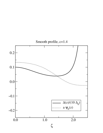
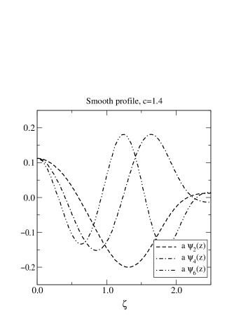
Figure 5: Left: The fundamental mode $\psi_{0}(z)$ and the profile $\Delta(z)$ for the smooth wave function, Eq. (5.10), at $c=M/m=1.4$, $R=2.5/m$, and a specific $a$ (see Table 2). The horizontal axis is for $\zeta=zm$. Right: the first excited even modes.

The smooth weight function, Eq. (5.10), leads to

$$W={\frac{1}{2}}(M^{2}z-m^{4}z^{3})\;.$$ (A.35)

We rescale again everything by $m$: $\zeta=mz$, $c=M/m$, $\nu_{n}=m_{n}^{2}/m^{2}$. Eq. (A.1) then becomes

$$-\chi_{n}^{\prime\prime}+\Bigl{[}{\frac{1}{4}}\zeta^{2}(c^{2}-\zeta^{2})^{2}-{\frac{1}{2}}c^{2}+{\frac{3}{2}}\zeta^{2}\Bigr{]}\chi_{n}=\nu_{o}^{(n)}\chi_{n}.$$ (A.36)

The solutions thus only depend on $c$. The boundary conditions are as in Eqs. (A.28), (A.29), (A.30), for the symmetric and antisymmetric cases, respectively.

	smooth profile, $c=1.4$			smooth profile, $c=2.0$
	$\hat{R}=2.5$		$\hat{R}=\infty$	$\hat{R}=3.15$		$\hat{R}=\infty$
$n$	$\nu_{o}^{(n)}$	$a\psi_{n}(0)$	$\nu_{o}^{(n)}$	$\nu_{o}^{(n)}$	$a\psi_{n}(0)$	$\nu_{o}^{(n)}$
$c$	0.000	0.054	—	0.000	0.034	—
$0$	0.484	0.134	0.388	0.033	0.112	0.030
$1$	3.020	0.000	3.016	3.310	0.000	3.310
$2$	6.154	0.112	5.862	5.517	0.065	5.513
$3$	9.430	0.000	9.373	7.912	0.000	7.912
$4$	14.48	0.112	13.50	11.16	0.075	11.15
$5$	18.51	0.000	18.17	14.95	0.000	14.95
$6$	25.83	0.112	23.32	19.27	0.075	19.21
$7$	30.17	0.000	28.92	23.92	0.000	23.92
$8$	40.20	0.112	34.95	29.20	0.074	29.03
$9$	44.63	0.000	41.37	34.57	0.000	34.54

Table 2: Eigenvalues for the smooth profile. For the wave functions at origin one needs also the values of $am,\Delta_{0}/a$, entering as $a\psi_{n}(0)\propto(am)^{1/2}(\Delta_{0}/a)^{-1/2}$, if $c,\hat{R}$ are kept fixed; we have assumed $am=5.0/18.0,\Delta_{0}/a=8.75$, for $c=1.4$; and $am=0.45,\Delta_{0}/a=25.0$, for $c=2.0$.

This time we have only solved the eigenvalue problem numerically. The profile $\Delta(z)$, the fundamental wave function $\psi_{0}(z)$, as well as the first excited symmetric wave functions, are shown in Fig. 5, for $c=M/m=1.4$. Examples of eigenvalues are given in Table 2.

Appendix Appendix B Gauge invariant correlators in the Abelian case

In the Abelian theory, Eq. (2.1), the field strength tensor $F_{\mu\nu}$ is gauge invariant. This allows one to measure directly various gauge invariant correlation functions displaying the essential features of the spectrum $\{m_{n}\}$, as we will show with a specific example. These correlators are however not available in the non-Abelian case. Other possibilities exist, but they contain either composite operators, making a qualitative distinction between genuinely confining and Higgs-like phases difficult, or non-local operators, making the analysis of ultraviolet divergences as well as practical measurements hard.

Let us define

$${\cal O}_{p}(x;z) = \frac{1}{T}\int\!{\rm d}t\,F_{xt}(x,t,z)e^{ipt},$$ (B.1)

$${\cal O}^{(n)}_{p}(x) = \int_{z}\Delta(z)\psi_{n}(z){\cal O}_{p}(x;z)\;.$$ (B.2)

We might then consider, e.g., a weighted average over the $z$-direction,

$$G^{({\mbox{\scriptsize all}})}_{p}(r)\equiv\int_{z}\Delta(z)\int\!{\rm d}x\,{\cal O}_{p}(x;z)[{\cal O}_{p}(x+r;z)]^{*},$$ (B.3)

or, alternatively, a correlator only getting a contribution from some specified mode,

$$G^{(n)}_{p}(r) \equiv \int\!{\rm d}x\,{\cal O}^{(n)}_{p}(x)[{\cal O}^{(n)}_{p}(x+r)]^{*}.$$ (B.4)

Employing the unitary gauge propagator (${\bf p},{\bf x},{\bf x}^{\prime}$ are 2d vectors)

$$\langle F^{m}_{xt}({\bf x})F^{n}_{xt}({\bf x}^{\prime})\rangle=\int\frac{{\rm d}^{2}p}{(2\pi)^{2}}\frac{p^{2}}{p^{2}+m_{n}^{2}}\delta^{mn}e^{i{\bf p}\cdot({\bf x}-{\bf x}^{\prime})},$$ (B.5)

one easily finds

$$G^{({\mbox{\scriptsize all}})}_{p}(r) = \sum_{n}G^{(n)}_{p}(r),$$ (B.6)

$$G^{(n)}_{p}(r) = \delta(r)-\frac{m_{n}^{2}}{2\sqrt{p^{2}+m_{n}^{2}}}e^{-|r|\sqrt{p^{2}+m_{n}^{2}}}\;.$$ (B.7)

Therefore, the spectrum $\{m_{n}\}$ again manifests itself in the form of the exponential decay. Note that in contrast to the force $F(r;z)$, however, the wave functions $\psi_{n}(z)$ do not appear in these predictions.

Appendix Appendix C The SU($N_{c}$) string tension in 2d

In this section we recall briefly the results for the static potential of pure SU($N_{c}$) gauge theory in two dimensions. For a more detailed discussion see, e.g., ref. [30].

The result for the Abelian case is shown in Eq. (3.3), with $\sum_{n}\psi_{n}^{2}(z)\to 1$. In the non-Abelian case, that result is at leading order simply multiplied by an additional factor $C_{A}=(N_{c}^{2}-1)/(2N_{c})$, coming from the sum over the Hermitian generators of the fundamental representation, $\sum_{a}T^{a}T^{a}$. If we define $C_{A}=1$ for U(1), the leading order result is then as written in Eqs. (3.5), (3.8).

It remains to show that there are no higher order corrections in the non-Abelian case. The naive argument goes as follows. As the potential is gauge fixing independent by construction, we can choose the gauge $A_{t}=0$. But then the cubic and quartic interactions vanish, so that indeed no further corrections should arise.

References

- [1] M.E. Shaposhnikov and P. Tinyakov, Phys. Lett. B 515 (2001) 442 [hep-th/0102161].
- [2] W.A. Bardeen and K. Shizuya, Phys. Rev. D 18 (1978) 1969.
- [3] B.W. Lee, C. Quigg and H.B. Thacker, Phys. Rev. D 16 (1977) 1519.
- [4] T. Appelquist and C. Bernard, Phys. Rev. D 22 (1980) 200.
- [5] L. Randall and R. Sundrum, Phys. Rev. Lett. 83 (1999) 4690 [hep-th/9906064].
- [6] G.R. Dvali and M.A. Shifman, Phys. Lett. B 396 (1997) 64; ibid. B 407 (1997) 452 (E) [hep-th/9612128].
- [7] N. Tetradis, Phys. Lett. B 479 (2000) 265 [hep-ph/9908209].
- [8] B. Bajc and G. Gabadadze, Phys. Lett. B 474 (2000) 282 [hep-th/9912232].
- [9] I. Oda, Phys. Lett. B 496 (2000) 113 [hep-th/0006203].
- [10] S.L. Dubovsky, V.A. Rubakov and P.G. Tinyakov, JHEP 0008 (2000) 041 [hep-ph/0007179].
- [11] G.R. Dvali, G. Gabadadze and M.A. Shifman, Phys. Lett. B 497 (2001) 271 [hep-th/0010071].
- [12] A. Kehagias and K. Tamvakis, Phys. Lett. B 504 (2001) 38 [hep-th/0010112].
- [13] A. Neronov, Phys. Rev. D 64 (2001) 044018 [hep-th/0102210].
- [14] V.A. Rubakov, Phys. Usp. 44 (2001) 871 [Usp. Fiz. Nauk 171 (2001) 913] [hep-ph/0104152].
- [15] M. Giovannini, Phys. Rev. D 66 (2002) 044016 [hep-th/0205139].
- [16] S. Randjbar-Daemi and M. Shaposhnikov, Nucl. Phys. B 645 (2002) 188 [hep-th/0206016].
- [17] P. Dimopoulos, K. Farakos, A. Kehagias and G. Koutsoumbas, Nucl. Phys. B 617 (2001) 237 [hep-th/0007079].
- [18] D.J. Gross, R.D. Pisarski and L.G. Yaffe, Rev. Mod. Phys. 53 (1981) 43.
- [19] N. Weiss, Phys. Rev. D 24 (1981) 475; Phys. Rev. D 25 (1982) 2667.
- [20] Y. Hosotani, Phys. Lett. B 126 (1983) 309.
- [21] C.P. Korthals Altes and M. Laine, Phys. Lett. B 511 (2001) 269 [hep-ph/0104031]; K. Farakos et al., hep-ph/0207343.
- [22] J. Zinn-Justin, “Quantum Field Theory and Critical Phenomena”, Chapter 18 (Oxford University Press, 1993).
- [23] M. Lüscher and P. Weisz, JHEP 0109 (2001) 010 [hep-lat/0108014]; JHEP 0207 (2002) 049 [hep-lat/0207003].
- [24] N. Cabibbo and E. Marinari, Phys. Lett. B 119 (1982) 387.
- [25] A.D. Kennedy and B.J. Pendleton, Phys. Lett. B 156 (1985) 393.
- [26] S.L. Adler, Phys. Rev. D 23 (1981) 2901.
- [27] P. de Forcrand and C. Roiesnel, Phys. Lett. B 151 (1985) 77.
- [28] M. Albanese et al. [APE Collaboration], Phys. Lett. B 192 (1987) 163.
- [29] F. Cooper, A. Khare and U. Sukhatme, Phys. Rept. 251 (1995) 267 [hep-th/9405029].
- [30] N.E. Bralić, Phys. Rev. D 22 (1980) 3090.