SLAC-PUB-9571 NLO Higgs boson rapidity distributions at hadron colliders

Abstract

We describe a new method, based on an extension of the unitarity cutting rules proposed in Ref. [2], which is very efficient for the algorithmic evaluation of phase-space integrals for various differential distributions. As a first application, we compute the next-to-leading order normalized rapidity distribution of the CP-even and the CP-odd Higgs boson produced in hadron collisions through gluon fusion. We work in the heavy top-quark approximation; we find that the NLO corrections at the LHC are approximately $5\%$ in the zero rapidity region.

1 Introduction

One of the major tasks of the Tevatron and the LHC is to discover and explore the so far inaccessible Higgs boson sector of the Standard Model (SM). The discovery of a single CP conserving Higgs boson, as predicted by its minimal version, or a more prolific spectrum of Higgs bosons, characteristic to extensions of the SM such as the minimal supersymmetric SM (MSSM) or the two-Higgs-doublet-model (2HDM) will elucidate the nature of electroweak symmetry breaking.

The dominant mechanism for the production of light Higgs bosons at hadron colliders is gluon fusion through a heavy quark loop. The production cross sections of both the CP-even ($H$) and the CP-odd ($A$) Higgs bosons are known exactly through next-to-leading order (NLO) in perturbative QCD [1] and through next-to-next-to-leading order (NNLO) only in the infinite top-quark mass approximation [2, 3]. Note that, in the case of the CP-odd Higgs boson, this approximation is reliable for small values of $\tan\beta\leq 10$, where the contributions of bottom-quark loops can be ignored. The double differential rapidity and $p_{T}$ distribution for the SM Higgs boson has been calculated through NLO by means of a fully differential Monte-Carlo program[4], and analytically [5] in the case of non-zero $p_{T}$. For the CP-odd Higgs the double differential rapidity and $p_{T}$ distribution was also calculated recently [6].

In this paper, we compute the NLO rapidity distributions for the production of the CP-even and CP-odd Higgs bosons analytically, including the virtual corrections at zero rapidity. This is formally one order lower in $\alpha_{s}$ than the NLO contributions of Refs. [4, 5, 6]. (Some numerical results for this distribution, including detector cuts, have been reported previously [7].) For the computation of the inclusive phase-space integrals for fixed Higgs boson rapidity we extend the method of Ref. [2] to accommodate the calculation of differential distributions. The idea is to replace the $\delta$-function constraint on the phase-space by an “effective” propagator. This propagator depends on the constraint and in general differs from conventional particle propagators; however, if the constraint is polynomial in external momenta, the resulting Feynman integrals can efficiently be dealt with by algebraic means. We will illustrate how this method works in the next Section. As a cross-check, we have also computed the rapidity distributions by explicitly integrating the finite remainders of the phase-space integrals after dipole subtraction [8]. We found complete agreement between the two methods.

2 Method

For the calculation we use the large top-quark mass $(m_{t}\to\infty)$ approximation which is known to work extremely well [1], even for relatively large Higgs boson masses. In this limit the interaction of the Higgs boson with gluons is given by an effective Lagrangian [1, 9] which is known to NNLO in the strong coupling constant. Keeping only the terms relevant to an NLO calculation, the CP-even and CP-odd effective Lagrangians read:

$${\cal L}_{eff}^{H}=-\frac{1}{4v}C_{1}^{H}\,H\,G_{\mu\nu}^{a}G^{a\mu\nu}\,,$$ (1)

$${\cal L}_{eff}^{A}=\frac{1}{v\tan\beta}C_{1}^{A}\,A\,G_{\mu\nu}^{a}\tilde{G}^{a\mu\nu}\,,$$ (2)

where $G_{\mu\nu}^{a}$ is the gluon strength tensor, $\tilde{G}_{\mu\nu}=\epsilon_{\mu\nu\alpha\beta}G^{\alpha\beta}$, $H,A$ are the Higgs boson fields, and $v\simeq 246$ GeV is the Higgs boson vacuum expectation value. The Wilson coefficients $C_{1}^{H,A}$, defined in the $\overline{{\rm MS}}$ scheme, are [9]:

$$C_{1}^{H}=-\frac{\alpha_{s}}{3\pi}\Bigg{\{}1+\frac{11}{4}\frac{\alpha_{s}}{\pi}\Bigg{\}}\,,$$ (3)

$$C_{1}^{A}=-\frac{\alpha_{s}}{16\pi}\,,$$ (4)

where $\alpha_{s}=\alpha_{s}(\mu)$ is the $\overline{{\rm MS}}$ strong coupling constant defined in the theory with $n_{f}=5$ active flavors.

We consider the collision of two hadrons with momenta $P_{1}=\sqrt{s}/{2}\left(1,{\bf 0}_{\perp},1)\right)$ and $P_{2}=\sqrt{s}/{2}\left(1,{\bf 0}_{\perp},-1\right)$, producing a Higgs boson $h=\{H,A\}$ with momentum $P_{h}=(E,{\bf p_{T}},p_{z})$. The rapidity $Y$ is defined by:

$$Y=\frac{1}{2}\log\left(\frac{E+p_{z}}{E-p_{z}}\right).$$ (5)

The hadronic rapidity distribution is obtained from the partonic rapidity distributions by convoluting them with appropriate parton densities:

$$\frac{d\sigma^{h}}{dY}=\sum_{i,j}\int_{0}^{1}dx_{1}dx_{2}f_{i}(x_{1})f_{j}(x_{2})\frac{d\sigma^{h}_{ij}}{dY}.$$ (6)

The partonic rapidity distributions for the hard scattering of partons $i,j$ with momenta $p_{1}=x_{1}P_{1}$ and $p_{2}=x_{2}P_{2}$ respectively, are obtained by integrating the hard scattering matrix elements over the phase-space of the final-state particles with the rapidity of the Higgs boson kept fixed:

$$\frac{d\sigma^{h}_{ij}}{2e^{2Y}dY}=\int d\Pi_{f}\left|{\cal M}^{h}_{ij}\right|^{2}\delta\left(e^{2Y}-\frac{E+p_{z}}{E-p_{z}}\right)\,.$$ (7)

In the center of mass frame of the colliding hadrons, the rapidity constraint can be written as:

$$\delta\left(e^{2Y}-\frac{E+p_{z}}{E+p_{z}}\right)=e^{-2Y}\delta\left(\frac{P_{h}\cdot\left[p_{1}-up_{2}\right]}{P_{h}\cdot p_{1}}\right)$$ (8)

with $u=\left(x_{1}/x_{2}\right)e^{-2Y}$.

At leading order in $\alpha_{s}$ a sole Higgs boson is produced; in this case momentum conservation renders the phase-space integrals trivial. At NLO, the production of the Higgs boson is accompanied by a production of either a quark or a gluon. This makes the phase-space integrations more complicated, but they are still sufficiently simple to be done directly. (See for example Ref. [10] for the analogous case of Drell-Yan production.) However, the brute force approach becomes cumbersome at NNLO and beyond.

In this paper we show how to compute the NLO contributions using a method suitable for an algorithmic evaluation of the rapidity distribution at NNLO as well. The idea is to replace the $\delta$-function constraint on the phase space in Eq. (8) in terms of the imaginary part of an effective “propagator”:

$$\delta(x)\to\frac{1}{2\pi i}\left[\frac{1}{x-i0}-\frac{1}{x+i0}\right].$$ (9)

We can then map the constrained phase space integrals onto loop integrals in a manner similar to what was suggested for unconstrained phase-space integrals in Ref. [2]. It is important that the constraint in Eq. (8) is a polynomial in momenta; this property allows the application of multi-loop algebraic techniques, such as integration-by-parts and recurrence relations [11], to the integrals produced after the mapping (9).

At NLO, using Eqs. (8,9), we can express all the phase-space integrals through linear combinations of the following loop integrals:

$$I(\nu_{1},\ldots,\nu_{5})=\int\frac{d^{d}k}{(2\pi)^{d}}\frac{1}{A_{1}^{\nu_{1}}\cdots A_{5}^{\nu_{5}}},$$ (10)

where

$$A_{1} = k^{2}-m_{h}^{2}\pm i\delta,$$ (11)

$$A_{2} = (k+p_{1})^{2},$$ (12)

$$A_{3} = (k+p_{1}+p_{2})^{2}\pm i\delta,$$ (13)

$$A_{4} = (k+p_{2})^{2},$$ (14)

$$A_{5} = k\cdot p_{1}-uk\cdot p_{2}\pm i\delta.$$ (15)

The propagators $A_{1}$, $A_{3}$ and $A_{5}$ are “cut” according to Eq. (9).

We now proceed to the reduction of the integrals of the above topology. It turns out that we can derive a sufficient set of recurrence relations through partial fractioning. Integration by parts is not needed for this calculation but it will be an essential tool at NNLO.

The five propagators of the topology are linearly dependent:

$$A_{1}+A_{3}-A_{2}-A_{4}=\hat{s}-m_{h}^{2},$$

$$2A_{5}+A_{1}(1-u)+uA_{4}-A_{2}=(u-1)m_{h}^{2},$$

where $\hat{s}=(p_{1}+p_{2})^{2}$. Using the above relations we can eliminate both propagators $A_{2}$ and $A_{4}$. It should be noted that partial fractioning produces terms with one or more of the cut propagators $A_{1},A_{3},A_{5}$ eliminated too. These terms have a zero contribution to the rapidity constrained phase-space integrals and we discard them. Finally, $I(\nu_{1},\ldots,\nu_{5})$ reduces to a single master integral $I(1,0,1,0,1)=X_{1}$ in an algebraic fashion. Upon reinstating the $\delta$ functions from the cut propagators, the master integral becomes the two-particle phase-space integral evaluated at fixed rapidity:

$$X_{1}\to\int[{\rm d}h][{\rm d}q]~{}(2\pi)^{d}\delta^{(d)}(p_{1}+p_{2}-h-q)$$

$$\hskip 85.35826pt\times\delta(h\cdot\left[p_{1}-up_{2}\right])$$

$$=\frac{\left[y(1-y)(1-z)^{2}\right]^{-\epsilon}}{(4\pi)^{1-\epsilon}~{}\hat{s}^{1+\epsilon}~{}\Gamma(1-\epsilon)}\frac{1-y+yz}{1+z}\,,$$ (16)

where $d=4-2\epsilon$, $[{\rm d}h]={\rm d}^{d-1}h/(2h_{0}(2\pi)^{d-1})$ and we have defined:

$$z=\frac{m_{h}^{2}}{\hat{s}},\quad y=\frac{u-z}{(1-z)(1+u)}.$$ (17)

The real radiation graphs are singular at $z=1$ and $y=0$ or $y=1$. We extract the poles in $\epsilon$ using identities of the form:

$$y^{-1+\epsilon}=\frac{\delta(y)}{\epsilon}+\sum_{i=0}^{\infty}\left[\frac{\log(y)^{n}}{y}\right]_{+}\frac{\epsilon^{n}}{n!}$$ (18)

Upon combining the real and virtual contributions and performing the UV renormalization and mass factorization in the $\overline{{\rm MS}}$ scheme, all the poles in $\epsilon$ cancel and a finite result is obtained for the rapidity distribution.

3 Partonic distributions

We now present the analytic expressions for the partonic rapidity distributions. We write:

$$\frac{d\sigma^{h}_{ij}}{dY}=\frac{2u(1+z)\sigma^{h}_{0}}{(1-z)(1+u)^{2}}\frac{d\hat{\sigma}^{h}_{ij}}{dy},$$ (19)

with

$$\frac{d\hat{\sigma}^{h}_{ij}}{dy}=\omega^{h,(0)}_{ij}+\left(\frac{\alpha_{s}}{\pi}\right)\omega^{h,(1)}_{ij}+{\cal O}\left(\alpha_{s}^{2}\right),$$ (20)

and

$$\sigma^{H}_{0}=\frac{\pi}{576v^{2}}\left(\frac{\alpha_{s}}{\pi}\right)^{2},\quad\sigma^{A}_{0}=\frac{9}{4\tan^{2}\beta}\sigma^{H}_{0}.$$ (21)

At leading order only the gluon-gluon production channel contributes:

$$\omega^{\{H,A\},(0)}_{gg}=\frac{1}{2}\delta(1-z)\,\delta(y[1-y]).$$ (22)

At NLO we obtain contributions from the quark-antiquark, quark-gluon and gluon-gluon channels:

$$\omega^{\{H,A\},(1)}_{q\bar{q}}=\frac{16}{9}(1-z)^{3}\left[y^{2}+(1-y)^{2}\right],$$ (23)

$$\frac{1}{2}\omega^{\{H,A\},(1)}_{qg}+\frac{1}{2}\omega^{\{H,A\},(1)}_{gq}=-(1-z)^{2}$$

$$-\frac{1}{3}\delta(y[1-y])\Bigg{\{}\log\left(\frac{z}{(1-z)^{2}}\right)\left[1+(1-z)^{2}\right]$$

$$-z^{2}\Bigg{\}}+\frac{1}{3}\left[1+(1-z)^{2}\right]\left[\frac{1}{y(1-y)}\right]_{+},$$ (24)

$$\omega^{H,(1)}_{gg}=\frac{\delta\left(y[1-y]\right)}{2}\Bigg{\{}\left(6\zeta_{2}+\frac{11}{2}\right)\delta(1-z)$$

$$+12\left[\frac{\log(1-z)}{1-z}\right]_{+}-6\left(z^{2}-z+1\right)^{2}\frac{\log(z)}{1-z}$$

$$-12z\left(z^{2}-z+2\right)\log(1-z)\Bigg{\}}$$

$$+3\Bigg{\{}\left[\frac{1}{1-z}\right]_{+}-z\left(z^{2}-z+2\right)\Bigg{\}}\left[\frac{1}{y(1-y)}\right]_{+}$$

$$-3(1-z)^{3}\left[2-y(1-y)\right],$$ (25)

$$\omega^{A,(1)}_{gg}=\omega^{H,(1)}_{gg}+\frac{1}{4}\delta(1-z)\,\delta(y[1-y]).$$ (26)

The above expressions are valid when the renormalization and factorization scales are set equal to the mass of the produced Higgs boson. The full dependence of the partonic cross sections on those scales can easily be restored by solving the renormalization group and DGLAP equations using the above expressions as boundary conditions.

As expected, by integrating the partonic distributions over the rapidity $Y$, we obtain the partonic total cross sections calculated earlier [1].

4 Numerical Results

In this section we present numerical results for the NLO rapidity distributions of the CP-even and CP-odd Higgs bosons at the LHC and the Tevatron. We calculate the hadronic rapidity distributions by convolving the partonic cross sections of the previous section with the NLO parton distribution functions, as in Eq. (6). The resulting rapidity distributions, normalized to the total cross section, are shown in Fig. 1. Fig. 2 shows the analogous plots for the Tevatron. It is clear from the plots that the corrections to the shape of the distributions are fairly small. For example, at zero rapidity, where the corrections are largest, they increase the LHC result by only $5\%$. For the Tevatron, the NLO rapidity distribution falls within the band of the LO distribution. The dependence on the factorization and renormalization scales is also small, suggesting that higher order perturbative corrections are unlikely to be large.

This very stable behavior should be contrasted with the known fact that the NLO corrections to the total Higgs boson hadroproduction cross section are very large; they increase the cross section by approximately a factor $1.7$. Our result indicates that since the shape of the distribution is very stable against higher order QCD corrections, it can be reliably predicted even by LO Monte Carlo event generators normalized to the NNLO results for the total cross section. This procedure should give a fairly accurate description of the Higgs rapidity distribution at the LHC.

In the case of the CP-odd Higgs boson, the situation is rather similar. The partonic cross sections for the CP-even and the CP-odd Higgs bosons differ only in a single term proportional to $\delta(1-z)$ with a small coefficient, Eq. (26); therefore the rapidity distributions for the CP-odd Higgs boson are numerically very similar to the distributions shown in Fig.1 and Fig.2.

Figure 1: CP even Higgs boson rapidity distribution at the LHC at leading (red) and next-to-leading order (blue) in perturbative QCD.

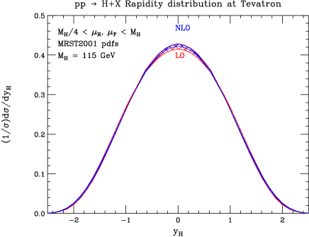
Figure 2: CP even Higgs boson rapidity distribution at the Tevatron at leading (red) and next-to-leading order (blue) in perturbative QCD.

5 Summary

In this paper we computed the NLO rapidity distribution of CP-even and CP-odd Higgs bosons produced at hadron colliders. We found that the NLO corrections change the rapidity distribution, normalized to the total hadronic cross section, only by a small amount. For example, at zero rapidity the NLO normalized distribution for the LHC increases by approximately $5\%$ as compared to LO. The scale variation decreases by a factor of two, from LO to NLO.

The phase-space integrations of the real radiation graphs with fixed rapidity of the Higgs boson are straightforward at this order in perturbation theory. However, traditional methods are very cumbersome for the evaluation of the Higgs boson rapidity distributions at NNLO. In this paper, we performed the first test of the extension of the method suggested in Ref. [2] for evaluating phase-space integrals using multiloop techniques, by applying it to the rapidity distribution of a hadroproduced color-singlet state.

We are confident that the same method is tractable for the evaluation of the differential distributions in more complicated cases, such as the rapidity distribution for Drell-Yan and Higgs boson hadroproduction at NNLO. This will be the subject of a future work.

References

- [1] A. Djouadi, M. Spira, and P. M. Zerwas, Phys. Lett. B264, 440 (1991); S. Dawson, Nucl. Phys. B359, 283 (1991); D. Graudenz, M. Spira, and P. M. Zerwas, Phys. Rev. Lett. 70, 1372 (1993); M. Spira, A. Djouadi, D. Graudenz, and P. M. Zerwas, Nucl. Phys. B453, 17 (1995).
- [2] C. Anastasiou and K. Melnikov, Nucl. Phys. B646, 220 (2002).
- [3] C. Anastasiou and K. Melnikov, arXiv:hep-ph/0208115; R. V. Harlander and W. B. Kilgore, JHEP 0210, 017 (2002); R. V. Harlander and W. B. Kilgore, Phys. Rev. Lett. 88, 201801 (2002); S. Catani, D. de Florian, and M. Grazzini, JHEP 0201, 015 (2002); R. V. Harlander and W. B. Kilgore, Phys. Rev. D64, 013015 (2001).
- [4] D. de Florian, M. Grazzini, and Z. Kunszt, Phys. Rev. Lett. 82, 5209 (1999).
- [5] V. Ravindran, J. Smith, and W. L. Van Neerven, Nucl. Phys. B634, 247 (2002); C. J. Glosser and C. R. Schmidt, arXiv:hep-ph/0209248; E. L. Berger and J.-W. Qiu, arXiv:hep-ph/0210135.
- [6] B. Field, J. Smith, M. E. Tejeda-Yeomans and W. L. van Neerven, arXiv:hep-ph/0210369.
- [7] Z. Bern, L. Dixon and C. Schmidt, Phys. Rev. D66, 074018 (2002).
- [8] S. Catani and M. H. Seymour, Nucl. Phys. B485, 291 (1997).
- [9] K. G. Chetyrkin, B. A. Kniehl, and M. Steinhauser, Phys. Rev. Lett. 79, 2184 (1997); K. G. Chetyrkin, B. A. Kniehl, and M. Steinhauser, Nucl. Phys. B510, 61 (1998); K. G. Chetyrkin, B. A. Kniehl, M. Steinhauser, and W. A. Bardeen, Nucl. Phys. B535, 3 (1998).
- [10] G. Altarelli, R. K. Ellis and G. Martinelli, Nucl. Phys. B157, 461 (1979).
-
[11]
F.V. Tkachov,
Phys. Lett. B100, 65 (1981);
K.G. Chetyrkin and F.V. Tkachov, Nucl. Phys. B192, 159 (1981).