Study of CP Property of the Higgs at a Photon Collider using $\gamma\gamma\rightarrow t\bar{t}\rightarrow lX$

Abstract

We study possible effects of CP violation in the Higgs sector on $t\bar{t}$ production at a $\gamma\gamma$-collider. These studies are performed in a model-independent way in terms of six form-factors $\{\Re(S_{\gamma}),\Im(S_{\gamma}),\Re(P_{\gamma}),\Im(P_{\gamma}),S_{t},P_{t}\}$ which parametrize the CP mixing in the Higgs sector, and a strategy for their determination is developed. We observe that the angular distribution of the decay lepton from $t/\bar{t}$ produced in this process is independent of any CP violation in the $tbW$ vertex and hence best suited for studying CP mixing in the Higgs sector. Analytical expressions are obtained for the angular distribution of leptons in the c.m. frame of the two colliding photons for a general polarization state of the incoming photons. We construct combined asymmetries in the initial state lepton (photon) polarization and the final state lepton charge. They involve CP even ($x$’s) and odd ($y$’s) combinations of the mixing parameters. We study limits up to which the values of $x$ and $y$, with only two of them allowed to vary at a time, can be probed by measurements of these asymmetries, using circularly polarized photons. We use the numerical values of the asymmetries predicted by various models to discriminate among them. We show that this method can be sensitive to the loop-induced CP violation in the Higgs sector in the MSSM.

I Introduction

The Standard Model (SM) has been tested to an extremely high degree of accuracy, reaching its high point in the precision measurements at LEP. However, the bosonic sector of the SM in not yet complete, the Higgs boson is yet to be found. A direct experimental demonstration of the Higgs mechanism of the fermion mass generation still does not exist. Also lacking is a first principle understanding of CP violation in the SM. In this note we look at the possibilities of probing potential CP violation in the Higgs sector at the proposed $\gamma\gamma$ colliders tdr .

Such a study necessarily means that we are looking at models with an extended Higgs sector. CP violation in the Higgs sector can be either explicit, one of the first formulations of such a CP violation being the Weinberg Model weinberg , or can be spontaneous tdlee , where the vacuum becomes CP non-invariant. The mechanism for creating CP violation in the Higgs sector could be different in different models but all such mechanisms will result in CP mixing and then the mass eigenstate scalar will have no definite CP transformation property. In specific models with an extended Higgs sector, such as the Minimal Supersymmetric Standard Model (MSSM), for example, the lightest Higgs remains more or less a CP eigenstate and the two heavier states $H,A$, which would be CP-even and CP-odd respectively in the absence of CP violation and are close in mass to each other, mix. The expected mixing can actually be calculated as a function of the various parameters of the model mssmpaper ; asak1 ; newmssm . In our study, however, we do not stick to a particular model of CP violation and adopt a model-independent approach to study the effects of this CP violation on $t\bar{t}$ production in $\gamma\gamma$ collisions. Such an approach has been adopted in earlier studies asakawa .

We study $\gamma\gamma\rightarrow t\bar{t}$ through the diagrams shown in Fig. 1. It has been observed earlier asakawa that there exists a polarization asymmetry of the $t\bar{t}$ produced in the final state if the scalar $\phi$ exchanged in the $s$-channel is not a CP eigenstate. We parametrize the ${\cal V}_{\gamma\gamma\phi},{\cal V}_{t\bar{t}\phi}$ vertices in a model-independent way in terms of six form factors to include the CP mixing, following Ref. asakawa . We investigate in this study the effect of such a CP mixing on the angular and charge asymmetries for the decay leptons coming from the $t/\bar{t}$ which reflect the top polarization asymmetries. It is known gunion that $\gamma\gamma$ colliders can provide crucial information on the CP property of the scalar produced in the $s$-channel, due to the very striking dependence of the process on the polarization of the $\gamma$’s. These colliders will also offer the possibility of measuring the two-photon width of the SM Higgs very accurately sm2gh ; maria . The $\gamma\gamma$ production of a scalar followed by its decay into a $Z$ pair is shown to provide crucial information required for a model independent confirmation of its spin and parity zerwasnew . Possibilities of studying the MSSM Higgs bosons in $\gamma\gamma$ collisions in the $b\bar{b}$ and neutralino-pair final states, are shown zerwas to give access to regions of the supersymmetric parameter space not accessible at other colliders. Thus in general the $\gamma\gamma$ colliders will provide a very good laboratory for studying the scalar sector. Here we concentrate on the polarization asymmetries of the final state $t$ and $\bar{t}$ caused by such a CP violation asakawa . The large mass of $t$ implies that it decays before hadronization. As a result it acts as a heavy lepton and the spin information gets translated to distribution of the decay leptons. Thus we can use these angular distributions as a probe for possible CP violation. We use only the decay lepton angular distributions and construct asymmetries that reflect the $t/\bar{t}$ polarization asymmetries caused by the CP violation in the Higgs couplings. We observe that these are independent of any CP-violating contribution in the $tbW$ vertex. The same is not true of the energy distribution of the decay lepton. Hence we restrict our analysis to the angular distributions and keep the $tbW$ vertex completely general, choosing the $t\bar{t}\gamma$ vertex

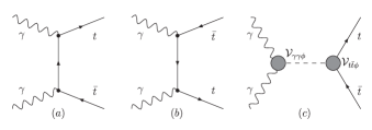
Figure 1: Feynman diagrams contributing to $\gamma\gamma\rightarrow t\bar{t}$ production.

to be standard. The latter of course is relevant only for the continuum background.

We develop a strategy to study the CP property of the Higgs by looking at angular distributions of leptons and antileptons, for different polarizations of the colliding photons. Towards this end we obtain analytical expressions for the lepton angular distribution, with a fixed value of the photon energy and general polarization. We then fold this expression with the photon luminosity function and the polarization profile for the ideal back-scattered laser spectrum ginzburg ; we obtain numerical results for the different mixed polarisation and charge asymmetries which we construct. Our choice of the ideal case for the back-scattered laser spectrum is for demonstration purposes. Further results using the recently available spectra, including the detector simulation for TESLA zarnecki ; telnov12 , will be presented elsewhere usfuture . We then use the above-mentioned asymmetries to assess the sensitivity of this process to the size of various form factors involved in the parametrization of ${\cal V}_{\gamma\gamma\phi},{\cal V}_{t\bar{t}\phi}$. At times we have used specific predictions for the form factors in the MSSM asakawa as a guide and for purposes of illustration, in our analysis. We show that this process is capable of probing the MSSM loop effects using these asymmetries.

The plan of the paper is as follows. In section II we give the general form for CP-violating vertices involving the Higgs, the $t$ quark and the photons as well as the $tbW$ decay vertex for the $t$ quark. The $t\bar{t}$ production and $t$-decay helicity amplitudes obtained with these vertices are then presented. In section III we obtain an analytic expression for the angular distribution of the decay lepton in $t/\bar{t}$ decay. We discuss the insensitivity of the decay-lepton angular distribution to the anomalous coupling in the $tbW$ vertex. Section IV deals with the ideal photon collider ginzburg . Numerical results are presented in section V, discussed in section VI and we conclude in section VII.

II Interaction Vertices and          Helicity Amplitudes

The interaction vertex of $t$ with a scalar $\phi$, which may or may not be a CP eigenstate, may be written in a model-independent way as

$${\cal V}_{t\bar{t}\phi}=-ie\frac{m_{t}}{M_{W}}\left(S_{t}+i\gamma^{5}P_{t}\right).$$ (1)

The general expression for the loop-induced $\gamma\gamma\phi$ vertex can be parametrized as

$${\cal V}_{\gamma\gamma\phi}=\frac{-i\sqrt{s}\alpha}{4\pi}\left[S_{\gamma}(s)\left(\epsilon_{1}.\epsilon_{2}-\frac{2}{s}(\epsilon_{1}.k_{2})(\epsilon_{2}.k_{1})\right)\right.$$

$$-\left.P_{\gamma}(s)\frac{2}{s}\epsilon_{\mu\nu\alpha\beta}\epsilon_{1}^{\mu}\epsilon_{2}^{\nu}k_{1}^{\alpha}k_{2}^{\beta}\right],$$ (2)

where $k_{1}$ and $k_{2}$ are the four-momenta of colliding photons and $\epsilon_{1,2}$ are corresponding polarization vectors. We take $S_{\gamma},P_{\gamma}$ to be complex whereas $S_{t},P_{t}$ are taken to be real. This choice means that we assume only the CP mixing coming from the loop-induced effects in the Higgs potential. We allow these form factors to be slowly varying functions of the $\gamma\gamma$ c.m. energy since in any model the loop-induced couplings will have such a dependence. Simultaneous non-zero values for $P$ and $S$ form factors signal CP violation. We will construct various asymmetries which can give information on these form factors.

We allow the $tbW$ vertex to be completely general and write it as

$$\Gamma^{\mu}_{tbW}=-\frac{g}{\sqrt{2}}V_{tb}\left[\gamma^{\mu}\left(f_{1L}P_{L}+f_{1R}P_{R}\right)\right.$$

$$-\left.\frac{i}{M_{W}}\sigma^{\mu\nu}(p_{t}-p_{b})_{\nu}\left(f_{2L}P_{L}+f_{2R}P_{R}\right)\right],$$ (3)

$${\bar{\Gamma}}^{\mu}_{\bar{t}\bar{b}W}=-\frac{g}{\sqrt{2}}V_{tb}^{*}\left[\gamma^{\mu}\left({\bar{f}}_{1L}P_{L}+{\bar{f}}_{1R}P_{R}\right)\right.$$

$$-\left.\frac{i}{M_{W}}\sigma^{\mu\nu}(p_{\bar{t}}-p_{\bar{b}})_{\nu}\left({\bar{f}}_{2L}P_{L}+{\bar{f}}_{2R}P_{R}\right)\right],$$ (4)

where $V_{tb}$ is the CKM matrix element and $g$ is the $SU(2)$ coupling. We work in the approximation of vanishing $b$ mass. Hence $f_{1R},{\bar{f}}_{1R},f_{2L}$ and ${\bar{f}}_{2R}$ do not contribute. We choose SM values for $f_{1L}$, and ${\bar{f}}_{1L}$, viz., $f_{1L}={\bar{f}}_{1L}=1$. The only non-standard part of the $tbW$ vertex which gives non-zero contribution then corresponds to the terms with $f_{2R}$ and ${\bar{f}}_{2L}$. We will sometimes also use the notation $f^{+}$ and $f^{-}$ for $f_{2R}$ and $\bar{f}_{2L}$ respectively. One expects these unknown $f$’s to be small and we retain only linear terms in them while calculating the amplitudes. Below we give the helicity amplitudes for the production of $t\bar{t}$ followed by the decays of the $t/\bar{t}$ in terms of these general couplings.

II.1 Production Helicity Amplitude

The production process $\gamma\gamma\rightarrow t\bar{t}$ receives the $t/u$ channel SM contribution from the first two diagrams of Fig. 1, which is CP-conserving whereas the $s$ channel $\phi$ exchange contribution may be potentially CP violating. The helicity amplitudes for the $s$ and the $t/u$ channel diagrams are given by Eqs. (5) and (6) respectively :

$$M_{\phi}(\lambda_{1},\lambda_{2};\lambda_{t},\lambda_{\bar{t}})=\frac{-ie\alpha m_{t}}{4\pi M_{W}}\ \frac{s}{s-m_{\phi}^{2}+im_{\phi}\Gamma_{\phi}}$$

$$\left[S_{\gamma}(s)+i\lambda_{1}P_{\gamma}(s)\right]\left[\lambda_{t}\beta S_{t}-iP_{t}\right]\ \delta_{\lambda_{1},\lambda_{2}}\delta_{\lambda_{t},\lambda_{\bar{t}}},$$ (5)

$$M_{SM}(\lambda_{1},\lambda_{2};\lambda_{t},\lambda_{\bar{t}})=\frac{-i4\pi\alpha Q^{2}}{1-\beta^{2}\cos^{2}\theta_{t}}$$

$$\left[\frac{4m_{t}}{\sqrt{s}}\ (\lambda_{1}+\lambda_{t}\beta)\ \delta_{\lambda_{1},\lambda_{2}}\delta_{\lambda_{t},\lambda_{\bar{t}}}\right.$$

$$-\frac{4m_{t}}{\sqrt{s}}\ \lambda_{t}\beta\sin^{2}\theta_{t}\ \delta_{\lambda_{1},-\lambda_{2}}\delta_{\lambda_{t},\lambda_{\bar{t}}}$$

$$-\left.2\beta\ (\cos\theta_{t}+\lambda_{1}\lambda_{t})\sin\theta_{t}\ \delta_{\lambda_{1},-\lambda_{2}}\delta_{\lambda_{t},-\lambda_{\bar{t}}}\right].$$ (6)

Here $\beta,\ Q$ and $\theta_{t}$ are velocity, electric charge and scattering angle of the $t$ quark respectively; $\Gamma_{\phi}$ and $m_{\phi}$ denote the total decay width and mass of the scalar $\phi$; $\lambda_{1,2}$ stand for helicities of two photons while the other $\lambda$’s stand for helicities of particles indicated by the subscript. For photons, helicities are written in units of $\hbar$ while for spin-1/2 fermions they are in units of $\hbar/2$.

From the expressions in Eqs. (5) and (6) it is clear that the $\phi$ exchange diagram contributes only when both colliding photons have the same helicities, whereas the SM contribution is small for this combination as we move away from the $t\bar{t}$ threshold. Thus a choice of equal helicities for both colliding photons can maximize polarization asymmetries for the produced $t\bar{t}$ pair, better reflecting the CP-violating nature of the $s$-channel contribution. It should be mentioned here that these statements are true only in the leading order (LO). Radiative corrections to $\gamma\gamma\rightarrow q\bar{q}$ can be large jikia ; melles . That is also the reason we have restricted our analysis to asymmetries, which involve ratios. As a result the analysis is quite robust even if we use only the LO result for the SM contribution. Note also that the SM contribution for equal photon helicities is peaked in the forward and backward directions, whereas the scalar-exchange contribution is independent of the production angle $\theta_{t}$. This also suggests that one can optimize the asymmetries by angular cuts to reduce the SM contributions to the integrated cross-section, of course taking care that the total event rate is not reduced too much. We will make use of this feature in our studies.

II.2 Decay Helicity Amplitudes

We assume that the $t$ quark decays only via the $tbW$ vertex followed by the decay of $W$ into lepton and corresponding neutrino. The helicity amplitudes $M_{\Gamma}(\lambda_{t},\lambda_{b},\lambda_{l^{+}},\lambda_{\nu})$ and $\overline{M}_{\Gamma}(\lambda_{\bar{t}},\lambda_{\bar{b}},\lambda_{l^{-}},\lambda_{\bar{\nu}})$, for the decay of $t$ and $\bar{t}$ are given below:

$$M_{\Gamma}(+,-,+,-)=-i2\sqrt{2}g^{2}\sqrt{m_{t}p^{0}_{b}p^{0}_{\nu}p^{0}_{l^{+}}}\ \Delta_{W}(p_{W}^{2})$$

$$\times\left\{\left(1+\frac{f_{2R}}{\sqrt{r}}\right)\cos\frac{\theta_{l^{+}}}{2}\left[\cos\frac{\theta_{\nu}}{2}\sin\frac{\theta_{b}}{2}e^{i\phi_{b}}-\right.\right.$$

$$\left.\sin\frac{\theta_{\nu}}{2}\cos\frac{\theta_{b}}{2}e^{i\phi_{\nu}}\right]-\frac{f_{2R}}{\sqrt{r}}\sin\frac{\theta_{b}}{2}e^{i\phi_{b}}$$

$$\left.\left[\sin\frac{\theta_{\nu}}{2}\sin\frac{\theta_{l^{+}}}{2}e^{i(\phi_{\nu}-\phi_{l^{+}})}+\cos\frac{\theta_{\nu}}{2}\cos\frac{\theta_{l^{+}}}{2}\right]\right\},$$ (7)

$$M_{\Gamma}(-,-,+,-)=-i2\sqrt{2}g^{2}\sqrt{m_{t}p^{0}_{b}p^{0}_{\nu}p^{0}_{l^{+}}}\ \Delta_{W}(p_{W}^{2})$$

$$\times\left\{\left(1+\frac{f_{2R}}{\sqrt{r}}\right)\sin\frac{\theta_{l^{+}}}{2}e^{-i\phi_{l^{+}}}\left[\cos\frac{\theta_{\nu}}{2}\sin\frac{\theta_{b}}{2}e^{i\phi_{b}}\right.\right.$$

$$-\left.\sin\frac{\theta_{\nu}}{2}\cos\frac{\theta_{b}}{2}e^{i\phi_{n}}\right]+\frac{f_{2R}}{\sqrt{r}}\cos\frac{\theta_{b}}{2}$$

$$\left.\left[\sin\frac{\theta_{\nu}}{2}\sin\frac{\theta_{l^{+}}}{2}e^{i(\phi_{\nu}-\phi_{l^{+}})}+\cos\frac{\theta_{\nu}}{2}\cos\frac{\theta_{l^{+}}}{2}\right]\right\},$$ (8)

$$\overline{M}_{\Gamma}(+,+,-,+)=-i2\sqrt{2}g^{2}\sqrt{m_{t}p^{0}_{\bar{b}}p^{0}_{\bar{\nu}}p^{0}_{l^{-}}}\ \Delta_{W}(p_{W}^{2})$$

$$\times\left\{\left(1+\frac{\bar{f}_{2L}}{\sqrt{r}}\right)\cos\frac{\theta_{l^{-}}}{2}\left[\cos\frac{\theta_{\bar{\nu}}}{2}\sin\frac{\theta_{\bar{b}}}{2}e^{-i\phi_{\bar{b}}}\right.\right.$$

$$-\left.\sin\frac{\theta_{\bar{\nu}}}{2}\cos\frac{\theta_{\bar{b}}}{2}e^{-i\phi_{\bar{\nu}}}\right]-\frac{\bar{f}_{2L}}{\sqrt{r}}\sin\frac{\theta_{\bar{b}}}{2}e^{-i\phi_{\bar{b}}}$$

$$\left.\left[\sin\frac{\theta_{\bar{\nu}}}{2}\sin\frac{\theta_{l^{-}}}{2}e^{-i(\phi_{\bar{\nu}}-\phi_{l^{-}})}+\cos\frac{\theta_{\bar{\nu}}}{2}\cos\frac{\theta_{l^{-}}}{2}\right]\right\},$$ (9)

$$\overline{M}_{\Gamma}(-,+,-,+)=-i2\sqrt{2}g^{2}\sqrt{m_{t}p^{0}_{\bar{b}}p^{0}_{\bar{\nu}}p^{0}_{l^{-}}}\ \Delta_{W}(p_{W}^{2})$$

$$\times\left\{\left(1+\frac{\bar{f}_{2L}}{\sqrt{r}}\right)\sin\frac{\theta_{l^{-}}}{2}e^{i\phi_{l^{-}}}\left[\cos\frac{\theta_{\bar{\nu}}}{2}\sin\frac{\theta_{\bar{b}}}{2}e^{-i\phi_{\bar{b}}}\right.\right.$$

$$-\left.\sin\frac{\theta_{\bar{\nu}}}{2}\cos\frac{\theta_{\bar{b}}}{2}e^{-i\phi_{\bar{\nu}}}\right]+\frac{\bar{f}_{2L}}{\sqrt{r}}\cos\frac{\theta_{\bar{b}}}{2}$$

$$\left.\left[\sin\frac{\theta_{\bar{\nu}}}{2}\sin\frac{\theta_{l^{-}}}{2}e^{-i(\phi_{\bar{\nu}}-\phi_{l^{-}})}+\cos\frac{\theta_{\bar{\nu}}}{2}\cos\frac{\theta_{l^{-}}}{2}\right]\right\},$$ (10)

where,

$$\Delta_{W}(p_{W}^{2})\ =\ \frac{1}{p_{W}^{2}-M_{W}^{2}+iM_{W}\Gamma_{W}},\hskip 5.69046ptr=\frac{M_{W}^{2}}{m_{t}^{2}}.$$

For simplicity, the above expressions for the decay amplitudes have been calculated in the rest frame of $t$ ($\bar{t}$) with the $z$-axis pointing in the direction of its momentum in the $\gamma\gamma$ c.m. frame. We treat the decay lepton $l$ and the $b$ quark as massless and list only the non-zero amplitudes.

III Angular Distribution of Leptons

Using the narrow-width approximation for the $t$ quark and the $W$ boson, the differential cross section for $\gamma\gamma\rightarrow t\bar{t}\rightarrow l^{+}b\nu_{l}\bar{t}$ can be written in terms of the density matrices as

$$\frac{d\sigma}{d\cos\theta_{t}\ d\cos\theta_{l^{+}}\ dE_{l^{+}}\ d\phi_{l^{+}}}=\frac{3e^{4}g^{4}\beta E_{l^{+}}}{64(4\pi)^{4}s\Gamma_{t}m_{t}\Gamma_{W}M_{W}}$$

$$\ \sum_{\lambda,\lambda^{\prime}}\underbrace{\rho^{{}^{\prime}+}(\lambda,\lambda^{\prime})}_{\rm c.m.\ frame}\underbrace{\left[\frac{\Gamma^{\prime}(\lambda,\lambda^{\prime})}{m_{t}E_{l^{+}}^{0}}\right]}_{\rm rest\ frame}.$$

(11)

Here $E_{l^{+}}^{0}$ is the energy of $l^{+}$ in the rest frame of the $t$ quark; the production and decay density matrices are given by

$$\rho^{+}(\lambda,\lambda^{\prime}) = e^{4}\rho^{{}^{\prime}+}(\lambda,\lambda^{\prime})=\sum\rho_{1}(\lambda_{1},\lambda_{1}^{\prime})\rho_{2}(\lambda_{2},\lambda_{2}^{\prime})$$

$$\times\ {\cal M}(\lambda_{1},\lambda_{2},\lambda,\lambda_{\bar{t}}){\cal M}^{*}(\lambda_{1}^{\prime},\lambda_{2}^{\prime},\lambda^{\prime},\lambda_{\bar{t}})$$

$${\rm and}$$

$$\Gamma(\lambda,\lambda^{\prime}) = g^{4}|\Delta(p_{W}^{2})|^{2}\ \Gamma^{\prime}(\lambda,\lambda^{\prime})=\frac{1}{2\pi}\int d\alpha$$

$$\times\sum M_{\Gamma}(\lambda,\lambda_{b},\lambda_{l^{+}},\lambda_{\nu})\ M_{\Gamma}^{*}(\lambda^{\prime},\lambda_{b},\lambda_{l^{+}},\lambda_{\nu}).$$

Here $\alpha$ is the azimuthal angle of the $b$ quark in the rest frame of the $t$ quark with the $z$-axis pointing in the direction of the momentum of the lepton. All repeated indices of matrix elements and density matrices are summed over; $\rho_{1(2)}$ are the photon density matrices; written, in terms of the Stokes parameters $\eta_{i},\xi_{i}$:

$$\rho_{1}(\lambda_{1},\lambda_{1}^{\prime})=\frac{1}{2}\left[\begin{tabular}[]{cc}$1+\eta_{2}$&$-\eta_{3}+i\eta_{1}$\\ $-\eta_{3}-i\eta_{1}$&$1-\eta_{2}$\end{tabular}\right],$$ (14)

$$\rho_{2}(\lambda_{2},\lambda_{2}^{\prime})=\frac{1}{2}\left[\begin{tabular}[]{cc}$1+\xi_{2}$&$-\xi_{3}+i\xi_{1}$\\ $-\xi_{3}-i\xi_{1}$&$1-\xi_{2}$\end{tabular}\right].$$ (17)

Here, $\eta_{2}$ is the degree of circular polarization while $\eta_{1}$ and $\eta_{3}$ are degrees of linear polarizations in two transverse directions of one photon; $\xi_{i}$ are similarly the degrees of polarization for the second photon. The explicit expressions for the production density matrix $\rho(\lambda_{t},\lambda_{t}^{\prime})$ depend upon the polarization of initial photons. The decay density matrix elements are independent of any initial condition and in the rest frame of $t$ ($\bar{t}$) they are given by:

$$\Gamma(\pm,\pm)=g^{4}m_{t}E_{l^{+}}^{0}|\Delta_{W}(p_{W}^{2})|^{2}\ (m_{t}^{2}-2p_{t}.p_{l^{+}})$$

$$(1\pm\cos\theta_{l^{+}})\left(1+\frac{\Re(f_{2R})}{\sqrt{r}}\frac{M_{W}^{2}}{p_{t}.p_{l^{+}}}\right),$$ (18)

$$\Gamma(\pm,\mp)=g^{4}m_{t}E_{l^{+}}^{0}|\Delta_{W}(p_{W}^{2})|^{2}\ (m_{t}^{2}-2p_{t}.p_{l^{+}})$$

$$\sin\theta_{l^{+}}e^{\pm i\phi_{l^{+}}}\left(1+\frac{\Re(f_{2R})}{\sqrt{r}}\frac{M_{W}^{2}}{p_{t}.p_{l^{+}}}\right),$$ (19)

$$\overline{\Gamma}(\pm,\pm)=g^{4}m_{t}E_{l^{-}}^{0}|\Delta_{W}(p_{W}^{2})|^{2}\ (m_{t}^{2}-2p_{\bar{t}}.p_{l^{-}})$$

$$(1\pm\cos\theta_{l^{-}})\left(1+\frac{\Re(\bar{f}_{2L})}{\sqrt{r}}\frac{M_{W}^{2}}{p_{\bar{t}}.p_{l^{-}}}\right),$$ (20)

$$\overline{\Gamma}(\pm,\mp)=g^{4}m_{t}E_{l^{-}}^{0}|\Delta_{W}(p_{W}^{2})|^{2}\ (m_{t}^{2}-2p_{\bar{t}}.p_{l^{-}})$$

$$\sin\theta_{l^{-}}e^{\mp i\phi_{l^{-}}}\left(1+\frac{\Re(\bar{f}_{2L})}{\sqrt{r}}\frac{M_{W}^{2}}{p_{\bar{t}}.p_{l^{-}}}\right).$$ (21)

We have kept only the linear terms in the form factors $f_{2R}$ and $\bar{f}_{2L}$, as we assume them to be small. These expressions written in terms of the lab variables can also be written in terms of the variables in the $\gamma\gamma$ c.m. frame. The relations between the angles in the rest frame and the $\gamma\gamma$ c.m. frame can be easily derived and are given by

$$1\pm\cos\theta_{l^{+}}=\frac{(1\mp\beta)(1\pm\cos\theta_{tl^{+}}^{c.m.})}{1-\beta\cos\theta_{tl^{+}}^{c.m.}},$$ (22)

$$1\pm\cos\theta_{l^{-}}=\frac{(1\pm\beta)(1\mp\cos\theta_{\bar{t}l^{-}}^{c.m.})}{1-\beta\cos\theta_{\bar{t}l^{-}}^{c.m.}},$$ (23)

$$\sin\theta_{l^{+}}e^{i\phi_{l^{+}}}=\frac{\sqrt{1-\beta^{2}}}{1-\beta\cos\theta_{tl^{+}}^{c.m.}}$$

$$(\sin\theta_{l^{+}}^{c.m.}\cos\theta_{t}^{c.m.}\cos\phi_{l^{+}}^{c.m.}-\cos\theta_{l^{+}}^{c.m.}\sin\theta_{t}^{c.m.}$$

$$+i\sin\theta_{l^{+}}^{c.m.}\sin\phi_{l^{+}}^{c.m.}),$$ (24)

$$\sin\theta_{l^{-}}e^{i\phi_{l^{-}}}=\frac{\sqrt{1-\beta^{2}}}{1-\beta\cos\theta_{\bar{t}l^{-}}^{c.m.}}$$

$$(-\sin\theta_{l^{-}}^{c.m.}\cos\theta_{\bar{t}}^{c.m.}\cos\phi_{l^{-}}^{c.m.}+\cos\theta_{l^{-}}^{c.m.}\sin\theta_{\bar{t}}^{c.m.}$$

$$+i\sin\theta_{l^{-}}^{c.m.}\sin\phi_{l^{-}}^{c.m.}).$$ (25)

Using the above relations and dropping the superscripts c.m. from the angles, we can rewrite Eq. (11) as

$$\frac{d\sigma}{d\cos\theta_{t}d\cos\theta_{l^{\pm}}dE_{l^{\pm}}d\phi_{l^{\pm}}}=\frac{3\alpha^{4}\beta}{16x_{w}^{2}\sqrt{s}}\frac{E_{l^{\pm}}}{\Gamma_{t}\Gamma_{W}M_{W}}$$

$$\frac{1}{8\gamma_{t}}\left(\frac{1}{1-\beta\cos\theta_{tl}}-\frac{4E_{l^{\pm}}}{\sqrt{s}(1-\beta^{2})}\right)$$

$$\times\left(1+\frac{\Re(f^{\pm})}{\sqrt{r}}\frac{2M_{W}^{2}}{E_{l^{\pm}}\sqrt{s}(1-\beta\cos\theta_{tl})}\right)$$

$$\times\left[A^{\pm}(1-\beta\cos\theta_{tl})\pm B^{\pm}(\cos\theta_{tl}-\beta)\right.$$

$$\pm C^{\pm}\sqrt{1-\beta^{2}}\sin\theta_{l^{\pm}}(\cos\theta_{t}\cos\phi_{l^{\pm}}-\sin\theta_{t}\cot\theta_{l^{\pm}})$$

$$\left.\pm D^{\pm}\sqrt{1-\beta^{2}}\sin\theta_{l^{\pm}}\sin\phi_{l^{\pm}}\right],$$ (26)

where $\gamma_{t}=1/\sqrt{1-\beta^{2}}$, $x_{w}=\sin^{2}\theta_{W}$, $\theta_{W}$ being the Weinberg angle and

$$A^{\pm} = \rho^{{}^{\prime}\pm}(+,+)+\rho^{{}^{\prime}\pm}(-,-),$$ (27)

$$B^{\pm} = \rho^{{}^{\prime}\pm}(+,+)-\rho^{{}^{\prime}\pm}(-,-),$$ (28)

$$C^{\pm} = 2\Re[\rho^{{}^{\prime}\pm}(+,-)],$$ (29)

$$D^{\pm} = -2\Im[\rho^{{}^{\prime}\pm}(+,-)].$$ (30)

In Eq. (26) and what follows, the lepton variables are defined in the $\gamma\gamma$ c.m. frame. Further, $\theta_{tl}$ stands for $\theta_{tl^{+}}$ for the $l^{+}$ distribution and hence the upper sign in the equation, whereas it stands for $\theta_{\bar{t}l^{-}}$ for the lower sign and hence the $l^{-}$ distribution. To get the angular distribution of leptons we still have to integrate Eq. (26) over $E_{l},\ \cos\theta_{t}$ and $\phi_{l}$. The limits on $E_{l}$ integration are,

$$\frac{M_{W}^{2}}{\sqrt{s}}\ \frac{1}{1-\beta\cos\theta_{tl}}\ \leq\ E_{l}\ \leq\frac{m_{t}^{2}}{\sqrt{s}}\ \frac{1}{1-\beta\cos\theta_{tl}}.$$

After the $E_{l}$ integration, we get

$$\frac{d\sigma}{d\cos\theta_{t}\ d\cos\theta_{l^{\pm}}\ d\phi_{l^{\pm}}}=\frac{3\alpha^{4}\beta}{16x_{w}^{2}\sqrt{s}}\ \frac{1}{\Gamma_{t}\Gamma_{W}M_{W}}$$

$$\frac{1}{8\gamma_{t}}\ \frac{m_{t}^{4}}{6s}\ \frac{(1+2r-6\Re(f^{\pm})\sqrt{r})(1-r)^{2}}{(1-\beta\cos\theta_{tl})^{3}}$$

$$\times\left[A^{\pm}(1-\beta\cos\theta_{tl})\pm B^{\pm}(\cos\theta_{tl}-\beta)\right.$$

$$\pm C^{\pm}\sqrt{1-\beta^{2}}\sin\theta_{l^{\pm}}(\cos\theta_{t}\cos\phi_{l^{\pm}}-\sin\theta_{t}\cot\theta_{l^{\pm}})$$

$$\left.\pm D^{\pm}\sqrt{1-\beta^{2}}\sin\theta_{l^{\pm}}\sin\phi_{l^{\pm}}\right].$$ (31)

Here we have used the notation $f^{+}$ and $f^{-}$ for $f_{2R}$ and $\bar{f}_{2L}$, respectively. From the above equation it is clear that the angular distribution of leptons after energy integration is modified due to the anomalous $tbW$ coupling only up to an overall factor $1+2r-6\Re(f^{\pm})\sqrt{r}$, which is independent of any kinematical variable. In fact, the same factor appears in the total width of the $t$ quark calculated up to linear order in $f^{\pm}$:

$$\Gamma_{t(\bar{t})}=\frac{\alpha^{2}}{192x_{w}^{2}}\frac{m_{t}^{3}}{\Gamma_{W}M_{W}}(1-r)^{2}\left[1+2r-6\Re(f^{\pm})\sqrt{r}\right]$$ (32)

and thus exactly cancels the one in Eq. (31). Thus we see that the angular distribution of the decay lepton is unaltered, in the linear approximation of anomalous $tbW$ couplings. In fact this is quite a general result, which is attained under certain assumptions and approximations we have made. We elaborate on this point below.

An inspection of Eqs. (18)–(21) shows that the presence of any anomalous part in the $tbW$ coupling changes the decay density matrix only by an overall energy-dependent factor independent of angle. The quantity $p_{t}.p_{l}$ does have an apparent dependence on the angular variables of the lepton. However, in fact it depends only on the lepton energy. To see this clearly, let us go to the rest frame of the $t$ quark. Now the three lepton variables are $\{E_{l}^{\rm rest},\theta_{l}^{\rm rest},\phi_{l}^{\rm rest}\}$ and the anomalous term depends only on $E_{l}^{\rm rest}$. This means that the angular distribution of leptons in the rest frame of the $t$ quark is unaltered by the presence of an anomalous term in $tbW$ coupling, apart from an overall scaling. The angular distribution in any other frame can be obtained from that in the rest frame by a Lorentz boost. Thus the angular distribution of leptons in an arbitrary frame will be the same as that in the absence of the anomalous term, up to some overall factor that depends upon energy and the boost parameters and no angular variables. Of course, it is not very obvious by looking at Eq. (21) that this will indeed happen. But, with a change of variable,

$$E_{l}\rightarrow E_{l}^{\rm rest}=\gamma_{t}E_{l}(1-\beta\cos\theta_{tl}),$$

the additional overall factor becomes

$$1+\frac{\Re(f^{\pm})}{\sqrt{r}}\frac{M_{W}^{2}}{m_{t}E_{l}^{\rm rest}},$$

which is clearly independent of angular variables. After integration over $E_{l}^{\rm rest}$, in the limit $M_{W}^{2}/2m_{t}\leq E_{l}^{\rm rest}\leq m_{t}/2$ we get back Eq. (31). The important point is that in proving the result we did not make any reference to the production density matrix and hence the result is very general and applicable to any $2\rightarrow 2$ process for $t\bar{t}$ pair production provided the following conditions are fulfilled:

• we use the narrow-width approximation for $t$ and $W$,

• $b,\ l,\ \nu$ are taken to be massless,

• the only decay mode of $t$ is $t\rightarrow bW\rightarrow bl\nu$, and

• the anomalous $tbW$ coupling is small enough that one can work to linear approximation in it.

For the case of $e^{+}e^{-}\rightarrow t\bar{t}$ followed by subsequent $t/\bar{t}$ decay, this was observed earlier sdr ; hioki . It was proved recently by two groups independently; for a two-photon initial state by Ohkuma ohk , for an arbitrary two-body initial state in grza and further keeping $m_{b}$ non-zero in grza1 . These derivations use the method developed by Tsai and collaborators tsai for incorporating the production and decay of a massive spin-half particle. Our derivation makes use of helicity amplitudes and provides an independent verification of these results. The result is very crucial for our present work as we now have an observable where the only source of the CP-violating asymmetry will be the production process.

Thus we can analyse the Higgs CP property easily, as long as the anomalous part of the $tbW$ couplings, $f^{\pm}$ is small and the quadratic term can be neglected. If $f^{\pm}$ is not small then we have to keep the quadratic terms in Eqs. (18)-(19) and the decay density matrices to this order are then given by :

$$\Gamma(\pm,\pm)=g^{4}m_{t}E_{l^{+}}^{0}|\Delta_{W}(p_{W}^{2})|^{2}\ (m_{t}^{2}-2p_{t}.p_{l^{+}})$$

$$\left[(1\pm\cos\theta_{l^{+}})\left(1+\frac{\Re(f^{+})}{\sqrt{r}}\frac{M_{W}^{2}}{p_{t}.p_{l^{+}}}\right)\right.$$

$$-|f^{+}|^{2}(1\mp\cos\theta_{l^{+}})\left(1-\frac{m_{t}^{2}+M_{W}^{2}}{2p_{t}.p_{l^{+}}}\right)$$

$$\left.+|f^{+}|^{2}\frac{M_{W}^{4}}{2r(p_{t}.p_{l^{+}})^{2}}\cos\theta_{l^{+}}\right],$$ (33)

$$\Gamma(\pm,\mp)=g^{4}m_{t}E_{l^{+}}^{0}|\Delta_{W}(p_{W}^{2})|^{2}\ (m_{t}^{2}-2p_{t}.p_{l^{+}})$$

$$\sin\theta_{l^{+}}e^{\pm i\phi_{l^{+}}}\left[1+\frac{\Re(f^{+})}{\sqrt{r}}\frac{M_{W}^{2}}{p_{t}.p_{l^{+}}}\right.$$

$$+\left.|f^{+}|^{2}\left(1-\frac{m_{t}^{2}+M_{W}^{2}}{2p_{t}.p_{l^{+}}}+\frac{M_{W}^{4}}{2r(p_{t}.p_{l^{+}})^{2}}\right)\right].$$ (34)

$\overline{\Gamma}(\lambda,\lambda^{\prime})$ will be given by similar expressions. Thus if $f^{\pm}$ are not small they can modify the angular dependence of the decay density matrix in the rest frame of the $t$ quark and hence in any other frame. In that case it will not be trivial to use angular distributions to study the CP property of the production process. In this work we will assume $f^{\pm}$ to be small and will neglect the quadratic terms in Eqs. (33) and (34).

Making the above-mentioned four assumptions, which are very reasonable indeed, we now go on to calculate the final angular distribution by integrating Eq. (31) over $\cos\theta_{t}$ and $\phi_{l}$. We obtain for the angular distribution:

$$\frac{d\sigma}{d\cos\theta_{l^{\pm}}}=\frac{3\pi\alpha^{2}\beta}{8s\gamma_{t}^{2}}\ \left[2A_{00}^{\pm}(I_{300}-\beta yI_{301})\right.$$

$$+2A_{01}^{\pm}(I_{310}-\beta yI_{311})+2A_{02}^{\pm}(I_{320}-\beta yI_{321})$$

$$+2A_{22}^{\pm}(I_{322}-\beta yI_{323})+2A_{42}^{\pm}(I_{324}-\beta yI_{325})$$

$$\pm\frac{B_{01}^{\pm}}{\beta}\{-2(I_{310}-\beta yI_{311})+(1-\beta^{2})\sum_{i=0}^{2}X_{i}I_{51i}\}$$

$$\pm\frac{B_{02}^{\pm}}{\beta}\{-2(I_{320}-\beta yI_{321})+(1-\beta^{2})\sum_{i=0}^{2}X_{i}I_{52i}\}$$

$$\pm\frac{B_{12}^{\pm}}{\beta}\{-2(I_{321}-\beta yI_{322})+(1-\beta^{2})\sum_{i=1}^{3}X_{i}I_{52i}\}$$

$$\pm\frac{B_{32}^{\pm}}{\beta}\{-2(I_{323}-\beta yI_{324})+(1-\beta^{2})\sum_{i=3}^{5}X_{i}I_{52i}\}$$

$$\left.\pm C_{0}\ \sum_{j=0}^{6}\ Y_{j}\ I_{52j}\right],$$ (35)

where

$$I_{ijk}=\intop^{1}_{-1}\frac{d\cos\theta_{t}\cos^{k}\theta_{t}}{[a+(y-\beta\cos\theta_{t})^{2}]^{i/2}(1-\beta^{2}\cos^{2}\theta_{t})^{j}},$$

$a$	=	$(1-\beta^{2})\sin^{2}\theta_{l^{\pm}}$,
$y$	=	$\cos\theta_{l^{\pm}}.$

We have obtained explicit analytical expressions for all $I_{ijk}$ appearing in Eq. (35), which are not listed here. $A_{ij}$ and $B_{ij}$ are coefficients in expansions of the following type:

$$A^{\pm}=\sum_{i,j}\frac{A^{\pm}_{ij}\cos^{i}\theta_{t}}{(1-\beta^{2}\cos^{2}\theta_{t})^{j}}\hskip 28.45274pt{\rm etc.}$$

Expressions for $A_{ij}$’s and $B_{ij}$’s for circular polarization of photons and expressions for $X_{i}$’s, $Y_{j}$’s and $C_{0}$ are given in the appendix. Equation (35) is the angular distribution of leptons for a given $\gamma\gamma$ centre-of-mass energy. In a $\gamma\gamma$-collider constructed using the back-scattered laser beam one will not have monoenergetic photons in the inital state; further, the degree of circular polarization of the photons will depend on its energy. Thus the final observable cross section is to be obtained by folding Eq. (35) with the luminosity function after accounting for the energy dependence of the circular polarization of the photons.

IV Photon Collider

In a $\gamma\gamma$ collider, high energy photons are produced by Compton back-scattering of a laser from high energy $e^{-}$ or $e^{+}$ beam via

$$e^{-}(\lambda_{e^{-}})\ \gamma(\lambda_{l_{1}})\rightarrow e^{-}\ \gamma(\lambda_{1})$$

$$e^{+}(\lambda_{e^{+}})\ \gamma(\lambda_{l_{2}})\rightarrow e^{+}\ \gamma(\lambda_{2}).$$

In this paper we will be using the ideal photon spectrum due to Ginzburg et al. for $x\leq 4.8$. The ideal luminosity (for zero conversion distance) is given by

$$\frac{1}{L_{e^{-}e^{+}}}\frac{dL_{\gamma\gamma}}{dy_{1}dy_{2}}=f(y_{1})f(y_{2}),$$ (36)

where

$$f(y) = \frac{2\pi\alpha^{2}}{\sigma_{c}xm_{e}^{2}}\left[\frac{1}{1-y}+1-y-4r(1-r)\right.$$ (37)

$$- \left.\lambda_{e}\lambda_{l}rx(2r-1)(2-y)\right],$$

$$x = \frac{4E_{b}\omega_{0}}{m_{e}^{2}}=15.3\left(\frac{E_{b}}{\rm TeV}\right)\ \left(\frac{\omega_{0}}{\rm eV}\right),$$ (38)

$$r = \frac{y}{x(1-y)}\leq 1,$$ (39)

$$y = \frac{\omega}{E_{b}},\hskip 56.9055pt\omega\leq\frac{xE_{b}}{1+x},$$ (40)

$$\sigma_{c} = \sigma_{c}^{np}+\lambda_{e}\lambda_{l}\sigma_{1},$$ (41)

$$\sigma_{c}^{np} = \frac{2\pi\alpha^{2}}{xm_{e}^{2}}\left[\left(1-\frac{4}{x}-\frac{8}{x^{2}}\right)\log(1+x)\right.$$ (42)

$$+ \left.\frac{1}{2}+\frac{8}{x}-\frac{1}{2(1+x)^{2}}\right],$$

$$\sigma_{1} = \frac{2\pi\alpha^{2}}{xm_{e}^{2}}\left[\left(1+\frac{2}{x}\right)\log(1+x)\right.$$ (43)

$$- \left.\frac{5}{2}+\frac{1}{1+x}-\frac{1}{2(1+x)^{2}}\right],$$

$\lambda_{e}$ and $\lambda_{l}$ are the initial electron (positron) and laser helicities respectively, and $\omega_{0}$ is the energy of the laser. In Eq. (36), if we change variables from $y_{1}$ and $y_{2}$ to $z=\sqrt{y_{1}y_{2}}$ and $y_{2}$ and integrate over $y_{2}$, we will get an expression for the photon spectrum as a function of the $\gamma\gamma$ invariant mass $W=2zE_{b}$, where $E_{b}$ is the energy of the $e^{\pm}$ beam and is plotted in Fig. 2 for $x=4.8$. The spectrum is peaked in the hard photon region for $\lambda_{e}\lambda_{l}=-1$.

The mean helicity of high energy photons depends upon their energy in the

Figure 2: Luminosity distribution plotted against $z$ (which is related to the $\gamma\gamma$ invariant mass $W=2\sqrt{\omega_{1}\omega_{2}}$ by $z=W/(2E_{b})$) for $x=4.8$. Solid line corresponds to $\lambda_{e}\lambda_{l}=-1$, small dashed line is for $\lambda_{e}\lambda_{l}=1$ and large dashed line is for $\lambda_{e}\lambda_{l}=0$. Conversion distance is taken to be zero.

lab frame. In an ideal $\gamma\gamma$ collider the energy dependence of the mean helicity is given by

$$\eta_{2}(y) = \frac{2\pi\alpha^{2}}{\sigma_{c}xm_{e}^{2}f(y)}\left\{\lambda_{l}(1-2r)(1-y+1/(1-y))\right.$$ (44)

$$+\left.\lambda_{e}rx[1+(1-y)(1-2r)^{2}]\right\}$$

and is plotted in Fig. 3 for $x=4.8$.

Figure 3: Mean helicity of scattered high energy photon plotted against reduced energy of photon $y=\omega/E_{b}$. Solid lines are for $\lambda_{e}\lambda_{l}=-1$ and the dashed lines corresponds to $\lambda_{e}\lambda_{l}=1$. The lines are marked with the values of ($\lambda_{e},\lambda_{l}$).

For $\lambda_{e}\lambda_{l}=-1$ the back-scattered photon has the same helicity as the electron (positron). Also, the spectrum is peaked at high energy, and yields a high degree of polarisation of the photon beam. Hence, the dominant photon polarization in this case is decided by the electron (positron) helicity. Now, as suggested by Eq. (5), the helicities of two colliding photons should be equal in order to have Higgs contribution. Thus we choose $\lambda_{e}\lambda_{l}=-1$ to get a hard photon spectrum, and set $\lambda_{e^{-}}=\lambda_{e^{+}}$ to maximize the Higgs contribution, and hence the sensitivity to possible CP-violating interactions. For our numerical analysis, we have chosen $\lambda_{e}\lambda_{l}=-1$; the initial state can thus be completely described by the helicities of the initial electron and positron. We denote the total cross section in the lab frame by $\sigma(\lambda_{e^{-}},\pm)$, where the second argument denotes the charge of the final state lepton.

The total cross-section with an angular cut in the lab frame can be obtained by folding Eq. (35) with the photon spectrum:

$$\sigma(\lambda_{e^{-}},\pm)=\intop\!\!\frac{dL_{\gamma\gamma}}{dy_{1}dy_{2}}dy_{1}dy_{2}\intop_{f(\theta_{0},y_{1},y_{2})}^{g(\theta_{0},y_{1},y_{2})}\!\!\!\!d\cos\theta_{l^{\pm}}\frac{d\sigma}{d\cos\theta_{l^{\pm}}},$$

(45)

where $f(\theta_{0},y_{1},y_{2})$ and $g(\theta_{0},y_{1},y_{2})$ are the (boosted) limits on integration in the $\gamma\gamma$ c.m. frame. We end this section with a few remarks. We have presented the specific case where the $\gamma\gamma$ collider is based on a parent $e^{+}e^{-}$ collider and we also assume $100\%$ polarization for the $e^{-}/e^{+}$. The analysis is completely valid for the case of a parent $e^{-}e^{-}$ collider, for which achieving a high degree of polarization for initial leptons might be technologically simpler.

V Numerical Results

To determine the CP properties of the Higgs, we need to know all the four form factors appearing in Eqs. (1) and (2). Assuming the mass and decay width of Higgs to be known, we then have the following six unknowns

$$S_{t},\ P_{t},\ \Re(S_{\gamma}),\ \Im(S_{\gamma}),\ \Re(P_{\gamma}),\ \Im(P_{\gamma}).$$

They appear in eight combinations in the expression for the production density matrix, which we denote by $x_{i}$ and $y_{i}$ $(i=1,...,4)$, and are listed below, together with their CP properties.

Combinations	Aliases	CP property
$S_{t}\Re(S_{\gamma})$	$x_{1}$	even
$S_{t}\Im(S_{\gamma})$	$x_{2}$	even
$S_{t}\Re(P_{\gamma})$	$y_{1}$	odd
$S_{t}\Im(P_{\gamma})$	$y_{2}$	odd
$P_{t}\Re(S_{\gamma})$	$y_{3}$	odd
$P_{t}\Im(S_{\gamma})$	$y_{4}$	odd
$P_{t}\Re(P_{\gamma})$	$x_{3}$	even
$P_{t}\Im(P_{\gamma})$	$x_{4}$	even

Only five of these combinations are independent because they satisfy the following relations

$$y_{1}\ .\ y_{3}\ =\ x_{1}\ .\ x_{3},\hskip 28.45274pty_{2}\ .\ y_{4}\ =\ x_{2}\ .\ x_{4},$$

$$y_{1}\ .\ x_{4}\ =\ y_{2}\ .\ x_{3},\hskip 28.45274pty_{4}\ .\ x_{1}\ =\ y_{3}\ .\ x_{2}.$$

Any three relations of the four listed above are independent relations while the fourth one is derived. Expressions for asymmetries can by written in terms of $x$’s and $y$’s and can be used to put limits on sizes on these combinations.

In what follows we will define various asymmetries involving the polarization of the initial $e$ and charge of the final decay lepton, some of which are CP-violating and use them to put limits on the size of various combinations of the form factors. There is no forward–backward asymmetry because two photons with the same helicities are indistinguishable in their c.m. frame. That is, no favoured direction exists and the forward direction is indistinguishable from the backward. This is to be contrasted with the situation studied in pou , where forward–backward asymmetry could be used to put limits on CP violation arising from the top electric dipole moment or a CP-odd $\gamma\gamma Z$ coupling. The effects of the $s$-channel Higgs-exchange diagram appear only in charge and polarization asymmetries along with purely CP-violating asymmetries. For our numerical studies we take the values of the form factors calculated in the MSSM for certain values of its parameters. The specific values which we use for demonstration purposes are taken from Ref. asakawa , These are for $\tan\beta=3$, with all sparticles heavy and maximal phase:

(49)

For the SM, $S$’s and $P$’s are identically zero. By SM we mean contribution only from $t$ and $u$ channels. The light CP-even Higgs contribution at the $t\bar{t}$ threshold and beyond is small and hence is neglected.

V.1 Polarized Cross Sections and Asymmetries

There are two possibilities for the initial state polarization, $\lambda_{e^{-}}=\lambda_{e^{+}}=+1$ and $-1$. In the final state we can look for either $l^{+}$ or $l^{-}$. This makes four possible polarized cross sections listed as

$$\sigma(+,+),\ \sigma(+,-),\ \sigma(-,+),\ \sigma(-,-).$$

These are plotted in Fig. 4 as a function of the electron beam energy $E_{b}$ for

Figure 4: All four integrated cross sections are plotted against the beam electron energy $E_{b}$, for the SM as well as for MSSM with our choice of parameters. The angular cut used in this figure is $60^{\circ}$ in the lab frame. Line 1 is for $\sigma(+,+)$, line 2 for $\sigma(+,-)$, line 3 for $\sigma(-,-)$ and line 4 for $\sigma(-,+)$ in the MSSM. Line 5 is for $\sigma(+,+)$ and $\sigma(-,-)$ and line 6 for $\sigma(+,-)$ and $\sigma(-,+)$ in the SM.

the angular cut of $60^{\circ}$ in the lab frame. For the SM, $\sigma(+,+)$ and $\sigma(-,-)$ are exactly equal as they are CP conjugates of each other. In the MSSM, because of CP violation, they can differ. A similar statement can be made about the pair $\sigma(-,+),\sigma(+,-)$. The flat behaviour with energy of curves $3$ and $4$ is due to the destructive interference of the Higgs-mediated amplitude with the continuum. Recall here again that second index in the expressions of the cross sections is the sign of the charge of the lepton. A comparison of curves $1,3$ and $5$, then shows clearly the change in the sign of interference effects as the sign of polarizations of the two photons is changed from $++$ to $--$. The jump in $\sigma(+,+)$ and $\sigma(+,-)$ at around 310 GeV corresponds to matching of Higgs resonance peak with the peak of the hard photon spectrum. This suggested to us the choice of $E_{b}=$ 310 GeV for the analysis, as the deviation from the SM is then very large for the chosen value of parameters.

We choose two polarized cross sections at a time, out of the four available, and define six asymmetries as

$$\mathcal{A}_{1} = \frac{\sigma(+,+)-\sigma(-,-)}{\sigma(+,+)+\sigma(-,-)},$$ (50)

$$\mathcal{A}_{2} = \frac{\sigma(+,-)-\sigma(-,+)}{\sigma(+,-)+\sigma(-,+)},$$ (51)

$$\mathcal{A}_{3} = \frac{\sigma(+,+)-\sigma(-,+)}{\sigma(+,+)+\sigma(-,+)},$$ (52)

$$\mathcal{A}_{4} = \frac{\sigma(+,-)-\sigma(-,-)}{\sigma(+,-)+\sigma(-,-)},$$ (53)

$$\mathcal{A}_{5} = \frac{\sigma(+,+)-\sigma(+,-)}{\sigma(+,+)+\sigma(+,-)},$$ (54)

$$\mathcal{A}_{6} = \frac{\sigma(-,+)-\sigma(-,-)}{\sigma(-,+)+\sigma(-,-)}.$$ (55)

Figure 5: All six asymmetries are plotted as a function of beam energy $E_{b}$ for the SM (dashed line) and the MSSM (solid line) at an angular cut of $\theta_{0}=60^{\circ}$ in the lab frame. At $E_{b}$ = 310 GeV, owing to resonance in the $s$-channel, the MSSM values of asymmetries are maximally different from that of the SM.

Of the above six, $\mathcal{A}_{1}$ and $\mathcal{A}_{2}$ are purely CP-violating, $\mathcal{A}_{3}$ and $\mathcal{A}_{4}$ are polarization asymmetries for a given charge of the lepton, and $\mathcal{A}_{5}$ and $\mathcal{A}_{6}$ are charge asymmetries for a given polarization. All these asymmetries are plotted against the beam energy $E_{b}$ for SM and MSSM in Fig. 5. From these plots it is clear that $E_{b}=$ 310 GeV is a good choice for putting limits on the size of the form factor, for our choice of the mass of the scalar $m_{\phi}$.

V.2 Sensitivity and Limits

After choosing a suitable beam energy for the analysis, the next thing to look for is a suitable angular cut in the lab frame, which will maximise the sensitivity of the measurement. For asymmetries to be observable, the number of events corresponding to the asymmetry must be larger than the statistical fluctuation in the measurement of the total number of events. If $N$ is the total number of events then the number of events corresponding to the asymmetry must be at least $f\sqrt{N}$, where $f=1.96$ for 95% C.L. The number of events $N=\sigma{\cal L}$, where ${\cal L}$ is the luminosity. Asymmetries are defined as

$${\cal A}=\frac{\sigma_{1}-\sigma_{2}}{\sigma_{1}+\sigma_{2}}=\frac{\Delta\sigma}{\sigma}.$$

Thus the number of events corresponding to the asymmetry is ${\cal L}\Delta\sigma$. For the asymmetry to be measurable at all we must have at least ${\cal L}\Delta\sigma>f\sqrt{{\cal L}\sigma}$, with $f$ denoting the degree of significance with which we could assert the existence of an asymmetry. Thus the ratio $({\cal L}{\Delta\sigma})/(f\sqrt{{\cal L}\sigma})=(\sqrt{{\cal L}}/f)\times(\Delta\sigma/\sqrt{\sigma})$ will be a measure of the sensitivity. One can be more precise in defining this by noting that the fluctuation in the asymmetry is given by

$$\delta{\cal A}=\frac{f}{\sqrt{\sigma{\cal L}}}\sqrt{1+{\cal A}^{2}}\approx\frac{f}{\sqrt{\sigma{\cal L}}},$$

for ${\cal A}\ll 1$. The larger the asymmetry with respect to the fluctuations, the larger will be the sensitivity with which it can be measured.

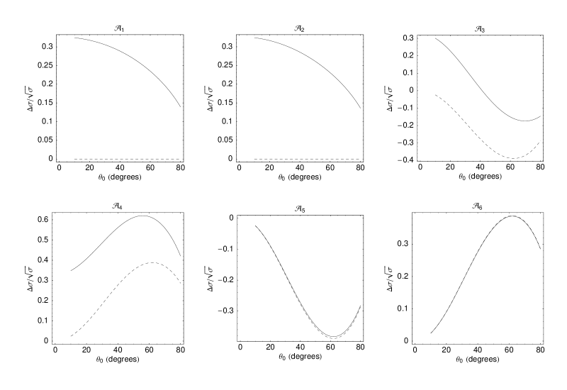
Figure 6: $\Delta\sigma/\sqrt{\sigma}$, which is proportional to the sensitivity $\mathcal{S}$, is plotted against the angular cut $\theta_{0}$ for all six asymmetries. Solid line is for the MSSM and dashed line for the SM. For $\mathcal{A}_{1}$ and $\mathcal{A}_{2}$, the smaller angular cut is favourable while for others $\theta_{0}=60^{\circ}$ is a good choice.

We define sensitivity as,

$${\cal S}=\frac{{\cal A}}{\delta{\cal A}}\propto\frac{\Delta\sigma}{\sqrt{\sigma}}.$$

$\Delta\sigma/\sqrt{\sigma}$, which is proportional to the sensitivity, is plotted for all asymmetries in Fig. 6 against the angular cut in the lab frame, $\theta_{0}$. Since $\mathcal{A}_{1}$ and $\mathcal{A}_{2}$ are purely CP-violating, they have no contribution from SM for any angular cut. Hence for them, the sensitivity is large when the angular cut is small, because of better statistics. For the other four there is an SM contribution that varies with the cut. Though the exact position of the peak in Fig. 6 depends upon the relative sizes and signs of the form factors, $\theta_{0}=60^{\circ}$ seems to be a good choice for the angular cut to maximise the sensitivity of four of the asymmetries.

The process under consideration violates CP in general. But when the cut $\theta_{0}$ is $0$, the partial cross sections for $l^{+}$ and $l^{-}$ production become the corresponding total cross sections, and are therefore equal, because of charge conservation. Hence for $\theta_{0}\rightarrow 0$, $\mathcal{A}_{5}$ and $\mathcal{A}_{6}$ approach zero. In that limit, the polarization asymmetries $\mathcal{A}_{3}$ and $\mathcal{A}_{4}$ are purely CP-violating. Thus for $\mathcal{A}_{3}$ and $\mathcal{A}_{4}$, apart from the choice $\theta_{0}=60^{\circ}$, where the sensitivity peaks, $\theta_{0}=0^{\circ}$ would also be a good choice for isolating CP-violating parameters. But, to be away from the beam pipe, we choose the lowest cut to be $20^{\circ}$ in the lab frame. We have used all six asymmetries for angular cuts of $20^{\circ}$ and $60^{\circ}$ to put limits on the combinations $x_{i}$ and $y_{i}$.

Figure 7: The boundaries of blind regions in the parameter space are plotted for various pairs of parameters, for luminosities 500 and 1000 fb^-1 at beam energy $E_{b}=$ 310 GeV. Both angular cuts, $\theta_{0}=20^{\circ}$ and $60^{\circ}$, are used to put limits at C.L. of 95%. The larger region corresponds to 500 fb^-1, while the smaller corresponds to 1000 fb^-1.

Table 1: List of 95% C.L. limits on all the combinations at 500 fb^-1 and 1000 fb^-1 at $E_{b}=$ 310 GeV. These limits are obtained from data plotted in Fig. 7.

	min	max	min	max	MSSM
	(500 fb-1)	(500 fb-1)	(1000 fb-1)	(1000 fb-1)	value
$x_{1}$	$-3.775$	3.594	$-2.990$	2.869	$-0.429$
$x_{2}$	$-3.413$	3.896	$-2.748$	3.111	$-0.396$
$x_{3}$	$-2.386$	2.873	$-1.842$	2.386	$-0.077$
$x_{4}$	$-2.837$	2.465	$-2.375$	1.930	$+0.165$
$y_{1}$	$-2.786$	2.786	$-2.148$	2.148	$-0.168$
$y_{2}$	$-3.095$	3.095	$-2.433$	2.433	$+0.363$
$y_{3}$	$-2.155$	2.155	$-1.687$	1.687	$-0.195$
$y_{4}$	$-2.346$	2.346	$-1.867$	1.867	$-0.180$

If for certain values of the form factors the asymmetries lie within the fluctuation from their SM values, then that particular point in the parameter space cannot be distinguished from SM at a given luminosity. That point will be said to fall in the blind region of the parameter space. Thus the set of parameters {$x_{i},y_{i}$} will be inside the blind region at a given luminosity if

$$|{\cal A}(\{x_{i},y_{i}\})-{\cal A}_{\rm SM}|\leq\delta{\cal A}_{\rm SM}=\frac{f}{\sqrt{\sigma_{\rm SM}{\cal L}}}\sqrt{1+{\cal A}_{\rm SM}^{2}}.$$ (56)

For simplicity we have taken only two of the eight combinations to be non-zero at a time and have constrained them in 16 different planes, shown in Fig. 7, satisfying their inter-relations. The limits obtained on each of the combinations by taking a union of the blind regions in the 16 plots are listed in Table 1. Also shown in the last column of the table are the values of $x_{i},y_{j}$ for the MSSM point we have chosen for Figs. 5 and 6.

Next we do a small exercise to see whether these asymmetries have the potential to distinguish between the SM and MSSM. It is clear that we can repeat the analysis of finding blind regions in the ($x_{i},y_{j}$) planes around a particular point predicted by the MSSM. The values of $x_{i},y_{j}$, corresponding to our choice of the MSSM point given by Eq. (49) are listed in last column of Table 1. The blind regions around these values will be defined by an equation similar to Eq. (56), where ${\cal A}_{\rm SM}$ will be replaced by ${\cal A}_{\rm MSSM}$. In ${\cal A}(x_{k},y_{l})$ all independent $x_{k},y_{l}$ other than the pair $x_{i},y_{j}$ being considered, are set to their MSSM value, and the pair $x_{i},y_{j}$ is then varied. We show in

Figure 8: The boundaries of blind regions in the parameter space are plotted in $x_{3}-y_{3}$ plane, for a luminosity of 1000 fb^-1 at beam energy $E_{b}=$ 310 GeV. Both angular cuts, $\theta_{0}=20^{\circ}$ and $60^{\circ}$, are used to put limits at C.L. of 95%. For this MSSM point, $x_{3}=-0.077,\ y_{3}=-0.195$.

Fig. 8 the results of such an exercise for the parameter pair ($x_{3},y_{3}$) along with the corresponding one for the SM. This shows that these studies can be sensitive to the CP mixing produced by loop effects. Of course one needs to study this over the supersymmetric parameter space. But the example shown here clearly shows the promise of the method.

VI Discussion

The four cross sections depending on the polarization of the initial lepton and the charge of the final state lepton that we use to construct asymmetries, can in general be written as

$$\sigma(\lambda_{e},Q_{l})=\sigma_{00}+\sigma_{01}Q_{l}+\sigma_{10}\lambda_{e}+\sigma_{11}Q_{l}\lambda_{e}.$$ (57)

This says that we have four independent $\sigma_{ij}$, which constitute four polarized cross-sections. Out of these four, $\sigma_{00}$ is the largest and others are of the order of a few per cent of $\sigma_{00}$. Thus we can safely approximate denominators of all ${\cal A}_{i}$’s to $\sigma=2\sigma_{00}$. This makes ${\cal A}_{i}$’s proportional to their numerators, which consists of only three of $\sigma_{ij}$. Thus out of six asymmetries constructed in Section V only three are independent and we cannot determine all six form factors simultaneously using these asymmetries. This is a reflection of the fact that there are only three CP-violating asymmetries wengan at the production level of the $t\bar{t}$ pair; one is for the unpolarized case, and the other two are polarization asymmetries. The ${\cal A}_{i}$’s defined here are combinations of these three.

In Fig. 7 we took only two combinations as non-zero and varied them to find the blind region in that plane. We found strong limits on $y$’s and almost no limits on $x$’s in each of the planes. When we allowed three of the combinations to vary simultaneously there were almost no limits on any of the combinations. This can be understood by looking at Eq. (57). The charge asymmetries are very small and approach zero as we reduce the angular cut, which implies that $\sigma_{01}$ and $\sigma_{11}$ are very small and tend to zero as $\theta_{0}\rightarrow 0$. Thus two of the four independent components of the polarized cross-section are very small (typically by a factor of 100 to 500); neglecting them, we are left with only two independent components, implying that only one of the six asymmetries is independent. Thus, though we have four independent components at hand, two being small we are effectively left with only two almost identical strong constraints, and thus essentially only one. These asymmetries thus constrain only $y$’s and leave $x$’s mostly unconstrained. The fact that $x$’s are constrained at all is because the equation of the boundary of a blind region arising from any one asymmetry, for two variables, is an equation of a pair of conic sections. The blind regions shown in Fig. 7 are intersections of blind regions obtained from all six asymmetries with two different angular cuts.

VI.1 The Strategy

All the cross sections and asymmetries are expressible in terms of $x$’s and $y$’s alone and, of these, only five are independent. Thus any number of asymmetries for any general polarization can never determine all six form factors as only five independent combinations appear in the expressions. For $S_{t}$ and $P_{t}$ we have to rely on partial decay width measurements of the scalar $\phi$ to $t\bar{t}$ pair. Thus, if we have a few more independent and strong constraints, we will be able to put simultaneous limits on all six form factors. But with circular polarization we have only the four observables used here already. One possibility would be to use the dependence of the angular distribution of the decay leptons on the initial state photon polarization. But to do that one would need a large statistics, which will not be available even with an integrated luminosity of $10^{3}$ fb^-1. The other option is to look for linearly polarized initial photons. Here, by choosing different angles between the planes of polarizations one can alter the relative contribution from CP-even and CP-odd Higgs. This, along with the asymmetries considered and the partial decay width of $\phi$, can then be used to put limits on all six form factors simultaneously or alternatively to determine them. Some discussions of these for the $t\bar{t}$ production exist already asakawa

In view of above analysis we can propose a strategy for characterizing the heavy scalar $\phi$. The first step would be to determine its mass $m_{\phi}$, its total decay width $\Gamma_{\phi}$ and the partial decay width to a $t\bar{t}$ pair. The last will tell us about $S_{t}^{2}+P_{t}^{2}$. Then the second step will be to look for asymmetries ${\cal A}_{1}$ and ${\cal A}_{2}$ to see if there is any CP violation. Step 3 depends upon the outcome of step 2. In case of non-observation of CP violation, one will have to look for linearly polarized asymmetries to see whether the Higgs is CP-even or CP-odd. If CP violation is observed, then all the asymmetries, for circular and linear polarizations, can be used to determine the form factors.

VI.2 Discriminating Models

As we have seen, it is not possible to determine all the combinations $x_{i},y_{j}$ using the asymmetries we have constructed. However, as discussed below, we can surely use the model predictions for these to discriminate against a particular model when data are available or test the possibilities of being able to distinguish between different models at a given luminosity.

The blind region around any model point in the five-dimensional parameter space is a non-convex structure and extends far out from the model point in some of the directions. Thus projection on any plane may result in a large blind region, which can be misleading. Thus it is not possible to restrict to less than the full set of 5 parameters for testing models. Below we develop a method for distinguishing between models and checking whether they are ruled out by experiment.

The simplest way to compare two models is to ask if the first model point lies within the blind region of the second and vice versa. If not, we say that the model predictions are distinguishable from each other at the luminosity and confidence level considered. As an example, we chose two models - SM and MSSM. The MSSM is same as given by the last column of Table 1.

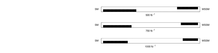
Figure 9: Blind regions along the line joining two model points, SM and MSSM, in the five-dimensional parameter space at ${\cal L}$ = 500, 750 and 1000 fb^-1. All six asymmetries with both angular cuts, $\theta_{0}=20^{0}$ and $60^{0}$, are used.

The model points in the five-dimensional parameter space are connected by a line parameterized by $t$ with $t=0$ corresponding to one model and $t=1$ to the other. We have calculated the blind region around each of the models along the connecting line. These are shown in Fig. 9 and it can be seen that each model sits well outside the blind region of the other at an integrated luminosity of 500 fb^-1. Furthermore, their blind regions do not overlap along these lines. Thus we can say that our method can distinguish candidate models at a certain luminosity (500 fb^-1 in this case). A more accurate way will be to search the whole of the five-dimensional parameter space for the overlap of the blind regions corresponding to two candidate models and not just along the line joining them. If no such overlap is found then we can say for sure that the models can be distinguished. This search could be quite complicated. Alternatively we can use the numerical values of individual asymmetries and fluctuations directly as discussed below.

It is clear that we can determine blind region around a given model prediction in any parameter space given the numerical value of the model predictions for asymmetries and the statistical fluctuations expected in it at a given luminosity. Any change in these numerical values will yield a different blind region in the five-dimensional parameter space. One will then test asymmetry predictions for a particular model against an experimental measurement or compare the predictions of two models against each other to draw conclusions about their distinguishability at a given luminosity and confidence level.

Table 2: The probability ${\cal P}$ of confusing SM with MSSM at 95% C.L. for different asymmetries and luminosities.

Asymmetries	${\cal P}$ at 500 fb-1	P at 750 fb-1	${\cal P}$ at 1000 fb-1
${\cal A}_{1}(\theta_{0}=60^{0})$	$5.5\times 10^{-4}$	$4.8\times 10^{-6}$	$6\times 10^{-8}$
${\cal A}_{2}(\theta_{0}=60^{0})$	$7.8\times 10^{-4}$	$8.0\times 10^{-6}$	$7\times 10^{-8}$
${\cal A}_{3}(\theta_{0}=60^{0})$	$3.4\times 10^{-4}$	$2.0\times 10^{-6}$	$1\times 10^{-8}$
${\cal A}_{4}(\theta_{0}=60^{0})$	$1.4\times 10^{-3}$	$2.1\times 10^{-6}$	$2.8\times 10^{-7}$
${\cal A}_{1}(\theta_{0}=20^{0})$	$1.6\times 10^{-7}$	$<10^{-8}$	$<10^{-8}$
${\cal A}_{2}(\theta_{0}=20^{0})$	$2.3\times 10^{-7}$	$<10^{-8}$	$<10^{-8}$
${\cal A}_{3}(\theta_{0}=20^{0})$	$2.3\times 10^{-7}$	$<10^{-8}$	$<10^{-8}$
${\cal A}_{4}(\theta_{0}=20^{0})$	$2.2\times 10^{-7}$	$<10^{-8}$	$<10^{-8}$

If the values of asymmetries expected at the particular level of confidence, corresponding to (say) two models, have no overlap, then the two models are distinguishable at that confidence level. There is still a non-zero probability that the models can be confused with each other in an experiment. To determine the probability of such a confusion we take any one asymmetry at a time and calculate the limits upto which the predicted asymmetry values can fluctuate at a certain level of confidence in the models under consideration. Then we generate normally distributed random numbers centered at the asymmetry corresponding to the first model, say SM, with standard deviation same as the 1 $\sigma$ fluctuation of the SM asymmetry. We count the number of points for which the asymmetry value lies within the 95% confidence interval of the other model, say MSSM. The number of such points divided by the total number of points taken is the probability ${\cal P}$ of confusing SM with MSSM at 95% confidence level. As Table 2 indicates, ${\cal P}$ is of the order of $10^{-7}$ for a luminosity of 500 fb^-1, and we can safely say that SM is distinguishable from MSSM at 500 fb^-1. In a similar way we can replace SM by the experimental asymmetries and MSSM by a candidate model. Now even if for one of the asymmetries ${\cal P}$ is very small ($O(10^{-3})$) we can simply reject the model as in words it translates to: the probability of the experimental results being statistical fluctuation of the candidate model at 95% C.L. is very small. In fact, the method described above is nothing but the Step 2 of our strategy discussed in previous sections, when one talks about asymmetries ${\cal A}_{1}$ and ${\cal A}_{2}$.

VII Conclusion

We have demonstrated how the Higgs-mediated CP violation in the process $\gamma\gamma\rightarrow t\bar{t}$ can be studied by looking at the integrated cross section of $l^{+}/l^{-}$ coming from the decay of $t/\bar{t}$. We demonstrated that the decay lepton angular distribution is insensitive to any anomalous part of the $tbW$ coupling, $f^{\pm}$, to first order. We constructed combined asymmetries involving the initial lepton (and hence the photon) polarization and the decay lepton charge. We showed that using only circularly polarized photons will be inadequate to determine or constrain the sizes of all form factors simultaneously, but can put strong limits on CP-violating combinations, $y$’s, when only two combinations are varied at a time. We show, by taking an example of a particular choice of MSSM parameters, that the analysis is sensitive to the CP mixing at a level that is generated by loop effects. We also further sketch a possible strategy to characterize the scalar $\phi$ using linear polarization.

ACKNOWLEDGEMENT

We thank Prof. N. V. Joshi for useful discussions.

Appendix A Expressions for $A_{ij}$, $B_{ij}$, etc.

For circularly polarized photons the form factors $A_{ij}$ and $B_{ij}$ are given below; $\eta_{2}$ and $\xi_{2}$ are the degrees of circular polarization of two colliding photons:

$$A_{00}^{\pm} = 2|A_{\phi}|^{2}(\beta^{2}S_{t}^{2}+P_{t}^{2})\left[(|S_{\gamma}|^{2}+|P_{\gamma}|^{2})\right.$$

$$\left.\left(\frac{1+\eta_{2}\xi_{2}}{2}\right)+2\Im(S_{\gamma}P^{*}_{\gamma})\left(\frac{\eta_{2}+\xi_{2}}{2}\right)\right]$$

$$A_{01}^{\pm} = 4A_{c}\left[(\beta^{2}S_{t}\Re(A_{\phi}S_{\gamma})+P_{t}\Re(A_{\phi}P_{\gamma}))\left(\frac{1+\eta_{2}\xi_{2}}{2}\right)\right.$$

$$+ \left.(P_{t}\Im(A_{\phi}S_{\gamma})-\beta^{2}S_{t}\Im(A_{\phi}P_{\gamma}))\left(\frac{\eta_{2}+\xi_{2}}{2}\right)\right]$$

$$A_{02}^{\pm} = 2A_{c}^{2}\left[(1+\beta^{2})\left(\frac{1+\eta_{2}\xi_{2}}{2}\right)\right.$$

$$+ \left.\frac{\beta^{2}(2-\beta^{2})}{1-\beta^{2}}\left(\frac{1-\eta_{2}\xi_{2}}{2}\right)\right]$$

$$A_{22}^{\pm} = -4A_{c}^{2}\beta^{2}\left(\frac{1-\eta_{2}\xi_{2}}{2}\right)$$

$$A_{42}^{\pm} = -\frac{2A_{c}^{2}\beta^{4}}{1-\beta^{2}}\left(\frac{1-\eta_{2}\xi_{2}}{2}\right)$$

$$B_{01}^{\pm} = 4\beta A_{c}\left[(S_{t}\Re(A_{\phi}S_{\gamma})+P_{t}\Re(A_{\phi}P_{\gamma}))\left(\frac{\eta_{2}+\xi_{2}}{2}\right)\right.$$

$$+ \left.(P_{t}\Im(A_{\phi}S_{\gamma})-S_{t}\Im(A_{\phi}P_{\gamma}))\left(\frac{1+\eta_{2}\xi_{2}}{2}\right)\right]$$

$$B_{02}^{\pm} = 4\beta A_{c}^{2}\left(\frac{\eta_{2}+\xi_{2}}{2}\right)$$

$$B_{12}^{\pm} = \frac{4A_{c}^{2}\beta^{2}}{1-\beta^{2}}\left(\frac{\eta_{2}-\xi_{2}}{2}\right)=\ B_{12}$$

$$B_{32}^{\pm} = -B_{12}^{\pm}=-B_{12}$$

$$C_{0} = 4\beta^{2}A_{c}^{2}\left(\frac{\eta_{2}-\xi_{2}}{2}\right)$$

$$D^{\pm} = 0$$

$$A_{c} = \frac{4Q_{t}^{2}m_{t}}{\sqrt{s}}=2Q_{t}^{2}\sqrt{1-\beta^{2}}$$

$$A_{\phi} = \frac{e}{16\pi^{2}}\ \frac{m_{t}}{m_{W}}\ \frac{s}{s-m_{\phi}^{2}+im_{\phi}\Gamma_{\phi}}$$

$$X_{0} = 2+\beta^{2}\sin^{2}\theta_{l}$$

$$X_{1} = -4\beta\cos\theta_{l}$$

$$X_{2} = \beta^{2}(3\cos^{2}\theta_{l}-1)$$

$$Y_{0} = -\cos\theta_{l}(2+\beta^{2}\sin^{2}\theta_{l})$$

$$Y_{1} = \beta(3+\cos^{2}\theta_{l})$$

$$Y_{2} = 2\cos\theta_{l}(2-\beta^{2}\cos^{2}\theta_{l})$$

$$Y_{3} = -2\beta(3+\cos^{2}\theta_{l})$$

$$Y_{4} = \cos\theta_{l}(-2+3\beta^{2}+\beta^{2}\cos^{2}\theta_{l})$$

$$Y_{5} = \beta(3+\cos^{2}\theta_{l})$$

$$Y_{6} = -2\beta^{2}\cos\theta_{l}$$

References

- (1) J. A. Aguilar-Saavedra et al. [ECFA/DESY LC Physics Working Group Collaboration], hep-ph/0106315; B. Badelek et al. [ECFA/DESY Photon Collider Working Group Collaboration], hep-ex/0108012.
- (2) S. Weinberg, Phys. Rev. Lett. 37 (1976) 657.
- (3) T. D. Lee, Phys. Rep. C 9 (1974) 143.
- (4) A. Pilaftsis and C. E. M. Wagner, Nucl. Phys. B553 (1999) 3 (hep-ph/9902371); S. Y. Choi, M. Drees and J. S. Lee, Phys. Lett. B481 (2000) 57; M. Carena, J. Ellis, A. Pilaftsis and C. E. M Wagner, Nucl. Phys. B586 (2000) 92 (hep-ph/0003180), S.Y. Choi and J.S. Lee, Phys. Rev. D62 (2000) 036005 (hep-ph/9912330).
- (5) E. Asakawa, J.-i. Kamoshita, A. Sugamoto and I. Watanabe, Eur. Phys. J. C 14 (2000) 335 (hep-ph/9912373).
- (6) S. Bae, B. Chung and P. Ko, hep-ph/0205212; S.Y. Choi, B. Chung, P. Ko and J.S. Lee, hep-ph/0206025.
- (7) E. Asakawa, S. Y. Choi, K. Hagiwara and J. S. Lee, Phys. Rev. D62 (2000) 115005 (hep-ph/0005313).
- (8) B. Grzadkowski and J. F. Gunion, Phys. Lett. B 294 (1992) 361–368.
- (9) G. Jikia and S. Soldner-Rembold, in Ref. 1; Nucl. Instrum. Meth. A 472 (2001) 133 (hep-ex/0101056).
- (10) P. Niezurawski, A.F. Zarnecki and M. Krawczyk, hep-ph/0207294.
- (11) S. Y. Choi, D. J. Miller, M. M. Muhlleitner and P. M. Zerwas, hep-ph/0210077.
- (12) M. M. Muhlleitner, M. Kramer, M. Spira and P. M. Zerwas, Phys. Lett. B 508 (2001) 311 (hep-ph/0101083).
- (13) I. F. Ginzburg, G. L. Kotkin, S. L. Panfil, V. G. Serbo and V. I. Telnov, Nucl. Instrum. Meth. 294 (1984) 5.
- (14) A.F. Zarnecki, CompAZ: parametrization of the photon collider luminosity spectra, submitted to ICHEP’ 2002, abstract #156; hep-ex/0207021. http://info.fuw.edu.pl/∼zarnecki/compaz/compaz.html
- (15) V. I. Telnov, Nucl. Instrum. Meth. A 355 (1995) 3; A code for the simulation of luminosities and QED backgrounds at photon colliders, talk presented at Second Workshop of ECFA-DESY study, Saint-Malo, France, April 2002.
- (16) R.M. Godbole, S.D. Rindani and R.K. Singh, In preparation.
- (17) G. Jikia and A. Tkabladze, Phys. Rev. D 54 (1996) 2030 (hep-ph/9601384); Phys. Rev. D 63 (2001) 074502 (hep-ph/0004068).
- (18) M. Melles, W. J. Stirling and V. A. Khoze, Phys. Rev. D 61 (2000) 054015 (hep-ph/9907238).
- (19) S.D. Rindani, Pramana 54 (2000) 791 (hep-ph/0002006).
- (20) B. Grzadkowski and Z. Hioki, Phys. Lett. B 476 (2000) 87 (hep-ph/9911505); Z. Hioki, hep-ph/0104105.
- (21) K. Ohkuma, Nucl.Phys.Proc.Suppl. 111 (2002) 285, (hep-ph/0202126).
- (22) B. Grzadkowski and Z. Hioki, Phys. Lett. B 529 (2002) 82, (hep-ph/0112361).
- (23) B. Grzadkowski and Z. Hioki, FT-19-02, (hep-ph/0208079); Z. Hioki, hep-ph/0210224.
- (24) S.Y. Tsai, Phys. Rev. D 4 (1971) 2821; S. Kawasaki, T. Shirafuji and S.Y. Tsai, Prog. Theo. Phys. 49 (1973) 1656.
- (25) P. Poulose and S.D. Rindani, Phys. Rev. D 57 (1998) 5444, D 61 (2000) 119902 (E); Phys. Lett. B 452 (1999) 347; P. Poulose, Nucl. Instrum. Meth. A 472 (2001) 195.
- (26) W.-G. Ma, C.-H Chang, X.-Q. Li, Z.-H. Yu and L. Han, Commun. Theor. Phys. 26 (1996) 455; Commun. Theor. Phys. 27 (1997) 101.