AN ELECTROWEAK WEIZSÄCKER-WILLIAMS METHOD

Abstract

© Copyright by Sean Ahern, 2001
All Rights Reserved

AN ELECTROWEAK WEIZSÄCKER-WILLIAMS METHOD

Dedication

To

my parents, my sister

and

my fiancée

Chapter 1 Introduction

The physics of interacting charged particles can be quite complicated. The situation simplifies considerably if the particles are travelling at very nearly the speed of light. Due to relativistic effects, the electric $\boldsymbol{E}$ and magnetic $\boldsymbol{B}$ fields of such a particle are (Lorentz) contracted into the plane that is transverse to the direction of motion. At every point in this plane, the $\boldsymbol{E}$ and $\boldsymbol{B}$ fields are of very nearly the same magnitude and are transverse to one another, very much like on the wavefront of a plane electromagnetic (EM) wave. In fact, to an observer (viz, another particle) at rest some short distance away from the passing particle, the effects of these fields are practically indistinguishable from those of a passing EM wave. If the particle’s EM fields are approximated as EM plane waves, the problem of analyzing a peripheral (near-miss) collision of two ultrarelativistic (UR) charged particles thus simplifies to one of analyzing the interaction between a passing EM wave and just one particle.

This idea was first introduced in 1924 by E. Fermi, and extended ten years later by C. Weizsäcker and E. Williams, and forms the basis of what is now called the Weizsäcker-Williams method (WWM), or Equivalent Photon Approximation (EPA) [1, 2]. Since then, much progress has been made, including the development of a quantum mechanical version of the method (QWWM) that is in very good agreement (in the UR limit) with the original semiclassical version (SWWM) [2, 3, 4]. The most basic approximations of both variants of the WWM are that (1) the colliding particles are ultrarelativistic; (2) the particles follow straight-line trajectories; and (3) the particles have no internal structure. Various complications have been introduced throughout the years, including the relaxation of approximations (2) and (3), but in its simplest form, the WWM turns out to be an impressively accurate approximation scheme. A brief informative survey of the history of the WWM is presented in [5]. The success of the Standard Model (SM) (viz, the electroweak sector) has brought about the development of a weak interaction analog of the QWWM, called the Effective-$W$ Method (EWM) [6, 7, 8, 9, 10, 11]. The only difference between the EWM and the QWWM is that the particles mediating the interactions are $W$ and $Z$ bosons instead of photons. Like the QWWM, the EWM is a very accurate alternative to the more exact theory.

The purpose of this thesis is to generalize the scope of the SWWM so as to accommodate $W$ and $Z$ bosons, in addition to photons, as the mediators of the particle collisions. The motivation for this endeavor is threefold. First, the SM is generally believed to only be a low energy approximation to a more (as yet undiscovered) comprehensive theory; it is only reliable up to interaction energies of about the TeV scale. For energies above about a TeV, a different approach (one not based on perturbation theory) is needed. Currently, the EWM is the only such viable alternative [8]. However, the EWM assumes that the mediating bosons are on-shell (“real”), so in principle it cannot be used to investigate interactions in which the bosons are necessary off-shell (“virtual”). An example of such an interaction is the production of a sufficiently light-weight resonance $R$ via $W$ or $Z$ boson fusion in fermion-fermion scattering (cf. Fig. 1). The EWM can be used if the two bosons are real and the mass of $R$ is greater than the sum of their masses. However, if the mass of $R$ is less than the sum of the on-shell values of the boson masses, conservation of energy precludes the reaction from proceeding unless the bosons are virtual. But, in that case, the EWM is not applicable because it assumes that the bosons are real. So, the second goal of this research is to formulate a scheme in which the mediating bosons are not necessarily on-shell, with the hope that it might have a greater scope of applicability than the EWM. The last factor is pedagogical — such a generalization has never been done before. With the phenomenal success of the electroweak theory within the past few decades, it seems timely to return to the classical theory to try to formulate a classical (or, at least semiclassical) description of the same phenomena. Perhaps interesting parallels can be drawn between the two viewpoints.

There are usually two parts to the typical SWWM analysis — a semiclassical part and a quantum part. For concreteness in understanding the implementation of the method, consider the prototypical interaction shown in Fig. 2. An incident particle $q$ undergoes a peripheral collision with a target particle $P$ by way of a one-photon exchange. The semiclassical part of the calculation is concerned with the emission of EM energy $\gamma$ (a photon in the quantum viewpoint) from $q$. The useful quantity is the number spectrum $N(E)$ of photons — the differential number d$n(E)$ of photons of energy $E$ in $q$’s EM fields per unit photon energy d$E$:

$$N(E)=\frac{\mathrm{d}n(E)}{\mathrm{d}E}\qquad\mbox{(number spectrum).}$$ (1)

Usually, the quantum part involves the description of the interaction between the emitted photon and a target particle ($P$ in this case). The quantity of interest here is the (microscopic) cross section $\sigma_{mic}$ for this photon-induced subprocess. The (macroscopic) cross section $\sigma_{mac}$ for the overall process is found by folding $N(E)$ with $\sigma_{mic}$:

$$\sigma_{mac}=\int\mathrm{d}E\,N(E)\,\sigma_{mic},$$ (2)

where the integral runs over all allowable (by energy conservation) photon energies. So, in a crude sense, $N(E)$ gives the probability that $q$ emits the photon $\gamma$ at energy $E$, and $\sigma_{mic}$ is the probability that $\gamma$ then collides with $P$ and produces the final state $X$. A more interesting application of the method is where two bosons are simultaneously exchanged, and collide to produce some final state $X$. The microscopic cross section then describes the two-boson-induced subprocess. An example of one such process is SM Higgs boson production via boson-boson fusion (cf. Fig. 3). The Higgs boson is the last remaining unverified prediction of the SM that presumably endows all particles with mass. For more information on this interesting particle, see [12], [13], or practically any other reference on modern particle physics. For such a two-boson process, $\sigma_{mac}$ is of the form

$$\sigma_{mac}=\int\mathrm{d}E_{1}\int\mathrm{d}E_{2}\;\,N(E_{1})\,N(E_{2})\,\sigma_{mic}.$$ (3)

The expression for the macroscopic cross section in the SWWM, QWWM and EWM all share this same form, but whereas $N(E)$ is calculated using semiclassical considerations in the SWWM, it is treated quantum mechanically in both the QWWM and EWM. The determination of $\sigma_{mic}$ is a quantum calculation in all of these schemes. The method developed here is formulated in much the same spirit as in the (traditional) SWWM — the $N(E)$ functions are derived semiclassically and $\sigma_{mic}$ is derived using quantum field theory. So, like the SWWM, this scheme is semiclassical in nature.

This document is arranged as follows. Chapter 2 summarizes the notation and conventions that will be used, and the overall scenario that is under consideration. In Chapter 3, the number spectrum function $N(E)$ is derived in a more general way than is done in the traditional analysis — allowing for bosons with some (as yet unspecified) nonzero mass. In Chapter 4, $N(E)$ is shown to reduce to the relevant functions (that appear in the other above-mentioned methods) in the various limits of interest when a few extra reasonable assumptions are made. And, finally, in Chapter 5, the results obtained using the current approach are compared to those of other studies.

Chapter 2 Notation, Conventions and Overall Scenario

Natural units (rationalized Heaviside-Lorentz units (where $\varepsilon_{0}=\mu_{0}=1$) with $\hbar=c=1$) and the Einstein summation convention (the repeated appearance of the same index in any tensor equation implies a sum over all allowable values) are used throughout. Greek indices $\mu,\,\nu,\,\xi,\,\ldots$ can take on the values $0,\,1,\,2,\,3,\mbox{ or }4$, and Latin indices $i,\,j,\,k,\,\ldots$ can only take on the values $1,\,2\mbox{ or }3$. The signature of the metric is taken to be $+\,-\,-\,-$ , so that

$$g^{\mu\nu}=g^{\nu\mu}=\begin{pmatrix}1&\;\;\;0&\;\;\;0&\;\;\;0\\ 0&-1&\;\;\;0&\;\;\;0\\ 0&\;\;\;0&-1&\;\;\;0\\ 0&\;\;\;0&\;\;\;0&-1\end{pmatrix}\qquad\mbox{(metric tensor).}$$ (1)

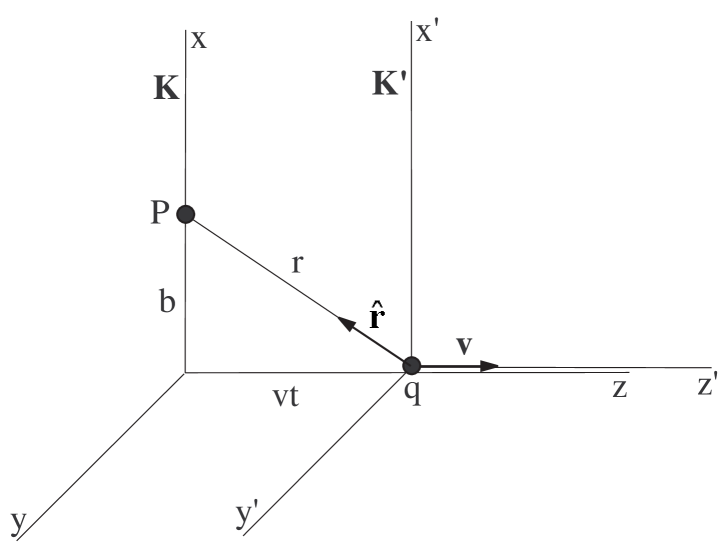
FIG. 4: A particle $q$ at rest at the origin of frame $K^{\prime}$ moves in the $z/z^{\prime}$ direction past point $P$ in frame $K$ with velocity $\boldsymbol{v}$. Relative to the origin of $K$, $P$ is located at coordinates $(b,\,0,\,0)$ and the coordinates of $q$ are $(0,\,0,\,vt)$.

Of interest is a peripheral collision between an incident particle $q$ and some target point $P$. $P$ can be thought of as another particle or merely an interaction point; a prototypical Feynman diagram that takes $P$ to be an actual particle appears in Fig. 2. At the point of closest approach between $q$ and $P$, a boson (either a photon or a $W$ or $Z$ boson) is emitted by $q$ that subsequently interacts with some other particle at $P$. It is convenient to proceed from the standpoint of an observer at rest in the frame comoving with $P$, who views $q$ pass by with some UR speed $v\simeq 1$. The basic scenario is depicted in Fig. 4. Frames $K$ (rest frame of $P$) and $K^{\prime}$ (rest frame of $q$) share a common $z$ axis and coincide at time $t=t^{\prime}=0$. $q$ is located at the origin of $K^{\prime}$ and moves at constant velocity $\boldsymbol{v}=\boldsymbol{\hat{v}}v$ (with magnitude $v$ and direction $\boldsymbol{\hat{v}}$) past $P$ along the common $z/z^{\prime}$ axis (the identifications $\boldsymbol{\hat{v}}=\boldsymbol{\hat{z}}$ in $K$ and $\boldsymbol{\hat{v}}=\boldsymbol{\hat{z}^{\prime}}$ in $K^{\prime}$ can always be made). $P$ is located at a fixed perpendicular distance $b$ (the “impact parameter”) from the $z/z^{\prime}$ axis, along the $x$ axis. $b$ is also the distance of closest approach between $q$ and $P$, which occurs at time $t=t^{\prime}=0$.

As the WWM formalism is (by construction) only valid at high energies, the most frequent approximation made throughout this thesis is that the colliding particles (both fermions and bosons) are travelling at UR speeds. This condition is alternatively expressed as $v=|\boldsymbol{p}|/E\simeq 1$, $\gamma=E/m\gg 1$, etc., where

$$\gamma=\frac{1}{\sqrt{1-v^{2}}}\qquad\mbox{(Lorentz factor)}$$ (2)

is the Lorentz factor. It will be assumed that any errors introduced by this approximation are negligible.

Lastly, the symbols $\gamma$, $Z$ and $W$ are used to label quantities corresponding to EM, neutral weak and charged weak interactions, respectively. It should be clear from the context whether $\gamma$ means $1/\sqrt{1-v^{2}}$ or is a label identifying an EM quantity, and whether $Z$ means $z$ axis or $Z$ boson, and so on.

Chapter 3 Derivation of $N(E)$

The derivation of $N(E)$ consists of two separate analyses. One is the specification of the scalar $\Phi$ and vector $\boldsymbol{A}$ potentials and the $\boldsymbol{E}$ and $\boldsymbol{B}$ fields of an UR charged particle $q$. The other is the determination of the same set of quantities for relevant plane waves of radiation in a vacuum. The next step, which is the hallmark of the WWM, is to make appropriate identifications between the two sets of quantities, and thereby approximate the fields of $q$ as equivalent pulses of plane wave radiation. This approximation is known to work in the SWWM, and will be shown to be interconsistent as well in the generalized version (GWWM) developed herein. The identification allows for the interpretation of the fields as quantum mechanical bosons, and hence makes plausible the subsequent quantum field theoretic treatment of any boson-induced microscopic cross section of interest.

As mentioned briefly in the Introduction, the function $N(E)$ is the differential number of bosons of energy $E$ in the fields surrounding $q$ per unit boson energy. The quantity of paramount importance in the derivation of $N(E)$ is the Poynting vector $\boldsymbol{S}(\boldsymbol{r},t)$, or energy flux, associated with the fields of $q$. With appropriate factors of $\hbar$ taken into account, $N(E)$ can be thought of as the Fourier transform (FT) $\boldsymbol{S}(\boldsymbol{r},\omega)$ of $\boldsymbol{S}(\boldsymbol{r},t)$, integrated over the (infinite) wavefront area of the equivalent pulse, and divided by the energy $E=\omega$ of the bosons. The analysis thus begins with a general (coordinate-independent) discussion of the Poynting vector $\boldsymbol{S}$.

3.1 Energy Flux

Insofar as energy transport by radiation is concerned, the most descriptive dynamic quantity is the Poynting vector $\boldsymbol{S}$, which represents the energy flux (energy per unit time per unit area) carried by the wave. It is a familiar result from classical electrodynamics (ED) that $\boldsymbol{S}=\boldsymbol{E}\times\boldsymbol{B}$ in a source-free region. This short section sets the stage for future calculations by stating the generalization of this formula to cases where the fields have some nonzero mass $m$.

The $i^{th}$ component of $\boldsymbol{S}$ is the $i0^{th}$ component of the stress-energy tensor $T^{\mu\nu}$: $S^{i}=T^{i0}$. More generally, $T^{\mu\nu}=T^{\nu\mu}$ is the flow of the $\mu^{th}$ component of 4-momentum along the $\nu$ direction. The generalization being sought can be derived using standard variational techniques once the Lagrangian is known. For a massive spin-1 field, the result is (see [14], for example)

$$\boldsymbol{S}=\boldsymbol{E}\times\boldsymbol{B}+m^{2}\Phi\boldsymbol{A}-\rho\boldsymbol{A},$$ (1)

where $\Phi$, $\boldsymbol{A}$, $\boldsymbol{E}$, $\boldsymbol{B}$ are the aforementioned scalar and vector potentials, and electric and magnetic fields, respectively, and $\rho$ is the charge density of the source. In the case under consideration, the region of space at the observation point, where $\boldsymbol{S}$ is to be evaluated, is source-free. So $\rho=0$ and Eq. (1) becomes

$$\boldsymbol{S}=\boldsymbol{E}\times\boldsymbol{B}+m^{2}\Phi\boldsymbol{A}.$$ (2)

Note that Eq. (2) consistently reduces to the familiar expression $\boldsymbol{S}=\boldsymbol{E}\times\boldsymbol{B}$ in the $m=0$ limit. It’s also important to note that in the $m=0$ limit, the functional forms of $\Phi$ and $\boldsymbol{A}$ are inconsequential insofar as the physically measurable $\boldsymbol{S}$ is concerned. This subtlety has its roots in gauge field theory. It is a familiar result from classical ED that the solutions to Maxwell’s equations (ME) are arbitrary up to a choice of gauge. More specifically, there is a whole family of functions $\Phi$ and $\boldsymbol{A}$ that yield the same $\boldsymbol{E}$ and $\boldsymbol{B}$ fields, which are the only quantities of any importance in determining $\boldsymbol{S}$. The same cannot be said for the massive field case — if $m\neq 0$, there is no arbitrariness allowed to any of these functions.

3.2 Potentials and Fields of an UR Point Charge

The potentials and fields of $q$ are first solved for in $K^{\prime}$, the rest frame of $q$, and are then (Lorentz) transformed to frame $K$, the rest frame of $P$, where they are evaluated at the location of $P$.

3.2.1 $\Phi^{\prime}(\boldsymbol{r^{\prime}},t^{\prime})$ and $\boldsymbol{A^{\prime}}(\boldsymbol{r^{\prime}},t^{\prime})$ of a Point Charge at Rest

The equations of motion for the four vector bosons (the radiation fields in the semiclassical picture) appearing in the SM are generally quite complex. The equations of motion for a given field have vestiges of the other three bosons. These “coupling terms” arise mathematically because the SU(2) algebra describing the interactions is nonabelian (noncommutative). More intuitively, the terms correspond to interactions among the bosons. In particular, interactions couple $W^{+}$ and $W^{-}$ bosons to each other and to $Z$ bosons and photons. Photons and $Z$ bosons do not interact because photons only couple to electrically charged particles, and $Z$ bosons are electrically neutral. For the problem of interest to this thesis, the coupling terms naturally disappear from the equations because the interactions of interest only involve bosons being emitted from fermions. In the language of quantum field theory, the processes are always tree-level fermion-boson interactions, so there are no further boson-boson couplings to consider. For a given boson, one simply sets all other boson fields to zero. A detailed presentation of this procedure, applied to decoupling the $Z$ boson and photon equations of motion, is given in [15]. The following analysis implicitly assumes that such a step has already been carried out, so that the field equations for the four bosons are uncoupled from one another.

The functions $\Phi$ and $\boldsymbol{A}$, describing the radiation fields, are combined into a 4-vector called the 4-potential,

$$A^{\mu}=(\Phi,\boldsymbol{A})\qquad\mbox{(4-potential),}$$ (3)

and the charge $\rho$ and current $\boldsymbol{J}$ densities, describing the source charge, are combined into the 4-current:

$$J^{\mu}=(\rho,\boldsymbol{J})\qquad\mbox{(4-current).}$$ (4)

For massless fields (photons), the equations of motion linking $A^{\mu}$ and $J^{\mu}$ are ME:

$$\Box A^{\mu}=J^{\mu}\qquad\mbox{(Maxwell's equations).}$$ (5)

For massive fields ($W$ and $Z$ bosons), the set of equations is called the Proca equation (PE):

$$\Box A^{\mu}+m^{2}A^{\mu}=J^{\mu}\qquad\mbox{(Proca equation).}$$ (6)

Both sets of field equations are shown here after the Lorentz condition (LC), $\partial^{\mu}A_{\mu}=0$, has already been imposed. The LC is an optional constraint in the former case, but is a natural consequence of current conservation in the latter. $\Box$ is the D’Alembertian operator,

$$\Box=\partial^{\mu}\partial_{\mu}=\frac{\partial^{2}}{\partial t^{2}}-\boldsymbol{\triangledown}^{2}\qquad\mbox{(D'Alembertian operator),}$$ (7)

and the quantity $m$ appearing in Eq. (6) is the mass of the boson, which, for the usual application to on-shell $W$ and $Z$ bosons, is set equal to $80.42$ and $91.19$ GeV, respectively [16]. For the sake of generality, the analysis will be confined entirely to the PE (note that ME are the $m=0$ limit of the PE), and $m$ will be left unspecified for the time being. Later, special cases of interest, where the appropriate value of $m$ will be explicitly stated, will be considered. From time to time, $m$ will be set to $0$ in the formulas to verify that they correctly reduce to those of the SWWM.

The starting point is thus Eq. (6). This equation will first be solved for a point charge $q$ at rest (in frame $K^{\prime}$). ${A^{\mu}}^{\prime}$ does not explicitly depend on time, as the source is simply a static charge at rest, so $\partial{A^{\mu}}^{\prime}/\partial t^{\prime}=0$, and Eq. (6) reduces to

$$\boldsymbol{\triangledown}^{2}{A^{\mu}}^{\prime}-m^{2}{A^{\mu}}^{\prime}=-{J^{\mu}}^{\prime}.$$ (8)

The solution is a standard exercise in Fourier analysis (see [17], or the methods outlined in [1], for example). In frame $K^{\prime}$, ${A^{\mu}}^{\prime}$ is found to be

$${A^{\mu}}^{\prime}(\boldsymbol{r^{\prime}},t^{\prime})=\frac{1}{4\mathrm{\pi}}\,\int\mathrm{d}^{3}\boldsymbol{\bar{r}^{\prime}}\,\frac{{J^{\mu}}^{\prime}(\boldsymbol{\bar{r}^{\prime}},t^{\prime})}{|\boldsymbol{r^{\prime}}-\boldsymbol{\bar{r}^{\prime}}|}\,\mbox{\Large e}^{-m|\boldsymbol{r^{\prime}}-\boldsymbol{\bar{r}^{\prime}}|},$$ (9)

where $\boldsymbol{r^{\prime}}=\boldsymbol{r^{\prime}}(t^{\prime})$ and $\boldsymbol{\bar{r}^{\prime}}=\boldsymbol{\bar{r}^{\prime}}(t^{\prime})$ are the position vectors of $P$ and $\mathrm{d}q$ (the differential source charge element within $q$), respectively. From basic Lorentz transformation (LT) equations, it is known that the position vector of $P$ in $K^{\prime}$ is $\boldsymbol{r^{\prime}}(t^{\prime})=(b,\,0,\,-vt^{\prime})$, and it might be expected that $\boldsymbol{\bar{r}^{\prime}}(t^{\prime})=(0,\,0,\,0)$, as $q$ is supposed to be a point charge located at the origin of $K^{\prime}$.

After a moderate amount of work, a form for $J^{\mu}(\boldsymbol{r},t)$ that is common to all three types of electroweak (EW) interactions of point charges can be found. The derivation is presented in Appendix A. The result is

$$J^{\mu}(\boldsymbol{r},t)=\delta[\boldsymbol{r}(t)]\,q^{\mu}\qquad\mbox{(4-current of a point charge).}$$ (10)

$\delta[\boldsymbol{r}(t)]$ is the (3 dimensional) Dirac delta function, that forces all $\mathrm{d}q$ elements to be located at the same point, $\boldsymbol{r}(t)=\boldsymbol{0}$. $q^{\mu}=(q^{0},\boldsymbol{q})$ is a new 4-vector introduced here, called the “4-charge”. It can be expressed in all cases of interest as a linear combination of the 4-velocity $u^{\mu}$ and normalized 4-spin $s^{\mu}$ of the particle:

$$q^{\mu}=q_{V}u^{\mu}+q_{A}s^{\mu}\qquad\mbox{(4-charge).}$$ (11)

The subscripts $V$ and $A$ on the coefficients $q_{V}$ and $q_{A}$ refer to the fact that $u^{\mu}$ and $s^{\mu}$ are vector and axial-vector quantities, respectively. $u^{\mu}$ can always be written as

$$u^{\mu}=\gamma(1,\boldsymbol{\hat{v}}v)\qquad\mbox{(4-velocity),}$$ (12)

and $s^{\mu}$ is expressed in a simple way in terms of the helicity $\lambda$ of the particle, as

$$s^{\mu}=\gamma(\lambda v,\boldsymbol{\hat{s}})\qquad\mbox{(normalized 4-spin).}$$ (13)

$\boldsymbol{\hat{s}}$ is the normalized spin (3-vector) of the particle, which is chosen to be measured along the $z$ axis so that $\boldsymbol{\hat{s}}=+\boldsymbol{\hat{z}}$ for spin-up and $\boldsymbol{\hat{s}}=-\boldsymbol{\hat{z}}$ for spin-down. Helicity is the normalized projection of the particle’s spin along the direction of motion, and can be expressed in terms of $\boldsymbol{\hat{s}}$ as

$$\lambda=\boldsymbol{\hat{s}}\cdot\boldsymbol{\hat{v}}\qquad\mbox{(helicity).}$$ (14)

See Appendix B for a more in depth discussion of helicity. Because $\boldsymbol{v}$ is being chosen to be along the $z$ axis, $\boldsymbol{\hat{s}}$ can also be written as

$$\boldsymbol{\hat{s}}=\boldsymbol{\hat{z}}\lambda\qquad\mbox{(normalized 3-spin),}$$ (15)

where $\lambda=\boldsymbol{\hat{s}}\cdot\boldsymbol{\hat{z}}=+1(-1)$ for spin-up(down). While the helicity of a massive particle is not Lorentz invariant in general, it can be easily shown that for the simple Lorentz boost that will be considered here (where $\boldsymbol{\hat{v}}$ is fixed in direction), $\lambda^{\prime}=\lambda$ is constant. Plugging Eq. (15) into Eq. (13), and using $\boldsymbol{\hat{v}}=\boldsymbol{\hat{z}}$, the general result

$$s^{\mu}=\gamma\lambda(v,\boldsymbol{\hat{z}})$$ (16)

is found. $q^{\mu}$ can then be written

$$q^{\mu}=\gamma((q_{V}+q_{A}\lambda v),\boldsymbol{\hat{z}}(q_{V}v+q_{A}\lambda)).$$ (17)

For completeness, $u^{\mu}$, $s^{\mu}$, $q^{\mu}$, and $J^{\mu}$ are now specified in two limiting cases of interest: the zero-velocity limit (i.e., the rest frame $K^{\prime}$ of the charge $q$ itself, where $v=0$), and the UR limit (i.e., the rest frame $K$ of the observer $P$, where $v=1$). In the former limit (with $\boldsymbol{\hat{z}}=\boldsymbol{\hat{z}^{\prime}}$),

$${u^{\mu}}^{\prime}=(1,\boldsymbol{0})\qquad\mbox{(rest frame),}$$ (18)

$${s^{\mu}}^{\prime}=(0,\boldsymbol{\hat{z}^{\prime}}\lambda)\qquad\mbox{(rest frame),}$$ (19)

$${q^{\mu}}^{\prime}=(q_{V},\boldsymbol{\hat{z}^{\prime}}q_{A}\lambda)\qquad\mbox{(rest frame),}$$ (20)

and

$${J^{\mu}}^{\prime}(\boldsymbol{r^{\prime}},t^{\prime})=\delta[\boldsymbol{r^{\prime}}(t^{\prime})]\,(q_{V},\boldsymbol{\hat{z}^{\prime}}q_{A}\lambda)\qquad\mbox{(rest frame).}$$ (21)

In the UR limit,

$$u^{\mu}=\gamma(1,\boldsymbol{\hat{z}})\qquad\mbox{(UR limit),}$$ (22)

$$s^{\mu}=\gamma\lambda(1,\boldsymbol{\hat{z}})=\lambda u^{\mu}\qquad\mbox{(UR limit),}$$ (23)

$$q^{\mu}=\gamma q_{VA}(1,\boldsymbol{\hat{z}})=q_{VA}u^{\mu}\qquad\mbox{(UR limit),}$$ (24)

and

$$J^{\mu}(\boldsymbol{r},t)=\delta[\boldsymbol{r}(t)]\,\gamma q_{VA}(1,\boldsymbol{\hat{z}})=\delta[\boldsymbol{r}(t)]\,q_{VA}u^{\mu}\qquad\mbox{(UR limit).}$$ (25)

The new quantity

$$q_{VA}\equiv q_{V}+q_{A}\lambda\qquad\mbox{(definition of VA charge),}$$ (26)

called the “VA charge”, has been introduced in the expressions for $q^{\mu}$ and $J^{\mu}(\boldsymbol{r},t)$.

While the form of $q^{\mu}$ is common to all interactions of interest, the charges $q_{V}$ and $q_{A}$ differ among them. These charges generally depend on the dimensionless charge quantum numbers $Q^{\gamma}$ and $T^{3}$. $Q^{\gamma}$ is the EM charge quantum number, which is related to the usual electric charge $q^{\gamma}$ according to $q^{\gamma}=Q^{\gamma}e$, where $e$ is the magnitude of the charge on the electron. In the rationalized Heaviside-Lorentz system of units being used here, $e=\sqrt{4\mathrm{\pi}\alpha}=0.3028$ to four significant figures, where $\alpha=7.297\times 10^{-3}\simeq 1/137$ is the fine structure constant [16]. $T^{3}$ is the third component of the vector $\boldsymbol{T}=(T^{1},\,T^{2},\,T^{3})$ of weak isospin quantum numbers of the fermion. $T^{3}$ is either $+1/2$ or $-1/2$ for left-handed quarks and leptons (denoted with a subscript $L$), and $0$ for their right-handed counterparts (denoted with a subscript $R$). Note that $L$ and $R$ states are also eigenstates of the helicity operator in the high energy limit, with respective eigenvalues $-1$ and $+1$ (cf. Appendix B). So in that limit, $\lambda$ is also an informative quantum number. An additional quantum number—weak hypercharge $Y$—is introduced here as well, as it will be referred to in a future section. Each left-handed weak isospin doublet that appears in the SM is assigned a unique value of $Y$; that is, each member of the pair has that same quantum number. Also, each right-handed weak isosinglet has a unique value of $Y$. So it is an informative parameter because it differentiates $R$ singlet states from those states that belong together in an $L$ doublet. $Y$ is easily deduced from $Q^{\gamma}$ and $T^{3}$ by a weak interaction analog of the Gell-Mann–Nishijima formula,

$$Y=2(Q^{\gamma}-T^{3})\qquad\mbox{(Gell-Mann--Nishijima formula).}$$ (27)

Table 1 summarizes the relevant charge quantum number assignments for quarks, leptons, nucleons, and nuclei. The right-handed neutrino states have been included for completeness, although they do not appear in the minimal version of the SM (all neutrinos are left-handed). Protons, neutrons and nuclei also do not appear in the SM, but can nevertheless be parameterized by these quantum numbers as well. Technically speaking, they form a more generic type of isospin doublet, instead of a left-handed weak isospin doublet, and are not assigned a weak hypercharge quantum number, but those subtleties will be ignored here. Except for helicity, all charge quantum numbers of an antiparticle state are simply the negatives of the quantum numbers of the corresponding particle state. Helicity does not change sign because neither spin nor velocity change sign under the charge conjugation operation that transforms a particle state into its antiparticle state (or vice versa); hence $\lambda=\boldsymbol{\hat{s}}\cdot\boldsymbol{\hat{v}}$ does not change sign either.

TABLE 1: CHARGE QUANTUM NUMBERS OF VARIOUS FERMIONS

Fermion	$\lambda$	$Q^{\gamma}$	$T^{3}$	$Y$
$(\nu_{e})_{\mathrm{L}}$, $(\nu_{\mu})_{\mathrm{L}}$, $(\nu_{\tau})_{\mathrm{L}}$	$-1$	$0$	$\frac{1}{2}$	$-1$
$e^{-}_{\mathrm{L}}$, $\mu^{-}_{\mathrm{L}}$, $\tau^{-}_{\mathrm{L}}$	$-1$	$-1$	$-\frac{1}{2}$	$-1$
$(\nu_{e})_{\mathrm{R}}$, $(\nu_{\mu})_{\mathrm{R}}$, $(\nu_{\tau})_{\mathrm{R}}$	$1$	$0$	$0$	$0$
$e^{-}_{\mathrm{R}}$, $\mu^{-}_{\mathrm{R}}$, $\tau^{-}_{\mathrm{R}}$	$1$	$-1$	$0$	$-2$
$u_{\mathrm{L}}$, $c_{\mathrm{L}}$, $t_{\mathrm{L}}$	$-1$	$\frac{2}{3}$	$\frac{1}{2}$	$\frac{1}{3}$
$d_{\mathrm{L}}$, $s_{\mathrm{L}}$, $b_{\mathrm{L}}$	$-1$	$-\frac{1}{3}$	$-\frac{1}{2}$	$\frac{1}{3}$
$u_{\mathrm{R}}$, $c_{\mathrm{R}}$, $t_{\mathrm{R}}$	$1$	$\frac{2}{3}$	$0$	$\frac{4}{3}$
$d_{\mathrm{R}}$, $s_{\mathrm{R}}$, $b_{\mathrm{R}}$	$1$	$-\frac{1}{3}$	$0$	$-\frac{2}{3}$
proton, $p=uud$	$\pm 1$	$1$	$\frac{1}{2}$	$1$
neutron, $n=udd$	$\pm 1$	$0$	$-\frac{1}{2}$	$1$
nucleus (with $Z$ protons and $N$ neutrons)	$\pm 1$	$Z$	$\frac{1}{2}(Z-N)$	$Z+N$

Having now specified the relevant charge quantum numbers, the vector, axial-vector, and $VA$ charges are now enumerated for the three types of interactions. For EM currents,

$$\left.\begin{array}[]{r@{\, = \;}l}q_{V}&Q^{\gamma}e\\ q_{A}&0\\ q_{VA}&Q^{\gamma}e\\ \end{array}\right\}\qquad\mbox{(charges to which the $\gamma$ couples),}$$ (28)

For neutral weak currents,

$$\left.\begin{array}[]{r@{\, = \;}l}q_{V}&\frac{1}{2}g_{Z}(T^{3}-2Q^{\gamma}\sin^{2}\theta_{W})\\ q_{A}&-\frac{1}{2}g_{Z}T^{3}\\ q_{VA}&\frac{1}{2}g_{Z}[(1-\lambda)T^{3}-2Q^{\gamma}\sin^{2}\theta_{W}]\\ \end{array}\right\}\mbox{(charges to which the $Z$ boson couples).}$$ (29)

The quantity $g_{Z}$ here is the neutral weak coupling constant. It has a value $g_{Z}=e/\sin\theta_{W}\cos\theta_{W}=0.7183$ (to four significant figures), where $\theta_{W}=28.74^{\circ}$ is the weak mixing (or Weinberg) angle [16]. Charged weak currents have these charges:

$$\left.\begin{array}[]{r@{\, = \;}l}q_{V}&\mbox{\large$\frac{1}{2\sqrt{2}}$}g_{W}\\ q_{A}&\mp\mbox{\large$\frac{1}{2\sqrt{2}}$}g_{W}\\ q_{VA}&\mbox{\large$\frac{1}{2\sqrt{2}}$}g_{W}(1\mp\lambda)\\ \end{array}\right\}\qquad\mbox{(charges to which the $W^{\pm}$ boson couples),}$$ (30)

where $g_{W}=e/\sin\theta_{W}=0.6298$ is the charged weak coupling constant [16]. The canonical (Lorentz invariant) charge, as defined via the Noether prescription, for a given interaction can be shown to be simply $q_{V}$:

$$\left.\begin{array}[]{r@{\, = \;}l}q^{\gamma}&Q^{\gamma}e\\ q^{Z}&\frac{1}{2}g_{Z}(T^{3}-2Q^{\gamma}\sin^{2}\theta_{W})\\ q^{W}&\mbox{\large$\frac{1}{2\sqrt{2}}$}g_{W}\\ \end{array}\right\}\qquad\mbox{(Noether charges).}$$ (31)

See also Appendix A for an in depth derivation of these charge assignments, and for a short list of useful references that also use these charge parameters.

Returning to the calculation of interest, it is found that Eq. (10) helps to simplify Eq. (9) considerably. The delta function in $J^{\mu}$ kills the integral and makes $q$ a point charge, whose position vector is now given by $\boldsymbol{{r_{q}}^{\prime}}(t^{\prime})=(0,\,0,\,0)$. Upon plugging Eq. (10) into Eq. (9), it is found that

$$A^{\mu}(\boldsymbol{r^{\prime}},t^{\prime}) =\frac{1}{4\mathrm{\pi}}\,\frac{{q^{\mu}}^{\prime}}{|\boldsymbol{r^{\prime}}|}\,\mbox{\Large e}^{-m|\boldsymbol{r^{\prime}}|}$$ (32a)

$$=\frac{1}{4\mathrm{\pi}}\,\frac{{q^{\mu}}^{\prime}}{r^{\prime}}\,\mbox{\Large e}^{-mr^{\prime}},$$ (32b)

where

$$r^{\prime}=r^{\prime}(t^{\prime})=\sqrt{b^{2}+(vt^{\prime})^{2}}$$ (33)

is the magnitude of the position vector $\boldsymbol{r^{\prime}}(t^{\prime})$ of $P$ relative to $q$ (in frame $K^{\prime}$). The general form of the scalar potential works out to be

$$\Phi^{\prime}(\boldsymbol{r^{\prime}},t^{\prime}) =\frac{1}{4\mathrm{\pi}}\,\frac{{q^{0}}^{\prime}}{r^{\prime}}\,\mbox{\Large e}^{-mr^{\prime}}$$ (34a)

$$=\frac{1}{4\mathrm{\pi}}\,\frac{q_{V}}{r^{\prime}}\,\mbox{\Large e}^{-mr^{\prime}},$$ (34b)

and that of the vector potential is, similarly,

$$\boldsymbol{A^{\prime}}(\boldsymbol{r^{\prime}},t^{\prime}) =\frac{1}{4\mathrm{\pi}}\,\frac{\boldsymbol{q^{\prime}}}{r^{\prime}}\,\mbox{\Large e}^{-mr^{\prime}}$$ (35a)

$$=\boldsymbol{\hat{z}^{\prime}}\frac{1}{4\mathrm{\pi}}\,\frac{q_{A}\lambda}{r^{\prime}}\,\mbox{\Large e}^{-mr^{\prime}}.$$ (35b)

For future analysis, it will be useful to express $\boldsymbol{A^{\prime}}$ in Cartesian components.

$${A_{x}}^{\prime}(\boldsymbol{r^{\prime}},t^{\prime}) =0$$ (36a)

$${A_{y}}^{\prime}(\boldsymbol{r^{\prime}},t^{\prime}) =0$$ (36b)

$${A_{z}}^{\prime}(\boldsymbol{r^{\prime}},t^{\prime}) =\frac{1}{4\mathrm{\pi}}\,\frac{q_{A}\lambda}{r^{\prime}}\,\mbox{\Large e}^{-mr^{\prime}}.$$ (36c)

Note that Eqs. (34b) and (35b) reassuringly reduce to the EM limit (to the familiar expressions in classical ED) when $m$ is set to zero and $q_{V}$ and $q_{A}$ are set to the values specified in Eq. (28):

$$\left.\begin{array}[]{r@{\, = \;}l}{\Phi^{\gamma}}^{\prime}(\boldsymbol{r^{\prime}},t^{\prime})&\mbox{\Large$\frac{1}{4\mathrm{\pi}}\,\frac{q^{\mbox{\scriptsize$\gamma$}}}{r^{\prime}}$}\\ {\boldsymbol{A}^{\gamma}}^{\prime}(\boldsymbol{r^{\prime}},t^{\prime})&\boldsymbol{0}\\ \end{array}\right\}\qquad\mbox{(EM limit).}$$ (37)

3.2.2 $\boldsymbol{E^{\prime}}(\boldsymbol{r^{\prime}},t^{\prime})$ and $\boldsymbol{B^{\prime}}(\boldsymbol{r}^{\prime},t^{\prime})$ of a Point Charge at Rest

The generalized $\boldsymbol{E}$ and $\boldsymbol{B}$ fields are identified in the same way that they are in classical ED — as components of the field strength tensor $F^{\mu\nu}$ [15, 18, 19]. In the absence of other fields, $F^{\mu\nu}$ is defined (for either massless or massive fields) as $F^{\mu\nu}=\partial^{\mu}A^{\nu}-\partial^{\nu}A^{\mu}$, and its components are related to the components of $\boldsymbol{E}$ and $\boldsymbol{B}$ as $F^{i0}=E^{i}$ and $F^{ij}=-{\epsilon^{ij}}_{k}B^{k}$, where $\epsilon^{ijk}$ is the completely antisymmetric Levi-Civita tensor density (with $\epsilon^{123}=+1$). In matrix notation,

$$F^{\mu\nu}=-F^{\nu\mu}=\begin{pmatrix}0&-E_{x}&-E_{y}&-E_{z}\\ \,E_{x}&\;\;0&-B_{z}&\quad\!B_{y}\\ \,E_{y}&\quad\!B_{z}&\;\;0&-B_{x}\\ \,E_{z}&-B_{y}&\quad\!B_{x}&\;\;0\end{pmatrix}.$$ (38)

It is easy to then verify that

$$E^{i} =F^{i0}$$ (39a)

$$=\partial^{i}A^{0}-\partial^{0}A^{i},$$ (39b)

or

$$\boldsymbol{E}=-\boldsymbol{\triangledown}\Phi-\frac{\partial\boldsymbol{A}}{\partial t},$$ (40)

and

$$B^{i} =-\frac{1}{2}{\epsilon^{i}}_{jk}F^{jk}$$ (41a)

$$=-\frac{1}{2}{\epsilon^{i}}_{jk}(\partial^{j}A^{k}-\partial^{k}A^{j})$$ (41b)

$$=-{\epsilon^{i}}_{jk}\partial^{j}A^{k},$$ (41c)

or

$$\boldsymbol{B}=\boldsymbol{\triangledown}\times\boldsymbol{A}.$$ (42)

The forms of Eqs. (40) and (42) are the same for massless and massive fields, but the explicit expressions will be seen to differ because $\Phi$ and $\boldsymbol{A}$ differ for the two cases (cf. Eqs. (34b) and (35b)). The explicit expressions for $\boldsymbol{E^{\prime}}(\boldsymbol{r^{\prime}},t^{\prime})$ and $\boldsymbol{B^{\prime}}(\boldsymbol{r^{\prime}},t^{\prime})$ are easily worked out by plugging Eqs. (34b) and (35b) into Eqs. (40) and (42).

$$\boldsymbol{E^{\prime}}(\boldsymbol{r^{\prime}},t^{\prime}) =-\boldsymbol{\triangledown^{\prime}}\Phi^{\prime}(\boldsymbol{r^{\prime}},t^{\prime})-\frac{\partial\boldsymbol{A^{\prime}}(\boldsymbol{r^{\prime}},t^{\prime})}{\partial t^{\prime}}$$ (43a)

$$=-\boldsymbol{\hat{r}^{\prime}}\,\frac{\partial\Phi^{\prime}(\boldsymbol{r^{\prime}},t^{\prime})}{\partial r^{\prime}}$$ (43b)

$$=\boldsymbol{\hat{r}^{\prime}}\,\frac{1}{4\mathrm{\pi}}\,\frac{q_{V}}{{r^{\prime}}^{2}}\,(1+mr^{\prime})\,\mbox{\Large e}^{-mr^{\prime}},$$ (43c)

where the static charge condition, $\partial\boldsymbol{A^{\prime}}(\boldsymbol{r^{\prime}},t^{\prime})/\partial t^{\prime}=0$, has been used in Eq. (43a). In Cartesian components,

$${E_{x}}^{\prime}(\boldsymbol{r^{\prime}},t^{\prime}) =\frac{1}{4\mathrm{\pi}}\,\frac{q_{V}b}{{r^{\prime}}^{3}}\,(1+mr^{\prime})\,\mbox{\Large e}^{-mr^{\prime}}$$ (44a)

$${E_{y}}^{\prime}(\boldsymbol{r^{\prime}},t^{\prime}) =0$$ (44b)

$${E_{z}}^{\prime}(\boldsymbol{r^{\prime}},t^{\prime}) =-\frac{1}{4\mathrm{\pi}}\,\frac{q_{V}vt^{\prime}}{{r^{\prime}}^{3}}\,(1+mr^{\prime})\,\mbox{\Large e}^{-mr^{\prime}}.$$ (44c)

And, for the $\boldsymbol{B}$ field,

$$\boldsymbol{B^{\prime}}(\boldsymbol{r^{\prime}},t^{\prime}) =\boldsymbol{\triangledown^{\prime}}\times\boldsymbol{A^{\prime}}(\boldsymbol{r^{\prime}},t^{\prime})$$ (45a)

$$=\boldsymbol{\triangledown^{\prime}}\times[\boldsymbol{\hat{z}^{\prime}}{A_{z}}^{\prime}(\boldsymbol{r^{\prime}},t^{\prime})]$$ (45b)

$$=\boldsymbol{\hat{z}^{\prime}}\times[-\boldsymbol{\triangledown^{\prime}}{A_{z}}^{\prime}(\boldsymbol{r^{\prime}},t^{\prime})]+[\boldsymbol{\triangledown^{\prime}}\times\boldsymbol{\hat{z}^{\prime}}]\,{A_{z}}^{\prime}(\boldsymbol{r^{\prime}},t^{\prime})$$ (45c)

$$=[\boldsymbol{\hat{z}^{\prime}}\times\boldsymbol{\hat{r}^{\prime}}]\,\frac{1}{4\mathrm{\pi}}\,\frac{q_{A}\lambda}{{r^{\prime}}^{2}}\,(1+mr^{\prime})\,\mbox{\Large e}^{-mr^{\prime}}$$ (45d)

$$=\boldsymbol{\hat{y}^{\prime}}\,\frac{1}{4\mathrm{\pi}}\,\frac{q_{A}\lambda b}{{r^{\prime}}^{3}}\,(1+mr^{\prime})\,\mbox{\Large e}^{-mr^{\prime}}.$$ (45e)

Or, in Cartesian coordinates,

$${B_{x}}^{\prime}(\boldsymbol{r^{\prime}},t^{\prime}) =0$$ (46a)

$${B_{y}}^{\prime}(\boldsymbol{r^{\prime}},t^{\prime}) =\frac{1}{4\mathrm{\pi}}\,\frac{q_{A}\lambda b}{{r^{\prime}}^{3}}\,(1+mr^{\prime})\,\mbox{\Large e}^{-mr^{\prime}}$$ (46b)

$${B_{z}}^{\prime}(\boldsymbol{r^{\prime}},t^{\prime}) =0.$$ (46c)

As a double check, note that Eqs. (43c) and (45e) reduce to the expected formulas in the EM limit:

$$\left.\begin{array}[]{r@{\, = \;}l}{\boldsymbol{E}^{\gamma}}^{\prime}(\boldsymbol{r^{\prime}},t^{\prime})&\boldsymbol{\hat{r}^{\prime}}\mbox{\Large$\frac{1}{4\mathrm{\pi}}\,\frac{q^{\mbox{\scriptsize$\gamma$}}}{{r^{\prime}}^{\mbox{\scriptsize$2$}}}$}\\ {\boldsymbol{B}^{\gamma}}^{\prime}(\boldsymbol{r^{\prime}},t^{\prime})&\boldsymbol{0}\\ \end{array}\right\}\qquad\mbox{(EM limit).}$$ (47)

3.2.3 $A^{\mu}(b,t)$ and $F^{\mu\nu}(b,t)$ of an UR Point Charge

The expressions for the potentials and fields evaluated at $P$ in frame $K$ can be easily obtained from the above results using standard LT equations. These formulas will first be obtained without making any approximations, and then, at the end of this section, the $v=1$ limit will be taken where possible so as to arrive at a simpler set of equations.

The scalar potential in the observer’s rest frame is found to be

$$\Phi =\gamma(\Phi^{\prime}+v{A_{z}}^{\prime})$$ (48a)

$$=\frac{1}{4\mathrm{\pi}}\,\frac{\gamma(q_{V}+q_{A}\lambda v)}{r^{\prime}}\,\mbox{\Large e}^{-mr^{\prime}}.$$ (48b)

This expression is to be evaluated at the location of the observer $P$, in terms of the her rest frame $K^{\prime}$ coordinates. It is known from Eq. (33) how $r^{\prime}$ depends on the coordinates of $K^{\prime}$; this quantity needs to be reexpressed in terms of the coordinates in frame $K$. $b$ is the same in the two frames, and a LT equation can be used to transform $t^{\prime}$:

$$t^{\prime} =\gamma(t-vz)$$ (49a)

$$=\gamma t,$$ (49b)

where $z$ has been set to $0$ because the evaluation point $P$ has coordinates $(b,\,0,\,0)$ in $K$. Thus, the quantity denoted $r^{\prime}$ in Eq. (48b) is to be now read as $r^{\prime}=r^{\prime}(t)=\sqrt{b^{2}+(\gamma vt)^{2}}$. The prime notation shall henceforth be dropped, and this quantity will simply be called $r$:

$$r\equiv r^{\prime}(t)=\sqrt{b^{2}+(\gamma vt)^{2}}\qquad\mbox{(definition of r).}$$ (50)

Thus, the observer $P$, who is monitoring the effects of the passing charge $q$ at the fixed location $(b,\,0,\,0)$ in frame $K$, will determine the magnitude of the scalar potential $\Phi(b,t)$ to vary in time $t$ according to

$$\Phi(b,t)=\frac{1}{4\mathrm{\pi}}\,\frac{\gamma(q_{V}+q_{A}\lambda v)}{r}\,\mbox{\Large e}^{-mr},$$ (51)

where $r$ is given by Eq. (50). It must be kept in mind, however, that $r$ is not actually the magnitude of the position vector of $P$ relative to $q$, as measured in frame $K$. That vector is $\boldsymbol{r}(t)=(b,\,0,\,-vt)$, and its magnitude is not given by Eq. (50), but by $r(t)=|\boldsymbol{r}(t)|=\sqrt{b^{2}+(vt)^{2}}$.

The components of $\boldsymbol{A}(b,t)$ are also identified via LTs. As with $\Phi(b,t)$, each component depends on components of ${A^{\mu}}^{\prime}$, each of which is naturally expressed in terms of the coordinates of $K^{\prime}$, so $t^{\prime}$ must be set to $\gamma t$ in all final expressions.

$$A_{x} ={A_{x}}^{\prime}=0$$ (52a)

$$A_{y} ={A_{y}}^{\prime}=0$$ (52b)

$$A_{z} =\gamma({A_{z}}^{\prime}+v\Phi^{\prime})$$ (52c)

$$=\left.\left[\frac{1}{4\mathrm{\pi}}\,\frac{\gamma(q_{A}\lambda+q_{V}v)}{r^{\prime}}\,\mbox{\Large e}^{-mr^{\prime}}\right]\right|_{t^{\prime}=\gamma t}$$ (52d)

$$=\frac{1}{4\mathrm{\pi}}\,\frac{\gamma(q_{V}v+q_{A}\lambda)}{r}\,\mbox{\Large e}^{-mr}.$$ (52e)

Or,

$$\boldsymbol{A}(b,t)=\boldsymbol{\hat{z}}\frac{1}{4\mathrm{\pi}}\,\frac{\gamma(q_{V}v+q_{A}\lambda)}{r}\,\mbox{\Large e}^{-mr}.$$ (53)

Recalling Eqs. (3) and (17), this equation can be combined with Eq. (51) into a very elegant expression for the 4-potential:

$$A^{\mu}(b,t) =\frac{1}{4\mathrm{\pi}}\,\frac{q^{\mu}}{r}\,\mbox{\Large e}^{-mr}$$ (54a)

$$=\frac{1}{4\mathrm{\pi}}\,\frac{q_{VA}u^{\mu}}{r}\,\mbox{\Large e}^{-mr}\qquad\mbox{(UR limit)},$$ (54b)

where the last step follows from Eq. (24). This result is identical in form to the expression for the 4-potential of an UR point charge in classical ED, with $q_{VA}\to q^{\gamma}$ and $m\to 0$.

The components of the $\boldsymbol{E}$ and $\boldsymbol{B}$ fields are components of a tensor instead of a 4-vector, so their transformation equations differ from those corresponding to $\Phi$ and $\boldsymbol{A}$. The components of $\boldsymbol{E}$ transform as

$$E_{x} =\gamma({E_{x}}^{\prime}+v{B_{y}}^{\prime})$$ (55a)

$$=\left.\left[\frac{1}{4\mathrm{\pi}}\,\frac{\gamma(q_{V}+q_{A}\lambda v)b}{{r^{\prime}}^{3}}\,(1+mr)\,\mbox{\Large e}^{-mr^{\prime}}\right]\right|_{t^{\prime}=\gamma t}$$ (55b)

$$=\frac{1}{4\mathrm{\pi}}\,\frac{\gamma(q_{V}+q_{A}\lambda v)b}{r^{3}}\,(1+mr)\,\mbox{\Large e}^{-mr}$$ (55c)

$$E_{y} =\gamma({E_{y}}^{\prime}-v{B_{x}}^{\prime})=0$$ (55d)

$$E_{z} ={E_{z}}^{\prime}$$ (55e)

$$=\left.\left[-\frac{1}{4\mathrm{\pi}}\,\frac{q_{V}vt^{\prime}}{{r^{\prime}}^{3}}\,(1+mr^{\prime})\,\mbox{\Large e}^{-mr^{\prime}}\right]\right|_{t^{\prime}=\gamma t}$$ (55f)

$$=-\frac{1}{4\mathrm{\pi}}\,\frac{\gamma q_{V}vt}{r^{3}}\,(1+mr)\,\mbox{\Large e}^{-mr},$$ (55g)

and those of $\boldsymbol{B}$ as

$$B_{x} =\gamma({B_{x}}^{\prime}-v{E_{y}}^{\prime})=0$$ (56a)

$$B_{y} =\gamma({B_{y}}^{\prime}+v{E_{x}}^{\prime})$$ (56b)

$$=\left.\left[\frac{1}{4\mathrm{\pi}}\,\frac{\gamma(q_{A}\lambda+q_{V}v)b}{{r^{\prime}}^{\prime}3}\,(1+mr)\,\mbox{\Large e}^{-mr^{\prime}}\right]\right|_{t^{\prime}=\gamma t}$$ (56c)

$$=\frac{1}{4\mathrm{\pi}}\,\frac{\gamma(q_{V}v+q_{A}\lambda)b}{r^{3}}\,(1+mr)\,\mbox{\Large e}^{-mr}$$ (56d)

$$B_{z} ={B_{z}}^{\prime}=0.$$ (56e)

Collecting together these latest results,

$$E_{x}(b,t) =\frac{1}{4\mathrm{\pi}}\,\frac{\gamma(q_{V}+q_{A}\lambda v)b}{r^{3}}\,(1+mr)\,\mbox{\Large e}^{-mr},$$ (57a)

$$E_{z}(b,t) =-\frac{1}{4\mathrm{\pi}}\,\frac{\gamma q_{V}vt}{r^{3}}\,(1+mr)\,\mbox{\Large e}^{-mr},\qquad\mbox{and}$$ (57b)

$$B_{y}(b,t) =\frac{1}{4\mathrm{\pi}}\,\frac{\gamma(q_{V}v+q_{A}\lambda)b}{r^{3}}\,(1+mr)\,\mbox{\Large e}^{-mr},$$ (57c)

with all other components vanishing.

The UR limit is now taken. Using Eq. (26), with $v=1$, the nonvanishing components of $A^{\mu}(b,t)$ and $F^{\mu\nu}(b,t)$ are found to simplify to

$$\left.\begin{array}[]{r@{\, = \;}l}\Phi(b,t)&\mbox{\Large$\frac{1}{4\mathrm{\pi}}\,\frac{\gamma q_{\mbox{\scriptsize$VA$}}}{r}$}\,\mbox{\Large e}^{-mr}\\ A_{z}(b,t)&\mbox{\Large$\frac{1}{4\mathrm{\pi}}\,\frac{\gamma q_{\mbox{\scriptsize$VA$}}}{r}$}\,\mbox{\Large e}^{-mr}\\ E_{x}(b,t)&\mbox{\Large$\frac{1}{4\mathrm{\pi}}\,\frac{\gamma q_{\mbox{\scriptsize$VA$}}b}{r^{\mbox{\scriptsize$3$}}}$}\,(1+mr)\,\mbox{\Large e}^{-mr}\\ E_{z}(b,t)&\mbox{\Large$-\frac{1}{4\mathrm{\pi}}\,\frac{\gamma q_{\mbox{\scriptsize$V$}}vt}{r^{\mbox{\scriptsize$3$}}}$}\,(1+mr)\,\mbox{\Large e}^{-mr}\\ B_{y}(b,t)&\mbox{\Large$\frac{1}{4\mathrm{\pi}}\,\frac{\gamma q_{\mbox{\scriptsize$VA$}}b}{r^{\mbox{\scriptsize$3$}}}$}\,(1+mr)\,\mbox{\Large e}^{-mr}\\ \end{array}\right\}\qquad\mbox{(UR limit).}$$ (58)

In the EM limit, the following equations result:

$$\left.\begin{array}[]{r@{\, = \;}l}\Phi^{\gamma}(b,t)&\mbox{\Large$\frac{1}{4\mathrm{\pi}}\,\frac{\gamma q^{\mbox{\scriptsize$\gamma$}}}{r}$}\\ A^{\gamma}_{z}(b,t)&\mbox{\Large$\frac{1}{4\mathrm{\pi}}\,\frac{\gamma q^{\mbox{\scriptsize$\gamma$}}}{r}$}\\ E^{\gamma}_{x}(b,t)&\mbox{\Large$\frac{1}{4\mathrm{\pi}}\,\frac{\gamma q^{\mbox{\scriptsize$\gamma$}}b}{r^{\mbox{\scriptsize$3$}}}$}\\ E^{\gamma}_{z}(b,t)&\mbox{\Large$-\frac{1}{4\mathrm{\pi}}\,\frac{\gamma q^{\mbox{\scriptsize$\gamma$}}vt}{r^{\mbox{\scriptsize$3$}}}$}\\ B^{\gamma}_{y}(b,t)&\mbox{\Large$\frac{1}{4\mathrm{\pi}}\,\frac{\gamma q^{\mbox{\scriptsize$\gamma$}}b}{r^{\mbox{\scriptsize$3$}}}$}\\ \end{array}\right\}\qquad\mbox{(EM limit),}$$ (59)

in complete agreement with results from classical ED (cf. [1]).

3.3 Massive and Massless Plane Waves

Equally as important as the functional forms of the components of $A^{\mu}$ and $F^{\mu\nu}$ (shown in Eq. (58)) are the interrelationships among them. Most relevant to the SWWM is the fact that the components $E_{x}$ and $B_{y}$ are almost exactly equal in magnitude, and are oriented perpendicular to one another and to the direction of motion, just like the $\boldsymbol{E}$ and $\boldsymbol{B}$ fields on the wavefront of a plane EM wave. Furthermore, as in the SWWM, the fields are only appreciable at time $t=0$, within a time interval $\Delta t\simeq b/\gamma v$. Thus, the components oriented longitudinal to the direction of motion (viz, $E_{z}$, with $t\lesssim b/\gamma v$) are suppressed by a factor of $\gamma\gg 1$ compared to the components oriented transverse to the direction of motion (viz, $E_{x}$ and $B_{y}\simeq E_{x}$). So, the $\boldsymbol{E}$ and $\boldsymbol{B}$ fields are strongly contracted into the plane transverse to the direction of motion, which then hints at the idea of approximating these fields as freely propagating plane waves of radiation. It is precisely this similarity that is used in the SWWM to simplify the physics of complicated interactions between particles. Any reaction induced by the fields of a passing UR particle can be analyzed, to a good approximation, in terms of the familiar equations of radiation theory. The assignment of a nonzero mass to the fields complicates the picture, as the physics of massive plane waves is not as well documented as that of massless EM waves. It is very worthwhile, therefore, to work out the intricacies of massive plane waves, without making any reference to the results of the previous section. In the subsequent section, similarities between the two descriptions will be sought, and the appropriate identifications will be made.

3.3.1 The Proca Equation in Vacuum

Just as in Section 3.2.1, the starting point is the PE, Eq. (6). But, unlike the previous case, where the potential was static ($\partial\boldsymbol{A}/\partial t=0$) and the source was a point charge, here the solutions of interest correspond to plane waves travelling through a vacuum — an entirely different problem. With the vacuum condition $J^{\mu}=0$ assumed, the PE reduces to

$$\Box A^{\mu}+m^{2}A^{\mu}=0\qquad\mbox{(PE in vacuum).}$$ (60)

This analysis will be carried out in frame $K$, of course, because it is only in that frame that the $\boldsymbol{E}$ and $\boldsymbol{B}$ fields are contracted into the plane transverse to the direction of motion. Using previous results and basic vector identities, the PE in vacuum (PEV) can be recast into a set of four vector equations:

$$\boldsymbol{\triangledown}\cdot\boldsymbol{E} =-m^{2}\Phi$$ (PEV 1) (61a)

$$\boldsymbol{\triangledown}\cdot\boldsymbol{B} =0$$ (PEV 2) (61b)

$$\boldsymbol{\triangledown}\times\boldsymbol{E}+\frac{\partial\boldsymbol{B}}{\partial t} =\boldsymbol{0}$$ (PEV 3) (61c)

$$\boldsymbol{\triangledown}\times\boldsymbol{B}-\frac{\partial\boldsymbol{E}}{\partial t} =-m^{2}\boldsymbol{A}$$ (PEV 4). (61d)

These equations are the $m\neq 0$ generalization of the vector form of ME in vacuum; they neatly reduce to the familiar set of equations in the $m=0$ limit.

3.3.2 Wave Modes and Wave Packets

From PEV 1 – 4, previous results and vector identities can now be used to obtain the following decoupled wave equations:

$$\boldsymbol{\triangledown}^{2}\Phi-\frac{\partial^{2}\Phi}{\partial t^{2}} =m^{2}\Phi$$ (62a)

$$\boldsymbol{\triangledown}^{2}\boldsymbol{A}-\frac{\partial^{2}\boldsymbol{A}}{\partial t^{2}} =m^{2}\boldsymbol{A}$$ (62b)

$$\boldsymbol{\triangledown}^{2}\boldsymbol{E}-\frac{\partial^{2}\boldsymbol{E}}{\partial t^{2}} =m^{2}\boldsymbol{E}$$ (62c)

$$\boldsymbol{\triangledown}^{2}\boldsymbol{B}-\frac{\partial^{2}\boldsymbol{B}}{\partial t^{2}} =m^{2}\boldsymbol{B}.$$ (62d)

Eqs. (62a) and (62b) could, of course, have been deduced immediately from Eq. (60).

These equations are all of the form

$$\boldsymbol{\triangledown}^{2}u-\frac{\partial^{2}u}{\partial t^{2}}=m^{2}u.$$ (63)

The basic one-dimensional solutions are called wave modes, and are of the form

$$u(z,t)=\mbox{\Large e}^{-\mathrm{i}(\omega t-kz)}\qquad\mbox{(wave mode solution).}$$ (64)

Eq. (64) describes an infinitely-long plane wave (a mode) of definite energy $E=\omega$ and 3-momentum $\boldsymbol{p}=\boldsymbol{k}=\boldsymbol{\hat{z}}k$ propagating with phase velocity

$$\boldsymbol{V_{p}}=\boldsymbol{\hat{z}}\frac{\omega}{k}\qquad\mbox{(phase velocity).}$$ (65)

Upon substituting Eq. (64) into Eq. (63), the usual frequency – wave number – mass relation,

$$\omega^{2}-k^{2}=m^{2}\qquad\mbox{(equation of motion),}$$ (66)

is recovered. The general solution, called a wave packet, is of the form

$$U(z,t)=\frac{1}{\sqrt{2\mathrm{\pi}}}\,\int^{\infty}_{-\infty}\mathrm{d}k\,A(k)\,\mbox{\Large e}^{-\mathrm{i}(\omega t-kz)}\qquad\mbox{(wave packet solution).}$$ (67)

Here $k$ is taken as an independent parameter and $\omega$ is generally a function of $k$. The amplitude $A(k)$ describes the properties of the linear superposition of different modes. It is given by the FT of U(z, 0):

$$A(k)=\frac{1}{\sqrt{2\mathrm{\pi}}}\,\int^{\infty}_{-\infty}\mathrm{d}z\,U(z,0)\,\mbox{\Large e}^{-\mathrm{i}kz}\qquad\mbox{(amplitude).}$$ (68)

If $U(z,0)$ represents a finite wave train at time $t=0$, with a length on the order of some $\Delta z$, $A(k)$ is a function peaked at some $k\equiv k_{0}$, which is the dominant wave number in the modulated wave $U(z,0)$, and has a breadth on the order of some $\Delta k$. With $\Delta z$ and $\Delta k$ defined as rms (root-mean-squared) deviations from the average values of $z$ and $k$, they satisfy the Heisenberg uncertainty principle in the form $\Delta z\,\Delta k\geqslant\frac{1}{2}$ [1]. If $\Delta k$ is not very broad (i.e., $A(k)$ is fairly sharply peaked at some $k\equiv k_{0}$), or $\omega$ depends only weakly on $k$,

$$\omega(k)\simeq\left.\omega_{0}+\frac{\mathrm{d}\omega}{\mathrm{d}k}\right|_{t=0}(k-k_{0}),$$ (69)

it can be shown (cf. [1], for example) that the packet travels along undistorted in shape, with the approximate waveform

$$U(z,t)\simeq U(z-V_{g}t,0)\,\mbox{\Large e}^{-\mathrm{i}(\omega_{0}-k_{0}V_{g})t},$$ (70)

at a velocity (the group velocity)

$$\boldsymbol{V_{g}}=\left.\boldsymbol{\hat{z}}\frac{\mathrm{d}\omega}{\mathrm{d}k}\right|_{t=0}\qquad\mbox{(group velocity).}$$ (71)

Unlike the well-defined energy and 3-momentum of an individual wave mode, the energy $E$ and 3-momentum $\boldsymbol{p}$ of a wave packet can only be defined to within uncertainties $\Delta E$ and $\Delta\boldsymbol{p}$: $E=\omega_{0}\,\pm\,\Delta E$ and $\boldsymbol{p}=\boldsymbol{k_{0}}\,\pm\,\Delta\boldsymbol{p}$, where $\boldsymbol{k_{0}}=\boldsymbol{\hat{z}}k_{0}$. As in the above discussion, it is being assumed that $\omega_{0}\gg\Delta E$ and $\boldsymbol{k_{0}}\gg\Delta\boldsymbol{p}$, so that the packet has a fairly well-defined energy $E=\omega\simeq\omega_{0}$ and 3-momentum $\boldsymbol{p}=\boldsymbol{k}\simeq\boldsymbol{k_{0}}$. The transport of 4-momentum by the packet occurs at the group velocity. Taking all modes to have roughly the same energy $\omega=\sqrt{k^{2}+m^{2}}$,

$$\boldsymbol{V_{g}}\simeq\boldsymbol{\hat{z}}\frac{k}{\sqrt{k^{2}+m^{2}}}=\boldsymbol{\hat{z}}\frac{k}{\omega}=\boldsymbol{\hat{z}}\frac{1}{V_{p}}.$$ (72)

Due to the factor of $m$ in the denominator, the group velocity of a massive packet will be less than that of a massless packet, which is identically the velocity of light. It will be assumed that all components of $A^{\mu}$ and $F^{\mu\nu}$ are of the same form as $U(z,t)$ shown in Eq. (70). That is, with each component is associated a wave packet (a “pulse”), that is described by a wave function

$$U(z,t)=U_{0}\,\mbox{\Large e}^{-\mathrm{i}(\omega t-kz)}\qquad\mbox{($U_{0}=$\,const)}.$$ (73)

A given pulse has a well-defined energy $E=\omega$ and 3-momentum $\boldsymbol{p}=\boldsymbol{\hat{z}}k$, and travels at a subluminal group velocity $\boldsymbol{v}=\boldsymbol{\hat{z}}v=\boldsymbol{\hat{z}}k/\omega$. The relation $z=vt$ also holds, because these waves are comoving with $q$ and are being viewed by $P$, which is at rest in frame $K$. Note, then, that the factor $U(z-V_{g}t,0)$ in Eq. (70), which is denoted $U_{0}$ in Eq. (73), is a constant.

So, the quantities of interest to the present analysis are as follows:

$$\Phi =\Phi_{0}\,\mbox{\Large e}^{-\mathrm{i}(\omega t-kz)},\qquad\Phi_{0}=\,\mbox{const}$$ (74a)

$$\boldsymbol{A} =\boldsymbol{A}_{0}\,\mbox{\Large e}^{-\mathrm{i}(\omega t-kz)},\qquad\boldsymbol{A}_{0}=\,\boldsymbol{\hat{x}}A_{0x}+\boldsymbol{\hat{y}}A_{0y}+\boldsymbol{\hat{z}}A_{0z}=\,\mbox{const}$$ (74b)

$$\boldsymbol{E} =\boldsymbol{E}_{0}\,\mbox{\Large e}^{-\mathrm{i}(\omega t-kz)},\qquad\boldsymbol{E}_{0}=\,\boldsymbol{\hat{x}}E_{0x}+\boldsymbol{\hat{y}}E_{0y}+\boldsymbol{\hat{z}}E_{0z}=\,\mbox{const}$$ (74c)

$$\boldsymbol{B} =\boldsymbol{B}_{0}\,\mbox{\Large e}^{-\mathrm{i}(\omega t-kz)},\qquad\boldsymbol{B}_{0}=\,\boldsymbol{\hat{x}}B_{0x}+\boldsymbol{\hat{y}}B_{0y}+\boldsymbol{\hat{z}}B_{0z}=\,\mbox{const}.$$ (74d)

3.3.3 Polarization 4-Vector

It will prove to be very useful to introduce some new notation at this point. In quantum mechanics, $A^{\mu}$ is interpreted as the wave function of the boson, and is expressed in the form

$$A^{\mu}=\varepsilon^{\mu}\,\mbox{\large e}^{-\mathrm{i}(\omega t-kz)},$$ (75)

where $\varepsilon^{\mu}=(\varepsilon^{0},\boldsymbol{\varepsilon})$ is a 4-vector called the 4-polarization [13]. $\varepsilon^{\mu}$ is used to identify the three different possible helicity states of a spin-1 boson, corresponding to projections of its angular momentum parallel to ($\lambda=+1$), antiparallel to ($\lambda=-1$), and perpendicular to ($\lambda=0$) the direction of propagation. These transverse ($\lambda=\pm 1$) and longitudinal ($\lambda=0$) states will be referred to a great deal in future sections, so a brief digression is in order here to properly set forth a few definitions.

Recalling that $E=\omega$ and $\boldsymbol{p}=\boldsymbol{\hat{z}}k$ (so that $p^{\mu}=(\omega,\,0,\,0,\,k)$), the LC ($\partial^{\mu}A_{\mu}=0$) applied to Eq. (75) yields $p^{\mu}\varepsilon_{\mu}=0$. This equation, which is the LC in momentum-space, reduces the number of independent components of $\varepsilon^{\mu}$ from 4 to 3. It is convenient to split $\boldsymbol{\varepsilon}$ into components perpendicular to (denoted with the subscript $\perp$) and parallel to (denoted with the subscript $||$) the direction of propagation; thus $\boldsymbol{\varepsilon}=\boldsymbol{{\varepsilon}_{{}_{\perp}}}+\boldsymbol{{\varepsilon}_{{}_{||}}}$. Of course, $\boldsymbol{{\varepsilon}_{{}_{\perp}}}$ will be some linear combination of $\boldsymbol{\hat{x}}$ and $\boldsymbol{\hat{y}}$, and $\boldsymbol{{\varepsilon}_{{}_{||}}}$ will be some multiple of $\boldsymbol{\hat{z}}$. One can write $\boldsymbol{\varepsilon}=\boldsymbol{{\varepsilon}_{{}_{\perp}}}+\boldsymbol{\hat{z}}\varepsilon_{z}$. The LC in momentum-space thus becomes

$$\omega\varepsilon^{0}=k\varepsilon_{z}\qquad\mbox{(LC in momentum-space)}.$$ (76)

At this juncture, the explicit specifications of the components of $\varepsilon^{\mu}$ differ for the massive and massless cases. This difference stems from the fact that after imposing the LC, the PE cannot accommodate any further gauge transformations, while ME are still invariant under additional gauge transformations of the form $A^{\mu}\rightarrow{A^{\mu}}^{\prime}=A^{\mu}+\partial^{\mu}F$, where $F=F(x^{\mu})$ is an arbitrary function satisfying $\Box F=0$. Choosing $F$ to be of the form $F=\mathrm{i}\,a\,\mbox{\large e}^{-\mathrm{i}(\omega t-kz)}$, where $a$ is an arbitrary constant that one is free to specify, this transformation is equivalent to $\varepsilon^{\mu}\rightarrow{\varepsilon^{\mu}}^{\prime}=\varepsilon^{\mu}+ap^{\mu}$. For massless pulses, this freedom can be used to further reduce the number of independent components of $\varepsilon^{\mu}$ from 3 to 2; the $\varepsilon^{\mu}$ for massive spin-1 fields, on the other hand, always has exactly 3 independent components. By choosing $a$ such that $\varepsilon^{0}=0$, Eq. (76) is seen to reduce to $\varepsilon_{z}=\boldsymbol{\hat{z}}\cdot\boldsymbol{\varepsilon}=0$, so that only 2 components of $\boldsymbol{\varepsilon}$ are actually independent (for massless pulses). These components are in the $x-y$ plane, so that $\boldsymbol{A}$ is purely transverse: $\boldsymbol{A}=\boldsymbol{{\varepsilon}_{{}_{\perp}}}A_{\perp}$. This particular gauge is called the Coulomb, or transverse, gauge. The more familiar pair of characteristic equations for this gauge in classical ED, namely $\Phi=0$ and $\boldsymbol{\triangledown}\cdot\boldsymbol{A}=0$, can be shown to be equivalent to $\varepsilon^{0}=0$ and $\varepsilon_{z}=0$ (by way of Eq. (75)). Because there is a whole family of possible gauges that yield the same $\boldsymbol{E}$ and $\boldsymbol{B}$ fields (hence $\boldsymbol{S}$) for the massless case, the 4-polarization is not uniquely defined for massless pulses; it is, however, well-defined for massive pulses.

It is conventional to use the following two linear combinations of $\boldsymbol{\hat{x}}$ and $\boldsymbol{\hat{y}}$ for $\boldsymbol{{\varepsilon}_{{}_{\perp}}}$:

$$\boldsymbol{{\varepsilon}_{{}_{\perp}}} =\frac{1}{\sqrt{2}}(-\boldsymbol{\hat{x}}-\mathrm{i}\boldsymbol{\hat{y}})\qquad\mbox{(for $\lambda=+1$ states)}$$ (77a)

$$\boldsymbol{{\varepsilon}_{{}_{\perp}}} =\frac{1}{\sqrt{2}}(+\boldsymbol{\hat{x}}-\mathrm{i}\boldsymbol{\hat{y}})\qquad\mbox{(for $\lambda=-1$ states)}.$$ (77b)

These vectors are called circular polarization vectors, and can be easily shown to be eigenvectors of the helicity operator, with eigenvalues $+1$ and $-1$, respectively [20]. They thus correspond to photons with right and left circular polarizations, respectively. These quantities can be generalized to 4-vectors. As both are oriented in the plane transverse to the direction of propagation, neither will be affected by a LT in the $\boldsymbol{\hat{z}}$ direction. The corresponding transverse polarization 4-vectors of interest (which shall be denoted with the subscript $T$) are found via LT equations to be

$$\varepsilon^{\mu}_{\mathrm{T}}=\frac{1}{\sqrt{2}}(0,\,\pm 1,\,-\mathrm{i},\,0)\qquad\mbox{(for $\lambda=\pm 1$ states),}$$ (78)

in any Lorentz frame. These 4-vectors can be shown to be eigenvectors of a 4-dimensional generalization of the helicity operator,

$$\Lambda^{\mu\nu}=\begin{pmatrix}0&\;\;\;0&\;\;\;0&\;\;\;0\\ 0&\;\;\;0&-\mathrm{i}&\;\;\;0\\ 0&\;\;\;\mathrm{i}&\;\;\;0&\;\;\;0\\ 0&\;\;\;0&\;\;\;0&\;\;\;0\end{pmatrix}\qquad\mbox{(helicity operator),}$$ (79)

with respective eigenvalues $\lambda=\pm 1$ [13, 20]. Note that these pairs of 4-vectors can be used to describe transverse polarization states of both massless and massive pulses. See Appendix B for a more in depth treatment of helicity.

In contrast, the longitudinal polarization vector will be different for the massless and massive cases. For massless pulses, it was found above that the component of the polarization vector that is oriented in the (longitudinal) $\boldsymbol{\hat{z}}$ direction vanishes: $\boldsymbol{{\varepsilon}_{{}_{||}}}=\boldsymbol{\hat{z}}\varepsilon_{z}=\boldsymbol{0}$. A 4-vector constructed from this 3-vector (to which the 4-vector reduces in the observer’s frame $K$) and the Coulomb gauge condition $\varepsilon^{0}=0$ is

$$\varepsilon^{\mu}_{\mathrm{L}}=(0,\,0,\,0,\,0).$$ (80)

The subscript $L$ has been introduced here to denote the “longitudinal” ($\lambda=0$) helicity state. But this quantity is not a valid polarization vector, as it is not normalized. In fact, according to [14], it is impossible to construct such a third polarization vector for a massless vector field that is both normalized and transverse (in four dimensions) to $\varepsilon^{\mu}_{\mathrm{T}}$. Instead, the following 4-vector is used for the longitudinal polarization vector:

$$\left.\begin{array}[]{r@{\, = \;}l}\boldsymbol{{\varepsilon}_{{}_{||}}}&\boldsymbol{\hat{z}}\\ \varepsilon^{\mu}_{\mathrm{L}}&(0,\,0,\,0,\,1)\\ \end{array}\right\}\qquad\mbox{(for \emph{massless} states with $\lambda=0$).}$$ (81)

This 4-vector is only defined in the special Lorentz frame in which the pulse has 3-momentum $\boldsymbol{p}=\boldsymbol{\hat{z}}k$. It is normalized and transverse to $\varepsilon^{\mu}_{\mathrm{T}}$, as it should be. It is also clearly not formulated in the Coulomb gauge, where $\varepsilon^{0}=\varepsilon_{z}=0$, but that is of no significance because, as mentioned above, the 4-polarization is not uniquely defined for massless pulses. That $\varepsilon^{\mu}_{\mathrm{L}}$ corresponds to a helicity $\lambda=0$ state is easily verified by applying the generalized helicity operator, Eq. (79). For massive pulses, a suitable longitudinal polarization 4-vector may be constructed by first considering the longitudinal 3-vector in the rest frame of the pulse, and then enact a LT. In the rest frame (i.e., frame $K^{\prime}$) of a massive pulse, the obvious choice for $\boldsymbol{{\varepsilon}^{\prime}_{{}_{||}}}$ is $\boldsymbol{\hat{z}^{\prime}}$, as it is normalized and orthogonal to $\boldsymbol{{\varepsilon}^{\prime}_{{}_{\perp}}}$. The rest-frame polarization 4-vector is thus ${\varepsilon^{\mu}_{{}_{||}}}^{\prime}=(0,\,0,\,0,\,1)$. A LT to frame $K$ yields

$$\left.\begin{array}[]{r@{\, = \;}l}\boldsymbol{{\varepsilon}_{{}_{||}}}&\boldsymbol{\hat{z}}\gamma\\ \varepsilon^{\mu}_{\mathrm{L}}&\gamma(v,\,0,\,0,\,1)\\ \end{array}\right\}\qquad\mbox{(for \emph{massive} states with $\lambda=0$).}$$ (82)

This $\varepsilon^{\mu}_{\mathrm{L}}$ is both normalized and transverse to $\varepsilon^{\mu}_{\mathrm{T}}$. Furthermore, by using Eq. (79) as the helicity operator, it is easily seen to be an eigenvector with eigenvalue $\lambda=0$. Thus, Eq. (82) is a suitable representation of the 4-polarization for longitudinal massive pulses.

In addition to expanding $A^{\mu}$ in terms of these new 4-polarizations, all 3-vectors of interest can be expressed in terms of the pair of 3-vectors $\boldsymbol{{\varepsilon}_{{}_{\perp}}}$ and $\boldsymbol{{\varepsilon}_{{}_{||}}}$. But, it will prove to be less confusing (mostly because of the factor of $\gamma$ appearing in Eq. (82)) in the long run if these 3-vectors are, instead, expressed in terms of $\boldsymbol{{\varepsilon}_{{}_{\perp}}}$ and $\boldsymbol{\hat{z}}$.

$$\boldsymbol{A} =\boldsymbol{A}_{\perp}+\boldsymbol{A}_{z}=\boldsymbol{{\varepsilon}_{{}_{\perp}}}A_{\perp}+\boldsymbol{\hat{z}}A_{z}$$ (83a)

$$\boldsymbol{E} =\boldsymbol{E}_{\perp}+\boldsymbol{E}_{z}=\boldsymbol{{\varepsilon}_{{}_{\perp}}}E_{\perp}+\boldsymbol{\hat{z}}E_{z}$$ (83b)

$$\boldsymbol{B} =\boldsymbol{B}_{\perp}+\boldsymbol{B}_{z}=\boldsymbol{{\varepsilon}_{{}_{\perp}}}B_{\perp}+\boldsymbol{\hat{z}}B_{z}.$$ (83c)

3.3.4 Solution to the Proca Equation in Vacuum for Massive Pulses

In proceeding with the analysis of these pulses, the details of pulses that are generally massive will be worked out first. At the end of the analysis, analogous results for massless pulses will be specified. A few of the $m=0$ results cannot be found by simply setting $m=0$ in the equations describing massive pulses, but are easily worked out nevertheless. A bit of subtlety, involving the choice of additional gauge beyond the LC, is actually involved for the massless case. If there is any ambiguity as to this choice of additional gauge, it is to be assumed that it is the Coulomb gauge (where $\Phi=0$ and $\boldsymbol{\triangledown}\cdot\boldsymbol{A}=0$ for massless plane waves). The following characteristics of plane waves are derived from PEV 1 – 4 (Eqs. (61a) – (61d)), assuming the potentials and fields are of the forms specified in Eqs. (74a) – (74d) and/or (83a) – (83c), and using the notation of polarization 3-vectors introduced in the previous section.

PEV 1 yields

$$\frac{\partial E_{x}}{\partial x}+\frac{\partial E_{y}}{\partial y}+\frac{\partial E_{z}}{\partial z} =-m^{2}\Phi$$ (84a)

$$\mathrm{i}kE_{z} =-m^{2}\Phi$$ (84b)

$$E_{z} =\mathrm{i}\,\frac{m}{\gamma v}\,\Phi,$$ (84c)

where $k=\gamma mv$ was used in the last step. Eq. (84c) shows that the plane wave $\boldsymbol{E}$ field is not purely transverse in general, as it is known to be in the massless case.

From PEV 2, one finds

$$\frac{\partial B_{x}}{\partial x}+\frac{\partial B_{y}}{\partial y}+\frac{\partial B_{z}}{\partial z} =0$$ (85a)

$$\mathrm{i}kB_{z} =0$$ (85b)

$$B_{z} =0$$ (85c)

Thus, like in the massless case, the $\boldsymbol{B}$ field is always purely transverse.

The solution to PEV 3 is

$$\left[\boldsymbol{\hat{x}}\left(-\frac{\partial E_{y}}{\partial z}\right)+\boldsymbol{\hat{y}}\left(\frac{\partial E_{x}}{\partial z}\right)\right]+(-\mathrm{i}\omega\boldsymbol{B}) =\boldsymbol{0}$$ (86a)

$$\mathrm{i}k(-\boldsymbol{\hat{x}}E_{y}+\boldsymbol{\hat{y}}E_{x}) =\mathrm{i}\omega\boldsymbol{B}$$ (86b)

$$v\boldsymbol{\hat{z}}\times\boldsymbol{E} =\boldsymbol{B}$$ (86c)

$$\boldsymbol{B} =\boldsymbol{v}\times\boldsymbol{E}.$$ (86d)

Here it can be seen that, just like in the EM case, $\boldsymbol{E}$ and $\boldsymbol{B}$ are always perpendicular to each another, and to the direction of propagation.

Finally, the solution to PEV 4 is as follows:

$$\left[\boldsymbol{\hat{x}}\left(-\frac{\partial B_{y}}{\partial z}\right)+\boldsymbol{\hat{y}}\left(\frac{\partial B_{x}}{\partial z}\right)\right]-(-\mathrm{i}\omega\boldsymbol{E}) =-m^{2}\boldsymbol{A}$$ (87a)

$$\mathrm{i}k(-\boldsymbol{\hat{x}}B_{y}+\boldsymbol{\hat{y}}B_{x})+\mathrm{i}\omega\boldsymbol{E} =-m^{2}\boldsymbol{A}$$ (87b)

$$\mathrm{i}k\boldsymbol{\hat{z}}\times\boldsymbol{B}+\mathrm{i}\omega\boldsymbol{E} =-m^{2}\boldsymbol{A}$$ (87c)

$$\mathrm{i}kv\boldsymbol{\hat{z}}\times(\boldsymbol{\hat{z}}\times\boldsymbol{E})+\mathrm{i}\omega\boldsymbol{E} =-m^{2}\boldsymbol{A}\qquad\mbox{via Eq. (\ref{eq:PEV3sol3})}$$ (87d)

$$\mathrm{i}kv[\boldsymbol{\hat{z}}(\boldsymbol{\hat{z}}\cdot\boldsymbol{E})-\boldsymbol{E}(\boldsymbol{\hat{z}}\cdot\boldsymbol{\hat{z}})]+\mathrm{i}\omega\boldsymbol{E} =-m^{2}\boldsymbol{A}$$ (87e)

$$-\mathrm{i}kv(\boldsymbol{E}-\boldsymbol{E}_{z})+\mathrm{i}\omega\boldsymbol{E} =-m^{2}\boldsymbol{A}$$ (87f)

$$-\mathrm{i}kv\boldsymbol{E}_{\perp}+\mathrm{i}\omega(\boldsymbol{E}_{\perp}+\boldsymbol{E}_{z}) =-m^{2}(\boldsymbol{A}_{\perp}+\boldsymbol{A}_{z}).$$ (87g)

Equating $\perp$ and $z$ components,

$$\mathrm{i}(\omega-kv)\boldsymbol{E}_{\perp} =-m^{2}\boldsymbol{A}_{\perp}$$ (88a)

$$\mathrm{i}\frac{(\omega^{2}-k^{2})}{\omega}\boldsymbol{E}_{\perp} =-m^{2}\boldsymbol{A}_{\perp}$$ (88b)

$$\boldsymbol{E}_{\perp} =\mathrm{i}\,\omega\boldsymbol{A}_{\perp},$$ (88c)

where $\omega^{2}-k^{2}=m^{2}$ was used in the last step, and

$$\mathrm{i}\,\omega\boldsymbol{E}_{z} =-m^{2}\boldsymbol{A}_{z}$$ (89a)

$$\boldsymbol{E}_{z} =\mathrm{i}\frac{m}{\gamma}\boldsymbol{A}_{z},$$ (89b)

where $\omega=\gamma m$ was used.

By employing the LC, another useful relation can be obtained: $\Phi=vA_{z}=\boldsymbol{v}\cdot\boldsymbol{A}_{z}$. This equation can also be found, though only for the massive case, by comparing Eqs. (84c) and (89b). In summary, for massive pulses, the following relations have been established:

$$\left.\begin{array}[]{r@{\, = \;}l}\Phi&\boldsymbol{v}\cdot\boldsymbol{A}_{z}\\ \boldsymbol{E}_{\perp}&\mathrm{i}\,\omega\boldsymbol{A}_{\perp}\\ \boldsymbol{E}_{z}&\mathrm{i}\mbox{\Large$\frac{m^{2}}{\omega}$}\boldsymbol{A}_{z}\\ \boldsymbol{B}_{\perp}&\boldsymbol{v}\times\boldsymbol{E}_{\perp}\\ \boldsymbol{B}_{z}&\boldsymbol{0}\\ \end{array}\right\}\qquad\mbox{(massive pulses).}$$ (90)

In contrast to the massive case, the Poynting vector $\boldsymbol{S}$ for massless pulses depends only on the $\boldsymbol{E}$ and $\boldsymbol{B}$ fields, so the exact forms of $\Phi$ and $\boldsymbol{A}$ are inconsequential insofar as the physically measurable quantity $\boldsymbol{S}$ is concerned (cf. Section 3.1). For completeness, the analog of the above set of equations for massless pulses (in the Coulomb gauge) is listed here as well.

$$\left.\begin{array}[]{r@{\, = \;}l}\Phi&0\\ \boldsymbol{A}_{z}&\boldsymbol{0}\\ \boldsymbol{E}_{\perp}&\mathrm{i}\,\omega\boldsymbol{A}_{\perp}\\ \boldsymbol{E}_{z}&\boldsymbol{0}\\ \boldsymbol{B}_{\perp}&\boldsymbol{\hat{z}}\times\boldsymbol{E}_{\perp}\\ \boldsymbol{B}_{z}&\boldsymbol{0}\\ \end{array}\right\}\qquad\mbox{(massless pulses in Coulomb gauge).}$$ (91)

The first two relations were obtained in the previous section, and only hold in the Coulomb gauge. Though, as mentioned above, $\Phi=A_{z}$ always holds in view of the LC and the fact that $v=1$ for massless pulses. The third relation follows from $\boldsymbol{E}=-\boldsymbol{\triangledown}\Phi-\partial\boldsymbol{A}/\partial t$ and previous results; it does not necessarily follow from PEV 4 (i.e., Eq. (88c)) by setting $m=0$. The vanishing of $\boldsymbol{E}_{z}$ results from using either $\Phi=0$ in Eq. (84c) or $\boldsymbol{A}_{z}=\boldsymbol{0}$ in Eq. (89b). And the last two equations are consequences of Eqs. (85c) and (86d) (with $v=1$) found above.

3.3.5 Transverse Pulses

Transverse pulses are associated with the two helicity states $\lambda=\pm 1$. Such a pulse is defined in the same way that a transverse helicity state of a spin-1 boson is identified in quantum mechanics — by the polarization vector $\boldsymbol{{\varepsilon}_{{}_{\perp}}}$. $\boldsymbol{A}_{z}=\boldsymbol{\hat{z}}A_{z}$ is thus set equal to $\boldsymbol{0}$ so that the pulse is purely “transverse”:

$$\boldsymbol{A}=\boldsymbol{A}_{\perp}\qquad\mbox{(definition of a transverse pulse).}$$ (92)

Eq. (90) reduces to the following set of relations:

$$\left.\begin{array}[]{r@{\, = \;}l}\Phi&0\\ \boldsymbol{A}_{z}&\boldsymbol{0}\\ \boldsymbol{E}_{\perp}&\mathrm{i}\,\omega\boldsymbol{A}_{\perp}\\ \boldsymbol{E}_{z}&\boldsymbol{0}\\ \boldsymbol{B}_{\perp}&\boldsymbol{v}\times\boldsymbol{E}_{\perp}\\ \boldsymbol{B}_{z}&\boldsymbol{0}\\ \end{array}\right\}\qquad\mbox{(transverse pulses).}$$ (93)

Note that Eq. (91), describing massless pulses, is a special case of this equation, with $v=1$. Thus, the familiar result has been obtained that massless pulses, such as EM waves, are purely transverse!

The important quantity for the project is the Poynting vector $\boldsymbol{S}$. Eq. (2) reveals, quite generally, that $\boldsymbol{S}=\boldsymbol{E}\times\boldsymbol{B}+m^{2}\Phi\boldsymbol{A}$. For the transverse pulses of interest here, $\Phi=0$, so the $\boldsymbol{S}$ corresponding to these types of waves (which shall be denoted with the subscript $T$) is $\boldsymbol{S}_{\mathrm{T}}=\boldsymbol{E}\times\boldsymbol{B}$. Since $\boldsymbol{E}$ and $\boldsymbol{B}$ are both oriented in the plane transverse to the direction of propagation, $\boldsymbol{S}$ can be expressed as

$$\left.\begin{array}[]{r@{\, = \;}l}\boldsymbol{S}_{\mathrm{T}}&\boldsymbol{E}_{\perp}\times\boldsymbol{B}_{\perp}\\ &\boldsymbol{v}\,(E_{\perp})^{2}\\ \end{array}\right\}\qquad\mbox{(transverse pulses).}$$ (94)

The second line follows from the first by using Eq. (86d) and a basic vector identity. The important point to make is that, for the purpose of calculating energy transport, only $\boldsymbol{E}_{\perp}$ and $\boldsymbol{B}_{\perp}$ are needed. Whether the pulse is massive or massless, the values of $\Phi$ and $\boldsymbol{A}$ are inconsequential.

In summary, a transverse pulse has the following generic properties. The wavefront is a plane transverse to the direction of propagation, that is spanned by $\boldsymbol{E}$ and $\boldsymbol{B}$ field lines, where $\boldsymbol{B}=\boldsymbol{v}\times\boldsymbol{E}$. On this wavefront, the fields are constant in magnitude, and are perpendicular to each other and to the direction of propagation. The energy flux $\boldsymbol{S}$ associated with the pulse is uniquely determined by the values of these fields (it does not depend on $\Phi$ and $\boldsymbol{A}$), and is given by Eq. (94).

3.3.6 Longitudinal Pulses

Longitudinal pulses are associated with a helicity of $\lambda=0$. Such a pulse is defined by setting $\boldsymbol{A}_{\perp}=\boldsymbol{{\varepsilon}_{{}_{\perp}}}A_{\perp}=\boldsymbol{0}$, so that

$$\boldsymbol{A}=\boldsymbol{A}_{z}\qquad\mbox{(definition of a longitudinal pulse).}$$ (95)

Eq. (90) reduces to

$$\left.\begin{array}[]{r@{\, = \;}l}\Phi&\boldsymbol{v}\cdot\boldsymbol{A}_{z}\\ \boldsymbol{A}_{\perp}&\boldsymbol{0}\\ \boldsymbol{E}_{\perp}&\boldsymbol{0}\\ \boldsymbol{E}_{z}&\mathrm{i}\mbox{\Large$\frac{m}{\gamma}$}\boldsymbol{A}_{z}\\ \boldsymbol{B}_{\perp}&\boldsymbol{0}\\ \boldsymbol{B}_{z}&\boldsymbol{0}\\ \end{array}\right\}\qquad\mbox{(longitudinal pulses).}$$ (96)

In view of the fact that $\boldsymbol{B}=\boldsymbol{B}_{\perp}+\boldsymbol{B}_{z}=\boldsymbol{0}$, the Poynting vector $\boldsymbol{S}$ for such pulses (which shall be denoted with the subscript $L$) reduces to

$$\left.\begin{array}[]{r@{\, = \;}l}\boldsymbol{S}_{\mathrm{L}}&m^{2}\Phi\boldsymbol{A}_{z}\\ &\boldsymbol{v}\,(mA_{z})^{2}\\ \end{array}\right\}\qquad\mbox{(longitudinal pulses),}$$ (97)

where use has been made of the fact that $\Phi=vA_{z}$ in the second line. Thus, for the purpose of calculating energy transport, only $m$, $\Phi$ and $\boldsymbol{A}_{z}$ are needed. An interesting special case of this formula is the $m=0$ limit: $\boldsymbol{S}_{\mathrm{L}}=\boldsymbol{0}$ for massless pulses — a result consistent with the point made in the previous section, that massless pulses are purely transverse. Here it is seen that, indeed, there is no field energy associated with the $\lambda=0$ state of such a pulse. Another point worth noting is that, in contrast to the massless case, it is the $\boldsymbol{E}$ and $\boldsymbol{B}$ fields, instead of the potentials, that are inconsequential here. And lastly, $\boldsymbol{S}_{\mathrm{L}}$, like $\boldsymbol{S}_{\mathrm{T}}$, points in the same direction as $\boldsymbol{v}$. So, in the ideal case that is being considered here, where there is no component of 3-momentum in the transverse plane, all energy transported by a pulse, regardless of its helicity state, is done so in the forward direction. It is quite common to make the assumption (the “forward scattering” approximation) that the particles in a high energy collision follow approximately straight-line trajectories. An excellent discussion of this issue in the case of electron-electron scattering via photon exchange is presented in [3]. See [25, 26] for usage of this approximation in peripheral relativistic heavy-ion collisions mediated by photons. See [27] for usage in peripheral relativistic heavy-ion collisions mediated by $Z$-bosons. And see [6, 7, 8, 9, 10, 11] for usage in quark-quark scattering mediated by $W$- and $Z$-bosons. An actual probability distribution function for such scattering angles is derived in a future section; it is found to be sharply peaked at an average scattering angle of zero.

To summarize, a longitudinal pulse is characterized by the following generic properties. The wavefront is a plane that is transverse to the direction of propagation, and defined by a longitudinal $\boldsymbol{A}$ field line configuration that is constant in magnitude everywhere. The energy flux $\boldsymbol{S}$ associated with the pulse is uniquely determined by $m$, $\Phi$ and $\boldsymbol{A}$ (it does not depend on the $\boldsymbol{E}$ and $\boldsymbol{B}$ fields), where $\Phi=\boldsymbol{v}\cdot\boldsymbol{A}$, and is given by Eq. (97).

3.4 Equivalent Pulses

The crux of the SWWM is to approximate the $\boldsymbol{E}$ and $\boldsymbol{B}$ fields of an UR charge as appropriate plane wave pulses (“equivalent pulses”) of EM radiation. The same types of identifications are being sought for the generalized scheme being developed here, but, because $\boldsymbol{S}$ depends generally on both the fields and potentials, $\Phi$ and $\boldsymbol{A}$ must somehow be incorporated into this procedure. Having enumerated the potentials and fields of an UR charge and the characteristic relationships among these functions for both transverse and longitudinal pulses, the identification proceeds in a very simple way.

The potentials and fields of an UR charged particle (evaluated by an observer at point $P$ in frame $K$) are listed in Eq. (58). Three equivalent pulses can be constructed to reproduce this set of quantities. The first two are transverse pulses built up out of the three nonvanishing components of the $\boldsymbol{E}$ and $\boldsymbol{B}$ fields, and are the ones appearing in the SWWM. The third one is a new feature that is being introducing into the formalism so as to incorporate modifications due to a nonzero pulse mass. In the first part of this section, the traditional SWWM scheme is reviewed, and the properties of these two equivalent transverse pulses are defined. Then, it will be shown why a third equivalent pulse is needed at all, and how it should be constructed.

In the SWWM, Pulse 1 is a transverse EM wave that travels in the $\boldsymbol{\hat{z}}$ direction, and its wavefront is defined by the $\boldsymbol{E}_{x}$ and $\boldsymbol{B}_{y}$ fields specified in Eq. (58). It was noted in Sec. 3.3.5 that massless transverse waves are simply a special case of massive transverse waves (i.e., they have exactly the same properties). The only general requirement is that $\boldsymbol{B}=\boldsymbol{v}\times\boldsymbol{E}$. As this relation is satisfied by the $\boldsymbol{E}_{x}$ and $\boldsymbol{B}_{y}$ fields of the UR charge discussed in Sec. 3.2.3, whether $m=0$ or not, the form of this pulse in the generalized scheme being developed here is identical in nature to that of Pulse 1 in the original method. Again, the only measurable quantity of interest associated with these fields is the energy flux $\boldsymbol{S}_{\mathrm{T}}=\boldsymbol{E}_{\perp}\times\boldsymbol{B}_{\perp}$, which does not depend at all on $\Phi$ and $\boldsymbol{A}$. So, the $\boldsymbol{A}_{x}$ field that must accompany these $\boldsymbol{E}_{x}$ and $\boldsymbol{B}_{y}$ fields (cf. Eq. (93)) need not actually exist. Such fictitious quantities will be denoted with a $\sim$; thus this vector potential construct is denoted $\tilde{\boldsymbol{A}_{x}}$. No errors would be introduced if there were only transverse waves propagating in the region, as $\boldsymbol{S}_{\mathrm{T}}$ does not depend at all on $\tilde{\boldsymbol{A}_{x}}$. But, one may wonder whether introducing such an artificial quantity would contribute to an overestimation of the actual total energy flux associated with longitudinal pulses propagating in the transverse plane, as $\boldsymbol{S}_{\mathrm{L}}=\boldsymbol{v}(mA_{y})^{2}$, where $\boldsymbol{v}$ is the velocity of the pulse. Well, in reality, the potentials and fields of the UR charge are only moving in the longitudinal direction, so there is no physical motion in the transverse plane, and thus the relevant $\boldsymbol{v}$ here vanishes. Hence, any resulting energy flux corresponding to this artificial quantity, whether associated with a transverse or longitudinal state, would vanish. The Poynting vector $\boldsymbol{S}_{1}$ for Pulse 1 is given as

$$\left.\begin{array}[]{r@{\, = \;}l}\boldsymbol{S}_{1}&\boldsymbol{E}_{x}\times\boldsymbol{B}_{y}\\ &\boldsymbol{\hat{z}}(E_{x})^{2}\\ \end{array}\right\}\qquad\mbox{(Pulse 1 (transverse)),}$$ (98)

where $\boldsymbol{B}_{y}=\boldsymbol{v}\times\boldsymbol{E}_{x}$ has been used along with a vector identity, and the approximation $\boldsymbol{v}=\boldsymbol{\hat{z}}$ was made. See Eq. (58) for explicit expressions for $\boldsymbol{E}_{x}$ and $\boldsymbol{B}_{y}$.

Pulse 2 in the SWWM is composed of the $\boldsymbol{E}_{z}$ field specified in Eq. (58) and an artificial magnetic field $\tilde{\boldsymbol{B}}$. In reality, $\tilde{\boldsymbol{B}}$ does not exist, so the pulse is not actually realized. But, the effects of $\boldsymbol{E}_{z}$ felt by $P$ are real, so $\tilde{\boldsymbol{B}}$ is invented to simulate a transverse pulse travelling from the charge $q$ to $P$ in the $\boldsymbol{\hat{x}}$ direction, with some UR velocity $\simeq\boldsymbol{\hat{x}}$. In order to properly construct the wavefront of this pulse, $\tilde{\boldsymbol{B}}$ must satisfy the defining equation for a transverse pulse: $\tilde{\boldsymbol{B}}=\boldsymbol{\hat{x}}\times\boldsymbol{E}_{z}=-\boldsymbol{\hat{y}}E_{z}$. Thus, $\tilde{\boldsymbol{B}}$ points in the $-\boldsymbol{\hat{y}}$ direction and has the same magnitude as $\boldsymbol{E}_{z}$. In the traditional SWWM (where all the pulses are transverse), it can be shown that the introduction of this new $\tilde{\boldsymbol{B}_{y}}$ introduces a negligible error to $\boldsymbol{S}_{\mathrm{T}}$ in the overall analysis [1, 21]. In the generalized analysis here, it must be shown that neither $\tilde{\boldsymbol{B}_{y}}$ nor the additional artificial $\tilde{\boldsymbol{A}_{z}}$ field appearing in Eq. (58) introduces any significant errors. First note that $\tilde{\boldsymbol{B}_{y}}$ will not contribute to any $\boldsymbol{S}_{\mathrm{L}}$ associated with longitudinal pulses because the energy flux in that case only depends on the potentials. As for the $\tilde{\boldsymbol{A}_{z}}$ field needed to complete the picture, it can first be argued that for a peripheral interaction of any significance, the condition $1/\gamma\lesssim mr\lesssim 1$ must hold; it can then be worked out that this new $\tilde{\boldsymbol{A}_{z}}$ field is smaller than $\boldsymbol{A}_{z}$ (cf. Eq. (58)) by a factor of $\gamma$. So, any errors introduced by incorporating these two fictitious quantities into the actual physics are negligible. The Poynting vector $\boldsymbol{S}_{2}$ for Pulse 2 is given as

$$\left.\begin{array}[]{r@{\, = \;}l}\boldsymbol{S}_{2}&\boldsymbol{E}_{z}\times\tilde{\boldsymbol{B}}_{y}\\ &\boldsymbol{\hat{x}}(E_{z})^{2}\\ \end{array}\right\}\qquad\mbox{(Pulse 2 (transverse)),}$$ (99)

where $\tilde{\boldsymbol{B}}_{y}=-\boldsymbol{\hat{y}}E_{z}$ is an artificial magnetic field used with $\boldsymbol{E}_{z}$ to form a hypothetical transverse wave propagating with velocity $\boldsymbol{v}=\boldsymbol{\hat{x}}$ from $q$ to $P$. See Eq. (58) for the explicit expression for $\boldsymbol{E}_{z}$.

In the SWWM, the $\Phi$ and $\boldsymbol{A}_{z}$ potentials specified in Eq. (58) do not contribute in any way to the energy flux, because the two pulses there are both transverse, and $\boldsymbol{S}$ for such waves ($\boldsymbol{S}_{\mathrm{T}}=\boldsymbol{E}_{\perp}\times\boldsymbol{B}_{\perp}$) does not depend on these functions. In developing the GWWM, where all pulses are generally massive, the total $\boldsymbol{S}$ was found in Eq. (2) to be given by $\boldsymbol{S}=\boldsymbol{S}_{\mathrm{T}}+\boldsymbol{S}_{\mathrm{L}}$, where $\boldsymbol{S}_{\mathrm{T}}=\boldsymbol{E}_{\perp}\times\boldsymbol{B}_{\perp}$, as before, and $\boldsymbol{S}_{\mathrm{L}}=m^{2}\Phi\boldsymbol{A}_{z}$. So, if $m\neq 0$, there is an additional contribution $\boldsymbol{S}_{\mathrm{L}}$ to consider when determining the total energy flux associated with the particle’s potentials and fields. The $\Phi$ and $\boldsymbol{A}$ potentials associated with the charge $q$ are thus no longer inconsequential in terms of observable effects — they evidently contribute to a new energy flux term that is longitudinally polarized. In a seeming miraculous way, these potentials are related in exactly the way that they are expected to be for a longitudinal plane wave: $\Phi=\boldsymbol{v}\cdot\boldsymbol{A}_{z}$ (cf. Eq. (96))! Therefore, the formalism generalizes quite naturally. In addition to the two transverse pulses appearing in the SWWM, a third (longitudinal) pulse – “Pulse 3” – is thus defined. The wavefront of this pulse is defined by the longitudinal $\boldsymbol{A}_{z}$ field, much like the surface of a bed of nails is defined by the array of nails or the wavefront of a volley of arrows is defined by the arrows, themselves. According to Eq. (96), there is an (artificial) $\tilde{\boldsymbol{E}_{z}}$ field that must be introduced in order to complete the picture of a longitudinal wave. But, insofar as $\boldsymbol{S}_{\mathrm{L}}$ is concerned, this $\tilde{\boldsymbol{E}_{z}}$ need not be real. As in the construction of Pulses 1 and 2, it must be shown that the introduction of this fictitious field does not result in any errors. First of all, any such $\tilde{\boldsymbol{E}_{z}}$ field would not contribute to an energy flux associated with longitudinal waves, as $\boldsymbol{S}_{\mathrm{L}}$ does not depend at all on electric and magnetic fields. It can also be reasoned that any contribution of $\tilde{\boldsymbol{E}_{z}}$ to the energy flux of a transverse pulse propagating in the transverse plane would vanish on account of the fact that the velocity $\boldsymbol{v}$ of any such pulse would vanish because there is nothing in reality actually propagating in the transverse plane. Because $\boldsymbol{v}=\boldsymbol{0}$, the fictitious magnetic field $\tilde{\boldsymbol{B}_{y}}=\boldsymbol{v}\times\tilde{\boldsymbol{E}_{z}}$ associated with the pulse would vanish, and hence so would the associated energy flux $\boldsymbol{S}_{\mathrm{T}}=\tilde{\boldsymbol{E}_{z}}\times\tilde{\boldsymbol{B}_{y}}$. In short, then, the approximation of the charge’s potentials as a longitudinal plane wave pulse does not introduce any errors into the overall analysis. The Poynting vector $\boldsymbol{S}_{3}$ for Pulse 3 is given as

$$\left.\begin{array}[]{r@{\, = \;}l}\boldsymbol{S}_{3}&m^{2}\Phi\boldsymbol{A}_{z}\\ &\boldsymbol{\hat{z}}(mA_{z})^{2}\\ \end{array}\right\}\qquad\mbox{(Pulse 3 (longitudinal)).}$$ (100)

$\Phi=\boldsymbol{v}\cdot\boldsymbol{A}_{z}$ has been used, and the approximation $\boldsymbol{v}=\boldsymbol{\hat{z}}$ has been made here. See Eq. (58) for explicit expressions for $\Phi$ and $\boldsymbol{A}_{z}$.

To complete this section, the issue of spatial and temporal variations of the potentials and fields, as they sweep across the observer’s location, must be addressed. It is being assumed that the collisions are non-contact (so that the uncertainty $\Delta x$ in the location of the interaction is $\ll b$), and the duration $\Delta t$ of a typical interaction of interest is $\lesssim b/\gamma v$ (so that $r\simeq b=\mbox{const}$ during the encounter). Hence, the magnitudes of the potentials and fields will not vary appreciably in space (across the target location) and time during the interaction. Therefore, for the application of interest, the magnitudes of these quantities can all be taken to be approximately constant, just like they are on the plane waves with which they are to be identified.

3.5 Fourier Transform of the Energy Flux

In this section, the FT of the energy flux is derived in a general way, and follows fairly closely the method used in Section 14.5 of [1]. The differential amount of power $P(t)$ radiated by $q$ into a differential solid angle element $\mathrm{d}\Omega$ in some direction $\boldsymbol{\hat{n}}$ is given in frame $K$ as

$$\mathrm{d}P(t)=\mathrm{d}\Omega\,[r^{2}(\boldsymbol{S}\cdot\boldsymbol{\hat{n}})]_{ret}.$$ (101)

$r=r(t)$ here is the relative distance between $q$ and $P$: $r(t)=\sqrt{b^{2}+(vt)^{2}}$. The notation $[\quad]_{ret}$ indicates that the time $t$ appearing in the term in square brackets is to be evaluated at the retarded time $\hat{t}$, which, in the quantum viewpoint, is the time when the boson was emitted from $q$. This subtlety is needed to take into account the fact that $q$ cannot affect $P$ instantaneously; there must be some time delay between emission and absorption of energy. $t$ is related to $\hat{t}$ via

$$t=\hat{t}+\frac{r(\hat{t})}{v},$$ (102)

where $v$ is the speed of the boson. Thus, the present time $t$, at which the boson is just influencing $P$, is equal to the retarded time $\hat{t}$, at which the boson left $q$, plus the time delay $r(\hat{t})/v$ needed for the boson to travel from $q$ (at time $\hat{t}$) to $P$ (at time $t$).

The power radiated per unit solid angle can generally be written as

$$\frac{\mathrm{d}P(t)}{\mathrm{d}\Omega}=|\mathcal{A}(t)|^{2},$$ (103)

where $\mathcal{A}(t)$ is a function introduced here for simplification. For a given pulse, $\mathcal{A}(t)$ is defined as

$$\mathcal{A}(t)=[r(t)\,\sqrt{S_{n}(t)}]_{ret}.$$ (104)

Note that $\mathcal{A}(t)$ is to be generally complex, so $|\mathcal{A}(t)|^{2}$ means $\mathcal{A}(t)\mathcal{A}^{*}(t)$. Also, $S_{n}(t)=\boldsymbol{S}(t)\cdot\boldsymbol{\hat{n}}$, where $\boldsymbol{\hat{n}}$ is the unit vector pointing in the direction of propagation of the pulse. Thus,

$$\mathcal{A}_{1}(t) =[r(t)\,E_{x}(t)]_{ret}$$ (Pulse 1) (105a)

$$\mathcal{A}_{2}(t) =[r(t)\,E_{z}(t)]_{ret}$$ (Pulse 2) (105b)

$$\mathcal{A}_{3}(t) =[r(t)\,mA_{z}(t)]_{ret}$$ (Pulse 3) (105c)

for Pulses 1, 2 and 3, respectively. The total energy radiated per unit solid angle is the integral over all time of Eq. (103):

$$\frac{\mathrm{d}W}{\mathrm{d}\Omega}=\int^{\infty}_{-\infty}\mathrm{d}t\,|\mathcal{A}(t)|^{2}.$$ (106)

To reexpress this quantity as an integral over all frequencies, and thereby provide a link to the FT of the energy flux, the FT $\mathcal{A}(\omega)$ of $\mathcal{A}(t)$ is introduced:

$$\mathcal{A}(\omega)=\frac{1}{\sqrt{2\mathrm{\pi}}}\,\int^{\infty}_{-\infty}\mathrm{d}t\,\mathcal{A}(t)\,\mbox{\Large e}^{\mathrm{i}\omega t}.$$ (107)

The FT of this equation yields the inverse relation:

$$\mathcal{A}(t)=\frac{1}{\sqrt{2\mathrm{\pi}}}\,\int^{\infty}_{-\infty}\mathrm{d}\omega\,\mathcal{A}(\omega)\,\mbox{\Large e}^{-\mathrm{i}\omega t}.$$ (108)

Using Eq. (108), Eq. (106) can be written

$$\frac{\mathrm{d}W}{\mathrm{d}\Omega} =\int^{\infty}_{-\infty}\mathrm{d}t\,\mathcal{A}(t)\,\mathcal{A}^{*}(t)$$ (109a)

$$=\frac{1}{2\mathrm{\pi}}\,\int^{\infty}_{-\infty}\mathrm{d}t\,\int^{\infty}_{-\infty}\mathrm{d}\omega\,\int^{\infty}_{-\infty}\mathrm{d}{\omega}^{\prime}\,\mathcal{A}^{*}({\omega}^{\prime})\,\mathcal{A}(\omega)\,\mbox{\Large e}^{\mathrm{i}({\omega}^{\prime}-\omega)t}.$$ (109b)

The Fourier representation of the Dirac delta function,

$$\delta({\omega}^{\prime}-\omega)=\frac{1}{2\mathrm{\pi}}\,\int^{\infty}_{-\infty}\mathrm{d}t\,\mbox{\Large e}^{\mathrm{i}({\omega}^{\prime}-\omega)t},$$ (110)

can be used to kill the $t$ and ${\omega}^{\prime}$ integrals, leaving

$$\frac{\mathrm{d}W}{\mathrm{d}\Omega}=\int^{\infty}_{-\infty}\mathrm{d}\omega\,|\mathcal{A}(\omega)|^{2}.$$ (111)

Since $\mathcal{A}(t)$ is purely real for all three pulses, it is evident from Eq. (107) that $\mathcal{A}(\omega)=\mathcal{A}^{*}(-\omega)$, so that Eq. (111) can be written as an integral over only positive frequencies.

$$\frac{\mathrm{d}W}{\mathrm{d}\Omega}=2\int^{\infty}_{0}\mathrm{d}\omega\,|\mathcal{A}(\omega)|^{2},$$ (112)

or

$$\frac{\mathrm{d}W}{\mathrm{d}\Omega}=\int^{\infty}_{0}\mathrm{d}\omega\,\frac{\mathrm{d}^{2}I(\omega,\boldsymbol{\hat{n}})}{\mathrm{d}\omega\,\mathrm{d}\Omega},$$ (113)

where

$$\frac{\mathrm{d}^{2}I(\omega,\boldsymbol{\hat{n}})}{\mathrm{d}\omega\,\mathrm{d}\Omega}=2\,|\mathcal{A}(\omega)|^{2}$$ (114)

is a new quantity that represents the energy radiated in direction $\boldsymbol{\hat{n}}$ per unit solid angle per unit frequency. As $\mathcal{A}(\omega)$ is simply $\mathcal{A}$ expressed as a function of frequency instead of retarded time, the functional form of $\mathcal{A}(\omega)$ should be the same as $\mathcal{A}(t)$. Recalling Eq. (104), $\mathcal{A}(\omega)$ can be written

$$\mathcal{A}(\omega)=r(\omega)\,\sqrt{S_{n}(\omega)}.$$ (115)

The quantities $r(\omega)$ and $S_{n}(\omega)$ are the FTs of $r(t)$ and $S_{n}(t)$, respectively. Using this equation, Eq. (114) can be converted into an expression for the FT of the energy flux of a given pulse:

$$\frac{\mathrm{d}^{2}I(\omega,\boldsymbol{\hat{n}})}{\mathrm{d}\omega\,\mathrm{d}A}=2\,|S_{n}(\omega)|.$$ (116)

$dA=r^{2}\mathrm{d}\Omega$, where $r=r(\omega)$, is the differential area element presented by the target to the incident pulse. Recalling Eqs. (98) – (100), the FTs of the energy fluxes of the three pulses are found to be

$$\frac{\mathrm{d}^{2}I_{1}(\omega,\boldsymbol{\hat{z}})}{\mathrm{d}\omega\,\mathrm{d}A} =2\,|E_{x}(\omega)|^{2}$$ (Pulse 1) (117a)

$$\frac{\mathrm{d}^{2}I_{2}(\omega,\boldsymbol{\hat{x}})}{\mathrm{d}\omega\,\mathrm{d}A} =2\,|E_{z}(\omega)|^{2}$$ (Pulse 2) (117b)

$$\frac{\mathrm{d}^{2}I_{3}(\omega,\boldsymbol{\hat{z}})}{\mathrm{d}\omega\,\mathrm{d}A} =2\,m^{2}|A_{z}(\omega)|^{2}$$ (Pulse 3) . (117c)

Here, $E_{x}(\omega)$, $E_{z}(\omega)$ and $A_{z}(\omega)$ are the FTs of $E_{x}(t)$, $E_{z}(t)$ and $A_{z}(t)$, respectively. It remains now to work out the explicit functional forms of these quantities.

3.6 General Fourier Transform Integrals

The transformations of the $E_{x}$, $E_{z}$ and $A_{z}$ fields from the time to the frequency domains are accomplished by way of standard FT integrals. In this section, the basic FT integrals (Fourier sine and cosine transforms) that will be solved in subsequent sections are set up. Denoting a general field in the time domain as $\Psi(t)$, the corresponding FT $\Psi(\omega)$ is given as

$$\Psi(\omega)=\frac{1}{\sqrt{2\mathrm{\pi}}}\,\int^{\infty}_{-\infty}\mathrm{d}t\,\Psi(t)\,\mbox{\Large e}^{\mathrm{i}\omega t}.$$ (118)

Since $t$ is just a dummy index, this equation can also be written as

$$\Psi(\omega)=\frac{1}{\sqrt{2\mathrm{\pi}}}\,\int^{\infty}_{-\infty}\mathrm{d}t^{\prime}\,\Psi(t^{\prime})\,\mbox{\Large e}^{\mathrm{i}\omega t^{\prime}},$$ (119)

where $t^{\prime}=-t$. Thus,

$$\Psi(\omega) =-\frac{1}{\sqrt{2\mathrm{\pi}}}\,\int^{t^{\prime}\,=\,-t\,=\,+\infty}_{t^{\prime}\,=\,-t\,=\,-\infty}\mathrm{d}t\,\Psi(-t)\,\mbox{\Large e}^{-\mathrm{i}\omega t}$$ (120a)

$$=\frac{1}{\sqrt{2\mathrm{\pi}}}\,\int^{t\,=\,+\infty}_{t\,=\,-\infty}\mathrm{d}t\,\Psi(-t)\,\mbox{\Large e}^{-\mathrm{i}\omega t},$$ (120b)

where the minus sign has been used to swap the limits of integration.

If $\Psi(t)$ is an even functions of $t$, $\Psi(-t)=\Psi(t)$, and hence

$$\Psi(\omega)=\frac{1}{\sqrt{2\mathrm{\pi}}}\,\int^{\infty}_{-\infty}\mathrm{d}t\,\Psi(t)\,\mbox{\Large e}^{-\mathrm{i}\omega t}.$$ (121)

Adding Eq. (118) to Eq. (121),

$$2\Psi(\omega) =\frac{1}{\sqrt{2\mathrm{\pi}}}\,\int^{\infty}_{-\infty}\mathrm{d}t\,\Psi(t)\,\left(\mbox{\Large e}^{\mathrm{i}\omega t}+\mbox{\Large e}^{-\mathrm{i}\omega t}\right)$$ (122a)

$$=\frac{2}{\sqrt{2\mathrm{\pi}}}\,\int^{\infty}_{-\infty}\mathrm{d}t\,\Psi(t)\,\cos\omega t.$$ (122b)

Or,

$$\Psi(\omega)=\frac{1}{\sqrt{2\mathrm{\pi}}}\,\int^{\infty}_{-\infty}\mathrm{d}t\,\Psi(t)\,\cos\omega t.$$ (123)

Since both $\Psi(t)$ and $\cos\omega t$ are even functions of $t$, their product (the integrand) is also an even function of $t$, and an even simpler expression can be obtained:

$$\Psi(\omega)=\frac{2}{\sqrt{2\mathrm{\pi}}}\,\int^{\infty}_{0}\mathrm{d}t\,\Psi(t)\,\cos\omega t\qquad\mbox{(for $\Psi(-t)=\Psi(t)$).}$$ (124)

If, on the other hand, $\Psi(t)$ is an odd functions of $t$, $\Psi(-t)=-\Psi(t)$, so that

$$\Psi(\omega)=-\frac{1}{\sqrt{2\mathrm{\pi}}}\,\int^{\infty}_{-\infty}\mathrm{d}t\,\Psi(t)\,\mbox{\Large e}^{-\mathrm{i}\omega t}.$$ (125)

Adding Eq. (118) to Eq. (125),

$$2\Psi(\omega) =\frac{1}{\sqrt{2\mathrm{\pi}}}\,\int^{\infty}_{-\infty}\mathrm{d}t\,\Psi(t)\,\left(\mbox{\Large e}^{\mathrm{i}\omega t}-\mbox{\Large e}^{-\mathrm{i}\omega t}\right)$$ (126a)

$$=\frac{2\mathrm{i}}{\sqrt{2\mathrm{\pi}}}\,\int^{\infty}_{-\infty}\mathrm{d}t\,\Psi(t)\,\sin\omega t.$$ (126b)

Or,

$$\Psi(\omega)=\mathrm{i}\frac{1}{\sqrt{2\mathrm{\pi}}}\,\int^{\infty}_{-\infty}\mathrm{d}t\,\Psi(t)\,\sin\omega t.$$ (127)

$\Psi(t)$ and $\sin\omega t$ are both odd functions of $t$, so their product (the integrand) is an even function of $t$. Thus

$$\Psi(\omega)=\mathrm{i}\frac{2}{\sqrt{2\mathrm{\pi}}}\,\int^{\infty}_{0}\mathrm{d}t\,\Psi(t)\,\sin\omega t\qquad\mbox{(for $\Psi(-t)=-\Psi(t)$).}$$ (128)

3.7 Fourier Transforms of Fields

The three fields of interest are $E_{x}$ (for Pulse 1), $E_{z}$ (for Pulse 2) and $A_{z}$ (for Pulse 3). In the time domain, they are (recall Eqs. (58)):

$$E_{x}(t) =\frac{1}{4\mathrm{\pi}}\,\frac{\gamma q_{\mbox{\scriptsize$VA$}}b}{r^{\mbox{\scriptsize$3$}}}\,(1+mr)\,\mbox{\Large e}^{-mr}$$ (Pulse 1) (129a)

$$E_{z}(t) =-\frac{1}{4\mathrm{\pi}}\,\frac{\gamma q_{\mbox{\scriptsize$V$}}vt}{r^{\mbox{\scriptsize$3$}}}\,(1+mr)\,\mbox{\Large e}^{-mr}$$ (Pulse 2) (129b)

$$A_{z}(t) =\frac{1}{4\mathrm{\pi}}\,\frac{\gamma q_{\mbox{\scriptsize$VA$}}}{r}\,\mbox{\Large e}^{-mr}$$ (Pulse 3) , (129c)

where (recall Eq. (50)) $r\equiv r^{\prime}(t)=\sqrt{b^{2}+(\gamma vt)^{2}}$. It is immediately apparent that $E_{x}(t)$ and $A_{z}(t)$ are even functions of $t$, and $E_{z}(t)$ is an odd function of $t$. Because the derivation of $E_{z}(\omega)$ easily follows from a knowledge of $E_{x}(\omega)$, and that of $E_{x}(\omega)$ depends on $A_{z}(\omega)$, these quantities will be solved here in the reverse order.

As mentioned above, $A_{z}(t)$ is an even function of time. So, the Fourier cosine transform integral equation (Eq. (124)) is used to find $A_{z}(\omega)$:

$$A_{z}(\omega) =\frac{2}{\sqrt{2\mathrm{\pi}}}\,\int^{\infty}_{0}\mathrm{d}t\,A_{z}(t)\,\cos\omega t$$ (130a)

$$=\frac{2}{\sqrt{2\mathrm{\pi}}}\,\int^{\infty}_{0}\mathrm{d}t\,\left[\frac{\gamma q_{\mbox{\scriptsize$VA$}}}{4\mathrm{\pi}}\,\frac{1}{\sqrt{b^{2}+(\gamma vt)^{2}}}\,\mbox{\Large e}^{-m\sqrt{b^{2}+(\gamma vt)^{2}}}\right]\,\cos\omega t$$ (130b)

$$=\frac{2}{\sqrt{2\mathrm{\pi}}}\,\left(\frac{\gamma q_{\mbox{\scriptsize$VA$}}}{4\mathrm{\pi}}\right)\,\left[\int^{\infty}_{0}\mathrm{d}t\,\frac{1}{\sqrt{b^{2}+(\gamma vt)^{2}}}\,\mbox{\Large e}^{-m\sqrt{b^{2}+(\gamma vt)^{2}}}\,\cos\omega t\right]$$ (130c)

$$=\frac{1}{(2\mathrm{\pi})^{3/2}}\,\frac{q_{\mbox{\scriptsize$VA$}}}{v}\,K_{0}(\xi),$$ (130d)

where

$$\xi\equiv b\,\sqrt{m^{2}+\left(\frac{\omega}{\gamma v}\right)^{2}}\qquad\mbox{(definition of $\xi$).}$$ (131)

The solution to the integral in Eq. (130c) was found in [22] (cf. Eq. (3.961.2) therein); $K_{0}(\xi)$ is a modified Bessel function of the second kind order $0$.

The derivation of $A_{z}(\omega)$ was fairly straightforward; that of $E_{x}(\omega)$ is much more complicated. As in the previous analysis, $E_{x}(t)$ is an even function of $t$, so the Fourier cosine integral transform equation is used:

$$E_{x}(\omega) =\frac{2}{\sqrt{2\mathrm{\pi}}}\,\int^{\infty}_{0}\mathrm{d}t\,E_{x}(t)\,\cos\omega t$$ (132a)

$$=\frac{2}{\sqrt{2\mathrm{\pi}}}\,\int^{\infty}_{0}\mathrm{d}t\,\left[\frac{1}{4\mathrm{\pi}}\,\frac{\gamma q_{\mbox{\scriptsize$VA$}}b}{r^{\mbox{\scriptsize$3$}}}\,(1+mr)\,\mbox{\Large e}^{-mr}\right]\,\cos\omega t$$ (132b)

$$=\frac{2}{\sqrt{2\mathrm{\pi}}}\,\left(\frac{1}{4\mathrm{\pi}}\,\gamma q_{\mbox{\scriptsize$VA$}}b\right)\,\left[\int^{\infty}_{0}\mathrm{d}t\,\left(\frac{1}{r^{3}}+\frac{m}{r^{2}}\right)\,\mbox{\Large e}^{-mr}\,\cos\omega t\right]$$ (132c)

$$=\frac{1}{(2\mathrm{\pi})^{3/2}}\,\gamma q_{\mbox{\scriptsize$VA$}}b\,(I_{1}+I_{2}),$$ (132d)

where

$$I_{1}\equiv\int^{\infty}_{0}\mathrm{d}t\,\frac{1}{r^{3}}\,\mbox{\Large e}^{-mr}\,\cos\omega t$$ (133)

and

$$I_{2}\equiv\int^{\infty}_{0}\mathrm{d}t\,\frac{m}{r^{2}}\,\mbox{\Large e}^{-mr}\,\cos\omega t.$$ (134)

Note that

$$\frac{\partial I_{1}}{\partial m}=-\int^{\infty}_{0}\mathrm{d}t\,\frac{1}{r^{2}}\,\mbox{\Large e}^{-mr}\,\cos\omega t$$ (135)

and

$$\frac{\partial I_{2}}{\partial m} =\int^{\infty}_{0}\mathrm{d}t\,\frac{1}{r^{2}}\,\mbox{\Large e}^{-mr}\,\cos\omega t-\int^{\infty}_{0}\mathrm{d}t\,\frac{m}{r}\,\mbox{\Large e}^{-mr}\,\cos\omega t$$ (136a)

$$=-\frac{\partial I_{1}}{\partial m}-\frac{m}{\gamma v}K_{0}(\xi),$$ (136b)

where the second integral in this equation was solved above, in determining $A_{z}(\omega)$. Therefore,

$$\frac{\partial E_{x}(\omega)}{\partial m} =\frac{1}{(2\mathrm{\pi})^{3/2}}\,\gamma q_{\mbox{\scriptsize$VA$}}b\,\left(\frac{\partial I_{1}}{\partial m}+\frac{\partial I_{2}}{\partial m}\right)$$ (137a)

$$=\frac{1}{(2\mathrm{\pi})^{3/2}}\,\gamma q_{\mbox{\scriptsize$VA$}}b\,\left[-\frac{m}{\gamma v}K_{0}(\xi)\right].$$ (137b)

The parameter $m$ here is being taken as variable, while $\omega$ and $b$ are being treated as constants. Thus, $\xi=\xi(m)=b\sqrt{m^{2}+(\omega/\gamma v)^{2}}$, as defined in Eq. (131). Because the argument of the Bessel function is $\xi$, it is easier to reexpress this equation in terms of the variable $\xi$, instead of $m$. First note that

$$\frac{\partial\xi}{\partial m}=\frac{b^{2}m}{\xi}.$$ (138)

Then $\partial E_{x}(\omega)/\partial\xi$ works out to be

$$\frac{\partial E_{x}(\omega)}{\partial\xi} =\frac{\partial E_{x}(\omega)}{\partial m}\,\frac{\partial m}{\partial\xi}$$ (139a)

$$=\left[-\frac{1}{(2\mathrm{\pi})^{3/2}}\,\frac{q_{\mbox{\scriptsize$VA$}}bm}{v}K_{0}(\xi)\right]\left[\frac{1}{\partial\xi/\partial m}\right]$$ (139b)

$$=\left[\frac{1}{(2\mathrm{\pi})^{3/2}}\,\frac{q_{\mbox{\scriptsize$VA$}}}{bv}\right]\left[-\xi K_{0}(\xi)\right].$$ (139c)

The second factor in Eq. (139c) can be expressed in an alternative useful form, by using a standard recursion formula for the derivatives of $K_{\nu}(\xi)$. It can be worked out that

$$-\xi K_{0}(\xi)=\frac{\partial[\xi K_{1}(\xi)]}{\partial\xi},$$ (140)

where $K_{1}(\xi)$ is a modified Bessel function of the second kind of order $1$. Then Eq. (139c) becomes

$$\frac{\partial E_{x}(\omega)}{\partial\xi}=\left[\frac{1}{(2\mathrm{\pi})^{3/2}}\,\frac{q_{\mbox{\scriptsize$VA$}}}{bv}\right]\frac{\partial[\xi K_{1}(\xi)]}{\partial\xi}.$$ (141)

Since $b$ and $v$ (and of course $q_{\mbox{\scriptsize$VA$}}$) are constants, this equation can easily be integrated with respect to $\xi$. It is found that

$$E_{x}(\omega)=const+\frac{1}{(2\mathrm{\pi})^{3/2}}\,\frac{q_{\mbox{\scriptsize$VA$}}}{bv}\xi K_{1}(\xi),$$ (142)

where $const$ is any function that does not explicitly depend on $\xi$. Since $\xi$ is simply proportional to $b$, $const$ is independent of $b$, too. By demanding that $E_{x}(\omega)$ vanish in the $b\to\infty$ limit, $const$ is found to be identically zero. Note that $\lim_{m\to 0}\xi=\omega b/\gamma v$, so that in the EM limit (where $m\to 0$ and $q_{\mbox{\scriptsize$VA$}}\to q^{\gamma}$), the expression for $E_{x}(\omega)$ reassuringly reduces to the familiar formula encountered in ED (see p. 625 of [1], for example):

$$\left.\lim_{m\to 0}E_{x}(\omega)\right|_{q_{\mbox{\scriptsize$VA$}}=q^{\gamma}}=\frac{1}{(2\mathrm{\pi})^{3/2}}\,\frac{q^{\gamma}}{bv}\,\left[\frac{\omega b}{\gamma v}K_{1}\left(\frac{\omega b}{\gamma v}\right)\right]\qquad\mbox{(EM limit).}$$ (143)

The final form of $E_{x}(\omega)$ is thus

$$E_{x}(\omega)=\frac{1}{(2\mathrm{\pi})^{3/2}}\,\frac{q_{\mbox{\scriptsize$VA$}}}{bv}\,\left[\xi K_{1}(\xi)\right].$$ (144)

Having now solved for $E_{x}(\omega)$, the determination of $E_{z}(\omega)$ is quite easy. Since $E_{z}(t)$ is an odd function of $t$, the Fourier sine transform equation must be used.

$$E_{z}(\omega) =\mathrm{i}\frac{2}{\sqrt{2\mathrm{\pi}}}\,\int^{\infty}_{0}\mathrm{d}t\,E_{z}(t)\,\sin\omega t$$ (145a)

$$=\mathrm{i}\frac{2}{\sqrt{2\mathrm{\pi}}}\,\int^{\infty}_{0}\mathrm{d}t\,\left[-\frac{1}{4\mathrm{\pi}}\,\frac{\gamma q_{\mbox{\scriptsize$V$}}vt}{r^{\mbox{\scriptsize$3$}}}\,(1+mr)\,\mbox{\Large e}^{-mr}\right]\,\sin\omega t$$ (145b)

$$=-\mathrm{i}\frac{2}{\sqrt{2\mathrm{\pi}}}\,\left(\frac{1}{4\mathrm{\pi}}\,\gamma q_{\mbox{\scriptsize$V$}}v\right)\,\int^{\infty}_{0}\mathrm{d}t\,\left[\left(\frac{1}{r^{3}}+\frac{m}{r^{2}}\right)\,\mbox{\Large e}^{-mr}\,(t\sin\omega t)\right]$$ (145c)

$$=\mathrm{i}\frac{1}{(2\mathrm{\pi})^{3/2}}\,\gamma q_{\mbox{\scriptsize$V$}}v\,\frac{\partial}{\partial\omega}\left[\int^{\infty}_{0}\mathrm{d}t\,\left(\frac{1}{r^{3}}+\frac{m}{r^{2}}\right)\,\mbox{\Large e}^{-mr}\,\cos\omega t\right].$$ (145d)

The term in square brackets is identically the term in square brackets in Eq. (132c), which was called $I_{1}+I_{2}$ in Eq. (132d). Comparing Eq. (132d) to Eq. (144), it can be gleaned that

$$I_{1}+I_{2}=\frac{1}{\gamma b^{2}v}\,\xi K_{1}(\xi).$$ (146)

Thus, Eq. (145d) simplifies to

$$E_{z}(\omega) =\mathrm{i}\frac{1}{(2\mathrm{\pi})^{3/2}}\,\gamma q_{\mbox{\scriptsize$V$}}v\,\frac{\partial}{\partial\omega}\left[\frac{1}{\gamma b^{2}v}\,\xi K_{1}(\xi)\right]$$ (147a)

$$=\mathrm{i}\frac{1}{(2\mathrm{\pi})^{3/2}}\,\frac{q_{\mbox{\scriptsize$V$}}}{b^{2}}\frac{\partial}{\partial\omega}\left[\xi K_{1}(\xi)\right]$$ (147b)

$$=\mathrm{i}\frac{1}{(2\mathrm{\pi})^{3/2}}\,\frac{q_{\mbox{\scriptsize$V$}}}{b^{2}}\frac{\partial\left[\xi K_{1}(\xi)\right]}{\partial\xi}\frac{\partial\xi}{\partial\omega}.$$ (147c)

Now, from Eq. (140), it is known that

$$\frac{\partial[\xi K_{1}(\xi)]}{\partial\xi}=-\xi K_{0}(\xi),$$ (148)

and it can easily be worked out that

$$\frac{\partial\xi}{\partial\omega}=\frac{b^{2}\omega}{\xi(\gamma v)^{2}},$$ (149)

so that

$$E_{z}(\omega) =\mathrm{i}\frac{1}{(2\mathrm{\pi})^{3/2}}\,\frac{q_{\mbox{\scriptsize$V$}}}{b^{2}}[-\xi K_{0}(\xi)]\left[\frac{b^{2}\omega}{\xi(\gamma v)^{2}}\right]$$ (150a)

$$=-\mathrm{i}\frac{1}{(2\mathrm{\pi})^{3/2}}\,\frac{q_{\mbox{\scriptsize$V$}}\omega}{(\gamma v)^{2}}K_{0}(\xi).$$ (150b)

Expressed in a different form,

$$E_{z}(\omega)=-\mathrm{i}\frac{1}{(2\mathrm{\pi})^{3/2}}\,\frac{q_{\mbox{\scriptsize$V$}}}{\gamma vb}\,\left[\sqrt{\xi^{2}-(mb)^{2}}K_{0}(\xi)\right],$$ (151)

this equation is seen to reduce in the EM limit to a result encountered in ED (cf. p. 625 of [1]), as it should!

$$\left.\lim_{m\to 0}E_{z}(\omega)\right|_{q_{\mbox{\scriptsize$V$}}=q^{\gamma}}=-\mathrm{i}\frac{1}{(2\mathrm{\pi})^{3/2}}\,\frac{q^{\gamma}}{\gamma vb}\,\left[\frac{\omega b}{\gamma v}K_{0}\left(\frac{\omega b}{\gamma v}\right)\right]\qquad\mbox{(EM limit).}$$ (152)

3.8 Frequency Spectra

The results of the previous section can be used to find explicit expressions for the frequency spectra (the FT of the energy flux) of each pulse. Using Eqs. (144), (151) and (130d) in Eqs. (117a), (117b) and (117c), respectively, the following formulas are found.

$$\frac{\mathrm{d}^{2}I_{1}(\omega,\boldsymbol{\hat{z}})}{\mathrm{d}\omega\,\mathrm{d}A} =\frac{2}{(2\mathrm{\pi})^{3}}\,\left(\frac{q_{\mbox{\scriptsize$VA$}}}{bv}\right)^{2}\,\left[\xi^{2}K^{2}_{1}(\xi)\right]$$ (Pulse 1) (153a)

$$\frac{\mathrm{d}^{2}I_{2}(\omega,\boldsymbol{\hat{x}})}{\mathrm{d}\omega\,\mathrm{d}A} =\frac{2}{(2\mathrm{\pi})^{3}}\,\left(\frac{q_{\mbox{\scriptsize$V$}}}{bv}\right)^{2}\,\left\{\frac{1}{\gamma^{2}}\left[\xi^{2}-(mb)^{2}\right]K^{2}_{0}(\xi)\right\}$$ (Pulse 2) (153b)

$$\frac{\mathrm{d}^{2}I_{3}(\omega,\boldsymbol{\hat{z}})}{\mathrm{d}\omega\,\mathrm{d}A} =\frac{2}{(2\mathrm{\pi})^{3}}\,\left(\frac{q_{\mbox{\scriptsize$VA$}}}{bv}\right)^{2}\,\left[(mb)^{2}K^{2}_{0}(\xi)\right]$$ (Pulse 3) , (153c)

where

$$\xi=b\,\sqrt{m^{2}+\left(\frac{\omega}{\gamma v}\right)^{2}},$$ (154)

as before (cf. Eq. (131)).

These functions correspond to a UR charge in a definite helicity state. The helicity $\lambda$ of the charge appears in the VA charge $q_{VA}=q_{V}+q_{A}\lambda$ (recall Eq. (26)). The usual application of the WWM is to cases where the moving charges are unpolarized, such as in the beam of particles in an accelerator. So it is more useful to consider the average over all helicity states of the above quantities. This averaging procedure boils down to averaging $q_{VA}^{2}$ over all possible $\lambda$ ($+1$ or $-1$):

$$\langle q_{VA}^{2}\rangle =\langle(q_{V}+q_{A}\lambda)^{2}\rangle$$ (155a)

$$=q_{V}^{2}+2q_{V}q_{A}\langle\lambda\rangle+q_{A}^{2}\langle\lambda^{2}\rangle$$ (155b)

$$=q_{V}^{2}+q_{A}^{2}.$$ (155c)

The last step follows from the fact that $\lambda^{2}=1$ and the assumption that the spins of all the charges in the beam are randomly oriented, so that $\langle\lambda\rangle=0$. The helicity-averaged frequency spectra are thus

$$\left\langle\frac{\mathrm{d}^{2}I_{1}(\omega,\boldsymbol{\hat{z}})}{\mathrm{d}\omega\,\mathrm{d}A}\right\rangle =\frac{2}{(2\mathrm{\pi})^{3}}\,\frac{q_{\mbox{\scriptsize$V$}}^{\mbox{\scriptsize$2$}}+q_{\mbox{\scriptsize$A$}}^{\mbox{\scriptsize$2$}}}{b^{\mbox{\scriptsize$2$}}v^{\mbox{\scriptsize$2$}}}\,\left[\xi^{2}K^{2}_{1}(\xi)\right]$$ (Pulse 1) (156a)

$$\left\langle\frac{\mathrm{d}^{2}I_{2}(\omega,\boldsymbol{\hat{x}})}{\mathrm{d}\omega\,\mathrm{d}A}\right\rangle =\frac{2}{(2\mathrm{\pi})^{3}}\,\frac{q_{\mbox{\scriptsize$V$}}^{\mbox{\scriptsize$2$}}}{b^{\mbox{\scriptsize$2$}}v^{\mbox{\scriptsize$2$}}}\,\left\{\frac{1}{\gamma^{2}}\left[\xi^{2}-(mb)^{2}\right]K^{2}_{0}(\xi)\right\}$$ (Pulse 2) (156b)

$$\left\langle\frac{\mathrm{d}^{2}I_{3}(\omega,\boldsymbol{\hat{z}})}{\mathrm{d}\omega\,\mathrm{d}A}\right\rangle =\frac{2}{(2\mathrm{\pi})^{3}}\,\frac{q_{\mbox{\scriptsize$V$}}^{\mbox{\scriptsize$2$}}+q_{\mbox{\scriptsize$A$}}^{\mbox{\scriptsize$2$}}}{b^{\mbox{\scriptsize$2$}}v^{\mbox{\scriptsize$2$}}}\,\left[(mb)^{2}K^{2}_{0}(\xi)\right]$$ (Pulse 3) . (156c)

In the EM limit, these formulas agree with the expected results (cf. [1]):

$$\left\langle\frac{\mathrm{d}^{2}I_{1}(\omega,\boldsymbol{\hat{z}})}{\mathrm{d}\omega\,\mathrm{d}A}\right\rangle =\frac{2}{(2\mathrm{\pi})^{3}}\,\left(\frac{q^{\gamma}}{bv}\right)^{2}\,\left[\left(\frac{\omega b}{\gamma v}\right)^{2}K^{2}_{1}\left(\frac{\omega b}{\gamma v}\right)\right]\hskip 10.84006pt\mbox{(Pulse 1 - EM limit)}$$ (157a)

$$\left\langle\frac{\mathrm{d}^{2}I_{2}(\omega,\boldsymbol{\hat{x}})}{\mathrm{d}\omega\,\mathrm{d}A}\right\rangle =\frac{2}{(2\mathrm{\pi})^{3}}\,\left(\frac{q^{\gamma}}{bv}\right)^{2}\,\left[\frac{1}{\gamma^{2}}\left(\frac{\omega b}{\gamma v}\right)^{2}K^{2}_{0}\left(\frac{\omega b}{\gamma v}\right)\right]$$

(Pulse 2 - EM limit) (157b)

$$\left\langle\frac{\mathrm{d}^{2}I_{3}(\omega,\boldsymbol{\hat{z}})}{\mathrm{d}\omega\,\mathrm{d}A}\right\rangle =0\hskip 180.81946pt\mbox{(Pulse 3 - EM limit).}$$ (157c)

In the traditional WWM (the SWWM), both Pulse 1 and Pulse 2 correspond to transversely polarized EM radiation. Pulse 3 does not appear in that theory because it corresponds, by construction, to longitudinally polarized EW radiation. As photons are always only transversely polarized, no EM energy can ever be transported by such a third pulse; that is why the FT of the energy flux for Pulse 3 vanishes in the EM limit.

Recall that, for a given pulse, $\mathrm{d}^{2}I(\omega,\,\boldsymbol{\hat{n}})/\mathrm{d}\omega\,\mathrm{d}A$ is the differential energy carried by the pulse per unit frequency per unit transverse area. The number spectrum that is ultimately being sought here is easily derived from the frequency spectrum of a given pulse integrated over the entire wavefront area of the pulse, which is merely the differential energy carried by the pulse per unit boson frequency. It must be kept in mind, however, that the only types of collisions being considered in this study are those in which the particles do not come into contact with each other. The peripheral nature of these collisions is characterized by $b_{min}$, the minimum impact parameter. For values of the impact parameter $b$ greater than $b_{min}$, the effects of the fields of the incident particle are accurately represented in the method by equivalent pulses. Collisions in which $b$ is less than $b_{min}$ are categorized as contact collisions, and are not of interest to this study. The exact specification and a more in depth discussion of $b_{min}$ will be put off until a later section. For now, suffice it to say that the frequency spectrum integrated over the wavefront area $\mathrm{d}I(\omega,\,\boldsymbol{\hat{n}})/\mathrm{d}\omega$ for a given pulse is obtained from the frequency spectrum $\mathrm{d}^{2}I(\omega,\,\boldsymbol{\hat{n}})/\mathrm{d}\omega\,\mathrm{d}A$ according to the following formula.

$$\frac{\mathrm{d}I(\omega,\boldsymbol{\hat{n}})}{\mathrm{d}\omega}=\int^{2\mathrm{\pi}}_{0}\mathrm{d}\phi\,\int^{\infty}_{b_{min}}\mathrm{d}b\,b\,\left[\frac{\mathrm{d}^{2}I(\omega,\,\boldsymbol{\hat{n}})}{\mathrm{d}\omega\,\mathrm{d}A}\right].$$ (158)

Each such expression corresponds to one pulse, which has fixed values of $m$ and $\omega$, so these parameters are to be taken as constants during the following procedures. Because $m$ and $\omega$ are constants, $\xi=\xi(b)$ only, and the following useful relations can be easily derived:

$$\mathrm{d}b\,b=\mathrm{d}\xi\,\frac{\xi}{\left[m^{2}+\left(\mbox{\Large$\frac{\omega}{\gamma v}$}\right)^{2}\right]}$$ (159)

and

$$\frac{\mathrm{d}b}{b}=\frac{\mathrm{d}\xi}{\xi}.$$ (160)

The minimum value of $\xi$ corresponding to the minimum value $b_{min}$ of $b$ will be denoted $\chi$:

$$\chi\equiv\xi(b_{min})=b_{min}\sqrt{m^{2}+\left(\frac{\omega}{\gamma v}\right)^{2}}\qquad\mbox{(definition of $\chi$);}$$ (161)

the corresponding upper limit is $\infty$. Expressions for the frequency spectra integrated over the wavefront area will now be derived for each of the three pulses.

For Pulse 1,

$$\frac{\mathrm{d}I_{1}(\omega,\boldsymbol{\hat{z}})}{\mathrm{d}\omega} =\int^{2\mathrm{\pi}}_{0}\mathrm{d}\phi\,\int^{\infty}_{b_{min}}\mathrm{d}b\,b\,\left[\frac{\mathrm{d}^{2}I_{1}(\omega,\,\boldsymbol{\hat{z}})}{\mathrm{d}\omega\,\mathrm{d}A}\right]$$ (162a)

$$=\int^{2\mathrm{\pi}}_{0}\mathrm{d}\phi\,\int^{\infty}_{b_{min}}\mathrm{d}b\,b\,\left\{\frac{2}{(2\mathrm{\pi})^{3}}\,\left(\frac{q_{\mbox{\scriptsize$VA$}}}{bv}\right)^{2}\,\left[\xi^{2}K^{2}_{1}(\xi)\right]\right\}$$ (162b)

$$=(2\mathrm{\pi})\,\frac{2}{(2\mathrm{\pi})^{3}}\,\left(\frac{q_{\mbox{\scriptsize$VA$}}}{v}\right)^{2}\,\int^{\infty}_{b_{min}}\frac{\mathrm{d}b}{b}\,\left[\xi^{2}K^{2}_{1}(\xi)\right]$$ (162c)

$$=\frac{2}{(2\mathrm{\pi})^{2}}\,\left(\frac{q_{\mbox{\scriptsize$VA$}}}{v}\right)^{2}\,\int^{\infty}_{\chi}\frac{\mathrm{d}\xi}{\xi}\,\left[\xi^{2}K^{2}_{1}(\xi)\right]\quad\mbox{(via Eqs. (\ref{eq:brel2}) and (\ref{eq:brel3}))}$$ (162d)

$$=\frac{2}{(2\mathrm{\pi})^{2}}\,\left(\frac{q_{\mbox{\scriptsize$VA$}}}{v}\right)^{2}\,\int^{\infty}_{\chi}\mathrm{d}\xi\,\left[\xi K^{2}_{1}(\xi)\right]$$ (162e)

$$=\frac{2}{(2\mathrm{\pi})^{2}}\,\left(\frac{q_{\mbox{\scriptsize$VA$}}}{v}\right)^{2}\,\left.\left\{\frac{1}{2}\xi^{2}\left[K^{2}_{1}(\xi)-K_{0}(\xi)K_{2}(\xi)\right]\right\}\right|^{\infty}_{\chi}$$

(via Eq. (5.54.2) in [22]) (162f)

$$=\frac{2}{(2\mathrm{\pi})^{2}}\,\left(\frac{q_{\mbox{\scriptsize$VA$}}}{v}\right)^{2}\,\left(\lim_{\xi\to\infty}\left\{\frac{1}{2}\xi^{2}\left[K^{2}_{1}(\xi)-K_{0}(\xi)K_{2}(\xi)\right]\right\}-\right.$$ (162g)

$$\quad\left.-\frac{1}{2}\chi^{2}\left[K^{2}_{1}(\chi)-K_{0}(\chi)K_{2}(\chi)\right]\right).$$ (162h)

The term in curly brackets vanishes in view of the fact that

$$K_{\nu}(x)\to\sqrt{\frac{\mathrm{\pi}}{2x}}\,\mbox{\Large e}^{-x}\qquad\mbox{for $x\gg 1$,}$$ (163)

for all values of $\nu\geqslant 0$. Thus,

$$\frac{\mathrm{d}I_{1}(\omega,\boldsymbol{\hat{z}})}{\mathrm{d}\omega} =\frac{2}{(2\mathrm{\pi})^{2}}\,\left(\frac{q_{\mbox{\scriptsize$VA$}}}{v}\right)^{2}\,\left\{-\frac{1}{2}\chi^{2}\left[K^{2}_{1}(\chi)-K_{0}(\chi)K_{2}(\chi)\right]\right\}$$ (164a)

$$=\frac{2}{(2\mathrm{\pi})^{2}}\,\left(\frac{q_{\mbox{\scriptsize$VA$}}}{v}\right)^{2}\,(-\frac{1}{2}\chi^{2})\,\left\{K^{2}_{1}(\chi)-\right.$$

$$\quad\left.-K_{0}(\chi)\left[K_{0}(\chi)+\frac{2}{\chi}K_{1}(\chi)\right]\right\}\qquad\mbox{(via Eq. (8.486.10) in \cite[cite]{[\@@bibref{}{ref:Grad}{}{}]})}$$ (164b)

$$=\frac{2}{(2\mathrm{\pi})^{2}}\,\left(\frac{q_{\mbox{\scriptsize$VA$}}}{v}\right)^{2}\,\left\{\chi K_{0}(\chi)K_{1}(\chi)-\frac{1}{2}\chi^{2}\left[K^{2}_{1}(\chi)-K^{2}_{0}(\chi)\right]\right\}.$$ (164c)

For Pulse 2,

$$\frac{\mathrm{d}I_{2}(\omega,\boldsymbol{\hat{x}})}{\mathrm{d}\omega} =\int^{2\mathrm{\pi}}_{0}\mathrm{d}\phi\,\int^{\infty}_{b_{min}}\mathrm{d}b\,b\,\left[\frac{\mathrm{d}^{2}I_{2}(\omega,\,\boldsymbol{\hat{x}})}{\mathrm{d}\omega\,\mathrm{d}A}\right]$$ (165a)

$$=\int^{2\mathrm{\pi}}_{0}\mathrm{d}\phi\,\int^{\infty}_{b_{min}}\mathrm{d}b\,b\,\left(\frac{2}{(2\mathrm{\pi})^{3}}\,\left(\frac{q_{\mbox{\scriptsize$V$}}}{bv}\right)^{2}\,\left\{\frac{1}{\gamma^{2}}\left[\xi^{2}-(mb)^{2}\right]K^{2}_{0}(\xi)\right\}\right)$$ (165b)

$$=(2\mathrm{\pi})\,\frac{2}{(2\mathrm{\pi})^{3}}\,\left(\frac{q_{\mbox{\scriptsize$V$}}}{\gamma v}\right)^{2}\,\int^{\infty}_{b_{min}}\mathrm{d}b\,b\,\left\{\left[m^{2}+\left(\frac{\omega}{\gamma v}\right)^{2}\right]K^{2}_{0}(\xi)\right\}$$ (165c)

$$=\frac{2}{(2\mathrm{\pi})^{2}}\,\left(\frac{q_{\mbox{\scriptsize$V$}}}{\gamma v}\right)^{2}\,\int^{\infty}_{\chi}\mathrm{d}\xi\,\frac{\xi}{\left[m^{2}+\left(\mbox{\Large$\frac{\omega}{\gamma v}$}\right)^{2}\right]}\,\left\{\left[m^{2}+\left(\frac{\omega}{\gamma v}\right)^{2}\right]K^{2}_{0}(\xi)\right\}$$

(via Eqs. (159) and (161)) (165d)

$$=\frac{2}{(2\mathrm{\pi})^{2}}\,\left(\frac{q_{\mbox{\scriptsize$V$}}}{\gamma v}\right)^{2}\,\int^{\infty}_{\chi}\mathrm{d}\xi\,\left[\xi K^{2}_{0}(\xi)\right]$$ (165e)

$$=\frac{2}{(2\mathrm{\pi})^{2}}\,\left(\frac{q_{\mbox{\scriptsize$V$}}}{\gamma v}\right)^{2}\,\left.\left\{\frac{1}{2}\xi^{2}\left[K^{2}_{0}(\xi)-K^{2}_{1}(\xi)\right]\right\}\right|^{\infty}_{\chi}$$

(via Eq. (5.54.2) in [22]) (165f)

$$=\frac{2}{(2\mathrm{\pi})^{2}}\,\left(\frac{q_{\mbox{\scriptsize$V$}}}{\gamma v}\right)^{2}\,\left(\lim_{\xi\to\infty}\left\{\frac{1}{2}\xi^{2}\left[K^{2}_{0}(\xi)-K^{2}_{1}(\xi)\right]\right\}-\right.$$ (165g)

$$\quad\left.-\frac{1}{2}\chi^{2}\left[K^{2}_{0}(\chi)-K^{2}_{1}(\chi)\right]\right).$$ (165h)

As before, the term in curly brackets vanishes (via Eq. (163)), thus yielding the final result

$$\frac{\mathrm{d}I_{2}(\omega,\boldsymbol{\hat{x}})}{\mathrm{d}\omega} =\frac{2}{(2\mathrm{\pi})^{2}}\,\left(\frac{q_{\mbox{\scriptsize$V$}}}{v}\right)^{2}\,\left\{\frac{1}{2\gamma^{2}}\chi^{2}\left[K^{2}_{1}(\chi)-K^{2}_{0}(\chi)\right]\right\}.$$ (166a)

And, for Pulse 3,

$$\frac{\mathrm{d}I_{3}(\omega,\boldsymbol{\hat{z}})}{\mathrm{d}\omega} =\int^{2\mathrm{\pi}}_{0}\mathrm{d}\phi\,\int^{\infty}_{b_{min}}\mathrm{d}b\,b\,\left[\frac{\mathrm{d}^{2}I_{3}(\omega,\,\boldsymbol{\hat{z}})}{\mathrm{d}\omega\,\mathrm{d}A}\right]$$ (167a)

$$=\int^{2\mathrm{\pi}}_{0}\mathrm{d}\phi\,\int^{\infty}_{b_{min}}\mathrm{d}b\,b\,\left\{\frac{2}{(2\mathrm{\pi})^{3}}\,\left(\frac{q_{\mbox{\scriptsize$VA$}}}{bv}\right)^{2}\,\left[(mb)^{2}K^{2}_{0}(\xi)\right]\right\}$$ (167b)

$$=(2\mathrm{\pi})\,\frac{2}{(2\mathrm{\pi})^{3}}\,\left(\frac{q_{\mbox{\scriptsize$VA$}}}{v}\right)^{2}\,\int^{\infty}_{b_{min}}\mathrm{d}b\,b\,\left[(m)^{2}K^{2}_{0}(\xi)\right]$$ (167c)

$$=\frac{2}{(2\mathrm{\pi})^{2}}\,\left(\frac{q_{\mbox{\scriptsize$VA$}}}{v}\right)^{2}\,\int^{\infty}_{\chi}\mathrm{d}\xi\,\frac{\xi}{\left[m^{2}+\left(\mbox{\Large$\frac{\omega}{\gamma v}$}\right)^{2}\right]}\,\left[(m)^{2}K^{2}_{0}(\xi)\right]$$

(via Eqs. (159) and (161)) (167d)

$$=\frac{2}{(2\mathrm{\pi})^{2}}\,\left(\frac{q_{\mbox{\scriptsize$VA$}}}{v}\right)^{2}\,\frac{(mb_{min})^{2}}{\left\{b^{2}_{min}\left[m^{2}+\left(\mbox{\Large$\frac{\omega}{\gamma v}$}\right)^{2}\right]\right\}}\,\int^{\infty}_{\chi}\mathrm{d}\xi\,\left[\xi K^{2}_{0}(\xi)\right]$$ (167e)

$$=\frac{2}{(2\mathrm{\pi})^{2}}\,\left(\frac{q_{\mbox{\scriptsize$VA$}}}{v}\right)^{2}\,\frac{(mb_{min})^{2}}{\chi^{2}}\,\left.\left\{\frac{1}{2}\xi^{2}\left[K^{2}_{0}(\xi)-K^{2}_{1}(\xi)\right]\right\}\right|^{\infty}_{\chi}$$

(via Eq. (161) and Eq. (5.54.2) in [22]) (167f)

$$=\frac{2}{(2\mathrm{\pi})^{2}}\,\left(\frac{q_{\mbox{\scriptsize$VA$}}}{v}\right)^{2}\,\frac{(mb_{min})^{2}}{\chi^{2}}\,\left(\lim_{\xi\to\infty}\left\{\frac{1}{2}\xi^{2}\left[K^{2}_{0}(\xi)-K^{2}_{1}(\xi)\right]\right\}-\right.$$

$$\quad\left.-\frac{1}{2}\chi^{2}\left[K^{2}_{0}(\chi)-K^{2}_{1}(\chi)\right]\right)$$ (167g)

$$=\frac{2}{(2\mathrm{\pi})^{2}}\,\left(\frac{q_{\mbox{\scriptsize$VA$}}}{v}\right)^{2}\,\left\{\frac{1}{2}(mb_{min})^{2}\left[K^{2}_{1}(\chi)-K^{2}_{0}(\chi)\right]\right\},$$ (167h)

where the last step follows from Eq. (163).

The corresponding helicity-averaged quantities are then found to be

$$\left\langle\frac{\mathrm{d}I_{1}(\omega,\boldsymbol{\hat{z}})}{\mathrm{d}\omega}\right\rangle =\frac{1}{2\mathrm{\pi}^{2}}\,\frac{q^{2}_{\mbox{\scriptsize$V$}}+q^{2}_{\mbox{\scriptsize$A$}}}{v^{2}}\,\left\{\chi K_{0}(\chi)K_{1}(\chi)-\frac{1}{2}\chi^{2}\left[K^{2}_{1}(\chi)-K^{2}_{0}(\chi)\right]\right\}$$

(Pulse 1) (168a)

$$\left\langle\frac{\mathrm{d}I_{2}(\omega,\boldsymbol{\hat{x}})}{\mathrm{d}\omega}\right\rangle =\frac{1}{2\mathrm{\pi}^{2}}\,\frac{q^{2}_{\mbox{\scriptsize$V$}}}{v^{2}}\,\left\{\frac{1}{2\gamma^{2}}\chi^{2}\left[K^{2}_{1}(\chi)-K^{2}_{0}(\chi)\right]\right\}\hskip 71.9083pt\mbox{(Pulse 2)}$$ (168b)

$$\left\langle\frac{\mathrm{d}I_{3}(\omega,\boldsymbol{\hat{z}})}{\mathrm{d}\omega}\right\rangle =\frac{1}{2\mathrm{\pi}^{2}}\,\frac{q^{2}_{\mbox{\scriptsize$V$}}+q^{2}_{\mbox{\scriptsize$A$}}}{v^{2}}\,\left\{\frac{1}{2}(mb_{min})^{2}\left[K^{2}_{1}(\chi)-K^{2}_{0}(\chi)\right]\right\}\hskip 23.84923pt\mbox{(Pulse 3)}.$$ (168c)

For simplicity in terminology, the term frequency spectrum will henceforth refer to what has been here referred to as the frequency spectrum integrated over the wavefront area of a pulse.

3.9 Transverse and Longitudinal Frequency Spectra

These three quantities can be regrouped as (helicity-averaged) frequency spectra for transverse and longitudinal boson states. It was stated previously that Pulses 1 and 2 correspond to transverse helicity states, and Pulse 3 corresponds to longitudinal helicity states. The total frequency spectrum for transverse states is thus the sum of Eqs. (168a) and (168b). Using a slightly simpler notation, the helicity-averaged transverse (T) frequency spectrum takes the form

$$\begin{split}\left\langle\frac{\mathrm{d}I(\omega)}{\mathrm{d}\omega}\right\rangle_{\mathrm{T}}&=\frac{1}{2\mathrm{\pi}^{2}}\,\frac{q^{2}_{\mbox{\scriptsize$V$}}+q^{2}_{\mbox{\scriptsize$A$}}}{v^{2}}\,\left\{\chi K_{0}(\chi)K_{1}(\chi)-\frac{1}{2}v^{2}\chi^{2}\left[K^{2}_{1}(\chi)-K^{2}_{0}(\chi)\right]\right\}-\\ &\quad-\frac{1}{2\mathrm{\pi}^{2}}\,\frac{q^{2}_{\mbox{\scriptsize$A$}}}{v^{2}}\,\left\{\frac{1}{2\gamma^{2}}\chi^{2}\left[K^{2}_{1}(\chi)-K^{2}_{0}(\chi)\right]\right\}.\end{split}$$ (169)

The term proportional to $q^{2}_{A}$ is utterly negligible compared to term proportional to $q^{2}_{V}+q^{2}_{A}$, because of the factor of $\gamma^{2}$ in the denominator of the latter. As a realistic simplifying approximation, this term is henceforth discarded, yielding

$$\left\langle\frac{\mathrm{d}I(\omega)}{\mathrm{d}\omega}\right\rangle_{\mathrm{T}}=\frac{1}{2\mathrm{\pi}^{2}}\,\frac{q^{2}_{\mbox{\scriptsize$V$}}+q^{2}_{\mbox{\scriptsize$A$}}}{v^{2}}\,\left\{\chi K_{0}(\chi)K_{1}(\chi)-\frac{1}{2}v^{2}\chi^{2}\left[K^{2}_{1}(\chi)-K^{2}_{0}(\chi)\right]\right\}.$$ (170)

The helicity-averaged frequency spectrum for longitudinal boson states is simply Eq. (168c), which corresponds to the only longitudinally polarized pulse in the method.

$$\left\langle\frac{\mathrm{d}I(\omega)}{\mathrm{d}\omega}\right\rangle_{\mathrm{L}}=\frac{1}{2\mathrm{\pi}^{2}}\,\frac{q^{2}_{\mbox{\scriptsize$V$}}+q^{2}_{\mbox{\scriptsize$A$}}}{v^{2}}\,\left\{\frac{1}{2}(mb_{min})^{2}\left[K^{2}_{1}(\chi)-K^{2}_{0}(\chi)\right]\right\}.$$ (171)

In the EM limit, where $\chi=b_{min}\omega/\gamma v$, these expressions reduce to the expected results (cf. [1]):

$$\left.\begin{array}[]{r@{\, = \;}l}\left\langle\mbox{\Large$\frac{\mathrm{d}I(\omega)}{\mathrm{d}\omega}$}\right\rangle^{\gamma}_{\mathrm{T}}&\mbox{\Large$\frac{1}{2\mathrm{\pi}^{\mbox{\scriptsize$2$}}}\,\frac{q^{\mbox{\scriptsize$\gamma$}}}{v^{\mbox{\scriptsize$2$}}}$}\,\left\{\chi K_{0}(\chi)K_{1}(\chi)-\mbox{\Large$\frac{1}{2}$}v^{2}\chi^{2}\left[K^{2}_{1}(\chi)-K^{2}_{0}(\chi)\right]\right\}\\ \left\langle\mbox{\Large$\frac{\mathrm{d}I(\omega)}{\mathrm{d}\omega}$}\right\rangle^{\gamma}_{\mathrm{L}}&0\\ \end{array}\right\}\quad\mbox{(EM limit).}$$ (172)

3.10 Transverse and Longitudinal Number Spectra

It is just one small step now to arrive at the long sought after number spectra formulas. For a given boson helicity state, the frequency spectrum function $\langle\mathrm{d}I(\omega)/\mathrm{d}\omega\rangle$ represents the differential energy per unit frequency contained in the radiation fields surrounding the charged particle. The number spectrum function $N(E)$ is the differential number of such bosons per unit boson energy $E$. The relation between these two quantities is simply

$$N_{\Lambda}(E)=\frac{1}{E}\left\langle\frac{\mathrm{d}I(\omega)}{\mathrm{d}\omega}\right\rangle_{\Lambda},$$ (173)

where $\Lambda=T\mbox{ or }L$ is the helicity of the boson. Thus,

$$N_{\mathrm{T}}(E) =\frac{N_{0}}{E}\left\{\chi K_{0}(\chi)K_{1}(\chi)-\frac{1}{2}v^{2}\chi^{2}\left[K^{2}_{1}(\chi)-K^{2}_{0}(\chi)\right]\right\}$$ (174a)

$$N_{\mathrm{L}}(E) =\frac{N_{0}}{E}\left\{\frac{1}{2}(mb_{min})^{2}\left[K^{2}_{1}(\chi)-K^{2}_{0}(\chi)\right]\right\},$$ (174b)

where

$$N_{0}\equiv\frac{1}{2\mathrm{\pi}^{2}}\,\frac{q^{2}_{\mbox{\scriptsize$V$}}+q^{2}_{\mbox{\scriptsize$A$}}}{v^{2}}=const$$ (175)

and

$$\chi=b_{min}\,\sqrt{m^{2}+\left(\frac{E}{\gamma v}\right)^{2}},$$ (176)

as before (cf. Eq. (161)).

Chapter 4 Special Cases of $N(E)$

In order to implement these functions in the standard ways (cf. Eqs. (2) and (3)), the mass $m$ of the boson and the minimum impact parameter $b_{min}$ of the collision must be specified. As the discussion of these assignments necessarily involves the fermions emitting the bosons and the bosons, themselves, some new notation is introduced for clarity at this point. A quantity associated with a fermion will be denoted with a subscript $f$, and a quantity associated with a boson will be denoted with a subscript $b$. Written in this new notation, the recently derived results (Eqs. (170) and (171), and Eqs. (174a) and (174b)) thus become

$$\left\langle\frac{\mathrm{d}I(\omega_{b})}{\mathrm{d}\omega_{b}}\right\rangle_{\mathrm{T}} =N_{0}\,\left\{\chi K_{0}(\chi)K_{1}(\chi)-\frac{1}{2}v_{f}^{2}\chi^{2}\left[K^{2}_{1}(\chi)-K^{2}_{0}(\chi)\right]\right\}$$ (1a)

$$\left\langle\frac{\mathrm{d}I(\omega_{b})}{\mathrm{d}\omega_{b}}\right\rangle_{\mathrm{L}} =N_{0}\,\left\{\frac{1}{2}(m_{b}b_{min})^{2}\left[K^{2}_{1}(\chi)-K^{2}_{0}(\chi)\right]\right\},$$ (1b)

and

$$N_{\mathrm{T}}(E_{b}) =\frac{N_{0}}{E_{b}}\left\{\chi K_{0}(\chi)K_{1}(\chi)-\frac{1}{2}v_{f}^{2}\chi^{2}\left[K^{2}_{1}(\chi)-K^{2}_{0}(\chi)\right]\right\}$$ (2a)

$$N_{\mathrm{L}}(E_{b}) =\frac{N_{0}}{E_{b}}\left\{\frac{1}{2}(m_{b}b_{min})^{2}\left[K^{2}_{1}(\chi)-K^{2}_{0}(\chi)\right]\right\},$$ (2b)

where

$$N_{0}\equiv\frac{1}{2\mathrm{\pi}^{2}}\,\frac{q^{2}_{\mbox{\scriptsize$V$}}+q^{2}_{\mbox{\scriptsize$A$}}}{v_{f}^{2}}=const$$ (3)

and

$$\chi=b_{min}\,\sqrt{m_{b}^{2}+\left(\frac{E_{b}}{\gamma_{f}v_{f}}\right)^{2}}.$$ (4)

4.1 Boson Mass

The SM makes definite predictions about the masses of the photon and the $W$ and $Z$ bosons. According to that theory, of the four bosons mediating EW interactions, one should be massless, one should have a mass of about $91$ GeV, and the two remaining bosons should each have a mass of about $80$ GeV. Of course, the corresponding particles are identified as the photon, the $Z$ boson and the $W^{\pm}$ bosons, respectively. In 1983, the predictions of the masses of the $W$ and $Z$ bosons were verified with spectacular success at CERN (the European Laboratory for Particle Physics), in Geneva, Switzerland.

4.1.1 Real vs. Virtual Particles

The mass values quoted above are actually the masses of the bosons when they are “real”. Most simply put, a real particle is one whose properties can be directly detected; such particle states are represented by external lines in Feynman diagrams. In contrast, the vast majority of all particle interactions involve particles that cannot be observed directly. Such particles are called “virtual”, and are represented in Feynman diagrams by internal lines. Properties of virtual particles can only be inferred, at best. A classic example of such an inference is the calculation of a correction to the Lamb Shift of hydrogen. The experimental verification of the correction, which is due entirely to the presence of virtual particles, provided a great impetus to the early development of quantum field theory [23]. The distinction between real and virtual particles is usually made in the context of the laws of conservation of energy and 3-momentum, and is alternatively phrased in terms of either the Heisenberg Uncertainty Principle or the on-shell condition.

The Heisenberg Uncertainty Principle is a restriction on the values that various pairs of dynamic quantities (called canonically conjugate observables) can assume. Most relevant to this thesis are the pairs $E$ and $t$, and $p^{i}$ and $x^{i}$ ($i=1,\,2,\,3$). For real particles, the principle sets a limit on the degree of accuracy with which the two quantities in a given pair of observables can be simultaneously measured. Let the symbol $\Delta$ denote an rms deviation from an average value of an observable $O$:

$$\Delta O\equiv\sqrt{\left\langle(O-\langle O\rangle)^{2}\right\rangle}\qquad\mbox{(definition of $\Delta$).}$$ (5)

After a few lines of algebra, a useful related equation is found:

$$\Delta O^{2}=O_{rms}^{2}-\langle O\rangle^{2},$$ (6)

where $O_{rms}\equiv\sqrt{\langle O^{2}\rangle}$ is the root-mean-squared average of $O$. The Heisenberg relations of interest then interrelate $\Delta E$ and $\Delta t$, and $\Delta p^{i}$ and $\Delta x^{i}$ ($i=1,\,2,\,3$):

$$\left.\begin{array}[]{r@{\, \geqslant\;}l}\Delta E\Delta t&\mbox{\Large$\frac{\hbar}{2}$}\\ \Delta p^{i}\Delta x^{i}&\mbox{\Large$\frac{\hbar}{2}$}\qquad\mbox{($i=1,\,2,\,3$)}\\ \end{array}\right\}\qquad\mbox{(Heisenberg relations).}$$ (7)

Thus, if a dynamical state exists only for a time on the order of $\Delta t$, the energy of the state cannot be measured to a precision better than about $\hbar/\Delta t$. Similarly, if the location of such a state is known to an accuracy of some $\Delta x$, then the state’s 3-momentum cannot be specified any more precisely than about $\hbar/\Delta x$. This principle is often rephrased by stating that the conservation of energy and 3-momentum can be violated so long as $\Delta t\lesssim\hbar/\Delta E$ and $\Delta x^{i}\lesssim\hbar/\Delta p^{i}$ ($i=1,\,2,\,3$). Processes that occur on these length and time scales are not “observable”, and can therefore (supposedly) violate the conservation of energy and 3-momentum. They are mediated by so-called virtual particles. In this picture, then, the (invisible) virtual particles can have any values of $E$ and $\boldsymbol{p}$ whatsoever, so long as 4-momentum is conserved in the overall macroscopic (observable) process. In summary, if the Heisenberg relations hold for any intermediate particle state, the particle can be either real or virtual. But, if these relations are violated, the particle can only be virtual. It will be shown later that the WW number spectrum functions $N_{\Lambda}(E_{b})$ are strongly suppressed if $\Delta p_{b\perp}b_{min}\gtrsim\hbar$, where $\Delta p_{b\perp}$ is the uncertainty in the transverse component of $\boldsymbol{p}_{b}$. This behavior seems to imply that the only significant contributions to $N_{\Lambda}(E_{b})$ come from bosons that are virtual. Interestingly, the SWWM is also called the Weizsäcker-Williams Method of Virtual Quanta [1].

The on-shell condition is an equation interrelating the mass $m$, energy $E$ and 3-momentum $\boldsymbol{p}$ of a particle. It reads

$$m^{2}=E^{2}-\boldsymbol{p}^{2}\qquad\mbox{(on-shell condition).}$$ (8)

If this equation is satisfied, the particle is called “real”; if not, the particle is called “virtual”. So, real (virtual) particles are also oftentimes referred to as on-shell (off-shell). In the case of real particles, the interpretation of this equation is straightforward: $E$ and $\boldsymbol{p}$ are the observable energy and 3-momentum, respectively, of the particle, and $m$ is the particle’s mass, which is a fixed value. If this equation is not satisfied, the meanings of these variables are usually reinterpreted in a different way. In two closely-related standpoints, $m$ is taken to be the familiar fixed (on-shell) value associated with the intermediate particle. One interpretation then assumes that energy is conserved in the intermediate process, but 3-momentum is not; the other is just the reverse: 3-momentum is conserved, but energy is not. The problem with these interpretations is that they are not covariant. That is, they do not treat all the components of $p^{\mu}=(E,\,\boldsymbol{p})$ on an equal footing. A third interpretation that is covariant assumes that both energy and 3-momentum are always conserved, but the value of $m$ does not equal the familiar on-shell value. A stark illustration of this interpretation is provided by nuclear beta decay, wherein a nucleus of atomic mass $A$ and atomic number $Z$ “beta-decays” into a nucleus of atomic mass $A$ and atomic number $Z+1$, with an electron and an anti-neutrino being emitted in the process. According to the EW theory, the process is mediated by a $W^{-}$ boson. But, experiments imply that Eq. (8) is violated quite dramatically. In the context of the third interpretation discussed above, the mass of the (highly-virtual) $W^{-}$ boson has to be on the order of a few MeV, which is far removed from the on-shell value of $80.42$ GeV [23, 16]! In this same sense, the weak bosons mediating the interactions of interest in this study will be shown to be necessarily far off their mass shells (i.e., highly virtual). The interpretation that shall be adopted will be the third viewpoint discussed above. However, it will turn out that a boson’s energy $E_{b}$ and the longitudinal component ${\boldsymbol{p}_{b||}}$ of its 3-momentum $\boldsymbol{p}_{b}$ are well-defined, while the transverse component ${\boldsymbol{p}_{b\perp}}$ of $\boldsymbol{p}_{b}$ is not well-defined. The term well-defined here means that the average value of the quantity is much greater than its associated uncertainty. Thus, $\langle E_{b}\rangle\gg\Delta E_{b}$ and $\langle{\boldsymbol{p}_{b||}}\rangle\gg\Delta{\boldsymbol{p}_{b||}}$, but $\langle{\boldsymbol{p}_{b}}_{\perp}\rangle\lesssim\Delta{\boldsymbol{p}_{b\perp}}$. In fact, it will be shown that $\langle{\boldsymbol{p}_{b\perp}}\rangle=\boldsymbol{0}$, but $\Delta{\boldsymbol{p}_{b\perp}}>\boldsymbol{0}$, so that the bosons can always be taken to be travelling nearly collinearly with the parent fermion.

4.1.2 General Considerations

To begin with, it must be realized that the pulses appearing in the method are not bona fide freely propagating bosons. The plane wave pulse construct is merely an approximation to the radiation fields that are carried along with the UR charge. The main similarity is the plane wave geometry of both the pulses and fields — that was the historical motivation for the original method. In the UR limit, this similarity is also realized in the generalization to weak interactions developed here. Another similarity is the charge to which these quantities couple. As electric charge couples to $\boldsymbol{E}$ and $\boldsymbol{B}$ fields, it makes no difference whether these fields are in the form of freely propagating EM plane waves or the EM fields of an UR charge. A nearby charge will respond in the same way to both quantities — that was another similarity that made the original formulation plausible. The same similarity holds in the generalization to weak interactions, as well. A third similarity that was realized in the SWWM was the mass of both pulses and fields. A given set of EM fields are carried along with their associated charge at an UR velocity $\boldsymbol{v}_{f}$, so that their velocity $\boldsymbol{v}_{b}\simeq\boldsymbol{v}_{f}$. If an energy $E_{b}$, 3-momentum $\boldsymbol{p}_{b}$ and mass $m_{b}$ are associated with these fields, the UR condition is equivalent to $|\boldsymbol{v}_{b}|=|\boldsymbol{p}_{b}|/E_{b}\simeq 1$, or $m_{b}\ll E_{b}\simeq|\boldsymbol{p}_{b}|$. Thus, taking $m_{b}\simeq 0$ is a realistic approximation. Upon identifying these fields with a swarm of photons, then, it is completely reasonable to take those photons to be on their mass shells, i.e., massless. The generalization to massive vector bosons (viz, $W$ and $Z$ bosons) is troublesome in this regard, as the on-shell values of the masses of these mediators is not zero; they are, in fact, much greater than the masses of typical light nuclei. An easy solution is to state that the weak fields must be identified with UR on-shell bosons, so that the boson energies must be much greater than about $100$ GeV. That is precisely what is done in the EWM (cf. [6, 7, 8, 9, 10, 11]). It can be done here as well (that is, set $m_{b}$ equal to the relevant on-shell value), and the resulting cross sections agree with those found via other methods, but only for collision energies above a certain threshold value. It is of interest to devise the mass scheme so as to allow for a wider range of possible collision energies. Such a formulation is developed in this section. It amounts to stating that the quantities (called “equivalent bosons”) that mediate these weak interactions are not on-shell UR bosons, but something analogous to highly virtual bosons. Unlike in the EWM, the boson energies $E_{b}$ here are allowed to assume values anywhere from $0$ up to the kinetic energy $E_{f}-m_{f}$ of the parent fermion (the upper limit being set by conservation of energy). The semiclassical method thus constructed, then, has a greater scope of applicability than its (inherently more accurate) quantum-mechanical counterpart. The value of $m_{b}$ that is adopted must be consistent with several key assumptions. One condition that shall be required is that energy and 3-momentum always be conserved during any subprocess. Another restriction on $m_{b}$ is that it be Lorentz invariant; that is, $m_{b}^{2}$ must be the square of a 4-vector. A third restriction is that the concept of causality must be preserved; that is, the boson that transmits the 4-momentum must travel at a subluminal velocity.

4.1.3 The Boson Mass $m_{b}$

As a first step towards specifying a well-defined value for $m_{b}$, consider one of the plane-wave wave packets that are approximating the potentials and fields of the UR charge $q$. Let this wave packet travel in the $+\boldsymbol{\hat{z}}$ direction. This choice limits the analysis to Pulses 1 and 3, which both travel in that direction, but it can easily be applied to Pulse 2, which is the hypothetical pulse that propagates in the $\boldsymbol{\hat{x}}$ direction. In this section, the boson $b$ will manifest itself as a wave-like disturbance (i.e., the wave packet) that propagates through the potentials and fields from $q$ to $P$. In a future section, the equations will be reinterpreted in such a way that a particle manifestation of $b$ becomes apparent. In either case, the basic process under scrutiny is the emission of $b$ from $q$, as shown in Fig. 5. An incident fermion $f$ emits $b$ into an angle $\theta_{b}$ with respect to the original direction $\boldsymbol{\hat{z}}$. Because 3-momentum is conserved in the process, the final state fermion $f^{\prime}$ consequently recoils into an angle ${\theta_{f}}^{\prime}$, also measured with respect to $\boldsymbol{\hat{z}}$. With an energy $\omega_{b}$ and a 3-momentum $\boldsymbol{k}_{b}$, the boson’s 4-momentum $k_{b}^{\mu}$ is expressed as $k_{b}^{\mu}=(\omega_{b},\,\boldsymbol{k}_{b})$. In this section, three guiding principles will be used to derive several important quantities. They are the Lorentz condition, conservation of 4-momentum, and causality. The quantities derived are the square $k_{b}^{2}$ of the boson’s 4-momentum, the transverse $\boldsymbol{k}_{b\perp}$ and longitudinal $k_{bz}$ components of the boson’s 3-momentum, and the boson’s speed $v_{b}$. At the end of the section, a mass $m_{b}$ of the boson is identified. The results of this section were somewhat unexpected: for a given energy $\omega_{b}$, $m_{b}$ is found to be uniquely defined in terms of the set of charge quantum numbers of the parent fermion!

It is vital for the method to express $\boldsymbol{k}_{b}$ in terms of components perpendicular to (denoted with the subscript $\perp$), and parallel to (denoted with the subscript $||$), the direction of motion, which, in frame $K$, is $\boldsymbol{\hat{z}}$. Thus,

$$\boldsymbol{k}_{b}={\boldsymbol{k}_{b\perp}}+{\boldsymbol{k}_{b||}},\quad\mbox{where\, $\boldsymbol{k}_{b||}=\boldsymbol{\hat{z}}\,k_{bz}$.}$$ (9)

So $k_{b}^{\mu}=(\omega_{b},\,\boldsymbol{k}_{b\perp},\,k_{bz})$. As the waves approximating the potentials and fields are all travelling in the $\boldsymbol{\hat{z}}$ direction, the transverse component of 3-momentum must vanish on average. The nonvanishing of this quantity is interpreted as being due to inherent statistical fluctuations in the potentials and fields surrounding $q$. The actual transfer of 4-momentum in the transverse direction is thus accomplished by means of a mere fluctuation. The equation of motion for the wave packet was encountered in a previous section (Section 3.3.2).

$$k_{b}^{2} =\omega_{b}^{2}-\boldsymbol{k}_{b}^{2}$$ (10a)

$$=\omega_{b}^{2}-\boldsymbol{k}^{2}_{b\perp}-k_{bz}^{2}.$$ (10b)

The LC in momentum-space,

$$k_{b}^{\mu}A_{\mu}=0\qquad\mbox{(LC in momentum-space)}$$ (11)

(cf. also Eq. (76)), can be used to simplify. Recalling Eq. (54a),

$$A^{\mu}(b,t)=q^{\mu}\,\left[\frac{1}{4\mathrm{\pi}}\,\frac{1}{r}\,\mbox{\Large e}^{-m_{b}r}\right],$$ (12)

Eq. (11) becomes

$$k_{b}^{\mu}q_{\mu}\left[\frac{1}{4\mathrm{\pi}}\,\frac{1}{r}\,\mbox{\Large e}^{-m_{b}r}\right]=0,$$ (13)

and thus

$$0 =k_{b}^{\mu}q_{\mu}$$ (14a)

$$=\gamma_{f}(\omega_{b}q^{0}-\boldsymbol{k}_{b}\cdot\boldsymbol{q})$$ (14b)

$$=\gamma_{f}[\omega_{b}(q_{V}+q_{A}\lambda_{f}v_{f})-k_{bz}(q_{V}v_{f}+q_{A}\lambda_{f})]\qquad\mbox{(via Eq. (\ref{eq:qmu2}))}.$$ (14c)

Therefore,

$$k_{bz} =\omega_{b}\,\frac{(q_{V}+q_{A}\lambda_{f}v_{f})}{(q_{V}v_{f}+q_{A}\lambda_{f})}$$ (15a)

$$=\frac{\omega_{b}}{v_{f}}\,\frac{[(q_{V}v_{f}+q_{A}\lambda_{f})-q_{A}\lambda_{f}/\gamma_{f}^{2}]}{(q_{V}v_{f}+q_{A}\lambda_{f})}$$ (15b)

$$=\frac{\omega_{b}}{v_{f}}\,\left[1-\frac{1}{\gamma_{f}^{2}}\,\frac{q_{A}\lambda_{f}}{(q_{V}v_{f}+q_{A}\lambda_{f})}\right]$$ (15c)

$$=\frac{\omega_{b}}{v_{f}}\,(1-\varepsilon),\quad\mbox{where}$$ (15d)

$$\varepsilon \equiv\frac{\alpha}{\gamma_{f}^{2}}\qquad\mbox{(definition of $\varepsilon$), and}$$ (15e)

$$\alpha \equiv\frac{q_{A}\lambda_{f}}{(q_{V}v_{f}+q_{A}\lambda_{f})}\qquad\mbox{(definition of $\alpha$).}$$ (15f)

Plugging Eq. (15d) into Eq. (10b) yields

$$k_{b}^{2} =\omega_{b}^{2}-\boldsymbol{k}^{2}_{b\perp}-\left(\frac{\omega_{b}}{v_{f}}\right)^{2}(1-\varepsilon)^{2}$$ (16a)

$$=-\left(\frac{\omega_{b}}{\gamma_{f}v_{f}}\right)^{2}\left[1-\gamma_{f}^{2}\varepsilon(2-\varepsilon)\right]-\boldsymbol{k}^{2}_{b\perp}.$$ (16b)

For a given value of $\omega_{b}$, Eq. (16b) involves two unknown parameters — $k_{b}$ and ${\boldsymbol{k}_{b\perp}}$. To solve for $k_{b}$, additional information about $\boldsymbol{k}_{b\perp}$ is needed. Towards this end, the conservation of 3-momentum can be invoked at the point of boson emission to relate $\boldsymbol{k}_{b\perp}$ to ${\boldsymbol{p}_{f\perp}}^{\prime}$, the transverse component of 3-momentum of the final state fermion $f^{\prime}$ (cf. Fig. 5):

$$\boldsymbol{p}_{f\perp}={\boldsymbol{p}_{f\perp}}^{\prime}+{\boldsymbol{k}_{b\perp}}.$$ (17)

Then, the Cartesian coordinate system can be oriented in such a way that $\boldsymbol{p}_{f\perp}=\boldsymbol{0}$, so that

$$\boldsymbol{k}_{b\perp}=-{\boldsymbol{p}_{f\perp}}^{\prime}.$$ (18)

After the emission,

$$m_{f}^{2} =({{p_{f}}^{\prime}})^{\mu}({{p_{f}}^{\prime}})_{\mu}$$ (19a)

$$={{E_{f}}^{\prime}}^{2}-{{\boldsymbol{p}_{f}}^{\prime}}^{2}$$ (19b)

$$={{E_{f}}^{\prime}}^{2}-{\boldsymbol{p}^{2}_{f\perp}}^{\prime}-{{p_{fz}}^{\prime}}^{2}$$ (19c)

$$={{E_{f}}^{\prime}}^{2}-{\boldsymbol{p}^{2}_{f\perp}}^{\prime}-{{v_{fz}}^{\prime}}^{2}{{E_{f}}^{\prime}}^{2}$$ (19d)

$$={{E_{f}}^{\prime}}^{2}(1-{{v_{fz}}^{\prime}}^{2})-{{\boldsymbol{p}_{f\perp}}^{\prime}}^{2}$$ (19e)

$$=\left(\frac{{E_{f}}^{\prime}}{{\gamma_{fz}}^{\prime}}\right)^{2}-{{\boldsymbol{p}_{f\perp}}^{\prime}}^{2},$$ (19f)

where

$${v_{fz}}^{\prime}={\boldsymbol{v}_{f}}^{\prime}\cdot\boldsymbol{\hat{z}}={v_{f}}^{\prime}\cos{{\theta_{f}}^{\prime}}$$ (20)

(cf. Fig. 5) and

$${\gamma_{fz}}^{\prime}\equiv\frac{1}{\sqrt{1-{{v_{fz}}^{\prime}}^{2}}}\qquad\mbox{(definition of ${\gamma_{fz}}^{\prime}$)}.$$ (21)

Solving for ${\boldsymbol{p}^{2}_{f\perp}}^{\prime}$,

$${\boldsymbol{p}^{2}_{f\perp}}^{\prime}=-m_{f}^{2}+\left(\frac{{E_{f}}^{\prime}}{{\gamma_{fz}}^{\prime}}\right)^{2},$$ (22)

and using Eq. (18) then yields the useful relation

$$\boldsymbol{k}^{2}_{b\perp}=m_{f}^{2}-\left(\frac{{E_{f}}^{\prime}}{{\gamma_{fz}}^{\prime}}\right)^{2}.$$ (23)

Now, ${E_{f}}^{\prime}$ can be expressed in terms of the energy $E_{f}$ of the incident fermion and the independent variable $\omega_{b}$, as ${E_{f}}^{\prime}=E_{f}-\omega_{b}$ (which follows from conservation of energy), but ${\gamma_{fz}}^{\prime}$ is unknown at this point. Introduce the new parameter $R$ by the following definition:

$$R\equiv\frac{\gamma_{f}}{{\gamma_{fz}}^{\prime}}=\sqrt{\frac{1-{{{v_{fz}}^{\prime}}^{2}}}{1-{v_{f}}^{2}}}\qquad\mbox{(definition of R).}$$ (24)

Also, the following parameter (the Feynman scaling variable) is introduced for convenience:

$$x\equiv\frac{\omega_{b}}{E_{f}}\qquad\mbox{(definition of $x$).}$$ (25)

By conservation of energy, $0\leq\omega_{b}\leq E_{f}-m_{f}$, so that $0\leq x\leq 1-1/\gamma_{f}\simeq 1$. In terms of these new parameters, $\boldsymbol{k}^{2}_{\perp}$ can be written

$$\boldsymbol{k}^{2}_{\perp}=-m_{f}^{2}\,\left[1-R^{2}\,(1-x)^{2}\right].$$ (26)

Then, by Eq. (16b), $k_{b}^{2}$ becomes

$$k_{b}^{2} =-\boldsymbol{k}^{2}_{\perp}-m_{f}^{2}\,\left(\frac{x}{v_{f}}\right)^{2}\,\left[1-\gamma_{f}^{2}\varepsilon(2-\varepsilon)\right]$$ (27a)

$$=m_{f}^{2}-m_{f}^{2}\,R^{2}\,(1-x)^{2}-m_{f}^{2}\,\left(\frac{x}{v_{f}}\right)^{2}\left[1-\gamma_{f}^{2}\varepsilon(2-\varepsilon)\right]$$ (27b)

$$=m_{f}^{2}\,\left[1-\left(\frac{x}{v_{f}}\right)^{2}-R^{2}\,(1-x)^{2}+\left(\frac{\gamma_{f}x}{v_{f}}\right)^{2}\varepsilon(2-\varepsilon)\right].$$ (27c)

To simplify this equation, $R^{2}(1-x)^{2}$ will now be reexpressed in terms of the other parameters in the equation.

$$R^{2} =\gamma_{f}^{2}\,\left(1-{{{v_{fz}}^{\prime}}^{2}}\right)$$ (28a)

$$=\gamma_{f}^{2}\,\left(1-\frac{{{p_{fz}}^{\prime}}^{2}}{{{E_{f}}^{\prime}}^{2}}\right)$$ (28b)

$$=\gamma_{f}^{2}\,\left[1-\frac{(p_{f}-p_{bz})^{2}}{E_{f}^{2}(1-x)^{2}}\right]$$ (28c)

$$=\gamma_{f}^{2}\,\left\{1-\frac{[v_{f}E_{f}-xE_{f}(1-\varepsilon)/v_{f}]^{2}}{E_{f}^{2}(1-x)^{2}}\right\}$$ (28d)

$$=\frac{\gamma_{f}^{2}}{v_{f}^{2}(1-x)^{2}}\,\left\{v_{f}^{2}(1-x)^{2}-\left[v_{f}^{2}-x(1-\varepsilon)\right]^{2}\right\}.$$ (28e)

After a bit of work, this equation is found to lead to

$$R^{2}(1-x)^{2}=1-\left(\frac{x}{v_{f}}\right)^{2}+\left(\frac{\gamma_{f}x}{v_{f}}\right)^{2}\varepsilon(2-\varepsilon)-(2\gamma_{f}^{2}\varepsilon)x.$$ (29)

$k_{b}^{2}$ then becomes (via Eq. (27c))

$$k_{b}^{2}=2\alpha m_{f}^{2}x.$$ (30)

Similarly, Eq. (26) yields

$$\boldsymbol{k}_{b\perp}^{2}=\delta M_{\delta}^{2}-k_{b}^{2},$$ (31)

where

$$\delta\equiv\gamma_{f}^{2}\varepsilon(2-\varepsilon)-1=\alpha\left(2-\frac{\alpha}{\gamma_{f}^{2}}\right)-1\qquad\mbox{(definition of $\delta$)}$$ (32)

and

$$M_{\delta}^{2}\equiv\left(\frac{\omega_{b}}{\gamma_{f}v_{f}}\right)^{2}=m_{f}^{2}\,\left(\frac{x}{v_{f}}\right)^{2}\qquad\mbox{(definition of $M_{\delta}$)}.$$ (33)

The symbol $M$ is used because it turns out that the quantity must be an invariant with the units of energy (hence $M$ for mass).

A caveat in this analysis is causality. The above formulas are all valid as long as the boson that they describe travels at a subluminal velocity. To check for this condition, identify the (magnitude of the) group velocity in the usual way (recall Eq. (72)):

$$v_{b}=\frac{\mathrm{d}\omega_{b}}{\mathrm{d}|\boldsymbol{k}_{b}|}=\frac{|\boldsymbol{k}_{b}|}{\omega_{b}}\qquad\mbox{(boson speed).}$$ (34)

Then recall Eq. (10a):

$$k_{b}^{2} =\omega_{b}^{2}-\boldsymbol{k}_{b}^{2}$$ (35a)

$$=\omega_{b}^{2}\left(1-\frac{\boldsymbol{k}_{b}^{2}}{\omega_{b}^{2}}\right)$$ (35b)

$$=\omega_{b}^{2}(1-v_{b}^{2}).$$ (35c)

Thus,

$$v_{b}^{2} =1-\frac{k_{b}^{2}}{\omega_{b}^{2}}$$ (36a)

$$=1-\frac{2\alpha m_{f}^{2}x}{E_{f}^{2}x^{2}}$$ (36b)

$$=1-\frac{x_{C}}{x},\quad\mbox{where}$$ (36c)

$$x_{C} \equiv 2\varepsilon=\frac{2\alpha}{\gamma_{f}^{2}}\qquad\mbox{(definition of $x_{C}$).}$$ (36d)

From this equation, the $v_{b}^{2}\leq 1$ condition is easily seen to be equivalent to $x_{C}\geq 0$, or (by the definition of $x_{C}$),

$$\alpha\geq 0\qquad\mbox{(causality condition \#1a).}$$ (37)

Another informative variation of this condition is the corresponding restriction on $k_{b}^{2}$. By way of Eq. (30),

$$k_{b}^{2}\geq 0\qquad\mbox{(causality condition \#1b).}$$ (38)

Note that $v_{b}=1$ corresponds exactly to $k_{b}^{2}=0$, as it should. The condition $v_{b}^{2}\geq 0$ is also easily found to be equivalent to

$$x\geq x_{C}\qquad\mbox{(causality condition \#2).}$$ (39)

Causality condition #1 places a restriction on the helicity state $\lambda_{f}$ of the fermion in order for a boson to be emitted (recall Eq. (15f)). Causality condition #2 reveals that the above expressions for $k_{b}^{2}$ and $\boldsymbol{k}_{b\perp}^{2}$ are only valid for values of $x\geq x_{C}$, or, equivalently, $\omega_{b}\geq 2\varepsilon E_{f}=2\alpha m_{f}/\gamma_{f}$. Bosons with energies $\omega_{b}$ lower than $x_{C}E_{f}$ are simply never emitted, because they would necessarily have to travel faster than light.

It would seem that a viable mass scheme has been devised. With the boson’s 4-momentum identified as $k_{b}^{\mu}=(\omega_{b},\,\boldsymbol{k}_{b\perp},\,k_{bz})$, where $\boldsymbol{k}_{b\perp}$ and $k_{bz}$ are specified in Eqs. (31) and (15d), respectively, a natural choice for the boson mass is $k_{b}=m_{f}\sqrt{2\alpha x}$. While this choice is perfectly reasonable for a boson in a definite helicity state $\lambda_{f}$, of interest to this study are helicity-averaged quantities (recall Sec. 3.8). Therefore, the above analysis must be modified somewhat so as to apply to a boson emitted from a particle in an arbitrary helicity state, as, for example, in an accelerator beam. That is to say, the kinematic variables of interest must somehow be averaged over all possible helicity states. As all of the above analysis was based on the Proca equation (cf. Eq. (6), consider the helicity-averaged Proca equation:

$$\Box\langle A^{\mu}\rangle+\langle m^{2}\rangle\langle A^{\mu}\rangle=\langle J^{\mu}\rangle\qquad\mbox{(helicity-averaged Proca equation),}$$ (40)

where $\langle\rangle$ represents an average over all possible helicity states, as in Sec. 3.8. Note that $m^{2}$ and $A^{\mu}$ can vary independently of one another, so are uncorrelated in the averaging procedure. It is $\langle m^{2}\rangle$ that is the quantity to be identified as $m_{b}^{2}$, the mass-squared of the boson. Recalling Eq. (12), $\langle A^{\mu}\rangle$ is given as

$$\langle A^{\mu}(b,t)\rangle=\langle q^{\mu}\rangle\,\left[\frac{1}{4\mathrm{\pi}}\,\frac{1}{r}\,\mbox{\Large e}^{-m_{b}r}\right]\qquad\mbox{(helicity-averaged 4-potential),}$$ (41)

and $\langle J^{\mu}\rangle$ is found from Eq. (10) to be

$$\langle J^{\mu}(\boldsymbol{r},t)\rangle=\delta[\boldsymbol{r}(t)]\,\langle q^{\mu}\rangle\qquad\mbox{(helicity-averaged 4-current),}$$ (42)

where

$$\langle q^{\mu}\rangle=q_{V}\langle u^{\mu}\rangle+q_{A}\langle s^{\mu}\rangle\qquad\mbox{(helicity-averaged 4-charge).}$$ (43)

Since $u^{\mu}$ only depends on $\boldsymbol{v}_{f}$, which is independent of $\lambda_{f}$, $\langle u^{\mu}\rangle=u^{\mu}$. The helicity-average of $s^{\mu}$ is found from Eq. (13) to be

$$\langle s^{\mu}\rangle =\gamma_{f}(\langle\lambda_{f}\rangle v_{f},\,\langle\boldsymbol{\hat{s}}\rangle)$$ (44a)

$$=(0,\,\boldsymbol{0})$$ (44b)

since $\langle\lambda_{f}\rangle=0$ and $\langle\boldsymbol{\hat{s}}\rangle=\boldsymbol{0}$. Thus $\langle q^{\mu}\rangle=q_{V}u^{\mu}$ and hence

$$\langle A^{\mu}(b,t)\rangle=\frac{1}{4\mathrm{\pi}}\,\frac{q_{V}u^{\mu}}{r}\,\mbox{\Large e}^{-m_{b}r}.$$ (45)

The helicity-averaged momentum-space LC is (recall Eq. (11))

$$0 =\langle k_{b}^{\mu}\rangle\langle A_{\mu}\rangle$$ (46a)

$$=\langle k_{b}^{\mu}\rangle\left[\frac{1}{4\mathrm{\pi}}\,\frac{q_{V}u_{\mu}}{r}\,\mbox{\Large e}^{-m_{b}r}\right]$$ (46b)

and thus

$$0 =\langle k_{b}^{\mu}\rangle u_{\mu}$$ (47a)

$$=\gamma_{f}(\langle\omega_{b}\rangle-\langle\boldsymbol{k}_{b}\rangle\cdot\boldsymbol{v}_{f})$$ (47b)

$$=\gamma_{f}(\langle\omega_{b}\rangle-\langle k_{bz}\rangle v_{f}).$$ (47c)

Therefore,

$$\langle k_{bz}\rangle=\frac{\langle\omega_{b}\rangle}{v_{f}}.$$ (48)

Since $\omega_{b}$ is serving as the independent parameter in the analysis, it can be taken as independent of $\lambda_{f}$, so that $\langle\omega_{b}\rangle=\omega_{b}$. Consequently $k_{bz}$ is a function of both $\omega_{b}$ and $\lambda_{f}$ (cf. Eq. (15d)); $\langle k_{bz}\rangle$ is then only a function of $\langle\omega_{b}\rangle$ (cf. Eq. (48)). For notational clarity, introduce the following new variables:

$$E_{b} \equiv\langle\omega_{b}\rangle=\omega_{b}$$ (49a)

$$p_{bz} \equiv\langle k_{bz}\rangle=\frac{E_{b}}{v_{f}}.$$ (49b)

$E_{b}$ is the helicity-averaged boson energy and $p_{bz}$ is the helicity-averaged longitudinal component of the boson’s 3-momentum. With $k_{bz}=p_{bz}(1-\varepsilon)$ now (recall Eq. (15d)), the equation of motion (Eq. (10b)) can be written

$$k_{b}^{2}=E_{b}^{2}-\boldsymbol{k}^{2}_{b\perp}-p_{bz}^{2}(1-\varepsilon)^{2}.$$ (50)

This equation can be rearranged to yield a more suitable mass scheme. Such a scheme should describe a boson with energy $E_{b}$ and longitudinal component of 3-momentum $p_{bz}$. That is to say, the mass-squared $m_{b}^{2}$ of the boson should be identified with the square of the 4-momentum $p_{b}^{\mu}=(E_{b},\boldsymbol{p}_{b\perp},p_{bz})$, whose components are $E_{b}$, $p_{bz}$, and some $\boldsymbol{p}_{b\perp}$ to be determined. As it turns out, $\boldsymbol{p}_{b\perp}$ is found to be the rms deviation of specific values of $\boldsymbol{p}_{b\perp}$ from the average value of $\boldsymbol{p}_{b\perp}$, which is identically zero, as might be desired (see a later section). $m_{b}^{2}$ should also be independent of $\lambda_{f}$ and Lorentz invariant. Towards these ends, rearrange Eq. (50) as follows.

$$k_{b}^{2} =E_{b}^{2}-\boldsymbol{k}^{2}_{b\perp}-\left(\frac{E_{b}}{v_{f}}\right)^{2}(1-2\varepsilon+\varepsilon^{2})$$ (51a)

$$=E_{b}^{2}-\boldsymbol{k}^{2}_{b\perp}-\left(\frac{E_{b}}{v_{f}}\right)^{2}+\left(\frac{E_{b}}{v_{f}}\right)^{2}[\varepsilon(2-\varepsilon)]$$ (51b)

$$=E_{b}^{2}-\boldsymbol{k}^{2}_{b\perp}-p_{bz}^{2}+\left(\frac{E_{b}}{\gamma_{f}v_{f}}\right)^{2}[\gamma_{f}^{2}\varepsilon(2-\varepsilon)]$$ (51c)

$$=E_{b}^{2}-\boldsymbol{k}^{2}_{b\perp}-p_{bz}^{2}+(1+\delta)M_{\delta}^{2}\qquad\mbox{(cf. Eqs. (\ref{eq:defdelta1}) and (\ref{eq:defMdel})).}$$ (51d)

Then, with

$$M_{b}^{2}\equiv k_{b}^{2}-(1+\delta)M_{\delta}^{2},$$ (52)

the equation of motion becomes

$$M_{b}^{2}=E_{b}^{2}-\boldsymbol{k}^{2}_{b\perp}-p_{bz}^{2}.$$ (53)

By a slight ($\varepsilon$ is typically $\ll 1$) rearrangement, a more suitable equation of motion is now taking shape. $M_{b}^{2}$ can be identified with the square of a 4-vector whose time component is $E_{b}$ and whose spatial components are $\boldsymbol{k}_{b\perp}$ and $p_{bz}$. To identify it as a viable mass-squared for a boson in the method, the equation must be further adjusted so that $M_{b}^{2}$ is Lorentz invariant and independent of $\lambda_{f}$.

$M_{b}^{2}$ is easily seen to not be Lorentz invariant. Recall Eq. (31), and note that both $\boldsymbol{k}_{b\perp}^{2}$ and $k_{b}^{2}$ are inherently Lorentz invariant. Thus $\delta M_{\delta}^{2}$ is also Lorentz invariant. Unless $\delta$ is invariant (which it generally is not), $M_{\delta}^{2}$ is not invariant. So $\delta M_{\delta}^{2}$ is, but $M_{\delta}^{2}$ by itself is not, an invariant quantity; hence $(1+\delta)M_{\delta}^{2}$ is not invariant. Therefore, $M_{b}^{2}=k_{b}^{2}-(1+\delta)M_{\delta}^{2}$ is also not invariant. Another (fine-tuning) reparameterization must thus be made to render $M_{b}^{2}$ invariant. Of interest to this project is the $v_{f}\to 1$ limit. Introduce a new parameter $\alpha_{0}$, defined to be the $v_{f}\to 1$ limit of $\alpha$.

$$\alpha_{0}\equiv\lim_{v_{f}\to 1}\alpha=\frac{q_{A}\lambda_{f}}{q_{V}+q_{A}\lambda_{f}},\qquad\mbox{where $\lambda_{f}=\pm 1$.}$$ (54)

It is a familiar result, from studies of the Dirac equation, that $\lambda_{f}=\pm 1$ in the $v_{f}\to 1$ limit (see practically any textbook on quantum field theory). Define another related quantity, $\delta_{0}$, by way of Eq. (32):

$$\delta_{0}\equiv\lim_{v_{f}\to 1}\delta=2\alpha_{0}-1.$$ (55)

Both $\alpha_{0}$ and $\delta_{0}$ are invariant in this limit. Since $\delta M_{\delta}^{2}$ is always invariant, it thus follows that $M_{\delta}^{2}$ is also invariant in the $v_{f}\to 1$ limit. Therefore, $M_{b}^{2}=k_{b}^{2}-(1+\delta)M_{\delta}^{2}$ is invariant, as well, in this limit. Now, introduce the new parameter ${(M_{b})}_{0}^{2}$, defined to be the $v_{f}\to 1$ limit of $M_{b}^{2}$.

$${(M_{b})}_{0}^{2} \equiv\lim_{v_{f}\to 1}M_{b}^{2}$$ (56a)

$$=\lim_{v_{f}\to 1}\left[k_{b}^{2}-(1+\delta)M_{\delta}^{2}\right]$$ (56b)

$$=\lim_{v_{f}\to 1}\left[2\alpha m_{f}^{2}x-(1+\delta)M_{\delta}^{2}\right]$$ (56c)

$$=2\alpha_{0}m_{f}^{2}x-(1+\delta_{0})M_{\delta_{0}}^{2}$$ (56d)

$$=2\alpha_{0}m_{f}^{2}x(1-x)\qquad\mbox{(via Eqs. (\ref{eq:defdelta0}) and (\ref{eq:defMdel})).}$$ (56e)

Note that causality is violated for the $k_{b}^{2}$ formula, hence here as well, when $x<x_{C}$ (recall Eq. (39)), but that subtlety is being put aside for the moment. A new set of causality conditions will be derived once a viable mass scheme is set forth. Also, $M_{\delta}$ has been replaced here by its $v_{f}\to 1$ limit (cf. Eq. (33), with $v_{f}=1$). In summary, the $M_{b}^{2}$ of Eq. (52) has been replaced by a more suitable mass-squared, ${(M_{b})}_{0}^{2}$, which is Lorentz invariant in the $v_{f}\to 1$ limit. With ${(M_{b})}_{0}^{2}$ defined in the above way (in the high energy limit), it is still unclear whether or not it is Lorentz invariant in general. It can be shown that it is not, but can be easily made so by another slight modification. To see that ${(M_{b})}_{0}^{2}$ is not invariant, recall the Lorentz transformation equations for $E_{b}$ and $p_{bz}$. Denoting quantities in a frame (the “rest frame” of the pulse) comoving with the parent fermion with a prime,

$${E_{b}}^{\prime} =\gamma_{f}(E_{b}-p_{bz}v_{f})$$ (57a)

$${p_{bz}}^{\prime} =\gamma_{f}(p_{bz}-E_{b}v_{f}).$$ (57b)

Since the WW pulses are characterized by $p_{bz}=E_{b}/v_{f}$, it is deduced from these equations that

$${E_{b}}^{\prime} =0$$ (58a)

$${p_{bz}}^{\prime} =\frac{E_{b}}{\gamma_{f}v_{f}}.$$ (58b)

As ${p_{bz}}^{\prime}$ is the rest-frame value of $p_{bz}$, it is a Lorentz invariant; thus so is $M_{\delta}$:

$$M_{\delta}\equiv\frac{E_{b}}{\gamma_{f}v_{f}}=m_{f}\left(\frac{x}{v_{f}}\right)={p_{bz}}^{\prime}\quad\mbox{is Lorentz invariant.}$$ (59)

Clearly, then, it is the quantity $x/v_{f}$, rather than merely $x$, that is an invariant. Returning to Eq. (56e), then, a proper expression, that is Lorentz invariant in general, is

$$\mu_{b}^{2}\equiv 2\alpha_{0}m_{f}^{2}\,\left(\frac{x}{v_{f}}\right)\left[1-\left(\frac{x}{v_{f}}\right)\right].$$ (60)

This quantity should be used in place of $M_{b}^{2}$ as the mass-squared in Eq. (53). The “value” of the boson mass is necessarily expressed in this complicated way (i.e., not as a simple number) because each virtual boson has a different energy; because there is no unique energy for a given value of $\gamma_{f}$, there is no corresponding unique value of $\mu_{b}$. It is precisely the boson number spectra that are being devised here that give the distributions of the boson energies. All of these functions (cf. Eqs. (174a) and (174b)) are seen to be sharply peaked at $E_{b}=0$, which means that the boson energies are typically $\ll E_{f}$. Hence, $x$ is typically $\ll 1$, and so $\mu_{b}^{2}$ is typically $\ll m_{f}^{2}$. At best, these distributed masses can only be expressed as a function of the boson energies, in much the same way as one might write $m=E/\gamma$. The equation of motion now becomes

$$\mu_{b}^{2}=E_{b}^{2}-\boldsymbol{\kappa}^{2}_{b\perp}-p_{bz}^{2},$$ (61)

where

$$\boldsymbol{\kappa}^{2}_{b\perp}\equiv\boldsymbol{k}^{2}_{b\perp}+M_{b}^{2}-\mu_{b}^{2}\qquad\mbox{(definition of $\boldsymbol{\kappa}^{2}_{b\perp}$)}$$ (62)

is now identified as the square of the transverse component of boson’s 3-momentum. The explicit dependence of $\boldsymbol{\kappa}^{2}_{b\perp}$ on $x$ is complicated, and, at this point, inconsequential. A simple expression will be found later, after an average of the equation of motion over all fermion helicity states is taken.

The dependence of $\mu^{2}_{b}$ on $\lambda_{f}$ is contained in the parameter $\alpha_{0}$ (cf. Eq. (54)). The explicit values of $\mu^{2}_{b}$ (before averaging over all fermion helicity states) for the three types of bosons are now solved for. For clarity, let $(\mu_{b})^{2}_{\lambda_{f}}$ denote the mass of the boson $b$ that is emitted from a fermion $f$ in helicity state $\lambda_{f}$. So $(\mu_{b})^{2}_{\pm 1}$ represents the mass of a boson that is emitted from a fermion in a $\lambda_{f}=\pm 1$ state, respectively. For photons, $q_{A}=0$ (recall Eq. (28)), so $\alpha_{0}=0$ in turn (via Eq. (54)). Therefore,

$$(\mu_{\gamma})^{2}_{\pm 1}=0\qquad\mbox{(photon emitted from a $\lambda_{f}=\pm 1$ state).}$$ (63)

It is important to note that this mass scheme predicts that $\mu^{2}_{\gamma}$ is always zero, and does not depend on $\lambda_{f}$. In contrast to the photon case, the mass-squared of a $Z$ boson in this method does depend on $\lambda_{f}$. First consider cases where $\lambda_{f}=+1$. Recall from Sec. 3.2.1 that UR particles in such states are right-handed, and have $T^{3}=0$ (cf. Table 1). Therefore, $q_{A}=0$ and $\alpha_{0}=0$ as well (cf. Eqs. (29) and (54)). Finally, then, by Eq. (60), the mass-squared of the $Z$ boson emitted from such a state is found to vanish:

$$(\mu_{Z})^{2}_{+1}=0\qquad\mbox{(for $Z$ boson emitted from a $\lambda_{f}=+1$ state).}$$ (64)

Now consider cases where $\lambda_{f}=-1$. By plugging Eq. (29) into Eq. (54) with $\lambda_{f}$ set to $-1$, $\alpha_{0}$ is found to reduce to

$$\alpha_{0} =\frac{-(-\frac{1}{2}g_{Z}T^{3})}{[\frac{1}{2}g_{Z}(T^{3}-2Q^{\gamma}\sin^{2}\theta_{W})-(-\frac{1}{2}g_{Z}T^{3})]}$$ (65a)

$$=\frac{T^{3}}{[(T^{3}-2Q^{\gamma}\sin^{2}\theta_{W})+T^{3}]}$$ (65b)

$$=\frac{T^{3}}{2(T^{3}-Q^{\gamma}\sin^{2}\theta_{W})}.$$ (65c)

This expression is somewhat misleading, because $T^{3}$ is different for the two chiral states of a given fermion: $T^{3}=\pm 1/2$ for $L$ particle states, and $T^{3}=0$ for $R$ particle states (cf. Table 1); the values of $Q^{\gamma}$ are the same for the two states, however. To clarify this ambiguity, let $T^{3}_{\mathrm{L}}$ denote the quantity $T^{3}$ corresponding to the $L$ particle state, and $T^{3}_{\mathrm{R}}$ denote the quantity $T^{3}$ corresponding to the $R$ particle state. The above equation can then be written in an even more concrete way by defining the new parameter $\alpha_{Z}$, as

$$\alpha_{Z}\equiv\frac{T^{3}_{\mathrm{L}}}{2(T^{3}_{\mathrm{L}}-Q^{\gamma}\sin^{2}\theta_{W})}\qquad\mbox{(definition of $\alpha_{Z}$),}$$ (66)

which is simply a different name for $\alpha_{0}$ when it is evaluated at $\lambda_{f}=-1$. $\alpha_{Z}$ is always well-defined, because $\sin^{2}\theta_{W}$ will never equal $T^{3}_{\mathrm{L}}/Q^{\gamma}$, since it is not possible to express $\sin^{2}\theta_{W}$ as a quotient of such simple integers (cf. Table 1). Upon replacing $\alpha_{0}$ by $\alpha_{Z}$ in Eq. (60), the following result is found.

$$(\mu_{Z})^{2}_{-1} =2\alpha_{Z}m^{2}_{f}\left(\frac{x}{v_{f}}\right)\left[1-\left(\frac{x}{v_{f}}\right)\right]$$

($$Z \lambda_{f}=-1$$ boson emitted from a state). (67a)

For $W^{\pm}$ bosons, $q_{A}$ is always $\mp q_{V}$, respectively (recall Eq. (30)), so that

$$\alpha_{0}=\frac{\mp\lambda_{f}}{1\mp\lambda_{f}},$$ (68)

respectively (via Eq. (54)). Since in this $v_{f}\to 1$ limit, $\lambda_{f}$ will be either $+1$ or $-1$, the denominator of this equation will be either $0$ or $2$. In terms of the way the equation is written, the $\lambda_{f}=\pm 1$ possibility is ruled out, as it corresponds to $\alpha_{0}=\infty$, and hence $k_{b}^{2}=\infty$ (by way of Eq. (30)) — an absurd result. Therefore, $\lambda_{f}$ must necessarily be equal to $\mp 1$ for a $W^{\pm}$ boson, respectively. In short,

$$\alpha_{0}=\frac{1}{2},$$ (69)

for either a $W^{+}$ or a $W^{-}$ boson. According to this scheme, then, a $W^{\pm}$ boson will only be emitted when $\lambda_{f}$ is precisely $\mp 1$, respectively. Consequently, the two bosons have exactly the same mass, as in the Standard Model! $\mu^{2}_{W}$ is found here to depend on the boson energy (i.e., $x$) in the following way.

$$\mu^{2}_{W} =m^{2}_{f}\left(\frac{x}{v_{f}}\right)\left[1-\left(\frac{x}{v_{f}}\right)\right]$$

($$W^{\pm} \lambda_{f} \mp 1$$ boson; must equal , respectively). (70a)

As in the photon case, an important point to note is that $\mu^{2}_{W}$ does not depend on $\lambda_{f}$ at all! However, a $W^{\pm}$ boson can only be emitted from a fermion if the fermion is in a $\lambda_{f}=\mp 1$ state, respectively. This scheme is consistent with the known fact that the charged weak current (i.e., $W^{-}$ boson absorption or $W^{+}$ emission) couples only left-handed particle states (or right-handed antiparticle states). Equivalently (in the high energy limit), a $\lambda_{f}=-1$ particle state always only couples to another $\lambda_{f}=-1$ particle state by emitting a $W^{+}$ boson; or, a $\lambda_{f}=+1$ antiparticle state always only couples to another $\lambda_{f}=+1$ antiparticle state by emitting a $W^{-}$ boson. This latter restatement (in terms of antiparticle states) follows from the fact that, to a very good approximation, weak interactions conserve the combined CP (parity followed by charge conjugation) operation [23]. P changes $\lambda_{f}=\pm 1$ to $\lambda_{f}=\mp 1$, and C changes a particle state into its corresponding antiparticle state, so that, as far as the equations are concerned, an $L$ particle state is equivalent to an $R$ antiparticle state.

Having elucidated the values of $\mu^{2}_{b}$ corresponding to bosons emitted from fermions in particular helicity states, a canonical expression for $m^{2}_{b}$ is now set forth. As stated above, the canonical $m_{b}^{2}$ to be used in the method is to be identified with the average of $(\mu_{b})^{2}_{\lambda_{f}}$ over all possible fermion helicity states:

$$m_{b}^{2}\equiv\langle(\mu_{b})^{2}_{\lambda_{f}}\rangle=\frac{1}{2}[(\mu_{b})^{2}_{+1}+(\mu_{b})^{2}_{-1}]\qquad\mbox{(canonical definition of $m_{b}^{2}$).}$$ (71)

The corresponding equation of motion is then the average of Eq. (61) over all possible $\lambda_{f}$:

$$m_{b}^{2} \equiv\langle\mu_{b}^{2}\rangle$$ (72a)

$$=\langle E_{b}^{2}\rangle-\langle\boldsymbol{\kappa}^{2}_{b\perp}\rangle-\langle p_{bz}^{2}\rangle$$ (72b)

$$=E_{b}^{2}-\langle\boldsymbol{\kappa}^{2}_{b\perp}\rangle-p_{bz}^{2}$$ (72c)

$$=E_{b}^{2}-\boldsymbol{p}^{2}_{b\perp}-p_{bz}^{2},$$ (72d)

where

$$\boldsymbol{p}^{2}_{b\perp}\equiv\langle\boldsymbol{k}^{2}_{b\perp}\rangle\qquad\mbox{(definition of $\boldsymbol{p}^{2}_{b\perp}$).}$$ (73)

Note that $E_{b}$ and $p_{bz}$ are simply constants as far as an average over all helicity states is concerned, because they already represent helicity-averaged quantities. An explicit expression for $\boldsymbol{p}^{2}_{b\perp}$ in terms of $x$ will be derived once explicit expressions for the different $m_{b}^{2}$s are specified. According to the canonical prescription set forth in Eq. (71), the mass-squared of the photon is found (via Eq. (63)) to be

$$m^{2}_{\gamma} =\frac{1}{2}[(\mu_{\gamma})^{2}_{+1}+(\mu_{\gamma})^{2}_{-1}]$$ (74a)

$$=\frac{1}{2}(0+0)$$ (74b)

$$=0.$$ (74c)

The mass-squared of the $Z$ boson is found from Eqs. (64) and (67a) to be

$$m^{2}_{Z} =\frac{1}{2}[(\mu_{Z})^{2}_{+1}+(\mu_{Z})^{2}_{-1}]$$ (75a)

$$=\frac{1}{2}\left\{0+2\alpha_{Z}m^{2}_{f}\,\left(\frac{x}{v_{f}}\right)\left[1-\left(\frac{x}{v_{f}}\right)\right]\right\}$$ (75b)

$$=\alpha_{Z}m^{2}_{f}\,\left(\frac{x}{v_{f}}\right)\left[1-\left(\frac{x}{v_{f}}\right)\right].$$ (75c)

As found above, the fermion that emits a $W^{\pm}$ boson is necessarily in one particular helicity state. If a $W^{+}$ boson is emitted, the fermion must be in a $\lambda_{f}=-1$ particle state, and if a $W^{-}$ boson is emitted, the fermion must be in a $\lambda_{f}=+1$ antiparticle state. So the averaging procedure is not carried out when specifying the masses of $W$ bosons. The canonical mass-squared $m^{2}_{W}$ of the $W^{\pm}$ boson is simply the $\mu^{2}_{W}$ of Eq. (70a):

$$m^{2}_{W}=m^{2}_{f}\,\left(\frac{x}{v_{f}}\right)\left[1-\left(\frac{x}{v_{f}}\right)\right].$$ (76)

These three formulas are all of the general form

$$m^{2}_{b}=\alpha_{b}m^{2}_{f}\,\left(\frac{x}{v_{f}}\right)\left[1-\left(\frac{x}{v_{f}}\right)\right],$$ (77)

where $\alpha_{b}$ differentiates one boson from another.

This general expression is Lorentz invariant and independent of $\lambda_{f}$, but causality has not yet been checked. The check can be done in the same way it was done for the bosons with mass-squared values $k^{2}_{b}$. The analysis involves the square of the 3-momentum. In the present case, $\boldsymbol{p}^{2}_{b}$ can be identified as $\boldsymbol{p}^{2}_{b}=\boldsymbol{p}^{2}_{b\perp}+p_{bz}^{2}$, so that the equation of motion (Eq. (72d)) can be rewritten as

$$m_{b}^{2} =E_{b}^{2}-\boldsymbol{p}^{2}_{b}$$ (78a)

$$=E_{b}^{2}\left(1-\frac{\boldsymbol{p}^{2}_{b}}{E_{b}^{2}}\right)$$ (78b)

$$=E_{b}^{2}\left(1-v_{b}^{2}\right),$$ (78c)

where

$$v_{b}=\frac{|\boldsymbol{p}_{b}|}{E_{b}}$$ (79)

is the speed of the boson, defined in terms of the boson’s energy and 3-momentum as it was previously. Solving for $\boldsymbol{v}^{2}_{b}$,

$$v_{b}^{2} =1-\frac{m_{b}^{2}}{E_{b}^{2}}$$ (80a)

$$=1-\frac{\alpha_{b}m^{2}_{f}}{E_{f}^{2}x^{2}}\left(\frac{x}{v_{f}}\right)\left[1-\left(\frac{x}{v_{f}}\right)\right]\qquad\mbox{(via Eq. (\ref{eq:mbsqcaus}))}$$ (80b)

$$=1-\frac{\alpha_{b}m^{2}_{f}}{E_{f}^{2}v_{f}^{2}(x/v_{f})^{2}}\left(\frac{x}{v_{f}}\right)\left[1-\left(\frac{x}{v_{f}}\right)\right]$$ (80c)

$$=1-\frac{\alpha_{b}}{\gamma_{f}^{2}v_{f}^{2}}\left[\frac{1}{(x/v_{f})}-1\right].$$ (80d)

Enforcing $v_{b}^{2}\geq 0$ yields

$$0 \leq 1-\frac{\alpha_{b}}{\gamma_{f}^{2}v_{f}^{2}}\left[\frac{1}{(x/v_{f})}-1\right]$$ (81a)

$$\frac{\alpha_{b}}{\gamma_{f}^{2}v_{f}^{2}}\left[\frac{1}{(x/v_{f})}-1\right] \leq 1$$ (81b)

$$\left[\frac{1}{(x/v_{f})}-1\right] \leq\frac{1}{(\alpha_{b}/\gamma_{f}^{2}v_{f}^{2})}$$ (81c)

$$\frac{1}{(x/v_{f})} \leq 1+\frac{1}{(\alpha_{b}/\gamma_{f}^{2}v_{f}^{2})}$$ (81d)

$$\frac{1}{(x/v_{f})} \leq\frac{1+(\alpha_{b}/\gamma_{f}^{2}v_{f}^{2})}{(\alpha_{b}/\gamma_{f}^{2}v_{f}^{2})}$$ (81e)

$$\frac{(\alpha_{b}/\gamma_{f}^{2}v_{f}^{2})}{1+(\alpha_{b}/\gamma_{f}^{2}v_{f}^{2})} \leq\frac{x}{v_{f}}.$$ (81f)

Therefore, one causality condition on these bosons is a lower limit on the possible values of $x$:

$$x\geq\frac{\varepsilon_{b}v_{f}}{v_{f}^{2}+\varepsilon_{b}},\qquad\mbox{(causality restriction \#1 on $x$).}$$ (82)

where

$$\varepsilon_{b}\equiv\frac{\alpha_{b}}{\gamma_{f}^{2}}\qquad\mbox{(definition of $\varepsilon_{b}$).}$$ (83)

Enforcing $v_{b}^{2}\leq 1$ yields

$$1 \geq 1-\frac{\alpha_{b}}{\gamma_{f}^{2}v_{f}^{2}}\left[\frac{1}{(x/v_{f})}-1\right]$$ (84a)

$$\frac{\alpha_{b}}{\gamma_{f}^{2}v_{f}^{2}}\left[\frac{1}{(x/v_{f})}-1\right] \geq 0.$$ (84b)

As found previously (cf. Eq. (37)), $\alpha$ is always $\geq 0$; thus $\alpha_{b}\geq 0$ here as well. Therefore,

$$\left[\frac{1}{(x/v_{f})}-1\right]\geq 0,$$ (85)

and thus (after a few steps of algebra) a second restriction on $x$ is found:

$$x\leq v_{f}\qquad\mbox{(causality restriction \#2 on $x$).}$$ (86)

This condition is automatically satisfied if it is assumed that energy is conserved (which it was in the above analysis) at the vertex. Recall the sentence following the definition of $x$ (cf. Eq. (25)) — energy conservation enforces $x\leq 1-1/\gamma_{f}$. It can easily be verified that this energy conservation requirement is a more stringent one than causality restriction #2 on x. That is,

$$x\leq 1-\frac{1}{\gamma_{f}}\leq v_{f}.$$ (87)

So, in practice, the upper bound on $x$ is set by energy conservation instead of causality.

To summarize, then, the mass $m_{b}$ of an equivalent boson in the GWWM is

$$m_{b}=m_{f}\sqrt{\alpha_{b}\left(\frac{x}{v_{f}}\right)\left[1-\left(\frac{x}{v_{f}}\right)\right]},$$ (88)

where $x$ is bounded within the range

$$x_{min}\leq x\leq x_{max},$$ (89)

where

$$x_{min} \equiv\frac{\varepsilon_{b}v_{f}}{v_{f}^{2}+\varepsilon_{b}}\qquad\mbox{(definition of $x_{min}$)}$$ (90a)

$$x_{max} \equiv 1-\frac{1}{\gamma_{f}}\qquad\mbox{(definition of $x_{max}$)},$$ (90b)

by causality and energy conservation, and the parameter $\alpha_{b}$ is defined according to

$$\alpha_{b}\equiv\left\{\begin{array}[]{l}\mbox{\Large$\frac{q_{\mbox{\scriptsize$A$}}^{\mbox{\scriptsize$2$}}}{q_{\mbox{\scriptsize$A$}}^{\mbox{\scriptsize$2$}}-q_{\mbox{\scriptsize$V$}}^{\mbox{\scriptsize$2$}}}$}=0\quad\mbox{for the photon}\\ \mbox{\Large$\frac{q_{\mbox{\scriptsize$A$}}}{q_{\mbox{\scriptsize$A$}}-q_{\mbox{\scriptsize$V$}}}$}=\mbox{\Large$\frac{T^{\mbox{\scriptsize$3$}}_{\mbox{\scriptsize$L$}}}{2(T^{\mbox{\scriptsize$3$}}_{\mbox{\scriptsize$L$}}-Q^{\mbox{\scriptsize$\gamma$}}\sin^{\mbox{\scriptsize$2$}}\theta_{\mbox{\scriptsize$W$}})}$}\quad\mbox{for the $Z$ boson}\\ \mbox{\Large$\frac{2q_{\mbox{\scriptsize$A$}}}{q_{\mbox{\scriptsize$A$}}\mp q_{\mbox{\scriptsize$V$}}}$}=1\quad\mbox{for the $W^{\pm}$ bosons}\\ \end{array}\right..$$ (91)

An equivalent expression for $m_{b}$, that is simpler (and oftentimes more useful) than the one stated above, can be found by recalling Eq. (59):

$$m_{b}=\sqrt{\alpha_{b}M_{\delta}(m_{f}-M_{\delta})}.$$ (92)

Table 1 summarizes the values of $\alpha_{b}$ (specified to four significant figures) for the three types of bosons emitted from various fermions. Note that $\sin^{2}\theta_{W}=0.2312$ to four significant figures [16]. Obviously $\alpha_{\gamma}$ is always $0$, $\alpha_{W}$ is always $1$, and the value of $\alpha_{Z}$ depends on the fermion that emitted the boson. The table shows that $\alpha_{Z}$ is always less than $1$ for quarks and leptons. It can be worked out that, except for nuclei with values of $Z$ and $N$ such that $2N\lesssim Z\lesssim 13N$, $\alpha_{Z}$ is also always less than $1$. A detailed analysis reveals the following results. If $Z\geq N/(1-4\sin^{2}\theta_{W})$ (i.e., $Z\geq 13.28N$), then $1/2(1-2\sin^{2}\theta_{W})\leq\alpha_{Z}\leq 1$ (i.e., $0.9300\leq\alpha_{Z}\leq 1$). If $N/(1-2\sin^{2}\theta_{W})<Z<N/(1-4\sin^{2}\theta_{W})$ (i.e., $1.860N<Z<13.28N$), then $1<\alpha_{Z}<\infty$. If $N<Z<N/(1-2\sin^{2}\theta_{W})$ (i.e., $N<Z<1.860N$), then $-\infty<\alpha_{Z}<0$; this possibility must be ruled out because it violates causality (recall Eq. (37)). If $0\leq Z\leq N$ (i.e., $0\leq Z\leq N$), then $0\leq\alpha_{Z}\leq 0.500$, with equivalent $Z$ bosons emitted from isoscalar nuclei (where $Z=N$) being massless (with $\alpha_{Z}=0$).

TABLE 1: $\alpha_{b}$ FOR BOSONS EMITTED FROM VARIOUS FERMIONS

Fermion	$Q^{\gamma}$	$T^{3}_{\mathrm{L}}$	$\alpha_{\gamma}$	$\alpha_{Z}$	$\alpha_{W}$
$\nu_{e}$, $\nu_{\mu}$, $\nu_{\tau}$	$0$	$\frac{1}{2}$	$0$	$0.5000$	$1$
$e^{-}$, $\mu^{-}$, $\tau^{-}$	$-1$	$-\frac{1}{2}$	$0$	$0.9300$	1
$u$, $c$, $t$	$\frac{2}{3}$	$\frac{1}{2}$	$0$	$0.7228$	$1$
$d$, $s$, $b$	$-\frac{1}{3}$	$-\frac{1}{2}$	$0$	$0.5911$	$1$
proton, $p=uud$	$1$	$\frac{1}{2}$	$0$	$0.9300$	$1$
neutron, $n=udd$	$0$	$-\frac{1}{2}$	$0$	$0.5000$	$1$
nucleus (with $Z$ protons and $N$ neutrons)	$Z$	$\frac{1}{2}(Z-N)$	$0$	$\frac{1}{2[1-2Z\sin^{\mbox{\scriptsize$2$}}\theta_{\mbox{\scriptsize$W$}}/(Z-N)]}$	$1$

For convenience, the masses of the three types of bosons in the method are now specified explicitly. The photon is exactly massless:

$$m_{\gamma}=0\qquad\mbox{(mass of photon).}$$ (93)

The $Z$ boson has the mass

$$m_{Z}=\sqrt{\alpha_{Z}\left(\frac{E_{Z}}{\gamma_{f}v_{f}}\right)\left[m_{f}-\left(\frac{E_{Z}}{\gamma_{f}v_{f}}\right)\right]}\qquad\mbox{(mass of $Z$ boson),}$$ (94)

where $\alpha_{Z}=T^{3}_{\mathrm{L}}/2(T^{3}_{\mathrm{L}}-Q^{\gamma}\sin^{2}\theta_{W})$, which is typically $\sim 1$. And the $W^{+}$ and $W^{-}$ bosons have the mass

$$m_{W}=\sqrt{\left(\frac{E_{W}}{\gamma_{f}v_{f}}\right)\left[m_{f}-\left(\frac{E_{W}}{\gamma_{f}v_{f}}\right)\right]}\qquad\mbox{(mass of $W$ boson).}$$ (95)

There are two interesting points to be made about the boson mass values. One is that, except for a $Z$ boson being emitted from a nucleus with $Z\simeq 1.860N$ (in which case $m_{Z}\gg m_{f}$), the mass $m_{b}$ of any given boson is on the order of or less than $m_{f}$. This result can be seen from Eq. (88): the maximum of $m_{b}$ with respect to $x$ occurs at $x=v_{f}/2$, so that the greatest possible value of $m_{b}$ for any given $m_{f}$ and $v_{f}$ is $m_{f}\sqrt{\alpha_{b}}/2$. Then, since $\alpha_{b}$ is typically $\lesssim 1$, it follows that $m_{b}\lesssim m_{f}$ as well (except for certain nuclei). It may seem that this strange result conflicts with the predictions of the SM, but that is not the case. The SM makes no prediction whatsoever about the masses of the virtual particle(s) that mediate particle interactions. The bosons appearing in this semiclassical generalized WWM are entirely different entities than the bosons appearing in quantum field theoretic methods. Most importantly, they have definite energies and momenta, and well-defined trajectories. In contrast, the mediating bosons in a Feynman diagram analysis are some sort of an average over all contributing virtual mediating states. However reminiscent of SM bosons, the bosons in the GWWM should really be thought of as “equivalent bosons”, constructs that are tailor-made to fit the semiclassical WW formalism.

The other notable point is that, unless the fermion is a nucleus with either $Z\simeq N$ (in which case $m_{Z}\ll m_{W}$) or $Z\simeq 1.860N$ (in which case $m_{Z}\gg m_{W}$), the boson masses are in roughly the same ratios as they are in the Standard Model. There, the photon is massless, the two $W$ bosons have identically equal masses, and are less massive than the $Z$ boson by a factor $\cos\theta_{W}\simeq 0.8768$ (equivalent to an $\alpha_{Z}$ here of about $1.3$). For comparison, the photon in the scheme developed here is massless and the two $W$ bosons have exactly the same mass, but the $W$ bosons appear to always be slightly more massive than the $Z$ boson (except in the case of nuclei with $2N\lesssim Z\lesssim 13N$). A parameter frequently encountered in the literature relating the $W$ and $Z$ boson masses is $\rho$, defined as

$$\rho\equiv\frac{m^{2}_{W}}{m^{2}_{Z}\cos^{2}\theta_{W}}\qquad\mbox{(definition of $\rho$).}$$ (96)

The SM makes the definite prediction that (for on-shell bosons) $\rho$ is exactly equal to $1$, and experimental data show that $\rho=1$ to within a very small error [13, 16]. In comparing the $\rho$ of the SM to the same parameter in the mass scheme developed here, some care must be exercised. In the SM, the mass-squared $m^{2}_{W}$ is the square of the 4-momentum transferred in a charged current interaction, which only couples $L$ particle states to other $L$ particle states (or $R$ antiparticle states to other $R$ antiparticle states). Unlike in the SM, the mass of a $Z$ boson in the scheme being developed here depends on the fermion from which it was emitted. It makes sense, then, when determining $\rho$ in this scheme to restrict the analysis to $W$ and $Z$ bosons being emitted from the same type of fermion — $L$ particle states ($R$ antiparticle states). By a seeming fluke of parameters, the $\rho$ here is not even well-defined for $R$ particle states. This is so for two reasons. One is that $\lambda_{f}$ must equal $-1$ for the $m^{2}_{W}$ defined for a particle state ($\lambda_{f}$ must equal $+1$ for an antiparticle state); in other words $m^{2}_{W}$ is only defined if $\lambda_{f}=-1$. The other is based on the result found above (cf. Eq. (64)), that $m_{Z}=0$ (which would appear in the denominator of $\rho$) for all $\lambda_{f}=+1$ states. In short, the helicity-averaged mass values specified in Eqs. (88) and (91) should not be used to determine $\rho$. Instead, the masses $(\mu_{W})_{-1}$ and $(\mu_{Z})_{-1}$, as specified in Eqs. (70a) and (67a), respectively, should be used. In the above mass scheme, then, $\rho$ works out to be

$$\rho =\frac{(\mu_{W})^{2}_{-1}}{(\mu_{Z})^{2}_{-1}\cos^{2}\theta_{W}}$$ (97a)

$$=\frac{m^{2}_{f}(x/v_{f})[1-(x/v_{f})]}{2\alpha_{Z}m^{2}_{f}(x/v_{f})[1-(x/v_{f})]\cos^{2}\theta_{W}}$$ (97b)

$$=\frac{1}{2\alpha_{Z}\cos^{2}\theta_{W}}$$ (97c)

$$=\frac{1}{2T^{3}_{\mathrm{L}}\cos^{2}\theta_{W}/2(T^{3}_{\mathrm{L}}-Q^{\gamma}\sin^{2}\theta_{W})}$$ (97d)

$$=\frac{(T^{3}_{\mathrm{L}}-Q^{\gamma}\sin^{2}\theta_{W})}{T^{3}_{\mathrm{L}}\cos^{2}\theta_{W}}$$ (97e)

$$=\sec^{2}\theta_{W}-\left(\frac{Q^{\gamma}}{T^{3}_{\mathrm{L}}}\right)\tan^{2}\theta_{W}$$ (97f)

$$=1+\left[\frac{(T^{3}_{\mathrm{L}}-Q^{\gamma})}{T^{3}_{\mathrm{L}}}\right]\tan^{2}\theta_{W}$$ (97g)

$$=1-\left(\frac{Y}{2T^{3}_{\mathrm{L}}}\right)\tan^{2}\theta_{W}.$$ (97h)

The weak hypercharge quantum number $Y$ (cf. Table 1) has been used in the last step to simplify. Since $Y$ never vanishes for any of the SM particles, $\rho$ is never exactly equal to $1$ for any one particular particle. As an interesting footnote, though, the average of $\rho$ for two members of any weak isospin doublet can easily be seen to be exactly $1$. This result follows from the fact that the two members of a doublet have the same value of $Y$, but values of $T^{3}_{\mathrm{L}}$ that differ by a minus sign. So the average of $Y/T^{3}_{\mathrm{L}}$ for two members is always $[Y/(1/2)+Y/(-1/2)]/2=0$. Table 2 summarizes the values of $\rho$ (to four significant figures) in this scheme. Note that $\tan^{2}\theta_{W}=0.3007$ to four significant figures [16]. In any case, it is interesting that while the $W$ and $Z$ boson masses could have turned out to be vastly different from one another, they are found to always be roughly equal, as in the SM.

TABLE 2: $\rho$ AND $\langle\rho\rangle$ FOR VARIOUS FERMIONS

Fermion	$\rho$	$\langle\rho\rangle$
$\nu_{e}$, $\nu_{\mu}$, $\nu_{\tau}$	$1+\tan^{2}\theta_{W}=1.301$	—
$e^{-}$, $\mu^{-}$, $\tau^{-}$	$1-\tan^{2}\theta_{W}=0.6993$	—
$(\nu_{e},e^{-})$, $(\nu_{\mu},\mu^{-})$, $(\nu_{\tau},\tau^{-})$	—	$1$
$u$, $c$, $t$	$1-\frac{1}{3}\tan^{2}\theta_{W}=0.8998$	—
$d$, $s$, $b$	$1+\frac{1}{3}\tan^{2}\theta_{W}=1.100$	—
$(u,d)$, $(c,s)$, $(t,b)$	—	$1$
proton, $p=uud$	$1-\tan^{2}\theta_{W}=0.6993$	—
neutron, $n=udd$	$1+\tan^{2}\theta_{W}=1.301$	—
$(p,n)$	—	$1$
nucleus (with $Z$ protons and $N$ neutrons)	$1-\left(\frac{Z+N}{Z-N}\right)\tan^{2}\theta_{W}$	—

To end this section, the number spectrum functions (cf. Eqs. (2a) – (4)) are listed again, this time with the explicit form for $m_{b}$ found in this section.

$$N_{\mathrm{T}}(E_{b}) =\frac{N_{0}}{E_{b}}\left\{\chi_{b}K_{0}(\chi)K_{1}(\chi_{b})-\frac{1}{2}v_{f}^{2}\chi_{b}^{2}\left[K^{2}_{1}(\chi_{b})-K^{2}_{0}(\chi_{b})\right]\right\}$$ (98a)

$$N_{\mathrm{L}}(E_{b}) =\frac{N_{0}}{E_{b}}\left\{\frac{1}{2}(m_{b}b_{min})^{2}\left[K^{2}_{1}(\chi_{b})-K^{2}_{0}(\chi_{b})\right]\right\},$$ (98b)

where

$$N_{0}\equiv\frac{1}{2\mathrm{\pi}^{2}}\,\frac{q^{2}_{\mbox{\scriptsize$V$}}+q^{2}_{\mbox{\scriptsize$A$}}}{v_{f}^{2}}=const$$ (99)

and

$$\chi_{b} =b_{min}\,\sqrt{\alpha_{b}M_{\delta}(m_{f}-M_{\delta})+M_{\delta}^{2}}$$ (100a)

$$=b_{min}\,\sqrt{M_{\delta}[\alpha_{b}m_{f}+(1-\alpha_{b})M_{\delta}]}$$ (100b)

$$=b_{min}\,m_{f}\sqrt{\left(\frac{x}{v_{f}}\right)\left[\alpha_{b}+(1-\alpha_{b})\left(\frac{x}{v_{f}}\right)\right]}.$$ (100c)

This new expression for $\chi_{b}$ was obtained by using the formulas for $m_{b}$ given by Eqs. (88) and (92). Explicitly,

$$\chi_{\gamma}=\frac{E_{\gamma}b_{min}}{\gamma_{f}v_{f}}$$ (101)

for the photon;

$$\chi_{Z}=b_{min}\,\sqrt{\left(\frac{E_{Z}}{\gamma_{f}v_{f}}\right)\left[\alpha_{Z}m_{f}+(1-\alpha_{Z})\left(\frac{E_{Z}}{\gamma_{f}v_{f}}\right)\right]}$$ (102)

for the $Z$ boson, where again $\alpha_{Z}=T^{3}_{\mathrm{L}}/2(T^{3}_{\mathrm{L}}-Q^{\gamma}\sin^{2}\theta_{W})$, and is typically $\simeq 1$; and

$$\chi_{W}=b_{min}\,\sqrt{\frac{E_{W}m_{f}}{\gamma_{f}v_{f}}}$$ (103)

for the $W$ boson.

4.1.4 Imaginary Transverse Momentum

Causality imposed the restriction that $\alpha_{b}\geq 0$ (recall Eq. (37)), so that (by Eq. (77)) $m_{b}^{2}\geq 0$ as well. By the equation of motion (Eq. (72d)), this latter restriction yields a curious result — that the square of the transverse component of the boson’s 3-momentum, $\boldsymbol{p}^{2}_{b\perp}$, must be negative! Referring back to Eq. (72d), the value of $\boldsymbol{p}^{2}_{b\perp}$ works out as follows

$$E_{b}^{2}-\boldsymbol{p}^{2}_{b\perp}-p_{bz}^{2} =m_{b}^{2}$$ (104a)

$$E_{b}^{2}-\boldsymbol{p}^{2}_{b\perp}-\left(\frac{E_{b}}{v_{f}}\right)^{2} =m_{b}^{2}\qquad\mbox{(via Eq. (\ref{eq:pbL}))}$$ (104b)

$$-\boldsymbol{p}^{2}_{b\perp}-\left(\frac{E_{b}}{\gamma_{f}v_{f}}\right)^{2} =m_{b}^{2}$$ (104c)

$$-\boldsymbol{p}^{2}_{b\perp}-M_{\delta}^{2} =m_{b}^{2}\qquad\mbox{(via Eqs. (\ref{eq:defMdel}) and (\ref{eq:Eb})),}$$ (104d)

so that

$$\boldsymbol{p}^{2}_{b\perp}=-(m_{b}^{2}+M_{\delta}^{2}),$$ (105)

or, as a function of $x$,

$$\boldsymbol{p}^{2}_{b\perp} =-\left\{\alpha_{b}m^{2}_{f}\,\left(\frac{x}{v_{f}}\right)\left[1-\left(\frac{x}{v_{f}}\right)\right]+m_{f}^{2}\,\left(\frac{x}{v_{f}}\right)^{2}\right\}$$

(via Eqs. (77) and (33)) (106a)

$$=-m^{2}_{f}\,\left(\frac{x}{v_{f}}\right)\left[\alpha_{b}+\left(\frac{x}{v_{f}}\right)(1-\alpha_{b})\right].$$ (106b)

As both $m_{b}^{2}$ and $M_{\delta}^{2}$ are nonnegative quantities, it is apparent that $\boldsymbol{p}^{2}_{b\perp}$ is always less than or equal to zero. The idea of a negative value for $\boldsymbol{p}_{b\perp}$ seems nonsensical at first. It equivalently means that ${\boldsymbol{p}_{b}}_{\perp}$ is a purely imaginary quantity, which is not only hard to grasp, but seems to contradict one of the basic assumptions of Section 3.3.2 — that the plane waves that are approximating the radiation fields only have a longitudinal component of 3-momentum. Two main results of the previous section are that

$${\boldsymbol{p}_{b||}}\equiv\boldsymbol{\hat{z}}\,{p_{b||}}=\boldsymbol{\hat{z}}\,\frac{E_{b}}{v_{f}}$$ (107)

and (for the scenario depicted in Fig. 4)

$${\boldsymbol{p}_{b\perp}} \equiv\pm\,\mathrm{i}\,\boldsymbol{\hat{x}}\,{p_{b\perp}},\quad\mbox{where}$$ (108a)

$$p_{b\perp} \equiv\sqrt{m_{b}^{2}+\left(\frac{E_{b}}{\gamma_{f}v_{f}}\right)^{2}}.$$ (108b)

The first result shows that the magnitude of ${\boldsymbol{p}_{b||}}$ is known to be $E_{b}/v_{f}$. Since $E_{b}$ is the independent variable in the analysis, it must be a well-defined quantity: $E_{b}\gg\Delta E_{b}$. By the above equation, it then also follows that ${\boldsymbol{p}_{b}}_{||}\gg\Delta{\boldsymbol{p}_{b||}}$. Thus, like $E_{b}$, the longitudinal component ${\boldsymbol{p}_{b||}}$ of the 3-momentum of the boson is well-defined. The second result indicates that taking ${\boldsymbol{p}_{b\perp}}=\boldsymbol{0}$ is somehow an oversimplification of what is really going on. A clearer interpretation of the quantity ${\boldsymbol{p}_{b\perp}}$ needs to be established. It will be shown in this section that the ${\boldsymbol{p}_{b\perp}}$ stated above is actually a representation of the uncertainty in the average value of ${\boldsymbol{p}_{b\perp}}$, which is the quantity that vanishes. The method presented here closely follows that outlined in Frauenfelder and Henley’s Subatomic Physics [19] for finding the uncertainty in the energy of a resonance (unstable particle); a short but informative discussion is given in [24] for how this formula generalizes in relativistic quantum mechanics.

The wave functions of the plane-wave wave packets sweeping past $P$ are generally of the form (recall Eq. (73) and see Fig. 4)

$$U(\boldsymbol{x},t)=\Theta(x)\,U_{0}\,\mbox{\Large e}^{-\mathrm{i}(E_{b}t-\boldsymbol{p}_{b}\cdot\boldsymbol{x})}\qquad\mbox{($U_{0}=$\,const),}$$ (109)

where $\boldsymbol{x}=(x,\,y,\,z)$, $\boldsymbol{p}_{b}=(p_{bx},\,p_{by},\,p_{bz})$ and $\Theta(x)$ is the step function, defined as

$$\Theta(x)\equiv\left\{\begin{array}[]{ll}0&\mbox{if}\quad x<0\\ 1&\mbox{if}\quad x>0\\ \end{array}\right.\qquad\mbox{(definition of step function).}$$ (110)

Of course, the trajectory of the wave function that actually strikes $P$ is described by $\boldsymbol{x}=(b,\,0,\,v_{f}t)$, plus or minus some uncertainty $\Delta\boldsymbol{x}$. Using Eqs. (107) and (108b), Eq. (109) simplifies to

$$U(\boldsymbol{x},t) =\Theta(x)\,U_{0}\,\mbox{\Large e}^{-\mathrm{i}[E_{b}t-(\pm\mathrm{i}{p_{b\perp}}x)-({p_{b||}}z)]}$$ (111a)

$$=\Theta(x)\,U_{0}\,\mbox{\Large e}^{-\mathrm{i}E_{b}t}\,\mbox{\Large e}^{-(\pm{p_{b\perp}}x)}\,\mbox{\Large e}^{\mathrm{i}{p_{b||}}z}.$$ (111b)

Demanding that $U(\boldsymbol{x},t)<\infty$ at $x=\infty$ forces the choice of the $+$ sign in the specification of ${\boldsymbol{p}_{b\perp}}$:

$$\boldsymbol{p}_{b\perp}=+\mathrm{i}\,\boldsymbol{\hat{x}}\,{p_{b\perp}}.$$ (112)

Thus,

$$U(\boldsymbol{x},t)=\Theta(x)\,U_{0}\,\mbox{\Large e}^{-\mathrm{i}E_{b}t}\,\mbox{\Large e}^{-{p_{b\perp}}x}\,\mbox{\Large e}^{\mathrm{i}{p_{b||}}z}.$$ (113)

$U(\boldsymbol{x},t)$ can be Fourier-expanded into its component modes as follows (recall Eq. (67)):

$$U(\boldsymbol{x},t)=\frac{1}{(2\mathrm{\pi})^{3/2}}\,\int^{\infty}_{-\infty}\mathrm{d}^{3}\boldsymbol{p}_{b}\,A(\boldsymbol{p}_{b})\,\mbox{\Large e}^{-\mathrm{i}(E_{b}t-\boldsymbol{p}_{b}\cdot\boldsymbol{x})},$$ (114)

where

$$A(\boldsymbol{p}_{b})=\frac{1}{(2\mathrm{\pi})^{3/2}}\,\int^{\infty}_{-\infty}\mathrm{d}^{3}\boldsymbol{x}\,U(\boldsymbol{x},0)\,\mbox{\Large e}^{-\mathrm{i}\boldsymbol{p}_{b}\cdot\boldsymbol{x}}.$$ (115)

Evaluating Eq. (113) at $t=0$ yields

$$U(\boldsymbol{x},0)=\Theta(x)\,U_{0}\,\mbox{\Large e}^{-{p_{b\perp}}x}\,\mbox{\Large e}^{\mathrm{i}{p_{b||}}z},$$ (116)

so that Eq. (115) then becomes

$$A(\boldsymbol{p}_{b}) =\frac{1}{(2\mathrm{\pi})^{3/2}}\,\int^{\infty}_{-\infty}\mathrm{d}^{3}\boldsymbol{x}\,\left[\Theta(x)\,U_{0}\,\mbox{\Large e}^{-{p_{b\perp}}x}\,\mbox{\Large e}^{\mathrm{i}{p_{b||}}z}\right]\,\mbox{\Large e}^{-\mathrm{i}\boldsymbol{p}_{b}\cdot\boldsymbol{x}}$$ (117a)

$$=\frac{1}{(2\mathrm{\pi})^{3/2}}\,U_{0}\,\left[\int^{\infty}_{-\infty}\mathrm{d}x\,\Theta(x)\,\mbox{\Large e}^{-\mathrm{i}(p_{bx}-\mathrm{i}{p_{b\perp}})x}\right]\,\times\,\left[\int^{\infty}_{-\infty}\mathrm{d}y\,\mbox{\Large e}^{-\mathrm{i}p_{by}y}\right]\,\times$$

$$\quad\times\left[\int^{\infty}_{-\infty}\mathrm{d}z\,\mbox{\Large e}^{-\mathrm{i}(p_{bz}-{p_{b||}})z}\right]$$ (117b)

$$=U_{0}\,I_{x}\,I_{y}\,I_{z}.$$ (117c)

The quantities $I_{x}$, $I_{y}$ and $I_{z}$ are defined, and work out to be, as follows.

$$I_{x} \equiv\frac{1}{\sqrt{2\mathrm{\pi}}}\,\int^{\infty}_{-\infty}\mathrm{d}x\,\Theta(x)\,\mbox{\Large e}^{-\mathrm{i}\varrho x},\quad\varrho\equiv p_{bx}-\mathrm{i}{p_{b\perp}}$$ (118a)

$$=\frac{1}{\sqrt{2\mathrm{\pi}}}\,\int^{\infty}_{0}\mathrm{d}x\,\mbox{\Large e}^{-\mathrm{i}\varrho x}$$ (118b)

$$=\frac{1}{\sqrt{2\mathrm{\pi}}}\,\left.\left[\frac{1}{(-\mathrm{i}\varrho)}\,\mbox{\Large e}^{-\mathrm{i}\varrho x}\right]\right|^{\infty}_{0}$$ (118c)

$$=\frac{1}{\sqrt{2\mathrm{\pi}}}\,\left(\frac{\mathrm{i}}{\varrho}\right)\,\left[\lim_{x\to\infty}\left(\mbox{\Large e}^{-\mathrm{i}p_{bx}x}\,\mbox{\Large e}^{-{p_{b\perp}}x}\right)-1\right]$$ (118d)

$$=\frac{1}{\sqrt{2\mathrm{\pi}}}\,\frac{-\mathrm{i}}{(p_{bx}-\mathrm{i}{p_{b\perp}})}.$$ (118e)

$$I_{y} \equiv\frac{1}{\sqrt{2\mathrm{\pi}}}\,\int^{\infty}_{-\infty}\mathrm{d}y\,\mbox{\Large e}^{-\mathrm{i}p_{by}y}$$ (118f)

$$=\sqrt{2\mathrm{\pi}}\,\delta(p_{by}).$$ (118g)

$$I_{z} \equiv\frac{1}{\sqrt{2\mathrm{\pi}}}\,\int^{\infty}_{-\infty}\mathrm{d}y\,\mbox{\Large e}^{-\mathrm{i}(p_{bz}-{p_{b||}})z}$$ (118h)

$$=\sqrt{2\mathrm{\pi}}\,\delta(p_{bz}-{p_{b||}}).$$ (118i)

Therefore,

$$A(\boldsymbol{p}_{b}) =U_{0}\,\left[\frac{1}{\sqrt{2\mathrm{\pi}}}\,\frac{-\mathrm{i}}{(p_{bx}-\mathrm{i}{p_{b\perp}})}\right]\,\left[\sqrt{2\mathrm{\pi}}\,\delta(p_{by})\right]\,\left[\sqrt{2\mathrm{\pi}}\,\delta(p_{bz}-{p_{b||}})\right]$$ (119a)

$$=-\mathrm{i}\,\frac{\sqrt{2\mathrm{\pi}}\,U_{0}}{(p_{bx}-\mathrm{i}{p_{b\perp}})}\,\delta(p_{by})\,\delta(p_{bz}-{p_{b||}})$$ (119b)

Returning to Eq. (114),

$$U(\boldsymbol{x},t) =-\mathrm{i}\,\frac{U_{0}}{2\mathrm{\pi}}\,\int^{\infty}_{-\infty}\mathrm{d}p_{bx}\,\int^{\infty}_{-\infty}\mathrm{d}p_{by}\,\int^{\infty}_{-\infty}\mathrm{d}p_{bz}\,\delta(p_{by})\,\delta(p_{bz}-{p_{b||}})\,\frac{\mbox{\Large e}^{-\mathrm{i}(E_{b}t-\boldsymbol{p}_{b}\cdot\boldsymbol{x})}}{(p_{bx}-\mathrm{i}{p_{b\perp}})}$$ (120a)

$$=\frac{1}{\sqrt{2\mathrm{\pi}}}\,\int^{\infty}_{-\infty}\mathrm{d}p_{bx}\,A(p_{bx})\,\mbox{\Large e}^{-\mathrm{i}(E_{b}t-\boldsymbol{p}_{b}\cdot\boldsymbol{x})},$$ (120b)

where $p_{by}=0$, $p_{bz}={p_{b||}}$, and

$$A(p_{bx})\equiv-\mathrm{i}\,\frac{U_{0}}{\sqrt{2\mathrm{\pi}}}\,\frac{1}{(p_{bx}-\mathrm{i}{p_{b\perp}})}.$$ (121)

The problem has now been reduced to one dimension. The probability density $P(p_{bx})$ of finding the boson with a certain value of $p_{bx}$ of the $x$-component of $\boldsymbol{p}_{b}$ is proportional to $|A(p_{bx})|^{2}\equiv A^{*}(p_{bx})A(p_{bx})$:

$$P(p_{bx}) =const\,A^{*}(p_{bx})A(p_{bx})$$ (122a)

$$=\frac{const}{2\mathrm{\pi}}\,\frac{|U_{0}|^{2}}{(p_{bx}-i{p_{b\perp}})(p_{bx}+i{p_{b\perp}})}$$ (122b)

$$=\frac{const}{2\mathrm{\pi}}\,\frac{|U_{0}|^{2}}{(p_{bx}^{2}+{p_{b}}^{2}_{\perp})}.$$ (122c)

The condition $\int^{\infty}_{-\infty}\mathrm{d}p_{bx}\,P(p_{bx})=1$ yields

$$\frac{const}{2\mathrm{\pi}}\,|U_{0}|^{2}\,\left[\int^{\infty}_{-\infty}\mathrm{d}p_{bx}\,\frac{1}{(p_{bx}^{2}+{p_{b}}^{2}_{\perp})}\right] =1$$ (123a)

$$\frac{const}{2\mathrm{\pi}}\,|U_{0}|^{2}\,\left[\frac{\mathrm{\pi}}{{p_{b\perp}}}\right] =1$$ (123b)

$$const =\frac{2{p_{b\perp}}}{|U_{0}|^{2}}.$$ (123c)

Thus

$$P(p_{bx})=\frac{{p_{b\perp}}/\mathrm{\pi}}{(p_{bx}^{2}+{p_{b}}^{2}_{\perp})}.$$ (124)

With $P(p_{bx})$ plotted against $p_{bx}$, ${p_{b\perp}}$ (as defined in Eq. (108b)) is the full width at half maximum (FWHM) of a Lorentzian, or Breit-Wigner, curve that is peaked at $p_{bx}=0$ with maximum $[P(p_{bx})]_{max}=1/\mathrm{\pi}{p_{b\perp}}$. See Fig. 6 for a picture and equation of a more general Breit-Wigner curve. Thus $p_{bx}=0$ to within an uncertainty $\Delta p_{bx}=2p_{b\perp}$; that is to say, $-p_{b\perp}\lesssim p_{x}\lesssim+p_{b\perp}$. Of course, the $x$ axis is arbitrary, so the result holds for any transverse component of 3-momentum. Make the following slight change of notation: $p_{x}\to p_{b\perp}$ (to generalize $p_{x}$ to any transverse component) and $p_{b\perp}\to\Delta p_{b\perp}/2$ (to avoid using the same symbol $p_{b\perp}$ two for different quantities). Then (recalling Eq. (108b))

$$\Delta p_{b\perp} \equiv 2\,\sqrt{m_{b}^{2}+M_{\delta}^{2}}\qquad\mbox{(definition of uncertainty in ${p_{b\perp}}$)}$$ (125a)

$$=2\,\sqrt{m_{b}^{2}+\left(\frac{E_{b}}{\gamma_{f}v_{f}}\right)^{2}}\qquad\mbox{(via Eq. (\ref{eq:defMdel}))}$$ (125b)

$$=2\,m_{f}\sqrt{\left(\frac{x}{v_{f}}\right)\left[\alpha_{b}+\left(\frac{x}{v_{f}}\right)(1-\alpha_{b})\right]}\qquad\mbox{(via Eq. (\ref{eq:pbTsqx2}))}$$ (125c)

defines the uncertainty in $p_{b\perp}$. Thus $-\boldsymbol{{\varepsilon}_{{}_{\perp}}}(\Delta p_{b\perp}/2)\lesssim\boldsymbol{{\varepsilon}_{{}_{\perp}}}p_{b\perp}\lesssim+\boldsymbol{{\varepsilon}_{{}_{\perp}}}(\Delta p_{b\perp}/2)$, with the probability of finding $p_{b\perp}$ with values outside this range being strongly suppressed. So, unlike the well-defined quantities $E_{b}$ and ${\boldsymbol{p}_{b||}}$, where $E_{b}\gg\Delta E_{b}$ and ${\boldsymbol{p}_{b||}}\gg\Delta{\boldsymbol{p}_{b||}}$, the exact value of $p_{b\perp}$ is always quite uncertain.

Explicitly, the uncertainty in the photon’s $\boldsymbol{p}_{\gamma\perp}$ is

$$\Delta p_{\gamma\perp}=\frac{2E_{\gamma}}{\gamma_{f}v_{f}};$$ (126)

the uncertainty in the $Z$ boson’s $\boldsymbol{p}_{Z\perp}$ is

$$\Delta p_{Z\perp}=2\,\sqrt{\left(\frac{E_{Z}}{\gamma_{f}v_{f}}\right)\left[\alpha_{Z}m_{f}+(1-\alpha_{Z})\left(\frac{E_{Z}}{\gamma_{f}v_{f}}\right)\right]},$$ (127)

where $\alpha_{Z}=T^{3}_{\mathrm{L}}/2(T^{3}_{\mathrm{L}}-Q^{\gamma}\sin^{2}\theta_{W})$, and is typically $\simeq 1$, as before; and the uncertainty in the $W$ boson’s $\boldsymbol{p}_{W\perp}$ is

$$\Delta p_{W\perp}=2\,\sqrt{\frac{E_{W}m_{f}}{\gamma_{f}v_{f}}}.$$ (128)

This discussion can also be put in the context of the uncertainty principle, which will be useful later (for the specification of the minimum impact parameter). Recalling Eq. (113), the wave function for any of the three pulses in the method is seen to only be appreciable for values of $p_{b\perp}$ (in the new notation) and $x$ satisfying $|\boldsymbol{p}_{b\perp}|x\lesssim 1$. The trajectory of the cloud of virtual bosons surrounding the UR charge $q$ (cf. Fig. 4) can be described as a cylindrical beam with some radius $\Delta x$, which can be defined by the relation $|\boldsymbol{p}_{b\perp}|\Delta x\equiv 1$. Thus, the potentials and fields are appreciable for values of $x\lesssim\Delta x$, and are relatively insignificant for values of $x\gtrsim\Delta x$. As $|\boldsymbol{p}_{b\perp}|\lesssim\Delta p_{b\perp}/2$, the following general relation is obtained:

$$\Delta p_{b\perp}\Delta x\gtrsim 2\qquad\mbox{(WWM uncertainty relation).}$$ (129)

In other words, if an interaction occurs that localizes the mediating boson to within some uncertainty $\Delta x$, the transverse component of its 3-momentum cannot be simultaneously specified to within an accuracy of better than about $\Delta p_{b\perp}$.

In summary, a purely imaginary value of ${\boldsymbol{p}_{b\perp}}$ corresponds to nonzero probabilities of finding the boson with $\boldsymbol{p}_{b\perp}\neq\boldsymbol{0}$. As an example, in both the current generalized method and the SWWM, all photons have $m_{\gamma}=0$, and thus (by Eq. (108b)) $p_{\gamma\perp}=E_{b}/\gamma_{f}v_{f}$. For an UR fermion of energy $E_{f}\gg m_{f}$, where $m_{f}$ is the mass of the fermion, $E_{b}$ can range from $0$ to $E_{f}-m_{f}\simeq E_{f}$ (by conservation of energy), so $0\leq p_{\gamma\perp}\lesssim E_{f}/\gamma_{f}v_{f}\simeq m_{f}$. At most, then, the virtual photons can carry a transverse component of 3-momentum $p_{\gamma\perp}\simeq m_{f}$. Since $m_{f}\ll E_{f}\simeq{p_{b||}}$, this transverse component can be safely neglected, and the photons can be viewed as travelling collinearly with the fermion.

4.1.5 Other Imaginary Quantities

Other informative quantities turn out to be purely imaginary in this scheme as well. Consider, for instance, the scattering angle $\boldsymbol{\theta}_{b}$ of the boson (cf. Fig. 5). By definition,

$$|\boldsymbol{\theta}_{b}| =\arctan\left(\frac{|\boldsymbol{p}_{b\perp}|}{|\boldsymbol{p}_{b||}|}\right)$$ (130a)

$$=\arctan\left(\mathrm{i}\,\frac{p_{b\perp}}{p_{b||}}\right),$$ (130b)

where Eq. (112) has been used. Then, by a trigonometric identity,

$$|\boldsymbol{\theta}_{b}|=\mathrm{i}\,\mathrm{arctanh}\left(\frac{p_{b\perp}}{p_{b||}}\right).$$ (131)

Just as $\boldsymbol{p}_{b\perp}$ can be written $\boldsymbol{p}_{b\perp}=+\mathrm{i}\,\boldsymbol{\hat{x}}\,p_{b\perp}$, where $p_{b\perp}$ is purely real, $\boldsymbol{\theta}_{b}$ can be expressed in terms of a purely real quantity $\theta_{b}$:

$$\boldsymbol{\theta}_{b}=+\mathrm{i}\,\boldsymbol{\hat{\theta}}\,\theta_{b}.$$ (132)

By the previous equation, it is easily seen that

$$\theta_{b}=\mathrm{arctanh}\left(\frac{p_{b\perp}}{p_{b||}}\right).$$ (133)

The actual boson emission angle $|\boldsymbol{\theta}_{b}|$ is evidently purely imaginary. To understand this conclusion, recall the analysis of the previous section. Note that Eq. (124) conveys the idea that the probability $prob$ of finding the boson’s x-component of 3-momentum between $p_{bx}$ and $p_{bx}+\mathrm{d}p_{bx}$ is

$$prob=\mathrm{d}{p_{bx}}\,\frac{p_{b\perp}/\mathrm{\pi}}{p_{bx}^{2}+{p_{b}}^{2}_{\perp}}.$$ (134)

This equation can be divided through by $p_{b||}^{2}$ (which is constant insofar as the differential operator $\mathrm{d}$ is concerned) to obtain the probability of finding the boson’s angle $\theta_{b}$ of emission:

$$prob =\mathrm{d}\left(\frac{p_{x}}{p_{b||}}\right)\,\frac{(p_{b\perp}/p_{b||}/\mathrm{\pi})}{(p_{bx}/p_{b||})^{2}+(p_{b\perp}/p_{b||})^{2}}$$ (135a)

$$=\mathrm{d}(\tanh\theta)\,\frac{\tanh\theta_{b}/\mathrm{\pi}}{\tanh^{2}\theta+\tanh^{2}\theta_{b}}.$$ (135b)

The variable $\theta$ here is defined as $\theta\equiv\mathrm{arctanh}(p_{bx}/p_{b||})$. In words, Eq. (134) gives the probability that the state of the boson is such that $-p_{b\perp}\leq p_{bx}\leq p_{b\perp}$. Eq. (135b) expresses the fact that there is an identical probability that $\tanh\theta$ falls within $-\tanh\theta_{b}\leq\tanh\theta\leq\tanh\theta_{b}$; the probability function has simply been reparameterized. Eq. (135b) is thus interpreted to mean that on average, the state of the system will be found with $\tanh\theta_{b}=0$ (i.e., $\theta_{b}=0$, or emission of the boson in the forward direction), with a narrow spread of values $\Delta\tanh\theta_{b}\simeq 2\,\tanh\theta_{b}$. Or, since $\Delta\tanh\theta_{b}\simeq\Delta\theta_{b}\,\mathrm{sech}^{2}\theta_{b}$, the angle $\theta_{b}$ will be $0$ to within an uncertainty

$$\Delta\theta_{b}\simeq 2\,\frac{\tanh\theta_{b}}{\mathrm{sech}^{2}\theta_{b}}\simeq\sinh 2\theta_{b}\qquad\mbox{(uncertainty in emission angle).}$$ (136)

Because $\theta_{b}$ is purely imaginary, it can be easily shown that

$$p_{b||} =|\boldsymbol{p}_{b}|\,\cosh\theta_{b}$$ (137a)

$$p_{b\perp} =|\boldsymbol{p}_{b}|\,\sinh\theta_{b}.$$ (137b)

Eq. (136) then translates to

$$\Delta\theta_{b}\simeq 2\,\frac{p_{b||}\,p_{b\perp}}{p_{b}^{2}}\qquad\mbox{(uncertainty in boson emission angle).}$$ (138)

After a bit of algebra, this expression can be recast into the following form.

$$\Delta\theta_{b}\simeq 2\,\frac{\sqrt{1-(v_{f}^{2}+\varepsilon_{b})(1-x_{min}/x)}}{(v_{f}^{2}+\varepsilon_{b})(1-x_{min}/x)}.$$ (139)

In the limit where $x\to x_{min}$ (i.e., $x\to 1/\gamma_{f}^{2}$, $E_{b}\to m_{f}/\gamma_{f}$, etc.), the uncertainty in $\Delta\theta_{b}$ can become quite great. For values of $x\not\simeq x_{min}$, this uncertainty is given by the approximate relation

$$\Delta\theta_{b}\simeq\frac{2}{\gamma_{f}},$$ (140)

where it was also assumed that $\varepsilon_{b}\ll v_{f}^{2}\simeq 1$, which is almost always the case. Thus, the uncertainty in the boson emission angle is typically $\ll 1$, which is another way of seeing that the bosons travel more or less collinearly with the fermion. With $\sinh 2\theta_{b}\simeq\Delta\theta_{b}\ll 1$ (recall Eq. (136)), $\theta_{b}$ is thus found to be roughly $\theta_{b}\simeq 1/\gamma_{f}$, since $\sinh 2\theta_{b}\simeq 2\theta_{b}$ in this limit. Then, the probability density function describing the distribution of boson emission angles (cf. Eq. (135b)) is found to reduce to

$$prob =\mathrm{d}(\theta)\,\frac{\theta_{b}/\mathrm{\pi}}{\theta^{2}+\theta_{b}^{2}}$$ (141a)

$$=\mathrm{d}(\theta)\,\frac{(1/\gamma_{f})/\mathrm{\pi}}{\theta^{2}+(1/\gamma_{f})^{2}}.$$ (141b)

This form of this function, which is a Breit-Wigner curve sharply peaked at $\theta=0$, is in good agreement with a result presented in [3]. They showed that the cross section for the reaction $e^{\pm}+e^{-}\to e^{\pm}+e^{-}+\gamma+\gamma\to e^{\pm}+e^{-}+X$, where $X$ may be a lepton or neutral $C=+1$ hadron state, is proportional to precisely this function. In other words, the probability for the process to occur is relatively negligible unless the photons are emitted at angles $\theta\lesssim 1/\gamma_{e}$.

Two other important quantities are described in a similar way. One is the transverse component ${p_{f\perp}}^{\prime}$ of the 3-momentum of the final-state fermion $f^{\prime}$. It was shown in the last section that, by conservation of 3-momentum, ${\boldsymbol{p}_{f\perp}}^{\prime}=-\boldsymbol{p}_{b\perp}$. In a way similar to how a purely imaginary value of $\boldsymbol{p}_{b\perp}$ was interpreted, it is expected that $-\boldsymbol{{\varepsilon}_{{}_{\perp}}}(\Delta{p_{f\perp}}^{\prime}/2)\lesssim\boldsymbol{{\varepsilon}_{{}_{\perp}}}{p_{f\perp}}^{\prime}\lesssim+\boldsymbol{{\varepsilon}_{{}_{\perp}}}(\Delta{p_{f\perp}}^{\prime}/2)$, where

$$\Delta{p_{f\perp}}^{\prime}\equiv 2\,\sqrt{m_{b}^{2}+\left(\frac{E_{b}}{\gamma_{f}v_{f}}\right)^{2}}\qquad\mbox{(definition of uncertainty in ${p_{f\perp}}^{\prime}$)}$$ (142)

is the uncertainty in ${p_{f\perp}}^{\prime}$. The probability of finding ${p_{f\perp}}^{\prime}$ with values outside this range is strongly suppressed. The other important quantity is the scattering angle ${\theta_{f}}^{\prime}$ of the outgoing fermion. Just as with $\theta_{b}$, the values of ${\theta_{f}}^{\prime}$ are bounded by $-(\Delta{\theta_{f}}^{\prime}/2)\lesssim{\theta_{f}}^{\prime}\lesssim+(\Delta{\theta_{f}}^{\prime}/2)$, where

$$\Delta{\theta_{f}}^{\prime}\simeq 2\,\frac{{p_{f||}}^{\prime}\,{p_{f\perp}}^{\prime}}{{{p_{f}}^{\prime}}^{2}}\qquad\mbox{(uncertainty in fermion scattering angle).}$$ (143)

After a page or so of algebra, one finds

$$\Delta{\theta_{f}}^{\prime}\simeq\frac{2}{(v_{f}^{2}/x-1)}\,\frac{\sqrt{1-(v_{f}^{2}+\varepsilon_{b})(1-x_{min}/x)}}{\{1-[1-(v_{f}^{2}+\varepsilon_{b})(1-x_{min}/x)]/(v_{f}^{2}/x-1)^{2}\}}.$$ (144)

For values of $x\not\simeq x_{min}$ and $x\not\simeq x_{max}\simeq v_{f}^{2}$, this formula simplifies to

$$\Delta{\theta_{f}}^{\prime}\simeq\frac{2}{\gamma_{f}}.$$ (145)

The corresponding probability density function for the distribution of fermion scattering angles is identical in form to Eq. (141b), which is another result in good agreement with the study presented in [3]. They pointed out that the dependence on the electron scattering angle of the cross section for the above-mentioned reaction is also proportional to a Breit-Wigner function, with a FWHM of $x/\gamma_{e}(1-x)$. For values of $x$ $\not\simeq x_{min}$ and $\not\simeq x_{max}$, this is of more or less the same form as that which follows from Eq. (145) — a Breit-Wigner curve with $\Delta{\theta_{f}}^{\prime}\simeq 2/\gamma_{f}$.

This section is concluded with a respecification of the number spectrum functions, this time in terms of $\Delta{p_{b\perp}}$, as given in Eq. (125a).

$$N_{\mathrm{T}}(E_{b}) =\frac{N_{0}}{E_{b}}\left\{\chi_{b}K_{0}(\chi_{b})K_{1}(\chi_{b})-\frac{1}{2}v_{f}^{2}\chi_{b}^{2}\left[K^{2}_{1}(\chi_{b})-K^{2}_{0}(\chi_{b})\right]\right\}$$ (146a)

$$N_{\mathrm{L}}(E_{b}) =\frac{N_{0}}{E_{b}}\left\{\frac{1}{2}(m_{b}b_{min})^{2}\left[K^{2}_{1}(\chi_{b})-K^{2}_{0}(\chi_{b})\right]\right\},$$ (146b)

where

$$N_{0}\equiv\frac{1}{2\mathrm{\pi}^{2}}\,\frac{q^{2}_{\mbox{\scriptsize$V$}}+q^{2}_{\mbox{\scriptsize$A$}}}{v_{f}^{2}}=const$$ (147)

and

$$\chi_{b}=\frac{1}{2}\,b_{min}\,\Delta p_{b\perp},$$ (148)

where $\Delta{p_{b\perp}}$ was defined in Eq. (125a), as

$$\Delta p_{b\perp} \equiv 2\,\sqrt{m_{b}^{2}+M_{\delta}^{2}}$$ (149a)

$$=2\,\sqrt{m_{b}^{2}+\left(\frac{E_{b}}{\gamma_{f}v_{f}}\right)^{2}}$$ (149b)

$$=2\,m_{f}\sqrt{\left(\frac{x}{v_{f}}\right)\left[\alpha_{b}+\left(\frac{x}{v_{f}}\right)(1-\alpha_{b})\right]}.$$ (149c)

The mass parameter $m_{b}$ is

$$m_{b}=m_{f}\sqrt{\alpha_{b}\left(\frac{x}{v_{f}}\right)\left[1-\left(\frac{x}{v_{f}}\right)\right]},$$ (150)

where $x$ is bounded within the range

$$x_{min}\leq x\leq x_{max},$$ (151)

where

$$x_{min} \equiv\frac{\varepsilon_{b}v_{f}}{v_{f}^{2}+\varepsilon_{b}}$$ (152a)

$$x_{max} \equiv 1-\frac{1}{\gamma_{f}}.$$ (152b)

See also Eqs. (101)–(103), Eqs. (126)–(128), and Eqs. (93)–(95) for explicit forms for $\chi_{b}$, $\Delta{p_{b\perp}}$, and $m_{b}$, respectively, for the three types of bosons. The Bessel functions appearing in the above formula for the number spectra are strongly peaked at values of $\chi\ll 1$. Since $N_{\lambda_{b}}(E_{b})$ represents the number of bosons $b$ in helicity state $\lambda_{b}$ with energy $E_{b}$, there are apparently a relatively insignificant number of such bosons for values of $\chi\gtrsim 1$. Equivalently, there are a relatively insignificant number of such bosons for values of $b_{min}$ and $\Delta{p_{b\perp}}$ satisfying $b_{min}\Delta{p_{b\perp}}\gtrsim 2$, by Eq. (148). If one recalls the “WWM uncertainty relation” set forth in Eq. (129), and identifies $b_{min}$ as the minimum allowable uncertainty $\Delta x$ in the locations of the bosons, then the equations can be interpreted in the following way (as discussed in Sec. 4.1.1). The greatest contributions to the number spectrum functions come from bosons that are “virtual”, in the sense that the uncertainties in their positions and momenta in the transverse plane violate the uncertainty principle. While nothing prevents the bosons from being “real”, the number densities of such states are strongly suppressed relative to those of virtual states. The vast majority of bosons in the swarm of bosons that surround the fermion thus pop in and out of existence, and are incapable of being detected.

4.2 Minimum Impact Parameter

One last step in developing a generalization of the WWM is the specification of the minimum impact parameter, $b_{min}$. The value of $b_{min}$ represents the closest distance of approach between two colliding particles before they actually come into contact with each another. In other words, if the impact parameter $b$ of a given collision is less than $b_{min}$, the collision is considered to be a head-on collision, while for values of $b>b_{min}$, the collision is termed “peripheral.” The parameter is of course very important to the WWM, because of interest here is the interaction between an “incident” particle (particle $P$ in Fig. 4) and the virtual bosons of a “target” particle (particle $q$ in Fig. 4); the two particles are, by construction, never in contact with each another. The value chosen for $b_{min}$ depends a great deal on the process under consideration. An excellent reference for these matters is Jackson’s Classical Electrodynamics [1, 4].

One way of categorizing particle collisions is by the types of interacting particles — they can be either pointlike or composite. The difference between the two is best quantified by the probability density function, $\rho(\boldsymbol{r},t)$, which represents the differential probability of finding the particle within a given differential volume element. In the rest frame of a particle $f$, this function is independent of time, and related to the charge density function $J_{f}^{0}(\boldsymbol{r})$ by the equation $J_{f}^{0}(\boldsymbol{r})=\rho(\boldsymbol{r})\,q_{f}^{0}=\gamma_{f}\,\rho(\boldsymbol{r})\,q_{V}$ (cf. Sec. 3.2). For an ideal point charge, $\rho(\boldsymbol{r})$ is equal to $\delta(\boldsymbol{r})$ — the usual Dirac delta function, which is normalized to unity and vanishes everywhere except at $\boldsymbol{r}=\boldsymbol{0}$. Throughout this thesis, all interacting particles are assumed for simplicity to be pointlike; the above assignment for the probability density function was made in Eq. (10) in Sec. 3.2. When trying to describe a composite particle with such a function, an assumption must be made about the distribution of charge within it. It is commonplace in such studies to introduce the form factor, $F(\boldsymbol{q}^{2})$, where $\boldsymbol{q}^{2}=({\boldsymbol{p}_{f}}^{\prime}-\boldsymbol{p}_{f})^{2}$ is the square of the relevant 3-momentum transfer, which is the Fourier transform of $\rho(\boldsymbol{r})$. A good reference on form factors is Frauenfelder’s Subatomic Physics [19]. The value of $F(\boldsymbol{q}^{2})$ at zero momentum transfer, $F(0)$, is usually normalized to unity for a charged particle and zero for a neutral one. Whatever the exact form of $F(\boldsymbol{q}^{2})$ is, it is apparent from the Fourier transform equation linking $\rho(\boldsymbol{r})$ to $F(\boldsymbol{q}^{2})$ that $\rho(\boldsymbol{r})\to\delta(\boldsymbol{r})$ in the limit where $\boldsymbol{q}\to\boldsymbol{0}$. Thus, a point particle can equivalently be described by either of the assignments $\rho(\boldsymbol{r})=\delta(\boldsymbol{r})$ or $F(\boldsymbol{q}^{2})=1$. Values of $\rho(\boldsymbol{r})$ and $F(\boldsymbol{q}^{2})$ differing from those values describe a composite particle. For example, if the probability density is assumed to be of a Gaussian form, say $\rho(\boldsymbol{r})=\rho_{0}\mbox{\Large{$\mathrm{e}$}}^{-(r/b)^{2}}$, where $r_{0}$ is some constant, the form factor is consequently of the form $F(\boldsymbol{q}^{2})=\mbox{\Large{$\mathrm{e}$}}^{-\boldsymbol{q}^{2}r_{0}^{2}/4}$, and the associated mean-square radius of the particle is $\langle r^{2}\rangle=3r_{0}^{2}/2$ [19]. In either the limit where $\boldsymbol{q}^{2}\to\boldsymbol{0}$ or $r_{0}\to 0$ (or, equivalently, $\sqrt{\langle r^{2}\rangle}\to 0$), it is clear that $F(\boldsymbol{q}^{2})\to 1$. Thus, in either of those limits, the composite particle can be treated as a point charge. So, besides the obvious examples of the quarks and leptons appearing in the SM, pointlike particles could also be composite particles, such as the nuclei of atoms, as long as the mediating bosons are not energetic enough to resolve any internal structure.

Another way of categorizing particle collisions is by the energy transfer mechanism. In a given collision, a particle can lose energy in two different ways — by collisional energy loss or by radiation. In the former case, its kinetic energy can be transferred to the other particle, or go into producing one or more other particles in the local region of space surrounding the two particles (cf. Figs. 1 and 3). If the particle transfers any amount of transverse momentum in the collision, regardless of the exact process, it will necessarily be deflected. The amount of deflection depends on its mass in the usual way (by Newton’s 2nd law) — for the same Coulomb force, a relatively light particle will be deflected more significantly (i.e., accelerate more) than a heavier particle. When a charged particle is accelerated in this manner, it is known to emit radiation, which is the second mode of energy transfer mentioned above. This particular kind of radiation is called bremsstrahlung, which means “braking radiation” in German, because it was first observed in experiments where high energy electrons were stopped in a thick metallic target [1, 4, 29]. For nonrelativistic EM processes, energy loss by bremsstrahlung is negligible compared to collisional energy loss, but can be the dominant mode of energy loss in relativistic EM collisions [1, 4]. Similar results are found in the case of weak force processes. Because it is beyond the scope of this study to present those results, weak force bremsstrahlung will be the focus of a future paper. The prototypical example of a bremsstrahlung process is the scattering of a fast light particle, such as an electron, by an atom; electrons are the best radiators of bremsstrahlung because they are the lightest of all charged particles and are thus best scattered in the force field of an atomic nucleus. In a collision with an atom, the particle can interact with either the orbiting electrons or the nucleus. If the incident particle is an electron, both the 4-momentum loss and deflection arise predominantly from interactions with the atom’s electrons. If the particle is heavier than an electron, the the 4-momentum loss and deflection are due to different interactions. Because the atomic electrons are substantially lighter than the nucleus, they tend to absorb the bulk of the 4-momentum, but have little influence on deflecting the incident particle. In contrast, the nucleus does not absorb any significant amount of 4-momentum, but, because it has a greater charge, it is more effective than any of the electrons at scattering the incident particle. So, for the most part, the electrons absorb the particle’s energy and momentum, while the nucleus is the source of the particle’s deflection. In summary, the energy transfer in a collision between two particles can be either due to collisional or radiative energy loss. As discussed below, each of these possibilities has associated with it a different value of $b_{min}$.

When analyzing a generic collision (i.e., with or without a significant amount of bremsstrahlung emitted) between two pointlike particles, one might wonder if the choice $b_{min}=0$ can be made. If the particles are truly pointlike, in the sense of having zero dimension, it would seem that any collision between them should still be considered “peripheral”. This choice for $b_{min}$ has two inherent drawbacks. The practical one is that the number spectrum functions are found to approach infinity in the limit where $b_{min}$ approaches zero! A theoretical drawback is that the Heisenberg uncertainty principle imposes lower bounds on quantities such as particle size, so the notion of a particle with exactly zero dimension is quite unrealistic. Quantum mechanics gives approximate meaning to the concept of particle size through the use of a wave packet. If the particle has a magnitude of 3-momentum $p_{f}$, then the uncertainty $\Delta p_{f}$ in the $p_{f}$ of the wave packet representing the moving particle must be $\lesssim p_{f}$ in order for $p_{f}$ to still be well-defined. The uncertainty principle then states that the particle’s position cannot be specified to an accuracy better than $\Delta x\simeq 1/\Delta p_{f}\gtrsim 1/p_{f}$. It might be said that the particle’s wave function is smeared out (or the particle’s position is completely uncertain) within this distance scale. The classical idea of a smooth particle trajectory thus loses its meaning at distance scales smaller than $\Delta x$. In short, then, for values of $b<\Delta x\lesssim 1/p_{f}$, the simple classical description (as adopted in this project) of the particle’s path should not be expected to be valid any longer. In a frame in which $p_{f}=\gamma_{f}m_{f}v_{f}$, a form for $b_{min}$ that correctly accounts for these quantum mechanical effects is

$$b_{min}=\frac{\eta_{f}}{(\Delta p_{f})_{max}}=\frac{\eta_{f}}{\gamma_{f}m_{f}v_{f}}\qquad\mbox{(quantum mechanical formula \#1),}$$ (153)

where $\eta_{f}$ is a constant of order unity. This expression is not Lorentz invariant, so some caution (as to which frame of reference to use) must be exercised when applying the formula. Also, for collisions of two particles of unequal masses, the correct $b_{min}$ to use is the one corresponding to the lighter of the two particles, as the limiting uncertainty is determined by the smaller of the two masses. As a final point to make about this formula, it might be noted that neither it nor its derivation makes any reference to the boson characterizing the interaction. The concept of a boson can be incorporated into this scheme as follows. Consider the same idea presented above, but as applied to a boson propagating away from the fermion, as envisioned in the previous subsection when developing the mass scheme for the GWWM. That is to say, view the boson as a particle travelling along a classical trajectory from the fermion to some interaction point (see Fig. 5). Just as in the fermion case above, the uncertainty principle sets a limit on the distance scale within which the trajectory can no longer be considered to be classical, according to $\Delta x\gtrsim 1/(\Delta p_{b})_{max}$, where $p_{b}$ is the magnitude of the boson’s total 3-momentum. Now, since $p_{b}=\sqrt{E_{b}^{2}-m_{b}^{2}}\lesssim E_{b}$, it might be expected that $\Delta p_{b}\lesssim\Delta E_{b}$ as well. Or, $(\Delta p_{b})_{max}\simeq\Delta E_{b}$, and thus $\Delta x\gtrsim 1/\Delta E_{b}$. By Eq. (59), $E_{b}$ is related to ${p_{bz}}^{\prime}$ (which is $p_{bz}$ as seen in a frame comoving with $f$) as $E_{b}=\gamma_{f}({p_{bz}}^{\prime})v_{f}$, so (taking rms uncertainties of both sides of the equation) $\Delta E_{b}\simeq\gamma_{f}({\Delta p_{bz}}^{\prime})v_{f}$, and thus $\Delta x\gtrsim 1/\gamma_{f}({\Delta p_{bz}}^{\prime})v_{f}$. The task now is to solve for ${\Delta p_{bz}}^{\prime}$. Well, one would expect that (in a frame comoving with $f$) ${\Delta p_{bz}}^{\prime}={\Delta p_{b\perp}}^{\prime}$ identically, since in that frame there is no relative motion of the boson in any particular direction. Then, since $\Delta p_{b\perp}$ is an invariant, ${\Delta p_{b\perp}}^{\prime}$ has the same value, for a given $E_{b}$, as the value of $\Delta p_{b\perp}$ in the frame moving relative to $f$ with speed $v_{f}$ (cf. Eq. (125b)). Consequently, the identification ${\Delta p_{bz}}^{\prime}=\Delta p_{b\perp}$ can also be made. With this identification, the inequality $\Delta x\gtrsim 1/\gamma_{f}(\Delta p_{b\perp})v_{f}$ is finally arrived at. Identifying $b_{min}$ as the minimum value of $\Delta x$ specified here, the following variation of Eq. (153) is obtained:

$$b_{min}=\frac{\eta_{b}}{(\Delta p_{b})_{max}}=\frac{\eta_{b}}{\gamma_{f}(\Delta p_{b\perp})v_{f}}\qquad\mbox{(quantum mechanical formula \#2),}$$ (154)

where, like $\eta_{f}$, $\eta_{b}$ must be $\sim 1$. Explicit forms for this choice of $b_{min}$ for the three types of interactions are as follows; refer to Eqs. (126)–(128) for the relevant values of $\Delta p_{b\perp}$ to use. For EM interactions,

$$b_{min}=\frac{\eta_{\gamma}}{2E_{\gamma}}\qquad\mbox{(EM interactions between point particles),}$$ (155)

where $\eta_{\gamma}\sim 1$. For neutral weak interactions,

$$b_{min} =\frac{\eta_{Z}}{2\sqrt{E_{Z}[\alpha_{Z}p_{f}+(1-\alpha_{Z})E_{Z}]}}$$

(neutral weak interactions between point particles), (156a)

where $\eta_{Z}\sim 1$, $p_{f}=\gamma_{f}m_{f}v_{f}$, and $\alpha_{Z}=T^{3}_{\mathrm{L}}/2(T^{3}_{\mathrm{L}}-Q^{\gamma}\sin^{2}\theta_{W})$, which is typically $\simeq 1$ as before. And for charged weak interactions,

$$b_{min}=\frac{\eta_{W}}{2\sqrt{E_{W}p_{f}}}\qquad\mbox{(charged weak interactions between point particles),}$$ (157)

where $\eta_{W}\sim 1$ and $p_{f}=\gamma_{f}m_{f}v_{f}$ as above. To recover quantum mechanical formula $\#1$ (Eq. (153)) from Eq. (154), note that quantum mechanical formula $\#1$ makes no reference to any parameters characterizing the boson mediating the interaction. That ambiguity can be interpreted as arising from the ambiguity in the exact nature of the boson, i.e., as being a distinct particle travelling along a well-defined classical trajectory. It might be argued that quantum mechanical formula $\#1$ is suitable to cases where the boson’s energy and other parameters are completely uncertain. Equivalently (for such a fuzzy scenario), $\Delta E_{b}\simeq E_{b}$ can be set equal to $E_{f}$ in order of magnitude, so that it is never possible to specify an exact value of $E_{b}$ with any certainty. Then, $x\equiv E_{b}/E_{f}\simeq\Delta E_{b}/E_{f}\simeq 1$. By Eq. (125c), $\Delta p_{b\perp}\simeq 2m_{f}$, and thus $b_{min}=\eta_{b}/2\gamma_{f}m_{f}v_{f}$ — which is equal to Eq. (153) in order of magnitude. This revised analysis may seem a bit contrived and irrelevant, but this new form for $b_{min}$ has two advantages over quantum mechanical formula #1. One is that it yields a formula for $b_{min}$ that gets perfect agreement between the number spectrum functions (for transversely-polarized photons) of the SWWM and the QWWM in the low boson energy ($E_{b}\to 0$) limit, which is the only regime where those functions have any appreciable magnitude [2, 4]. Note that for EM interactions, (where $\alpha_{\gamma}=0$) Eq. (154) reduces to $b_{min}=\eta_{\gamma}/\gamma_{f}(E_{b}/\gamma_{f}v_{f})v_{f}=\eta_{\gamma}/E_{\gamma}$. An interesting discussion of this agreement is presented by Dalitz et al., in [2]. They consider an electron as the source of the virtual photon field, and also cite another more detailed study that arrived at the same conclusion — that $b_{min}=1/E_{\gamma}$ should be used in the number spectrum function instead of $b_{min}=1/E_{f}$ (note that $E_{f}\simeq p_{f}$ in the $v_{f}\to 1$ limit) when comparing the SWWM to the QWWM. The invalidity of Eq. (153) is explained as being “… due to the fact that the Weizsäcker-Williams calculation comprises the contributions of the matrix elements [of the fermion current operator] transverse to the incident direction. Since the momentum transfers actually make some angle with this direction in general, some contributions corresponding to matrix elements longitudinal to the momentum transfer are consequently included in the semiclassical calculation, but are omitted in the [quantum] calculation …” [2] The other advantage to using Eq. (154) instead of Eq. (153) is that it is found to also get perfect agreement between the number spectrum functions (for both transversely- and longitudinally-polarized $W$ and $Z$ bosons) of the GWWM and the EWM in the low boson energy limit, which will be shown below. For weak interactions, Eq. (154) simplifies to $b_{min}=\eta_{b}/\sqrt{E_{f}E_{b}\alpha_{b}}$. The values of $b_{min}$ for these two types of interactions can differ appreciably (esp in the $E_{b}\to 0$ limit) from that given in Eq. (153), but are the only forms for that parameter that are able to simultaneously get agreement with the all quantum formulations of the WWM number spectrum functions. To sum up, it will be Eq. (154) that will be the form for $b_{min}$ adopted in this project, at least for applications to collisions between point particles, when comparing results to those of other theories.

When analyzing a generic collision between a composite particle and any another particle, whether pointlike or not, one obvious form for $b_{min}$ to consider is the sum of the particle radii; another form for $b_{min}$ that should not be overlooked for these types of interactions will be discussed below. Examples of composite particles are atoms or the nuclei of atoms. Atomic and nuclear radii are well documented. For an atom with $Z$ protons, a first-guess estimate of the radius $a$ can be found using the Bohr model: $a\simeq a_{0}/Z$, where $a_{0}=1/\alpha m_{e}\simeq 5.292\times 10^{4}$ fm is the Bohr radius, and $\alpha=e^{2}/4\mathrm{\pi}\simeq 1/137$ ($e$ being the magnitude of the charge on the electron) is the usual fine structure constant [1, 4, 28]. A more refined analysis requires assumptions about the distribution of charge within the atom. In the Fermi-Thomas model, where the scalar potential is approximated by the form $\Phi(r)\simeq(Ze/r)\mbox{\Large{$\mathrm{e}$}}^{-r/a}$ instead of the usual $Ze/r$ of the Bohr model, $a$ is found to be $a\simeq 1.4a_{0}/Z^{1/3}$ [1, 4]. This latter form for $a$ should be used in place of the previous one in cases where screening effects of the atomic electrons are important. An example of where either of these forms for $b_{min}$ should be used can be found in the problem that Fermi considered when he developed the original version of the method: a swiftly moving charged particle $f$ collides with a hydrogen-like atom with radius $a$ and one electron $e$. The collisions can be of two types: close collisions, in which $f$ passes “through” the atom ($b<a$), and distant collisions, where $f$ passes by outside the atom ($b>a$). The latter case is the one where $b_{min}$ should be taken to be the atomic radius.

$$b_{min}=a =\mbox{radius of atom}$$

(distant Coulomb collision of $$f e$$ with in atom). (158a)

This result holds for all three types of electroweak Coulomb interactions. The close Coulomb collision problem is a bit more intricate, and will be treated in a separate paragraph below. Calculations of the nuclear charge radius can vary widely in technique, but all tend to yield the same value. For a nucleus with $A$ nucleons, the nuclear radius is always found to be $R=R_{0}A^{1/3}$, where $R_{0}=1.2-1.25$ fm; see, for example, Refs. [26] and [29]–[34]. Therefore, a reasonable expression to use for $b_{min}$ for a collision between two nuclei (denoted with subscripts $1$ and $2$) is

$$b_{min}=R_{1}+R_{2}=1.2\,\left(A_{1}^{1/3}+A_{2}^{1/3}\right)\mbox{ fm}\qquad\mbox{(collision between two nuclei),}$$ (159)

where $A_{1}$ and $A_{2}$ are the atomic masses of the two nuclei. It should be pointed out that $b_{min}$ is an important parameter in the study of relativistic nuclear collisions because it can be used to differentiate electromagnetic interactions from those that are dominated by the strong force. If the two nuclei come within about $1$ fm (the size of a typical nucleus) of one another, the strong force is the dominant of the four forces, and all other interactions are swamped by its effects. If the colliding particles never come that close to one another, the dynamics are most significantly governed by the EM force. So for these applications, the use of the sum of the nuclear radii for $b_{min}$ is a way of triggering against strong (and weak) force interactions, in the sense that the resulting calculations only convey information about the EM effects of interest [35]. Another point worth noting is that the actual choice of the functional form for the nuclear form factor $F(\boldsymbol{q}^{2})$ (see above discussion) is not very important insofar as the final results are concerned, besides influencing the chosen value of $b_{min}$, as long as $b$ is greater than the sum of the nuclear radii [26, 34]. This is because, by Gauss’s law, the fields and potentials of the target particle at the location of the incident particle only depend on the total charge of the target particle, and do not depend at all on the distribution of charge within the chosen Gaussian surface. Eq. (159) is a very intuitively appealing formula to keep in mind for applications of the WWM to nucleus-nucleus collisions. Another distance scale that must not be overlooked in choosing an appropriate $b_{min}$ for these types of reactions is the range of the relevant interaction. In the usual way, the range of a given force $\sim 1/m_{b}$, where $m_{b}$ is the mass of the mediator. For EM processes, which are mediated by massless photons, the range is infinite. But weak force processes are known to only occur on subnuclear distance scales, on account of the massiveness of the mediators. The choice for $b_{min}$ listed in Eq. (159) for weak force interactions is thus problematic because it exceeds (sometimes to a great extent) the actual range of the force involved! So Eq. (159) is a reasonable value to use for applications to collisions of composite particles mediated by photons, but a reassessment is in order for those collisions mediated by $W$ and $Z$ bosons. Towards this end, reconsider the quantum mechanical formula for $b_{min}$ discussed above, except note that this time there is greater uncertainty as to exactly where the boson originated than Eq. (154) would seem to indicate. To see this, recall the derivation of that equation. The parent particle $f$ was taken to be truly pointlike, and the identification $(\Delta p_{b})_{max}\simeq\gamma_{f}(\Delta p_{b\perp})v_{f}$ was believable. If the parent particle is instead a composite nucleus, such a precise specification of $(\Delta p_{b})_{max}$ is unrealistic. Compared to the immediate vicinity of an ideal point particle, a nucleus is a region of very complicated goings-on, and there are plenty of sources of additional uncertainties in $(\Delta p_{b})_{max}$. At best, one might expect to only be able to trust the Heisenberg uncertainty principle, which, in this context, reads $\Delta p_{b\perp}\Delta x\gtrsim 2$ (recall Eq. (129)). Solving for $\Delta x$, $\Delta x\gtrsim 2/\Delta p_{b\perp}$. The corresponding $b_{min}$ is hence

$$b_{min}=\frac{\eta_{b}}{(\Delta p_{b\perp}/2)}\qquad\mbox{(quantum mechanical formula \#3),}$$ (160)

where $\eta_{b}$ is a constant that should be expected to be $\sim 1$. This form for $b_{min}$ will be the one used when analyzing collisions between composite particles mediated by either $W$ or $Z$ bosons. Note from Eqs. (149c) and (150) that $\Delta p_{b\perp}/2$ is always $\geq m_{b}$, so that $b_{min}\simeq 1/(\Delta p_{b\perp}/2)$ is always within the expected range of the force. It is for this reason that this choice for $b_{min}$ is better than $b_{min}=R_{1}+R_{2}$ (which is typically $\gtrsim 1/m_{b}$) for weak force interactions. A subtle detail has been overlooked here in refining the choice of $b_{min}$ for these weak force cases. Of interest to this study are interactions between two nuclei that remain intact during the collision. In the usual application of the traditional WWM to photon-mediated nucleus-nucleus collisions, this condition is enforced by demanding that $b_{min}$ be $\geq R_{1}+R_{2}$, as discussed above. For applications to $W$ and $Z$ boson-mediated nucleus-nucleus collisions, it has been found here that $b_{min}$ should be chosen as $1/(\Delta p_{b\perp}/2)$, which is typically $\lesssim 1/m_{b}\lesssim R_{1}+R_{2}$. So the restriction that the nuclear spheres do not ever overlap is being somewhat relaxed here; the actual numbers work out that this smaller $b_{min}$ is still typically $\simeq$ fm. To end this paragraph, the interesting application of the WWM to electron-positron pair production in relativistic heavy-ion collisions is mentioned. Here, one must not neglect to take into account quantum mechanical effects associated with the produced electrons. The localization of an electron to within a distance less than its rest frame Compton wavelength, $(\lambda_{C})_{e}=1/m_{e}=386.2$ fm, requires the use of unphysical negative energy states [21, 16]. As this distance is more than an order of magnitude greater than the sum of any two nuclear radii, it is this value that sets the minimum impact parameter for such reactions.

$$b_{min} =\frac{1}{m_{e}}=386.2\mbox{ fm}$$

($$e^{+} e^{-}$$– pair production in nucleus-nucleus collisions). (161a)

These types of processes are interesting in their own right for various reasons, and quite a number of papers have been published on the subject. See, for example, references [21, 26] and [36]–[39]. Of course, the created leptons do not have to be electrons and positrons. However, the Compton wavelengths of the muon and tau are less than typical nuclear radii, so the usual formula (159) can be used for those applications.

The discussion so far has dealt with choosing a suitable form for $b_{min}$ for collisions between two particles in which there is no significant 4-momentum lost in the form of bremsstrahlung. For the prototypical bremsstrahlung process, where a light fermion $f$ is scattered by an atomic nucleus, one possible form for $b_{min}$ to keep in mind is the nuclear radius $R$. However, another factor to take into account is the form of $b_{min}$ determined by the uncertainty principle: $b_{min}\simeq 1/Q_{max}$, where $Q=|{\boldsymbol{p}_{f}}^{\prime}-{\boldsymbol{p}_{f}}|$ is the magnitude of 3-momentum transferred in the collision. In the end, the correct $b_{min}$ to use is the greater of these two possibilities. The greatest amount of momentum transfer in a nonrelativistic collision between $f$ and a nucleus occurs when the collision is elastic, and is given by $Q_{max}=2p_{f}=2m_{f}v_{f}$ (as calculated in the rest frame of the (heavier) nucleus). So the quantum $b_{min}$ for such interactions is $b_{min}=1/2m_{f}v_{f}$. As $f$ is assumed to be much lighter than the nucleus, and $v_{f}\ll 1$ for these cases, this value of $b_{min}$ will always be greater than the nuclear radius, which is typically a few fm. Therefore, the correct $b_{min}$ to use for a nonrelativistic collision between $f$ and a nucleus is

$$b_{min}=\frac{1}{Q_{max}}=\frac{1}{2m_{f}v_{f}}.\qquad\mbox{(\emph{nonrelativistic} bremsstrahlung formula).}$$ (162)

This value is entirely kinematic in nature, so holds for all three types of electroweak bosons. A detailed analysis of EM bremsstrahlung shows that the intensity of radiation is greatest in the low frequency regime (in the limit where $\omega_{\gamma}\to 0$), and (in that limit) increases linearly with $Q^{2}$ up to a value of $Q=2m_{f}$, at which point it levels off to a constant value, independent of $Q$ [1, 4]. Thus, in the relativistic limit of interest, where $v_{f}\to 1$, there is already an effective maximum value of $Q$ built into the equations: $Q_{max}=2m_{f}$. A generalization of the EM bremsstrahlung analysis to an electroweak formalism, to be published in a future paper, arrives at similar equations, with input parameters $b_{min}$, $m_{b}$, and the $q_{V}$ and $q_{A}$ charges of the accelerating particle. Since the $Q_{max}=2m_{f}$ result for EM bremsstrahlung was obtained in the $\omega_{\gamma}\to 0$ limit, the same limit should be taken for the massive boson analysis to find a similar $Q_{max}$. The generalization is trivial, because all boson masses vanish in the $\omega_{b}\to 0$ limit (cf. Eqs. (25) and (88))! Since all of the electroweak bosons are massless in this limit, the equations derived in the EM bremsstrahlung analysis are identical to those of the electroweak generalization. That is, except for the values of $q_{V}$ and $q_{A}$. The $q_{V}$ and $q_{A}$ charges appear in the form of an overall constant that premultiplies the radiated intensity function, so do not affect the overall dependence on $Q$. Because the overall behavior is the same as in the EM limit, the maximum allowable value of $Q$ in the relativistic limit is also the same. Therefore, for any of the three types of electroweak bremsstrahlung, the correct $b_{min}$ to use in the relativistic limit is

$$b_{min}=\frac{1}{Q_{max}}=\frac{1}{2m_{f}}.\qquad\mbox{(\emph{relativistic} bremsstrahlung formula).}$$ (163)

Note that this form for $b_{min}$, which is $\simeq 193.1$ fm if the incident particle is an electron, is greater than the nuclear radius, so it is the correct one to use for these types of processes.

As a summary so far, for most applications, $b_{min}$ is either identified with the the sum of the radii of the two colliding particles (if such quantities can be identified), or determined by using the Heisenberg uncertainty principle: $b_{min}\simeq 1/Q_{max}$. In practice, except for the cases of massive bosons radiating from composite particles, the correct $b_{min}$ to use is the greater of these two possibilities. An exception to these simple approaches can be found in the close Coulomb collision problem that Fermi originally considered, as discussed above. The scenario for this interaction is as follows. A fast particle $f$ of charge $Ze$ and velocity $v_{f}$ passes “through” a hydrogen-like atom with radius $a$ and one electron $e$ of charge $-e$ and mass $m_{e}$. The derivation of a suitable $b_{min}$ proceeds as follows. The total momentum $\Delta\boldsymbol{p}$ transferred from $f$ to $e$ is found via $\Delta\boldsymbol{p}=\int_{-\infty}^{\infty}\,\boldsymbol{F}(t)\,dt$, where $\boldsymbol{F}=e\boldsymbol{E}$ is the Coulomb force between $f$ and $e$. After a bit of work, $\Delta\boldsymbol{p}$ is found to depend on the impact parameter $b$ according to $\Delta\boldsymbol{p}=\boldsymbol{{\varepsilon}_{{}_{\perp}}}(2Z\alpha/bv_{f})$, where $\alpha=e^{2}/4\mathrm{\pi}\simeq 1/137$ is the usual fine structure constant. Assuming $f$ is not deflected appreciably, the energy $\Delta E$ transferred to the electron is given by $\Delta E=(\Delta\boldsymbol{p})^{2}/2m_{e}=(Z\alpha)^{2}/b^{2}(m_{e}v_{f}^{2}/2)$. Solving this equation for $b$ yields $b=Z\alpha/\sqrt{\Delta E(m_{e}v_{f}^{2}/2)}$. $b_{min}$ is then found by considering when this equation is minimized, which clearly occurs when $\Delta E$ is set equal to its maximum allowable value, $(\Delta E)_{max}$. Well, $(\Delta E)_{max}=(\Delta\boldsymbol{p})_{max}^{2}/2m_{e}$, where $(\Delta\boldsymbol{p})_{max}$ is the maximum allowable momentum transfer, which occurs when the collision is elastic. In the rest frame of $f$, $|(\Delta\boldsymbol{p})_{max}|$ is found to be $|(\Delta\boldsymbol{p})_{max}|=2p_{e}=2\gamma_{f}m_{e}v_{f}$. Therefore, $(\Delta E)_{max}=(2\gamma_{f}m_{e}v_{f})^{2}/2m_{e}=2\gamma_{f}^{2}m_{e}v_{f}^{2}$. Hence, $b_{min}$ for such interactions works out to be $b_{min}=Z\alpha/\gamma_{f}m_{e}v_{f}^{2}$. The mathematics of the generalization to the same reaction mediated by any of the electroweak bosons is quite involved, and will not be presented here. The upshot is that

$$b_{min}=\frac{1}{4\mathrm{\pi}}\frac{q_{f}q_{e}}{\gamma_{f}m_{e}v_{f}^{2}}\qquad\mbox{(\emph{close} Coulomb collision of $f$ with $e$ in atom),}$$ (164)

where $q_{f}=\sqrt{(q_{V})_{f}^{2}+(q_{A})_{f}^{2}v_{f}^{2}}$ and $q_{e}=\sqrt{(q_{V})_{e}^{2}+(q_{A})_{e}^{2}v_{f}^{2}}$ are effective charges of $f$ and $e$, that reduce to $Ze$ and $e$, respectively, in the EM limit. At the end of the analysis, the correct $b_{min}$ to use is then the greater of this value and the one specified in Eq. (153) [1, 4, 2]. It can be shown that, except for certain nonrelativistic collisions involving particles with $Z\gg 1$, the quantum formula is the one to use.

This section is concluded with a summary of the correct forms for $b_{min}$ to use in the different instances discussed above. For a distant Coulomb collision between a fast moving particle and an electron in an atom in which no bremsstrahlung is emitted, $b_{min}$ should be taken to be the atomic radius, $a$. For a close Coulomb collision between a fast moving particle $f$ and an electron $e$ in an atom (where $b<a$) in which no bremsstrahlung is emitted, $b_{min}=(q_{f}q_{e}/4\mathrm{\pi})/\gamma_{f}m_{e}v_{f}^{2}$, where $q_{f}$ and $q_{e}$ are defined in the previous paragraph. For most other photon-mediated collisions of interest between two particles in which no bremsstrahlung is emitted, $b_{min}$ should be chosen to be the greater of the sum $R_{1}+R_{2}$ of the radii of the two particles and $\eta_{f}/\gamma_{f}m_{f}v_{f}$, where $\eta_{f}$ is a constant of order unity and $m_{f}$ is the mass of the lighter of the two particles; see above for a discussion of nuclear radii. Examples of this class of collisions include all types of nucleus-nucleus collisions, and electron-nucleus collisions accompanied by either particle production or nuclear photo-disintegration. An important exception to the use of this $b_{min}$ is when comparing results of the GWWM being developed here to the QWWM, for collisions between point particles. For those applications, the correct value of $b_{min}$ to use is $\eta_{\gamma}/\gamma_{f}(\Delta p_{\gamma\perp})v_{f}$, where $\Delta p_{\gamma\perp}$ is the uncertainty in the transverse component of the photon’s 3-momentum and $\eta_{\gamma}$ is a constant of order unity. Applications of the method to similar collisions mediated by either $W$ or $Z$ bosons should use similar formulas; that is, $b_{min}=\eta_{b}/\gamma_{f}(\Delta p_{b\perp})v_{f}$. And applications of the method to weak force collisions between composite particles, in which no bremsstrahlung is emitted, should use $b_{min}=\eta_{b}/(\Delta p_{b\perp}/2)$. It has gone without mention that the $b_{min}$ for these applications should really be chosen as the greater of $\eta_{b}/(\Delta p_{b\perp}/2)$ and $\eta_{f}/\gamma_{f}m_{f}v_{f}$, like the procedure for the EM force case. But Eq. (149c) shows that $\Delta p_{b\perp}/2$ is always $\lesssim m_{f}$, so it is always the case (since $\gamma_{f}\gg 1$) that $\eta_{b}/(\Delta p_{b\perp}/2)\gg\eta_{f}/\gamma_{f}m_{f}v_{f}$. It will be these forms for $b_{min}$ that will be used in the remainder of this report. Another exception is when applying the WWM to electron-positron pair creation in relativistic heavy ion collisions. There, one must use $b_{min}=1/m_{e}=386.2$ fm. Finally, for any collision (i.e., relativistic or not) between a light particle $f$ and the nucleus of an atom in which there is a significant amount of bremsstrahlung emitted, $b_{min}$ should be set equal to $1/2m_{f}v_{f}$.

4.3 Limiting Forms of the GWWM Number Spectra

Due to the wide variety of possible values of $b_{min}$, the value of $\chi_{b}$ that appears in the number spectrum formulas (cf. Eqs. (146a) and (146b)) can vary greatly as well. It is sometimes convenient to have available the $\chi_{b}\to 0$ and $\chi_{b}\to\infty$ limiting forms of these functions. Consider first the former limit. The $\chi_{b}\to 0$ limiting forms of the $K_{0}(\chi_{b})$ and $K_{1}(\chi_{b})$ functions that appear in these equations can be found in any good reference on mathematical functions. They are

$$\lim_{\chi_{b}\to 0}K_{0}(\chi_{b}) =\ln\left(\frac{2\mbox{\large e}^{-\gamma}}{\chi_{b}}\right)$$ (165a)

$$\lim_{\chi_{b}\to 0}K_{1}(\chi_{b}) =\frac{1}{\chi_{b}},$$ (165b)

where $\gamma$ (not to be confused with the Lorentz factor or “photon”) is the Euler-Mascheroni constant (or simply Euler’s constant), which is $\gamma=0.5772$ to four significant figures [40]. Using these limiting expressions, $N_{\mathrm{T}}(E_{b})$ simplifies to

$$\lim_{\chi_{b}\to 0}N_{\mathrm{T}}(E_{b}) =\frac{N_{0}}{E_{b}}\left\{\chi_{b}\left[\ln\left(\frac{2\mbox{\large e}^{-\gamma}}{\chi_{b}}\right)\right]\left[\frac{1}{\chi_{b}}\right]-\frac{1}{2}v_{f}^{2}\chi_{b}^{2}\left[\frac{1}{\chi_{b}^{2}}-\ln^{2}\left(\frac{2\mbox{\large e}^{-\gamma}}{\chi_{b}}\right)\right]\right\}$$ (166a)

$$\to\frac{N_{0}}{E_{b}}\left[\ln\left(\frac{2\mbox{\large e}^{-\gamma}}{\chi_{b}}\right)-\frac{1}{2}v_{f}^{2}\right]$$ (166b)

$$=\frac{N_{0}}{E_{b}}\,\ln\left[\frac{2\mbox{\large e}^{-(\gamma+v_{f}^{2}/2)}}{\chi_{b}}\right]$$ (166c)

$$=\frac{N_{0}}{E_{b}}\,\ln\left[\frac{4\mbox{\large e}^{-(\gamma+v_{f}^{2}/2)}}{b_{min}\Delta p_{b\perp}}\right]\qquad\mbox{(via Eq. (\ref{eq:chipbT1}))}$$ (166d)

$$=\frac{N_{0}}{E_{b}}\,\ln\left[\frac{2\mbox{\large e}^{-(\gamma+v_{f}^{2}/2)}\gamma_{f}v_{f}}{b_{min}\sqrt{E_{b}[\alpha_{b}p_{f}+E_{b}(1-\alpha_{b})]}}\right]\qquad\mbox{(via Eq. (\ref{eq:chipbT4})).}$$ (166e)

For the UR collisions in this study, where $v_{f}\simeq 1$, the constant in the numerator of the argument of the logarithm in Eq. (166e) has a magnitude of about $0.6811$. Noting that $\alpha_{\gamma}=0$ and $\alpha_{W}=1$, while $\alpha_{Z}$ is a bit more complicated (though is typically $\simeq 1$), the limiting form for $N_{\mathrm{T}}(E_{b})$ for the three types of bosons can easily be specified.

$$\lim_{\chi_{\gamma}\to 0}N_{\mathrm{T}}(E_{\gamma}) =\frac{N_{0}}{E_{\gamma}}\,\ln\left[\frac{0.6811\gamma_{f}v_{f}}{b_{min}E_{\gamma}}\right]$$ (167a)

$$\lim_{\chi_{Z}\to 0}N_{\mathrm{T}}(E_{Z}) =\frac{N_{0}}{E_{Z}}\,\ln\left[\frac{0.6811\gamma_{f}v_{f}}{b_{min}\sqrt{E_{Z}[\alpha_{Z}p_{f}+E_{Z}(1-\alpha_{Z})]}}\right]$$ (167b)

$$\lim_{\chi_{W}\to 0}N_{\mathrm{T}}(E_{W}) =\frac{N_{0}}{E_{W}}\,\ln\left[\frac{0.6811}{b_{min}\sqrt{E_{W}m_{f}/\gamma_{f}v_{f}}}\right].$$ (167c)

Eq. (167a) agrees exactly with the expected result [1]. In a similar way, $N_{\mathrm{L}}(E_{b})$ simplifies to

$$\lim_{\chi_{b}\to 0}N_{\mathrm{L}}(E_{b}) =\frac{N_{0}}{E_{b}}\left\{\frac{1}{2}\left(\frac{2m_{b}}{\Delta p_{b\perp}}\right)^{2}\chi_{b}^{2}\left[\frac{1}{\chi_{b}^{2}}-\ln^{2}\left(\frac{2\mbox{\large e}^{-\gamma}}{\chi_{b}}\right)\right]\right\}$$

(via Eq. (148)) (168a)

$$\to\frac{2N_{0}}{E_{b}}\,\frac{m_{b}^{2}}{(\Delta p_{b\perp})^{2}}$$ (168b)

$$=\frac{2N_{0}}{E_{b}}\,\frac{\alpha_{b}(E_{b}/\gamma_{f}v_{f})[m_{f}-(E_{b}/\gamma_{f}v_{f})]}{4(E_{b}/\gamma_{f}v_{f})[\alpha_{b}m_{f}+(E_{b}/\gamma_{f}v_{f})(1-\alpha_{b})]}$$

(via Eqs. (88) and (149c)) (168c)

$$=\frac{N_{0}}{2E_{b}}\,\frac{\alpha_{b}(p_{f}-E_{b})}{[\alpha_{b}p_{f}+E_{b}(1-\alpha_{b})]}.$$ (168d)

The limiting values for the three types of interactions of interest are as follows.

$$\lim_{\chi_{\gamma}\to 0}N_{\mathrm{L}}(E_{\gamma}) =0$$ (169a)

$$\lim_{\chi_{Z}\to 0}N_{\mathrm{L}}(E_{Z}) =\frac{N_{0}}{2E_{Z}}\,\frac{\alpha_{Z}(p_{f}-E_{Z})}{[\alpha_{Z}p_{f}+E_{Z}(1-\alpha_{Z})]}$$ (169b)

$$\lim_{\chi_{W}\to 0}N_{\mathrm{L}}(E_{W}) =\frac{N_{0}}{2E_{W}}\,\left(1-\frac{E_{W}}{p_{f}}\right).$$ (169c)

The $\chi_{b}\to\infty$ limiting forms of $K_{0}(\chi_{b})$ and $K_{1}(\chi_{b})$ are

$$\lim_{\chi_{b}\to\infty}K_{0}(\chi_{b}) =\sqrt{\frac{\mathrm{\pi}}{2\chi_{b}}}\,\mbox{\Large e}^{-\chi_{b}}\,\left(1-\frac{1}{8\chi_{b}}\right)$$ (170a)

$$\lim_{\chi_{b}\to\infty}K_{1}(\chi_{b}) =\sqrt{\frac{\mathrm{\pi}}{2\chi_{b}}}\,\mbox{\Large e}^{-\chi_{b}}\,\left(1+\frac{3}{8\chi_{b}}\right)$$ (170b)

(see, e.g., [40] again). The corresponding $\chi_{b}\to\infty$ limiting form of $N_{\mathrm{T}}(E_{b})$ is

$$\lim_{\chi_{b}\to\infty}N_{\mathrm{T}}(E_{b}) =\frac{N_{0}}{E_{b}}\Bigg{\{}\chi_{b}\,\left(\frac{\mathrm{\pi}}{2\chi_{b}}\,\mbox{\Large e}^{-2\chi_{b}}\right)\,\left(1-\frac{1}{8\chi_{b}}\right)\left(1+\frac{3}{8\chi_{b}}\right)-$$

$$-\frac{1}{2}v_{f}^{2}\chi_{b}^{2}\,\left(\frac{\mathrm{\pi}}{2\chi_{b}}\,\mbox{\Large e}^{-2\chi_{b}}\right)\,\left[\left(1+\frac{3}{8\chi_{b}}\right)^{2}-\left(1-\frac{1}{8\chi_{b}}\right)^{2}\right]\Bigg{\}}$$ (171a)

$$=\frac{\mathrm{\pi}N_{0}}{2E_{b}}\,\Bigg{\{}\left(1+\frac{1}{4\chi_{b}}-\frac{3}{64\chi_{b}^{2}}\right)-\frac{1}{2}v_{f}^{2}\chi_{b}\,\Bigg{[}\left(1+\frac{3}{4\chi_{b}}+\frac{9}{64\chi_{b}^{2}}\right)-$$

$$-\left(1-\frac{1}{4\chi_{b}}+\frac{1}{64\chi_{b}^{2}}\right)\Bigg{]}\Bigg{\}}\,\mbox{\Large e}^{-2\chi_{b}}$$ (171b)

$$=\frac{\mathrm{\pi}N_{0}}{2E_{b}}\,\left[\left(1+\frac{1}{4\chi_{b}}-\frac{3}{64\chi_{b}^{2}}\right)-\frac{1}{2}v_{f}^{2}\chi_{b}\,\left(\frac{1}{\chi_{b}}+\frac{1}{8\chi_{b}^{2}}\right)\right]\,\mbox{\Large e}^{-2\chi_{b}}$$ (171c)

$$=\frac{\mathrm{\pi}N_{0}}{2E_{b}}\,\left[1-\frac{1}{2}v_{f}^{2}+\frac{1}{4\chi_{b}}\left(1-\frac{1}{4}v_{f}^{2}\right)-\frac{3}{64\chi_{b}^{2}}\right]\,\mbox{\Large e}^{-2\chi_{b}}$$ (171d)

$$\to\frac{\mathrm{\pi}N_{0}}{2E_{b}}\,\left(1-\frac{1}{2}v_{f}^{2}\right)\,\mbox{\Large e}^{-2\chi_{b}}$$ (171e)

$$\simeq\frac{\mathrm{\pi}N_{0}}{4E_{b}}\,\mbox{\Large e}^{-2\chi_{b}}\qquad\mbox{(via $v_{f}\simeq 1$ )}$$ (171f)

This formula shows that $N_{\mathrm{T}}(E_{b})$ is only appreciable for values of $\chi_{b}\lesssim 1/2$, which is a result referred to in the paragraph following the Heisenberg relations, Eq. (7). The special cases of this limiting value corresponding to the three different types of electroweak interactions of interest are found by simply replacing the parameter $\chi_{b}$ in the exponential functional with the relevant expression (cf. Eqs. (101)–(103)). The $\chi_{b}\to\infty$ limiting form of $N_{\mathrm{L}}(E_{b})$ is found from Eq. (146b) to be

$$\lim_{\chi_{b}\to\infty}N_{\mathrm{L}}(E_{b}) =\frac{N_{0}}{E_{b}}\Bigg{\{}\frac{1}{2}\left(\frac{2m_{b}}{\Delta p_{b\perp}}\right)^{2}\,\chi_{b}^{2}\,\Bigg{[}\left(\frac{\mathrm{\pi}}{2\chi_{b}}\right)\,\mbox{\Large e}^{-2\chi_{b}}\,\left(1+\frac{3}{8\chi_{b}}\right)^{2}-$$

$$-\left(\frac{\mathrm{\pi}}{2\chi_{b}}\right)\,\mbox{\Large e}^{-2\chi_{b}}\,\left(1-\frac{1}{8\chi_{b}}\right)^{2}\Bigg{]}\Bigg{\}}\qquad\mbox{(via Eq. (\ref{eq:chipbT1}))}$$ (172a)

$$=\frac{\mathrm{\pi}N_{0}}{E_{b}}\Bigg{\{}\frac{m_{b}^{2}}{(\Delta p_{b\perp})^{2}}\,\chi_{b}\,\Bigg{[}\left(1+\frac{3}{4\chi_{b}}+\frac{9}{64\chi_{b}^{2}}\right)-$$

$$-\left(1-\frac{1}{4\chi_{b}}+\frac{1}{64\chi_{b}^{2}}\right)\Bigg{]}\Bigg{\}}\,\mbox{\Large e}^{-2\chi_{b}}$$ (172b)

$$=\frac{\mathrm{\pi}N_{0}}{E_{b}}\left[\frac{m_{b}^{2}}{(\Delta p_{b\perp})^{2}}\,\chi_{b}\,\left(\frac{1}{\chi_{b}}+\frac{1}{8\chi_{b}^{2}}\right)\right]\,\mbox{\Large e}^{-2\chi_{b}}$$ (172c)

$$=\frac{\mathrm{\pi}N_{0}}{E_{b}}\,\frac{m_{b}^{2}}{(\Delta p_{b\perp})^{2}}\,\left(1+\frac{1}{8\chi_{b}}\right)\,\mbox{\Large e}^{-2\chi_{b}}$$ (172d)

$$\to\frac{\mathrm{\pi}N_{0}}{E_{b}}\,\frac{m_{b}^{2}}{(\Delta p_{b\perp})^{2}}\,\mbox{\Large e}^{-2\chi_{b}}$$ (172e)

$$=\frac{\mathrm{\pi}N_{0}}{E_{b}}\,\frac{\alpha_{b}(E_{b}/\gamma_{f}v_{f})[m_{f}-(E_{b}/\gamma_{f}v_{f})]}{4(E_{b}/\gamma_{f}v_{f})[\alpha_{b}m_{f}+(E_{b}/\gamma_{f}v_{f})(1-\alpha_{b})]}\,\mbox{\Large e}^{-2\chi_{b}}$$

(via Eqs. (88) and (149c)) (172f)

$$=\frac{\mathrm{\pi}N_{0}}{4E_{b}}\frac{\alpha_{b}(p_{f}-E_{b})}{[\alpha_{b}p_{f}+E_{b}(1-\alpha_{b})]}\,\mbox{\Large e}^{-2\chi_{b}}.$$ (172g)

As with the $N_{\mathrm{T}}(E_{b})$ limiting expression, this formula is found to decay exponentially with $\chi_{b}$, which means that the number spectrum of longitudinally-polarized bosons is also strongly suppressed for values of $\chi_{b}\gtrsim 1/2$. The limiting forms of $N_{\mathrm{L}}(E_{b})$ for the three types of interactions of interest are as follows.

$$\lim_{\chi_{\gamma}\to\infty}N_{\mathrm{L}}(E_{\gamma}) =0$$ (173a)

$$\lim_{\chi_{Z}\to\infty}N_{\mathrm{L}}(E_{Z}) =\frac{\mathrm{\pi}N_{0}}{4E_{Z}}\,\frac{\alpha_{Z}(p_{f}-E_{Z})}{[\alpha_{Z}p_{f}+E_{Z}(1-\alpha_{Z})]}\,\mbox{\Large e}^{-2\chi_{Z}}$$ (173b)

$$\lim_{\chi_{W}\to\infty}N_{\mathrm{L}}(E_{W}) =\frac{\mathrm{\pi}N_{0}}{4E_{W}}\,\left(1-\frac{E_{W}}{p_{f}}\right)\,\mbox{\Large e}^{-2\chi_{W}},$$ (173c)

where $\chi_{Z}$ and $\chi_{W}$ are specified in Eqs. (102) and (103), respectively.

Chapter 5 Comparison with Other Methods

In this section, the number spectrum functions $N_{\mathrm{T}}(E_{b})$ and $N_{\mathrm{L}}(E_{b})$ of the GWWM developed here are compared to the same functions appearing in other theories. The EM number spectra, corresponding to massless photons, are compared to the same functions in both the traditional semiclassical WWM (the SWWM), as originally devised by Fermi [1], and the quantum WWM (the QWWM) [2, 3, 4]. The weak force number spectra, corresponding to massive $W$ and $Z$ bosons, are compared to the same functions appearing in the Effective-$W$ Method (EWM) [6, 7, 8, 9, 10, 11]. Any two number spectrum functions (from different theories) describing the same boson state are found to differ in general. Fortunately, though, they are generally in good agreement in the low boson energy limit (where $E_{b}\to 0$, or $x\to 0$), which is the regime in which they contribute most significantly to cross sections. So the criterion that will test the accuracy of a given GWWM number spectrum function is the agreement with its quantum counterpart in the $x\to 0$ limit. It is instructive to briefly review the GWWM and the other theories to which it will be compared, and list the transverse $N_{\mathrm{T}}(E_{b})$ and longitudinal $N_{\mathrm{L}}(E_{b})$ number spectrum functions (in the notation used in this report).

5.1 The GWWM Number Spectra

The GWWM is a semiclassical generalization of the traditional SWWM. In both of these schemes, the particles are assumed to travel at UR speeds along classical straight-line trajectories, and the equivalent bosons are identified as infinitesimal elements within the plane waves that represent the Lorentz contracted fields and potentials. This picture facilitates the development of the general form of the number spectra, but fails to allow for any precise specification of a minimum impact parameter $b_{min}$ and a nonvanishing boson mass $m_{b}$. $b_{min}$ remains a free parameter in both the SWWM and GWWM. $m_{b}$ is assumed to be exactly zero in the SWWM, so it is not a free parameter there. In the GWWM, it is a free parameter, and its value for a given type of interaction is uniquely determined based on 4-momentum and causality considerations. An equivalent boson in the GWWM is envisioned as a pointlike entity travelling along a classical, straight-line trajectory, just like the fermion from which it was emitted. The boson’s transverse component $\boldsymbol{p}_{b\perp}$ of 3-momentum is naturally found to vanish on average, and its 4-momentum is reparameterized so that its energy $E_{b}$ and longitudinal component $p_{bz}$ of 3-momentum are guaranteed to be independent of any one particular helicity state of the parent fermion; that is to say, $E_{b}$ and $p_{bz}$ are helicity-averaged quantities. In this way, the equivalent bosons in the GWWM can be taken to be travelling collinearly with the parent fermion. The nonzero value of $\boldsymbol{p}_{b\perp}$ that is needed to propel the boson from the parent fermion to the interaction point is explained as being due to a mere fluctuation of the fields and potentials.

The general forms of the number spectrum functions in the GWWM are listed in Eqs. (146a)–(149c), and, along with definitions of other relevant parameters, are reviewed once again here for convenience.

$$N_{\mathrm{T}}(E_{b}) =\frac{N_{0}}{E_{b}}\left\{\chi_{b}K_{0}(\chi_{b})K_{1}(\chi_{b})-\frac{1}{2}v_{f}^{2}\chi_{b}^{2}\left[K^{2}_{1}(\chi_{b})-K^{2}_{0}(\chi_{b})\right]\right\}$$ (1a)

$$N_{\mathrm{L}}(E_{b}) =\frac{N_{0}}{E_{b}}\left\{\frac{1}{2}(m_{b}b_{min})^{2}\left[K^{2}_{1}(\chi_{b})-K^{2}_{0}(\chi_{b})\right]\right\},$$ (1b)

where

$$N_{0}\equiv\frac{1}{2\mathrm{\pi}^{2}}\,\frac{q_{V}^{2}+q_{A}^{2}}{v_{f}^{2}}=const$$ (2)

and

$$\chi_{b}=\frac{1}{2}\,b_{min}\,\Delta{p_{b\perp}}.$$ (3)

The charges to which the photon couples are $q_{V}=Q^{\gamma}e$, where $e=\sqrt{4\mathrm{\pi}\alpha}=0.3028$ (with $\alpha=7.297\times 10^{-3}\simeq 1/137$), and $q_{A}=0$. For $Z$ boson mediated processes, $q_{V}=g_{Z}(T^{3}-2Q^{\gamma}\sin^{2}\theta_{W})/2$ and $q_{A}=-g_{Z}T^{3}/2$, where $g_{Z}=e/\sin\theta_{W}\cos\theta_{W}=0.7183$ (with $\theta_{W}=28.74^{\circ}$). And, for $W^{\pm}$ boson mediated processes, $q_{V}=g_{W}/2\sqrt{2}$ and $q_{A}=\mp g_{W}/2\sqrt{2}$, where $g_{W}=e/\sin\theta_{W}=0.6298$. As discussed in Section 4.2, the correct value of $b_{min}$ to use when comparing the GWWM to other theories is

$$b_{min}=\frac{\eta_{b}}{\gamma_{f}(\Delta p_{b\perp})v_{f}},$$ (4)

where $\eta_{b}\sim 1$, if the colliding particles are pointlike. If the colliding particles are nuclei and the mediating bosons are photons,

$$b_{min}=\mbox{the greater of $R_{1}+R_{2}$ and }\frac{\eta_{f}}{\gamma_{f}m_{f}v_{f}}.$$ (5)

$R_{1}$ and $R_{2}$ here are the radii of the two nuclei (typically $R_{1}=R_{2}$) and $\eta_{f}\sim 1$. And, if the colliding particles are nuclei and the mediating bosons are $W$ or $Z$ bosons,

$$b_{min}=\frac{\eta_{b}}{(\Delta p_{b\perp}/2)},$$ (6)

where $\eta_{b}\sim 1$. $\Delta{p_{b\perp}}$ is defined as

$$\Delta p_{b\perp}=2\,\sqrt{m_{b}^{2}+\left(\frac{E_{b}}{\gamma_{f}v_{f}}\right)^{2}},$$ (7)

where

$$m_{b}=\sqrt{\alpha_{b}\left(\frac{E_{b}}{\gamma_{f}v_{f}}\right)\left[m_{f}-\left(\frac{E_{b}}{\gamma_{f}v_{f}}\right)\right]},$$ (8)

and the boson energy $E_{b}$ is bounded (by 4-momentum and causality considerations) within the range

$$(E_{b})_{min}\leq E_{b}\leq(E_{b})_{max},$$ (9)

where

$$(E_{b})_{min} \equiv\frac{\alpha_{b}p_{f}}{\gamma_{f}^{2}v_{f}^{2}+\alpha_{b}}\simeq\frac{\alpha_{b}m_{f}}{\gamma_{f}}$$ (10a)

$$(E_{b})_{max} \equiv E_{f}-m_{f}\simeq E_{f}.$$ (10b)

The values of $\alpha_{b}$ for the three different bosons of interest are

$$\alpha_{b}=\left\{\begin{array}[]{l}\mbox{\Large$\frac{q_{\mbox{\scriptsize$A$}}^{\mbox{\scriptsize$2$}}}{q_{\mbox{\scriptsize$A$}}^{\mbox{\scriptsize$2$}}-q_{\mbox{\scriptsize$V$}}^{\mbox{\scriptsize$2$}}}$}=0\quad\mbox{for the photon}\\ \mbox{\Large$\frac{q_{\mbox{\scriptsize$A$}}}{q_{\mbox{\scriptsize$A$}}-q_{\mbox{\scriptsize$V$}}}$}=\mbox{\Large$\frac{T^{\mbox{\scriptsize$3$}}_{\mbox{\scriptsize$L$}}}{2(T^{\mbox{\scriptsize$3$}}_{\mbox{\scriptsize$L$}}-Q^{\mbox{\scriptsize$\gamma$}}\sin^{\mbox{\scriptsize$2$}}\theta_{\mbox{\scriptsize$W$}})}$}\quad\mbox{for the $Z$ boson}\\ \mbox{\Large$\frac{2q_{\mbox{\scriptsize$A$}}}{q_{\mbox{\scriptsize$A$}}\mp q_{\mbox{\scriptsize$V$}}}$}=1\quad\mbox{for the $W^{\pm}$ bosons}\\ \end{array}\right..$$ (11)

A list of values of $T^{3}_{\mathrm{L}}$ and $Q_{\gamma}$ for the various fermions of interest are shown in Table 1, and a list of values of $\alpha_{b}$ appears in Table 1. Eqs. (101)–(103), (126)–(128), and (93)–(95), which give explicit forms for $\chi_{b}$, $\Delta p_{b\perp}$, and $m_{b}$, respectively, for the three different types of bosons are perhaps more useful.

5.2 The SWWM Number Spectra

The first of the other theories whose formulas will be summarized is the SWWM. The SWWM formalism is identical to that of the GWWM, except for the boson mass assignment scheme. In the SWWM, the only mediator of interest is the photon, and it is assumed to be massless. The equivalent pulses of EM radiation are found to be purely transversely-polarized, so that only the transverse number spectrum $N_{\mathrm{T}}(E_{\gamma})$ is nonvanishing. As has been pointed out previously, the $N_{\mathrm{T}}(E_{\gamma})$ function in the SWWM is exactly the $m_{b}\to 0$, $q_{V}\to Q^{\gamma}e$, and $q_{A}\to 0$ limit of the $N_{\mathrm{T}}(E_{b})$ function of the GWWM. The number spectrum functions are thus

$$[N_{\mathrm{T}}(E_{\gamma})]_{SWWM} =\frac{N_{0}}{E_{\gamma}}\left\{\chi_{\gamma}K_{0}(\chi_{\gamma})K_{1}(\chi_{\gamma})-\frac{1}{2}v_{f}^{2}\chi_{\gamma}^{2}\left[K^{2}_{1}(\chi_{\gamma})-K^{2}_{0}(\chi_{\gamma})\right]\right\}$$ (12a)

$$[N_{\mathrm{L}}(E_{\gamma})]_{SWWM} =0,$$ (12b)

where

$$N_{0}\equiv\frac{2}{\mathrm{\pi}}\,\frac{(Q^{\gamma})^{2}\alpha}{v_{f}^{2}}=const$$ (13)

and

$$\chi_{\gamma}=\frac{E_{\gamma}b_{min}}{\gamma_{f}v_{f}}.$$ (14)

The parameter $Q^{\gamma}$ in Eq. (13) is the dimensionless electric charge of the fermion (cf. Table 1), and $\alpha=e^{2}/4\mathrm{\pi}\simeq 1/137$ is the usual fine structure constant. The correct value of $b_{min}$ to use is

$$b_{min}=\frac{\eta_{\gamma}}{\gamma_{f}(\Delta p_{{\gamma}\perp})v_{f}}=\frac{\eta_{\gamma}}{E_{\gamma}},$$ (15)

if the colliding particles are pointlike, and

$$b_{min}=\mbox{the greater of $R_{1}+R_{2}$ and }\frac{\eta_{\gamma}}{\gamma_{f}m_{f}v_{f}},$$ (16)

if the colliding particles are nuclei. As discussed previously, $R_{1}$ and $R_{2}$ are the radii of the two colliding particles (typically $R_{1}=R_{2}$), $\eta_{\gamma}\sim 1$, and $m_{f}$ is the mass of the lighter of the two colliding particles. Also, the above formulas are only valid so long as $E_{\gamma}$ is bounded (by 4-momentum conservation and causality) within the range

$$(E_{\gamma})_{min}\leq E_{\gamma}\leq(E_{\gamma})_{max},$$ (17)

where

$$(E_{\gamma})_{min} \equiv 0$$ (18a)

$$(E_{\gamma})_{max} \equiv E_{f}-m_{f}\simeq E_{f}.$$ (18b)

The $\chi_{\gamma}\to 0$ and $\chi_{\gamma}\to\infty$ limiting forms of the SWWM number spectra are listed in Sec. 4.3.

A different semiclassical approach to photon distribution functions was worked out by Jäckle and Pilkuhn [41] (see also [26]). They considered photons radiating from projectiles moving at arbitrary velocities in the eikonal approximation (i.e., along straight-line trajectories). With various additional kinematical assumptions, they deduced a set of number spectrum functions, one for each of all the possible electric and magnetic multipolarity states (labelled by different values of $\ell$, the orbital angular momentum quantum number) of the photons. Previously, it had been worked out that the E1 (electric $\ell=1$ multipolarity) number spectrum is the one considered in the SWWM, and that all multipolarity number spectrum functions are equal in the $v_{f}\to 1$ limit [26]. Taking the projectile to be a point particle, the E1 number spectra found in their analysis are

$$[N_{\mathrm{T}}(E_{\gamma})]_{JP} =\frac{N_{0}v_{f}^{2}}{2E_{\gamma}}\,\Bigg{\{}\chi_{\gamma}^{2}\Bigl{[}K_{0}(\chi_{\gamma})K_{2}(\chi_{\gamma})-K_{1}^{2}(\chi_{\gamma})-2K_{0}(\phi_{\gamma})\bigl{(}K_{2}\{\chi_{\gamma}\}-$$

$$-K_{0}\{\chi_{\gamma}\}\bigr{)}\Big{]}+\frac{\chi_{\gamma}^{2}}{\gamma_{f}^{2}}\,\left[K_{1}^{2}(\chi_{\gamma})-K_{0}^{2}(\chi_{\gamma})\right]+4\phi_{\gamma}K_{0}(\phi_{\gamma})K_{1}(\phi_{\gamma})\Bigg{\}}$$ (19a)

$$[N_{\mathrm{L}}(E_{\gamma})]_{JP} =0,$$ (19b)

where $\chi_{\gamma}=E_{\gamma}b_{min}/\gamma_{f}v_{f}$ (as usual), $\phi_{\gamma}\equiv\gamma_{f}\chi_{\gamma}=E_{\gamma}b_{min}/v_{f}$, and the $K_{\nu}$s are modified Bessel functions of the second kind, of order $\nu=0,\,1,\,2$. Eq. (19a) does not reduce to the $N_{\mathrm{T}}(E_{\gamma})$ of the SWWM (Eq. (12a)) in general, but is very nearly the same in the $v_{f}\to 1$ limit. The differences in that limit are attributed to the small kinematic corrections used by Jäckle and Pilkuhn [26]. In short, then, Eq. (12a) correctly represents the number spectrum of photons in any semiclassical model in which the projectile is moving ultrarelativistically, which is the case of interest in this study.

5.3 The QWWM Number Spectra

The QWWM is the quantum mechanical version of the SWWM. Like in the SWWM, the photons are treated as on-shell, so only $N_{\mathrm{T}}(E_{\gamma})$ is nonvanishing. Unlike in the SWWM, $N_{\mathrm{T}}(E_{\gamma})$ is derived in the QWWM by applying the Feynman rules to a specific interaction. For example, Dalitz and Yennie considered pion production via one-photon exchange in electron-nucleon scattering: $e^{-}+p\to e^{-}+\gamma+p\to n+\mathrm{\pi}^{+}+e^{-}$ [2]. Terazawa considered a similar process, as well as a more complicated one: particle production via two-photon exchange in electron-positron (or electron-electron) scattering, $e^{\pm}+e^{-}\to e^{\pm}+\gamma+e^{-}+\gamma\to e^{\pm}+e^{-}+X$, where $X$ may be a lepton or neutral $C=+1$ hadron state [3]. These references are by no means the only good ones on quantum derivations of the WWM number spectra. Detailed Feynman diagram analyses have been presented by Kwang-Je Kim and Yung-Su Tsai, Bonneau and Martin, and Vidović et al., to merely name a few [42, 43, 44]; citations to other useful references can be found in all of these papers. It is not the purpose of this section to survey the literature on the subject — only to list the relevant formulas to which to compare the GWWM number spectra. It is noteworthy, however, to point out two common simplifying approximations used in all of these analyses, which are really at “…the heart of the equivalent photon approach” [44]. One is the approximation that the photons are on-shell, or $k_{\gamma}^{2}\simeq 0$, in the language used here. The other is the neglect of the matrix elements corresponding to longitudinally-polarized photons, which are always found to be suppressed by a factor of $1/\gamma_{f}^{2}$ relative to the matrix elements corresponding to purely transverse photon states. Dalitz and Yennie arrived at the same formula for the number spectra that Terazawa found, and it is the one stated in the third edition of Jackson’s Classical Electrodynamics [4].

$$[N_{\mathrm{T}}(E_{\gamma})]_{QWWM} =\frac{N_{0}}{2E_{\gamma}}\Bigg{\{}\frac{E_{f}^{2}+{{E_{f}}^{\prime}}^{2}}{p_{f}^{2}}\,\ln\left[\frac{E_{f}{E_{f}}^{\prime}+p_{f}{p_{f}}^{\prime}+m_{f}^{2}}{m_{f}E_{\gamma}}\right]-$$

$$-\frac{(E_{f}+{E_{f}}^{\prime})^{2}}{2p_{f}^{2}}\,\ln\left(\frac{p_{f}+{p_{f}}^{\prime}}{p_{f}-{p_{f}}^{\prime}}\right)-\frac{{p_{f}}^{\prime}}{p_{f}}\Bigg{\}}$$ (20a)

$$[N_{\mathrm{L}}(E_{\gamma})]_{QWWM} =0,$$ (20b)

where ${E_{f}}^{\prime}=E_{f}-E_{\gamma}$. As in the previous section, the $N_{0}$ here is

$$N_{0}\equiv\frac{2}{\mathrm{\pi}}\,\frac{(Q^{\gamma})^{2}\alpha}{v_{f}^{2}}=const.$$ (21)

These functions were derived for the case of photons radiating from UR electrons, but are more generally applicable to photons radiating from any UR spin-1/2 pointlike particle. The $E_{\gamma}\to 0$ limiting forms of these formulas are

$$\lim_{E_{\gamma}\to 0}[N_{\mathrm{T}}(E_{\gamma})]_{QWWM} =\frac{N_{0}}{E_{\gamma}}\,\ln\left(0.6065\,\gamma_{f}\right)$$ (22a)

$$\lim_{E_{\gamma}\to 0}[N_{\mathrm{L}}(E_{\gamma})]_{QWWM} =0,$$ (22b)

where the constant $0.6065$ in Eq. (22a) is more precisely $\mbox{\large e}^{-1/2}$.

5.4 The EWM Number Spectra

The EWM is the weak force analog of the QWWM. The mediating bosons are treated as on-shell partons within the parent fermion. Since the $W$ and $Z$ bosons are all massive, effects of longitudinal boson polarization states are no longer insignificant. Just as in the QWWM, the number spectrum functions are derived by applying the Feynman rules to a specific interaction. Almost all of the references consider processes of the type $f_{1}+f_{2}\to{f_{1}}^{\prime}+b_{1}+{f_{2}}^{\prime}+b_{2}\to{f_{1}}^{\prime}+{f_{2}}^{\prime}+R$, where $f$ is a quark (more generally, a light fermion), $b$ is any of the weak force vector bosons ($b=W^{+}$, $W^{-}$ or $Z$), and $R$ is some resonant particle state, such as a Higgs boson [6, 7, 8, 9, 10, 11]; see Fig. 1 for the Feynman diagram. So the two colliding quarks exchange a pair of massive bosons, which subsequently fuse and form the resonant state $R$. According to Cahn, it is not possible to calculate the full cross section for this reaction analytically, so various auxiliary assumptions must be made [10]. Besides the on-shell approximation, the quarks and bosons are assumed to be ultrarelativistic, so that their masses are always negligible compared to their energies, the quark scattering angles are assumed to be small, and the interference between the transverse and longitudinal states of the bosons is assumed to be insignificant [6, 7, 8, 9, 10, 11]. It is important to keep in mind that the EWM is only applicable provided that the fermion energies $E_{f}$ are greater than or equal to the boson mass $m_{b}$: $E_{f}\geq m_{b}$. This restriction follows from conservation of energy, and implies (by conservation of energy again) that only particles $R$ whose mass $m_{\mathrm{R}}$ is greater than or equal to twice the boson mass, $m_{\mathrm{R}}\geq 2m_{b}$, can be produced. Perhaps the simplest and most informative forms for the number spectrum functions are presented in [9]. In the language used in this thesis, these functions are as follows.

$$[N_{\mathrm{T}}(E_{b})]_{EWM} =\frac{N_{0}v_{f}^{2}}{4E_{b}}\,\left[1+\left(1-\frac{E_{b}}{E_{f}}\right)^{2}\right]\,\ln\left[\frac{(p_{b\perp})_{max}^{2}+(1-E_{b}/E_{f})m_{b}^{2}}{(1-E_{b}/E_{f})m_{b}^{2}}\right]$$ (23a)

$$[N_{\mathrm{L}}(E_{b})]_{EWM} =\frac{N_{0}v_{f}^{2}}{2E_{b}}\,\left(1-\frac{E_{b}}{E_{f}}\right)\,\frac{(p_{b\perp})_{max}^{2}}{(p_{b\perp})_{max}^{2}+(1-E_{b}/E_{f})m_{b}^{2}}.$$ (23b)

The $N_{0}$ in these equations is like the one in the GWWM:

$$N_{0}\equiv\frac{1}{2\mathrm{\pi}^{2}}\,\frac{q_{V}^{2}+q_{A}^{2}}{v_{f}^{2}}=const.$$ (24)

$(p_{b\perp})_{max}$ is the magnitude of the maximum transverse component of the boson’s 3-momentum. Unlike in the GWWM, $m_{b}$ is the on-shell value of the boson mass. So, $m_{W}=80.42$ GeV (for $b=W$ bosons) and $m_{Z}=91.19$ GeV (for $b=Z$ bosons) [16]. Two limiting forms are of interest: the $(p_{b\perp})_{max}\gg m_{b}$ limit and the $(p_{b\perp})_{max}\ll m_{b}$ limit. All of the above-mentioned studies use the former limit to simplify their calculations. They all arrive at the same limiting functions:

$$[N_{\mathrm{T}}(E_{b})]_{EWM}\bigg{|}_{(p_{b\perp})_{max}\gg m_{b}} =\frac{N_{0}}{2E_{b}}\,\left[1+\left(1-\frac{E_{b}}{E_{f}}\right)^{2}\right]\,\ln\left[\frac{(p_{b\perp})_{max}}{m_{b}}\right]$$ (25a)

$$[N_{\mathrm{L}}(E_{b})]_{EWM}\bigg{|}_{(p_{b\perp})_{max}\gg m_{b}} =\frac{N_{0}}{2E_{b}}\,\left(1-\frac{E_{b}}{E_{f}}\right).$$ (25b)

If, furthermore, the $E_{b}\to 0$ limit is taken, these functions reduce to

$$\lim_{E_{b}\to 0}\left\{[N_{\mathrm{T}}(E_{b})]_{EWM}\right\}\bigg{|}_{(p_{b\perp})_{max}\gg m_{b}} =\frac{N_{0}}{E_{b}}\,\left(1-\frac{E_{b}}{E_{f}}\right)\,\ln\left[\frac{(p_{b\perp})_{max}}{m_{b}}\right]$$ (26a)

$$\lim_{E_{b}\to 0}\left\{[N_{\mathrm{L}}(E_{b})]_{EWM}\right\}\bigg{|}_{(p_{b\perp})_{max}\gg m_{b}} =\frac{N_{0}}{2E_{b}}\,\left(1-\frac{E_{b}}{E_{f}}\right).$$ (26b)

In the $(p_{b\perp})_{max}\ll m_{b}$ limit, the number spectrum functions become

$$[N_{\mathrm{T}}(E_{b})]_{EWM}\bigg{|}_{(p_{b\perp})_{max}\ll m_{b}} =\frac{N_{0}}{4E_{b}}\,\left[1+\left(1-\frac{E_{b}}{E_{f}}\right)^{2}\right]\,\ln\left[1+\frac{(p_{b\perp})_{max}^{2}}{m_{b}^{2}}\right]$$ (27a)

$$[N_{\mathrm{L}}(E_{b})]_{EWM}\bigg{|}_{(p_{b\perp})_{max}\ll m_{b}} =\frac{N_{0}}{2E_{b}}\,\left(1-\frac{E_{b}}{E_{f}}\right)\,\frac{1}{1+m_{b}^{2}/(p_{b\perp})_{max}^{2}}.$$ (27b)

In the $E_{b}\to 0$ limit, these functions reduce to

$$\lim_{E_{b}\to 0}\left\{[N_{\mathrm{T}}(E_{b})]_{EWM}\right\}\bigg{|}_{(p_{b\perp})_{max}\ll m_{b}} =\frac{N_{0}}{2E_{b}}\,\left(1-\frac{E_{b}}{E_{f}}\right)\,\ln\left[1+\frac{(p_{b\perp})_{max}^{2}}{m_{b}^{2}}\right]$$ (28a)

$$\lim_{E_{b}\to 0}\left\{[N_{\mathrm{L}}(E_{b})]_{EWM}\right\}\bigg{|}_{(p_{b\perp})_{max}\ll m_{b}} =\frac{N_{0}}{2E_{b}}\,\left(1-\frac{E_{b}}{E_{f}}\right)\,\frac{1}{1+m_{b}^{2}/(p_{b\perp})_{max}^{2}}.$$ (28b)

This latter set of limits was used by Papageorgiu in examining Higgs boson production via vector boson fusion in coherent relativistic heavy-ion collisions, “coherent” meaning that the nuclei do not break up in the process [27]. She also identified the minimum impact parameter $b_{min}$ with $1/(p_{b\perp})_{max}$, and with the nuclear radius. These assignments are similar to the ones made in Sec. 4.2 (cf. Eqs. (154) and (159)). So the above expressions can be written in a form that better facilitates comparing with the GWWM, which is formulated in terms of $b_{min}$ instead of $(p_{b\perp})_{max}$.

$$\lim_{E_{b}\to 0}\left\{[N_{\mathrm{T}}(E_{b})]_{EWM}\right\}\bigg{|}_{m_{b}b_{min}\ll 1} =\frac{N_{0}}{E_{b}}\,\left(1-\frac{E_{b}}{E_{f}}\right)\,\ln\left(\frac{1}{m_{b}b_{min}}\right)$$ (29a)

$$\lim_{E_{b}\to 0}\left\{[N_{\mathrm{L}}(E_{b})]_{EWM}\right\}\bigg{|}_{m_{b}b_{min}\ll 1} =\frac{N_{0}}{2E_{b}}\,\left(1-\frac{E_{b}}{E_{f}}\right).$$ (29b)

And

$$\lim_{E_{b}\to 0}\left\{[N_{\mathrm{T}}(E_{b})]_{EWM}\right\}\bigg{|}_{m_{b}b_{min}\gg 1} =\frac{N_{0}}{2E_{b}}\,\left(1-\frac{E_{b}}{E_{f}}\right)\,\ln\left(1+\frac{1}{m_{b}^{2}b_{min}^{2}}\right)$$ (30a)

$$\lim_{E_{b}\to 0}\left\{[N_{\mathrm{L}}(E_{b})]_{EWM}\right\}\bigg{|}_{m_{b}b_{min}\gg 1} =\frac{N_{0}}{2E_{b}}\,\left(1-\frac{E_{b}}{E_{f}}\right)\,\frac{1}{1+m_{b}^{2}b_{min}^{2}}.$$ (30b)

5.5 Comparisons for Point Particles

If the colliding particles are pointlike, the correct form for the minimum impact parameter in the GWWM is given in Eq. (4). For clarity, parameters (viz, boson mass and minimum impact parameter) in theories other than the GWWM will be denoted with capital letters in this section and the next. The same parameters in the GWWM will be denoted with lower case letters, in the usual way. Thus,

$$b_{min}=\frac{\eta_{b}}{\gamma_{f}(\Delta p_{b\perp})v_{f}},$$ (31)

and therefore

$$\chi_{b}=\frac{1}{2}b_{min}\Delta p_{b\perp}=\frac{\eta_{b}}{2\gamma_{f}v_{f}}\ll 1,$$ (32)

since $\gamma_{f}\gg 1$ and $\eta_{b}\sim v_{f}\sim 1$. Therefore, the appropriate limiting expressions for the GWWM number spectra are those listed in Eqs. (167a)–(167c) and (169a)–(169c). By a judicious choice of $\eta_{b}$, very good agreement can be found between the number spectrum functions of the GWWM and those of other theories. Of course, the GWWM agrees exactly with the SWWM in the EM limit (by construction), so the other theories here are the QWWM and EWM. The general procedure for pinpointing an exact value of $\eta_{b}$ for a given application is to demand that the GWWM $N_{\mathrm{T}}$ and $N_{\mathrm{L}}$ functions in the low boson energy (or, in the $x\to 0$) limit agree exactly with the same functions, in the same limit, appearing in other theories. Then, a unique value of $b_{min}$ becomes obvious, and consequently the corresponding particular value of $\eta_{b}$ is identified. All values of $\eta_{b}$ turn out to be $\sim 1$, as they should!

First consider the $N_{\mathrm{T}}$ functions. The general form for the low energy $N_{\mathrm{T}}$ function in the GWWM is given in Eq. (166c). Following the above procedure, and (at the risk of causing confusion) denoting the $N_{\mathrm{T}}$ function found in either of the other two theories as simply $N_{\mathrm{T}}$ (for simplicity),

$$\frac{N_{0}}{E_{b}}\,\ln\left[\frac{2\mbox{\large e}^{-(\gamma+v_{f}^{2}/2)}}{\chi_{b}}\right] \equiv N_{\mathrm{T}}$$ (33a)

$$\frac{2\mbox{\large e}^{-(\gamma+v_{f}^{2}/2)}}{\chi_{b}} =\mbox{\Large e}^{N_{\mathrm{T}}E_{b}/N_{0}}$$ (33b)

$${\chi_{b}} =2\mbox{\large e}^{-(\gamma+v_{f}^{2}/2)}\,\mbox{\Large e}^{-N_{\mathrm{T}}E_{b}/N_{0}}$$ (33c)

$$\frac{\eta_{b}}{2\gamma_{f}v_{f}} =2\mbox{\large e}^{-(\gamma+v_{f}^{2}/2)}\,\mbox{\Large e}^{-N_{\mathrm{T}}E_{b}/N_{0}}\qquad\mbox{(via Eq. (\ref{eq:bminQM23}))}$$ (33d)

$$\eta_{b} =4\gamma_{f}v_{f}\mbox{\large e}^{-(\gamma+v_{f}^{2}/2)}\,\mbox{\Large e}^{-N_{\mathrm{T}}E_{b}/N_{0}}.$$ (33e)

When comparing to the QWWM, the correct $N_{\mathrm{T}}$ function to use is listed in Eq. (22a). Plugging this function into Eq. (33e) yields

$$\eta_{\gamma} =4\gamma_{f}v_{f}\mbox{\large e}^{-(\gamma+v_{f}^{2}/2)}\,\mbox{\Large e}^{-\ln(\gamma_{f}\mathrm{e}^{-1/2})}$$ (34a)

$$=4\gamma_{f}v_{f}\mbox{\large e}^{-(\gamma+v_{f}^{2}/2)}\,\left(\frac{\mbox{\large e}^{1/2}}{\gamma_{f}}\right)$$ (34b)

$$=4v_{f}\mbox{\large e}^{-(\gamma+v_{f}^{2}/2-1/2)}$$ (34c)

$$=4v_{f}\mbox{\large e}^{-(\gamma-1/2\gamma_{f}^{2})}$$ (34d)

$$\simeq 4\mbox{\large e}^{-\gamma}\qquad\mbox{(via $v_{f}\simeq 1$ and $\gamma_{f}\gg 1$)}$$ (34e)

$$=2.246\qquad\mbox{(to four significant figures).}$$ (34f)

So $\eta_{\gamma}$ is found to be $\sim 1$, as it should be.

The $N_{\mathrm{T}}$ function for massive bosons in the EWM in this same limit is given in Eq. (29a). As shown, that equation is actually the form for $N_{\mathrm{T}}$ in the $E_{b}\to 0$ and $M_{b}B_{min}\ll 1$ limits. Use of this second limit here is justified because it is equivalent to the $\chi_{b}\to 0$ (or $\chi_{b}\ll 1$) limit being used in the GWWM, which can be seen by noting that $\chi_{b}=b_{min}\Delta{p_{b\perp}}/2$ and $\Delta p_{b\perp}/2\to m_{b}$ in the $E_{b}\to 0$ limit (via Eq. (149b)). So, since $\chi_{b}=b_{min}m_{b}$ and $\chi_{b}\ll 1$ is being considered in the GWWM, it seems perfectly reasonable that the same limit, $M_{b}B_{min}\ll 1$, be used for the EWM formula to which the GWWM is to be compared. It is also the correct limit that is used in the literature [6, 7, 8, 9, 10, 11]. As a further simplification, the factor $(1-E_{b}/E_{f})$ premultiplying Eq. (29a) will be discarded because it tends to unity in the $E_{b}\to 0$ limit. Plugging in the resulting expression for $N_{\mathrm{T}}$ in Eq. (33e) yields

$$\eta_{b} =4\gamma_{f}v_{f}\mbox{\large e}^{-(\gamma+v_{f}^{2}/2)}\,\mbox{\Large e}^{+\ln(M_{b}B_{min})}$$ (35a)

$$=4\gamma_{f}v_{f}\mbox{\large e}^{-(\gamma+v_{f}^{2}/2)}\,(M_{b}B_{min}).$$ (35b)

As discussed in the previous section, $B_{min}=1/(p_{b\perp})_{max}$. Furthermore, for on-shell partons with well-defined energies and momenta, $(p_{b\perp})_{max}$ is naturally identified with $E_{b}$, so that $B_{min}=1/E_{b}$ in the EWM. The parton theory posits that $x\equiv E_{b}/E_{f}=p_{b||}/p_{f}$ and $\boldsymbol{p}_{b\perp}=\boldsymbol{0}$ (on average), from which it can easily be deduced that $M_{b}=xM_{f}$ [13]. Then, since $E_{b}=xE_{f}=(M_{b}/M_{f})(\gamma_{f}M_{f})$, the identification $E_{b}=\gamma_{f}M_{b}$ can be made. With this ansatz, the minimum impact parameter in the EWM is found to be $B_{min}=1/\gamma_{f}M_{b}$. Eq. (35b) becomes

$$\eta_{b} =4\gamma_{f}v_{f}\mbox{\large e}^{-(\gamma+v_{f}^{2}/2)}\,\left(\frac{M_{b}}{\gamma_{f}M_{b}}\right)$$ (36a)

$$=4v_{f}\mbox{\large e}^{-(\gamma+v_{f}^{2}/2)}$$ (36b)

$$\simeq 4\mbox{\large e}^{-(\gamma+1/2)}\qquad\mbox{(via $v_{f}\simeq 1$ and $\gamma_{f}\gg 1$)}$$ (36c)

$$=1.362\qquad\mbox{(to four significant figures).}$$ (36d)

Therefore, $\eta_{b}\sim 1$ here as well, as it should.

Having now compared the $N_{\mathrm{T}}$ functions among the various theories, consider the $N_{\mathrm{L}}$ functions. The $\chi_{b}\to 0$ limiting form for the $N_{\mathrm{L}}$ function for massive equivalent vector bosons in the GWWM is given in Eq. (168d). Since $\alpha_{\gamma}=0$ for photons, $N_{\mathrm{L}}$ vanishes identically in the GWWM, just as it does in the SWWM and QWWM. So, the $N_{\mathrm{L}}$ functions are always in perfect agreement for EM interactions. To compare to the same function in the EWM (for massive mediators), the $E_{b}\to 0$ and $E_{f}\simeq p_{f}$ limits are taken. The resulting expression can be written

$$\lim_{E_{b}\to 0}\left\{[N_{\mathrm{L}}(E_{b})]_{GWWM}\right\}\bigg{|}_{\chi_{b}\ll 1}=\frac{N_{0}}{2E_{b}}\,\frac{(1-E_{b}/E_{f})}{[1+(1-\alpha_{b})E_{b}/\alpha_{b}E_{f}]}.$$ (37)

The $N_{\mathrm{L}}$ function for massive bosons in the EWM in this same limit is given in Eq. (29b).

$$\lim_{E_{b}\to 0}\left\{[N_{\mathrm{L}}(E_{b})]_{EWM}\right\}\bigg{|}_{M_{b}B_{min}\ll 1}=\frac{N_{0}}{2E_{b}}\,\left(1-\frac{E_{b}}{E_{f}}\right).$$ (38)

Upon comparing these equations, it is apparent that agreement between the GWWM and EWM longitudinal boson number spectra is only achieved if the quantity $(1-\alpha_{b})E_{b}/\alpha_{b}E_{f}$ appearing in the denominator of Eq. (37) is insignificantly small. As has been noted previously, $\alpha_{b}$ is typically $\simeq 1$ and it is only the $E_{b}\ll E_{f}$ limit that is of interest here, so this condition generally holds. In practice, the actual numerical values of the corresponding $N_{\mathrm{L}}$ functions in the two theories only differ by a few percent!

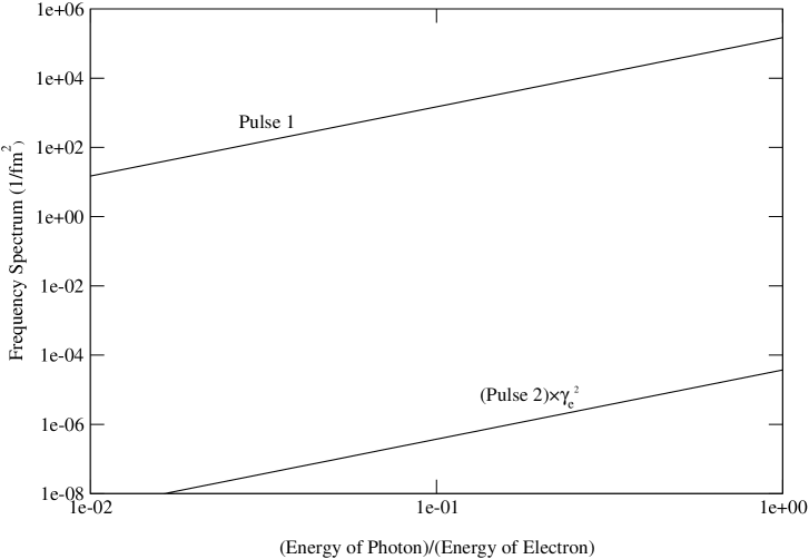
FIG. 7: Comparison of helicity-averaged frequency spectra of the three pulses of equivalent photons outside a 500 GeV electron. The helicity-averaged frequency spectrum, $\langle\mathrm{d}^{2}I/\mathrm{d}\omega\,\mathrm{d}A\rangle$, evaluated at the minimum impact parameter $b_{min}$, (cf. Eqs. (156a) – (156c)) is plotted on the y-axis and the Feynman scaling variable, $x=E_{\gamma}/E_{e}$, is plotted on the x-axis. Because the spectrum for Pulse 2, corresponding to transversely-polarized photons, is typically suppressed by a factor of $\gamma_{e}^{2}$ (which can be quite large) relative to that for Pulse 1, which also corresponds to transversely-polarized photons, it is shown here amplified by $\gamma_{e}^{2}$. Pulse 3, which corresponds to longitudinally-polarized photons, does not reveal itself on the graph because it vanishes everywhere, on account of the fact that longitudinally-polarized photons simply do not occur in nature.

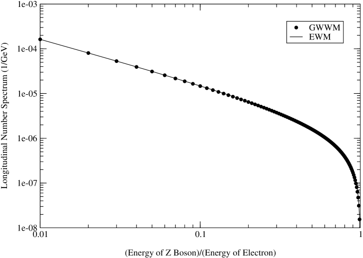
FIG. 13: Comparison of number spectra for longitudinally-polarized $Z$ bosons radiating from a 500 GeV electron. $N_{\mathrm{L}}$ is plotted on the y-axis and the Feynman scaling variable, $x=E_{Z}/E_{e}$, is plotted on the x-axis. The solid curve shows the predictions of the EWM and the dotted curve shows the results of the GWWM. Relative errors rise from 0% at $x=0$ to $7\%$ at $x=1$. There does not seem to be any dependence of the results on $E_{e}$, and only a slight dependence on $b_{min}$.

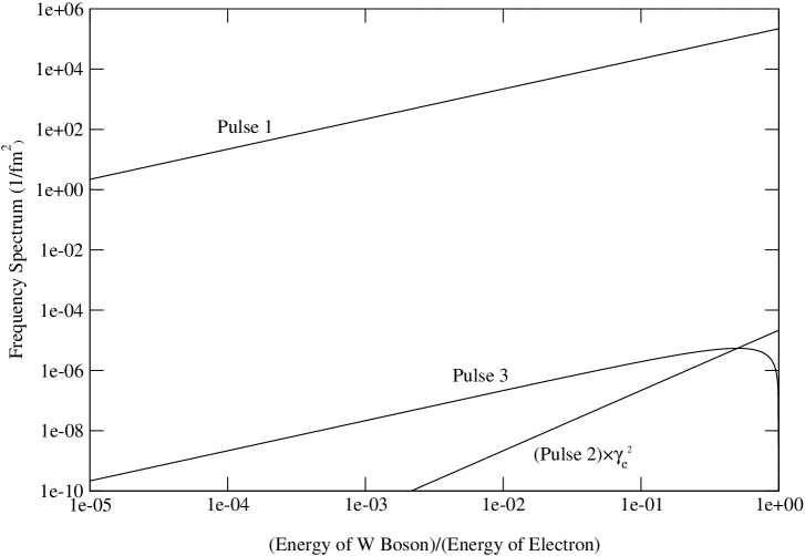
FIG. 16: Comparison of helicity-averaged frequency spectra of the three pulses of equivalent $W$ bosons outside a 500 GeV electron. The helicity-averaged frequency spectrum, $\langle\mathrm{d}^{2}I/\mathrm{d}\omega\,\mathrm{d}A\rangle$, evaluated at the minimum impact parameter $b_{min}$, (cf. Eqs. (156a) – (156c)) is plotted on the y-axis and the Feynman scaling variable, $x=E_{W}/E_{e}$, is plotted on the x-axis. Because the spectrum for Pulse 2, corresponding to transversely-polarized $W$ bosons, is typically suppressed by a factor of $\gamma_{e}^{2}$ (which can be quite large) relative to that for Pulse 1, which also corresponds to transversely-polarized $W$ bosons, it is shown here amplified by $\gamma_{e}^{2}$. Pulse 3 corresponds to the longitudinally-polarized $W$ bosons.

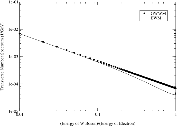
FIG. 17: Comparison of number spectra for transversely-polarized $W$ bosons radiating from a 500 GeV electron. $N_{\mathrm{T}}$ is plotted on the y-axis and the Feynman scaling variable, $x=E_{W}/E_{e}$, is plotted on the x-axis. The dotted curve shows the results of the GWWM and the solid curve shows the predictions of the EWM. Relative errors rise from $0\%$ at $x=0$ to $33\%$ at $x=1$. There does not seem to be any dependence of the results on $E_{e}$, but there is a strong dependence on $b_{min}$.

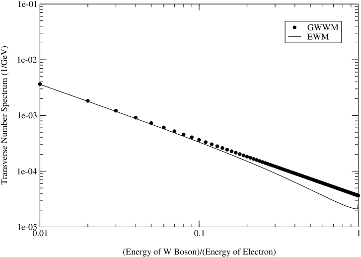
FIG. 18: Comparison of number spectra for transversely-polarized $W$ bosons radiating from a 1000 GeV electron. $N_{\mathrm{T}}$ is plotted on the y-axis and the Feynman scaling variable, $x=E_{W}/E_{e}$, is plotted on the x-axis. The dotted curve shows the results of the GWWM and the solid curve shows the predictions of the EWM. Relative errors rise from $0\%$ at $x=0$ to $33\%$ at $x=1$. There does not seem to be any dependence of the results on $E_{e}$, but there is a strong dependence on $b_{min}$.

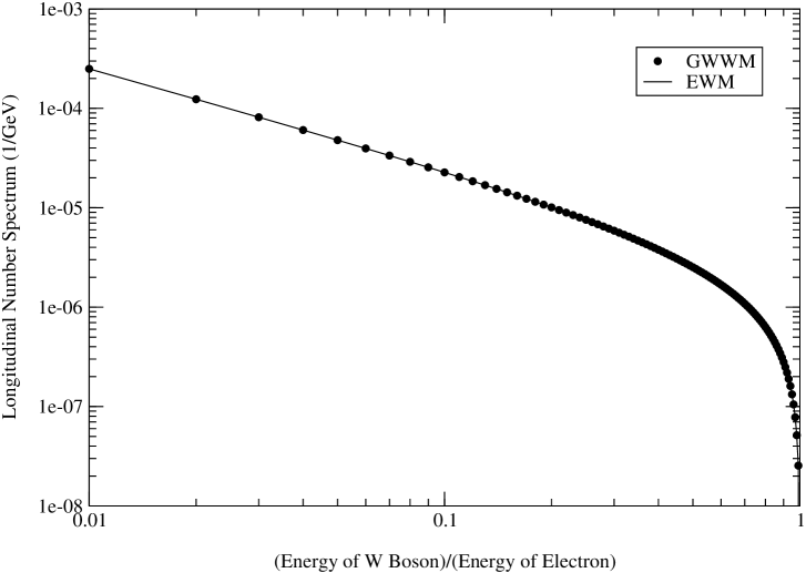
FIG. 19: Comparison of number spectra for longitudinally-polarized $W$ bosons radiating from a 500 GeV electron. $N_{\mathrm{L}}$ is plotted on the y-axis and the Feynman scaling variable, $x=E_{W}/E_{e}$, is plotted on the x-axis. The solid curve shows the predictions of the EWM and the dotted curve shows the results of the GWWM. Relative errors are always on the order of magnitude of $10^{-9}\,\%$, from $x=0$ to $x=1$. There is a slight dependence of the results on $E_{e}$ and $b_{min}$.

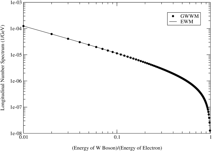
FIG. 20: Comparison of number spectra for longitudinally-polarized $W$ bosons radiating from a 1000 GeV electron. $N_{\mathrm{L}}$ is plotted on the y-axis and the Feynman scaling variable, $x=E_{W}/E_{e}$, is plotted on the x-axis. The solid curve shows the predictions of the EWM and the dotted curve shows the results of the GWWM. Relative errors are always on the order of magnitude of $10^{-8}\,\%$, from $x=0$ to $x=1$. There is a slight dependence of the results on $E_{e}$ and $b_{min}$.

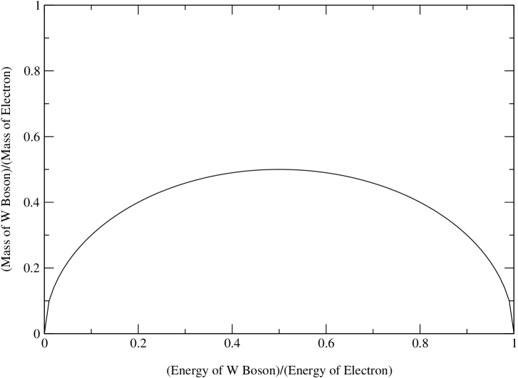
FIG. 21: The mass $m_{W}$ of an equivalent $W$ boson emitted from an electron. The ratio of $m_{W}$ to the mass $m_{e}$ of the electron is plotted on the y-axis and the Feynman scaling variable, $x=E_{W}/E_{e}$, is plotted on the x-axis. $m_{W}$ vanishes at $E_{W}=0$ and $E_{W}=E_{e}-m_{e}$, and peaks to a maximum value of $m_{e}/2$ at $E_{e}v_{e}/2$, where $v_{e}$ is the speed of the electron.

Results from this section (for bosons radiating from electrons) are shown in Figs. 7 – 21. Fig. 7 shows the helicity-averaged frequency spectra (cf. Eqs. (156a) – (156c)) for the three WW pulses of photons radiating from a 500 GeV electron. These functions generally depend on the boson energy $E_{b}$ as well as the impact parameter $b$. To only display the energy dependence, $b$ was set equal to the relevant minimum impact parameter, $b_{min}$. For a given $E_{b}$, this choice for $b$ gives the maximum value that the frequency spectra will take. Pulse 1, which represents transversely-polarized photons travelling collinearly with the electron, is by far the most dominant of the three pulses. Pulse 2, which is the fictitious pulse travelling in a direction transverse to the electron’s velocity, is relatively negligible; it is shown amplified by a factor of $\gamma_{e}^{2}$ so that it appears on the same graph as Pulse 1. Pulse 3, which represents longitudinally-polarized photons, does not appear at all on the graph because it vanishes altogether. The number spectra for transversely-polarized photons, as calculated via the GWWM (Eq. (1a)), or, equivalently, the SWWM (Eq. (12a)), is compared to the same function calculated via the QWWM (Eq. (20a)) in Fig. 8 and 9, for a particle accelerator operating at beam energies of 500 and 1000 GeV, respectively. For the 500 (1000) GeV electron case, the relative differences between the functions rise from $0\%$ at low photon energies to $169\%$ ($165\%$) at the highest possible photon energies. The helicity-averaged frequency spectra, evaluated at $b=b_{min}$, for the three pulses of equivalent $Z$ bosons ($W$ bosons) outside a 500 GeV electron are shown in Fig. 10 (Fig. 16). Like in the photon case, Pulse 1 exceeds Pulse 2 by a factor of at least $\gamma_{e}^{2}$, but unlike the photon case, Pulse 3, which describes longitudinally-polarized $Z$ bosons ($W$ bosons), is not completely negligible. Fig. 11 (Fig. 17) compares the number spectra for transversely-polarized $Z$ bosons ($W$ bosons) radiating from a 500 GeV electron, as calculated via the GWWM (Eq. (1a)), to the same function as calculated via the EWM (Eq. (23a)). Figs. 12 and 18 show the same comparisons for a collider operating at a beam energy of 1000 GeV. Relative discrepancies rise from $0\%$ at low boson energies to $33\%$ at high boson energies for both the $Z$ boson and $W$ boson, and both the 500 and 1000 GeV electron, cases. Fig. 13 (Fig. 19) compares the number spectra for longitudinally-polarized $Z$ bosons ($W$ bosons) radiating from a 500 GeV electron, as calculated via the GWWM (Eq. (1b)), to the same function as calculated via the EWM (Eq. (23b)). Figs. 14 and 20 show the same comparisons for a collider operating at a beam energy of 1000 GeV. For the $Z$ boson case, relative errors rise from $0\%$ at low boson energies to $7\%$ at high boson energies, for both a 500 and 1000 GeV electron. For the $W$ boson case, relative errors remain at a steady $10^{-9}\,\%$ and $10^{-8}\,\%$ for the 500 and 1000 GeV electrons, respectively, as $x$ varies from $0$ to $1$. The mass of an equivalent $Z$ or $W$ boson varies with the boson’s energy according to Eq. (8). This function is shown in Fig. 15 for $Z$ bosons and Fig. 21 for $W$ bosons.

To conclude, excellent agreement is found between the number spectrum functions of the GWWM and other theories, for bosons radiating from point particles. To achieve this agreement, the free parameter $\eta_{b}$ (first introduced in Eq. (154)) appearing in the GWWM is always found to be on the order of unity, as it is expected to be. When comparing the $N_{\mathrm{T}}$ for photons of the GWWM (i.e., the SWWM) to the same function in the QWWM, $\eta_{\gamma}$ is found to be $4\mathrm{e}^{-\gamma}=2.246$. And when comparing the $N_{\mathrm{T}}$ for massive bosons of the GWWM to the same function in the EWM, $\eta_{b}$ is found to be $4\mathrm{e}^{-(\gamma+1/2)}=1.362$. The $N_{\mathrm{L}}$ function for photons vanishes in both the GWWM (or the SWWM) and QWWM. The expression for $N_{\mathrm{L}}$ for massive bosons of the GWWM is found to be equal to that in the EWM in the $E_{b}\to 0$ limit, which has been pointed out previously is the limit of interest, and if $\alpha_{b}\simeq 1$, which turns out to be almost always the case.

5.6 Comparisons for Composite Particles

If the colliding particles are composite, the correct form for the minimum impact parameter in the GWWM is complicated. If the mediators are photons, Eq. (5) is used. As the GWWM simplifies to the well documented SWWM in this limit, the reader is referred to the literature on this subject. See [1], [4], [21], or any of the many papers by Baur, Bertulani, Greiner, or Soff, to name a few. In practice, the parameter $\eta_{f}$ appearing in Eq. (5) can simply be set to $1$, as $R_{1}+R_{2}$ is almost always (for applications to relativistic heavy ion colliders) much greater than $\eta_{f}/\gamma_{f}m_{f}v_{f}$. The focus thus turns to how the GWWM compares to the EWM when analyzing nucleus-nucleus collisions. The references on this subject are scarce, to say the least. One author who does calculate the number spectra for massive bosons emitted from heavy ions is Papageorgiu [27]. She uses the formulas of Kane et al., but in the opposite limit as was considered for applications to collisions between point particles [9]. That is, instead of evaluating the general equations in the $(p_{b\perp})_{max}\gg M_{b}$ limit, she evaluates them in the $(p_{b\perp})_{max}\ll M_{b}$ limit (cf. Eqs. (28a)–(28b)). Furthermore, she identifies $(p_{b\perp})_{max}$ with $1/R$, where $R$ is the radius of the parent nucleus, so the limit of interest can be written $M_{b}B_{min}\gg 1$, where $B_{min}=R$. Written this way, the number spectrum functions of interest are Eqs. (30a)–(30b). In view of the fact that $M_{b}B_{min}\gg 1$, the factor $\ln(1+1/M_{b}^{2}B_{min}^{2})$ in Eq. (30a) reduces to $1/M_{b}^{2}B_{min}^{2}$, and the factor $1/(1+M_{b}^{2}B_{min}^{2})$ in Eq. (30b) reduces to the same quantity, $1/M_{b}^{2}B_{min}^{2}$. The equations can be written

$$\lim_{E_{b}\to 0}\left\{[N_{\mathrm{T}}(E_{b})]_{EWM}\right\}\bigg{|}_{M_{b}B_{min}\gg 1} =\frac{N_{0}}{2E_{b}}\,\frac{1}{M_{b}^{2}B_{min}^{2}}$$ (39a)

$$\lim_{E_{b}\to 0}\left\{[N_{\mathrm{L}}(E_{b})]_{EWM}\right\}\bigg{|}_{M_{b}B_{min}\gg 1} =\frac{N_{0}}{2E_{b}}\,\frac{1}{M_{b}^{2}B_{min}^{2}}.$$ (39b)

Clearly, in these limits, $N_{\mathrm{T}}=N_{\mathrm{L}}$, which is pointed out by Papageorgiu. To compare the results of the GWWM with her results, first note that the correct expression to use for $b_{min}$ for such applications is given in Eq. (6). From this equation and the definition of $\chi_{b}$, it is apparent that

$$\chi_{b}=\frac{1}{2}b_{min}\Delta p_{b\perp}=\eta_{b}.$$ (40)

By the usual assumption that $\eta_{b}\sim 1$, it therefore follows that $\chi_{b}\sim 1$. By demanding that $\chi_{b}$ not be $\ll 1$ or $\gg 1$, the Bessel functions appearing in the expressions for $N_{\mathrm{T}}$ and $N_{\mathrm{L}}$ (cf. Eqs. (1a) and (1b)) do not simplify. But, if one considers the limit of interest, $E_{b}\to 0$, and recalls Eq. (149b), one finds $\Delta p_{b\perp}/2\to m_{b}$, so that $b_{min}$ can be written

$$b_{min}=\frac{\eta_{b}}{m_{b}},$$ (41)

which is the familiar relation relating the range of a force to the mass of the associated messenger boson. This equation can be rewritten as $m_{b}b_{min}=\eta_{b}$. It was just this quantity, $M_{b}B_{min}$, that Papageorgiu assumed was $\gg 1$; in comparison (and in contrast), again, it is assumed here that $m_{b}b_{min}\sim 1$. It is not too far-fetched, however, to allow $m_{b}b_{min}\gg 1$, or, equivalently, $\chi_{b}\gg 1$, here as well. A careful examination of a table of values of the modified Bessel functions appearing in the GWWM shows that the values of these functions evaluated at $\chi_{b}=1$ differ from their values in the $\chi_{b}\gg 1$ limits (cf. Eqs. (170a) and (170b)), also evaluated at $\chi_{b}=1$, by relative errors at only the 4% and 5% levels, respectively [45]. Allowing for the possibility that $\chi_{b}$ is somewhat greater than $1$ arrives at even better agreement. For instance, those relative errors are only 0.2% and 0.4%, respectively, when $\chi_{b}$ is set equal to $5$; and, they are both about 0.1% when $\chi_{b}$ is set equal to $10$. For the sake of simplicity, then, it is assumed here that $\chi_{b}\gg 1$ for applications of the method to nucleus-nucleus collisions. The values of $\chi_{b}$ that are ultimately found to work are between about $6$ and $9$, for all nuclei. So while this approximation is not in accord with the usual scenario, that $\eta_{b}\simeq 1$, it greatly simplifies the analysis, and arrives at very good results. With this limiting form for $\chi_{b}$, the appropriate limiting expressions for the GWWM number spectra are those listed in Eqs. (171f) and (172g). As in the case of applications to pointlike particles, the general procedure for finding an exact value of $\eta_{b}$ is to demand that the GWWM $N_{\mathrm{T}}$ and $N_{\mathrm{L}}$ functions in the low boson energy limit agree exactly with the same functions, in the same limit, appearing in Papageorgiu’s EWM-based analysis.

Consider first the $N_{\mathrm{T}}$ functions. As in the previous section, equate the expression for the GWWM $N_{\mathrm{T}}$ (found in Eq. (171f)) to a generic $N_{\mathrm{T}}$ function (to be identified with Eq. (39a) below).

$$\frac{\mathrm{\pi}}{4}\frac{N_{0}}{E_{b}}\,\mbox{\Large e}^{-2\chi_{b}} \equiv N_{\mathrm{T}}$$ (42a)

$$\mbox{\Large e}^{2\chi_{b}} =\frac{\mathrm{\pi}}{4}\frac{N_{0}}{N_{\mathrm{T}}E_{b}}$$ (42b)

$$2\chi_{b} =\log{\left(\frac{\mathrm{\pi}}{4}\frac{N_{0}}{N_{\mathrm{T}}E_{b}}\right)}$$ (42c)

$$\eta_{b} =\frac{1}{2}\,\log{\left(\frac{\mathrm{\pi}}{4}\frac{N_{0}}{N_{\mathrm{T}}E_{b}}\right)}\qquad\mbox{(via $\chi_{b}=\eta_{b}$).}$$ (42d)

Now, substitute Eq. (39a) for $N_{\mathrm{T}}$ here.

$$\eta_{b} =\frac{1}{2}\,\log{\left(\frac{\mathrm{\pi}}{2}M_{b}^{2}B_{min}^{2}\right)}$$ (43a)

$$=\log{\left(\sqrt{\frac{\mathrm{\pi}}{2}}M_{b}B_{min}\right)}$$ (43b)

$$=\log{\left(\sqrt{\frac{\mathrm{\pi}}{2}}M_{b}R\right)},$$ (43c)

where $B_{min}$ has been rewritten as $R$ (the nuclear radius) in the last line. An even more handy formula is found by substituting the known value for $R$, which is given in Eq. (159).

$$\eta_{b}=\log{\left(1.504M_{b}A^{1/3}\right)},$$ (44)

where the constant $1.504$ is more precisely $1.2\sqrt{\mathrm{\pi}/2}$. And, of course, $M_{b}$ is the on-shell value of the boson’s mass, and $A$ is the atomic mass of the nucleus that emits the boson. With $m_{W}=80.42$ GeV and $m_{Z}=91.19$ GeV, and considering values of $A$ to potentially range from $1$ (for hydrogen) to $238$ (for uranium), $\eta_{b}$ is found to range from a minimum of $6.418$ (for $W$ bosons radiating from protons) to a maximum of $8.368$ (for $Z$ bosons radiating from uranium nuclei) [16]. So, $\eta_{b}$ turns out to be closer (in order of magnitude) to $10$ than $1$. But, the use of the Heisenberg uncertainty principle is such an inherently tricky business to begin with that these values are not out of the realm of possibilities. Perhaps D. Griffiths put it best when he said, “In general, when you hear a physicist invoke the uncertainty principle, keep a hand on your wallet” [12].

The $N_{\mathrm{L}}$ functions are almost identical to the $N_{\mathrm{T}}$ functions in the limits of interest. Just as Papageorgiu found that $N_{\mathrm{T}}\simeq N_{\mathrm{L}}$, the $N_{\mathrm{L}}$ of Eq. (172g) is equal to the $N_{\mathrm{T}}$ of Eq. (171f) in the limit where $p_{f}\simeq E_{f}$, $E_{b}\ll E_{f}$, and $(1-\alpha_{b})E_{b}/\alpha_{b}E_{f}\ll 1$. The first two limits are the usual ones of interest. The third approximation holds in general, although there are exceptions (cf. Table 1 and the discussion thereafter); see also Eq. (38) and the discussion following it. So $N_{\mathrm{L}}\simeq N_{\mathrm{T}}$ in the GWWM, and since the $N_{\mathrm{T}}$ function of the GWWM is in excellent agreement with the $N_{\mathrm{T}}$ of Papageorgiu’s EWM-based analysis (which, again, $\simeq N_{\mathrm{L}}$ thereof), it is concluded that the above choice for $\eta_{b}$ simultaneously achieves good agreement between the $N_{\mathrm{L}}$ function of the GWWM and the $N_{\mathrm{L}}$ of Papageorgiu’s analysis.

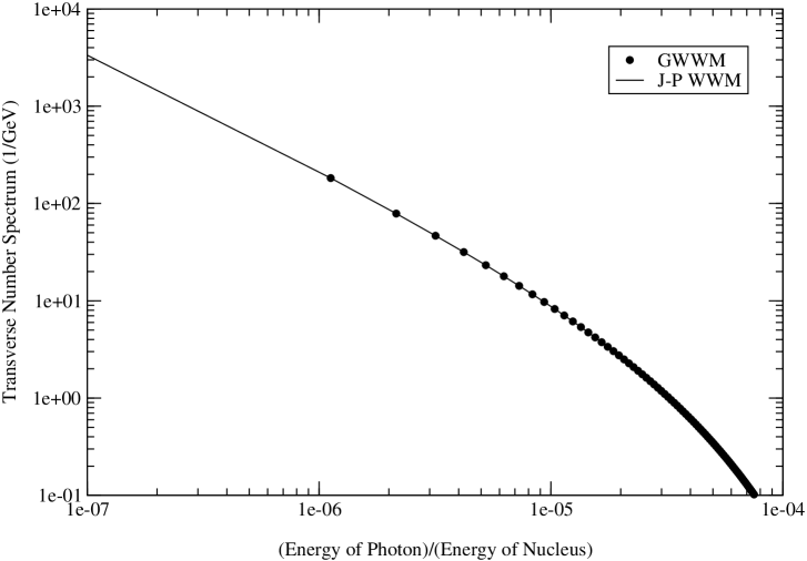
FIG. 23: Comparison of number spectra for transversely-polarized photons radiating from a lead (${}^{208}Pb$) nucleus at a relativistic heavy ion collider operating at a beam energy of $2.76\mathrm{A}$ TeV. Note that the number spectra for longitudinally-polarized photons always vanishes because photons are never found in longitudinal polarization states. $N_{\mathrm{T}}$ is plotted on the y-axis and the Feynman scaling variable, $x=E_{\gamma}/E_{nuc}$, is plotted on the x-axis. The dotted curve shows the results of the GWWM, which are also identically those of the SWWM, and the solid curve shows the predictions of the semiclassical version of the WWM developed by Jäckle and Pilkuhn [41]. Relative errors between the GWWM and the Jäckle-Pilkuhn WWM are always on the order of magnitude of $10^{-5}\,\%$, from $x=0$ to $x=1$. There does not seem to be any dependence of the results on $E_{nuc}$, but there is a strong dependence on $b_{min}$.

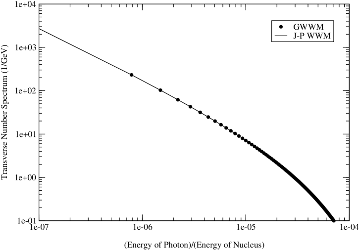
FIG. 24: Comparison of number spectra for transversely-polarized photons radiating from a lead (${}^{208}Pb$) nucleus at a relativistic heavy ion collider operating at a beam energy of $3.4\mathrm{A}$ TeV. Note that the number spectra for longitudinally-polarized photons always vanishes because photons are never found in longitudinal polarization states. $N_{\mathrm{T}}$ is plotted on the y-axis and the Feynman scaling variable, $x=E_{\gamma}/E_{nuc}$, is plotted on the x-axis. The dotted curve shows the results of the GWWM, which are also identically those of the SWWM, and the solid curve shows the predictions of the semiclassical version of the WWM developed by Jäckle and Pilkuhn [41]. Relative errors between the GWWM and the Jäckle-Pilkuhn WWM are always on the order of magnitude of $10^{-5}\,\%$, from $x=0$ to $x=1$. There does not seem to be any dependence of the results on $E_{nuc}$, but there is a strong dependence on $b_{min}$.

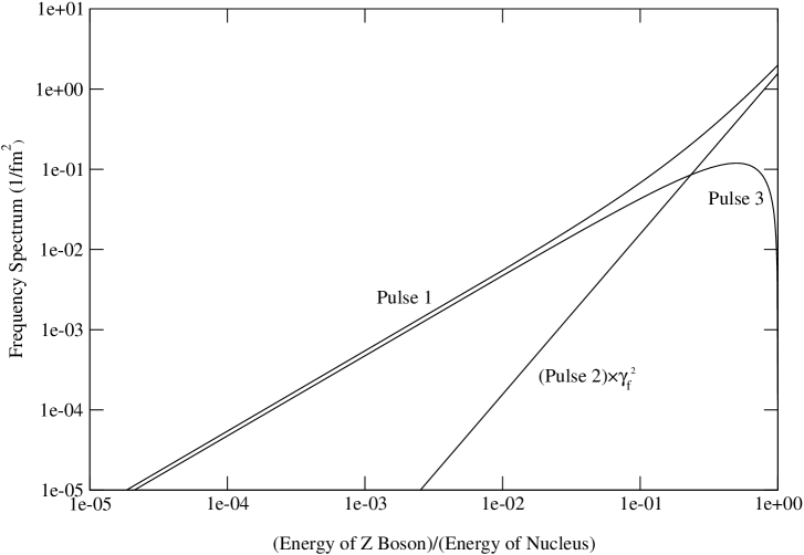
FIG. 25: Comparison of helicity-averaged frequency spectra of the three pulses of equivalent $Z$ bosons outside a lead (${}^{208}Pb$) nucleus at a relativistic heavy ion collider operating at a beam energy of $3.4\mathrm{A}$ TeV. The helicity-averaged frequency spectrum, $\langle\mathrm{d}^{2}I/\mathrm{d}\omega\,\mathrm{d}A\rangle$, evaluated at the minimum impact parameter $b_{min}$, (cf. Eqs. (156a) – (156c)) is plotted on the y-axis and the Feynman scaling variable, $x=E_{Z}/E_{f}$, is plotted on the x-axis. Because the spectrum for Pulse 2, corresponding to transversely-polarized $Z$ bosons, is typically suppressed by a factor of $\gamma_{f}^{2}$ (which can be quite large) relative to that for Pulse 1, which also corresponds to transversely-polarized $Z$ bosons, it is shown here amplified by $\gamma_{f}^{2}$. Pulse 3 corresponds to the longitudinally-polarized $Z$ bosons.

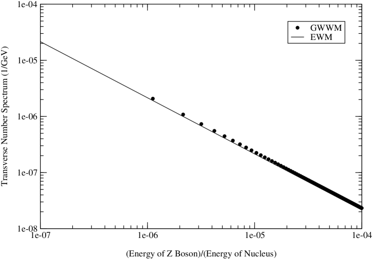
FIG. 26: Comparison of number spectra for transversely-polarized $Z$ bosons radiating from a lead (${}^{208}Pb$) nucleus at a relativistic heavy ion collider operating at a beam energy of $2.76\mathrm{A}$ TeV. $N_{\mathrm{T}}$ is plotted on the y-axis and the Feynman scaling variable, $x=E_{Z}/E_{nuc}$, is plotted on the x-axis. The dotted curve shows the results of the GWWM and the solid curve shows the predictions of the EWM. Relative errors are always about $8.4\%$, from $x=0$ to $x=1$. There does not seem to be any dependence of the results on $E_{nuc}$, but there is a strong dependence on $b_{min}$.

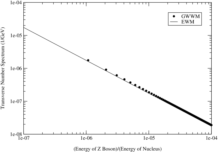
FIG. 27: Comparison of number spectra for transversely-polarized $Z$ bosons radiating from a lead (${}^{208}Pb$) nucleus at a relativistic heavy ion collider operating at a beam energy of $3.4\mathrm{A}$ TeV. $N_{\mathrm{T}}$ is plotted on the y-axis and the Feynman scaling variable, $x=E_{Z}/E_{nuc}$, is plotted on the x-axis. The dotted curve shows the results of the GWWM and the solid curve shows the predictions of the EWM. Relative errors are always about $8.4\%$, from $x=0$ to $x=1$. There does not seem to be any dependence of the results on $E_{nuc}$, but there is a strong dependence on $b_{min}$.

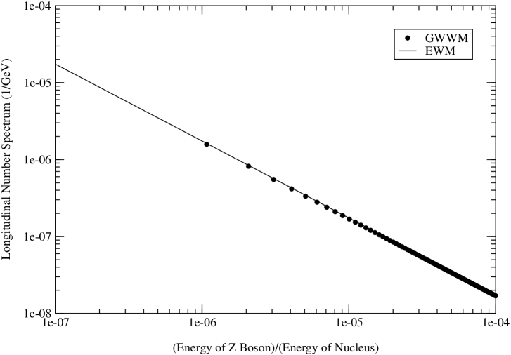
FIG. 29: Comparison of number spectra for longitudinally-polarized $Z$ bosons radiating from a lead (${}^{208}Pb$) nucleus at a relativistic heavy ion collider operating at a beam energy of $3.4\mathrm{A}$ TeV. $N_{\mathrm{L}}$ is plotted on the y-axis and the Feynman scaling variable, $x=E_{Z}/E_{nuc}$, is plotted on the x-axis. The solid curve shows the predictions of the EWM and the dotted curve shows the results of the GWWM. Relative errors are always about $2.7\%$, from $x=0$ to $x=1$. There does not seem to be any dependence of the results on $E_{nuc}$, but there is a strong dependence on $b_{min}$.

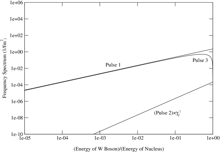
FIG. 31: Comparison of helicity-averaged frequency spectra of the three pulses of equivalent $W$ bosons outside a lead (${}^{208}Pb$) nucleus at a relativistic heavy ion collider operating at a beam energy of $3.4\mathrm{A}$ TeV. The helicity-averaged frequency spectrum, $\langle\mathrm{d}^{2}I/\mathrm{d}\omega\,\mathrm{d}A\rangle$, evaluated at the minimum impact parameter $b_{min}$, (cf. Eqs. (156a) – (156c)) is plotted on the y-axis and the Feynman scaling variable, $x=E_{W}/E_{f}$, is plotted on the x-axis. Because the spectrum for Pulse 2, corresponding to transversely-polarized $W$ bosons, is typically suppressed by a factor of $\gamma_{f}^{2}$ (which can be quite large) relative to that for Pulse 1, which also corresponds to transversely-polarized $Z$ bosons, it is shown here amplified by $\gamma_{f}^{2}$. Pulse 3 corresponds to the longitudinally-polarized $W$ bosons.

Results from this section (for bosons radiating from a composite particle) are shown in Figs. 22 – 36. Fig. 22 shows the helicity-averaged frequency spectra (cf. Eqs. (156a) – (156c)), evaluated at $b=b_{min}$, for the three WW pulses of photons radiating from a lead (${}^{208}Pb$) nucleus at a relativistic heavy ion collider operating at a beam energy of $3.4\mathrm{A}$ TeV. Pulse 1, which represents transversely-polarized photons travelling collinearly with the lead nucleus, is by far the most dominant of the three pulses. Pulse 2, which is the fictitious pulse travelling in a direction transverse to the nucleus’s velocity, is relatively negligible; it is shown multiplied by a factor of $\gamma_{f}^{2}$ so that it appears on the same graph as Pulse 1. Pulse 3, which represents longitudinally-polarized photons, does not appear at all on the graph because it vanishes altogether. The number spectra for transversely-polarized photons, as calculated via the GWWM (Eq. (1a)), or, equivalently, the SWWM (Eq. (12a)), is compared to the same function calculated via the version of the WWM developed by Jäckle and Pilkuhn (Eq. (19a)) in Figs. 23 and 24. The results shown in Fig. 23 are relevant to a collider operating at a beam energy of $2.76\mathrm{A}$ TeV, and those shown in Fig. 24 are relevant to beam energies of $3.4\mathrm{A}$ TeV, both energies of which will be characteristic of the LHC collider at CERN that is currently being upgraded [35, 16]. The relative differences between the functions are always about $10^{-5}\,\%$! The helicity-averaged frequency spectra, evaluated at $b=b_{min}$, for the three pulses of equivalent $Z$ bosons ($W$ bosons) outside a lead nucleus at a $3.4\mathrm{A}$ TeV relativistic heavy ion collider are shown in Fig. 25 (Fig. 31). Like in the photon case, Pulse 1 exceeds Pulse 2 by a factor of at least $\gamma_{f}^{2}$, but unlike the photon case, Pulse 3, which describes longitudinally-polarized $Z$ bosons ($W$ bosons), is nonnegligible, and, in fact, comparable to Pulse 1. Fig. 26 (Fig. 32) compares the number spectra for transversely-polarized $Z$ bosons ($W$ bosons) radiating from a lead nucleus at a $2.76\mathrm{A}$ TeV relativistic heavy ion collider, as calculated via the GWWM (Eq. (1a)), to the same function as calculated via the EWM (Eq. (23a)). Figs. 27 and 33 are similar graphs, but relevant to a $3.4\mathrm{A}$ TeV collider. Relative differences are always about $8.4\%$ ($8.5\%$) for all $Z$ boson ($W$ boson) energies. Fig. 28 (Fig. 34) compares the number spectra for longitudinally-polarized $Z$ bosons ($W$ bosons) radiating from a lead nucleus at a $2.76\mathrm{A}$ TeV relativistic heavy ion collider, as calculated via the GWWM (Eq. (1b)), to the same function as calculated via the EWM (Eq. (23b)). And Figs. 29 and 35 are similar graphs, but relevant to a $3.4\mathrm{A}$ TeV collider. For both the $Z$ boson and $W$ boson cases, relative errors are always about $2.7\%$. The mass of an equivalent $Z$ or $W$ boson varies with the boson’s energy according to Eq. (8). This function is shown in Fig. 30 for $Z$ bosons and Fig. 36 for $W$ bosons.

In summary, splendid agreement is found between the number spectrum functions of the GWWM and other theories, for bosons radiating from composite particles. To achieve this agreement, the free parameter $\eta_{b}$ (first introduced in Eq. (154)) appearing in the GWWM must be between $1$ and $10$. For applications to EM interactions, the value of $\eta_{b}$ is actually completely inconsequential. When comparing the $N_{\mathrm{T}}$ for massive bosons of the GWWM to the same function in the EWM, as applied to bosons radiating from a nucleus of atomic mass number $A$, $\eta_{b}$ is found to be $\log{\left(1.504M_{b}A^{1/3}\right)}$. This constant ranges from a minimum possible value of $6.418$ (for $W$ bosons radiating from protons) to a maximum possible value of $8.368$ (for $Z$ bosons radiating from uranium nuclei) [16]. The $N_{\mathrm{L}}$ function for photons vanishes in both the GWWM (or the SWWM) and the version of the WWM developed by Jäckle and Pilkuhn (Eq. (19b)). The expression for $N_{\mathrm{L}}$ for massive bosons of the GWWM is found to be equal to that in the EWM if, in addition to the above choice for $\eta_{b}$, $(1-\alpha_{b})E_{b}/\alpha_{b}E_{f}\ll 1$, or $\alpha_{b}\simeq 1$, which, as has been pointed out previously, generally holds true.

Chapter 6 Summary

In conclusion, an electroweak generalization of the semiclassical Weizsäcker-Williams Method was successfully developed. In particular, the number spectrum functions describing the distribution of massive and massless electroweak bosons swarming about an ultrarelativistic fermion were derived. As in the original method, the starting point for this derivation was the equation of motion: Maxwell’s equations for the massless photon case and the Proca equation for the massive $W$ and $Z$ boson cases. The relevant equation was solved for a point charge in relativistic motion. In all cases, the potentials and fields surrounding the moving charge were found to be highly Lorentz contracted in the plane transverse to the direction of motion. As in the original method, these potentials and fields were then approximated as pulses of plane wave radiation travelling collinearly with the moving charge. Fourier transforms of all quantities were taken to find the frequency spectra of these pulses of “equivalent bosons.” An integration over the wavefront area of the pulse and a division by the energy of the equivalent boson then yielded the number spectrum functions. These generalized functions differed in two ways from the original function that only pertained to massless photons. One was the charge of the fermion to which the boson couples and the other was the mass of the boson. The charges for each of the three types of electroweak interactions were derived from a knowledge of the corresponding fermion 4-current in a very straightforward way. All charges found were consistent with those appearing in the Standard Model. Values of the boson masses were obtained in a much more laborious manner. The main guiding principles behind this calculation were the conservation of energy and momentum, Lorentz invariance, and the concept of causality. The mass of a given equivalent boson was found to depend in a very specific way on the boson’s energy. These equivalent bosons are interpreted as being something analogous to off-shell SM boson states (i.e., virtual particles) that are tailor-made to fit the semiclassical method under consideration. The resulting number spectrum functions were compared to similar functions found in other theories. In all applications of the method, excellent agreement was obtained with other, more reliable, theories, proving the generalized Weizsäcker-Williams Method to be an accurate alternative to these more exact theories.

Appendix A: Electroweak 4-Currents

In this section, a formula for the 4-current $J^{\mu}(\boldsymbol{r},t)$ that is common to all three types of EW interactions of point charges is derived. Suppressing the $\boldsymbol{r}$ and $t$ dependence for notational simplicity, the fermion 4-currents appearing in the SM are generally of the form

$$J^{\mu}=g\bar{\psi}\tilde{\gamma}^{\mu}\tilde{Q}\psi,$$ (A.1)

where $g$ is the relevant coupling constant, $\psi$ is a fermion wave function (a solution to the Dirac equation (DE)), $\bar{\psi}$ is the Dirac adjoint of $\psi$, $\tilde{\gamma}^{\mu}$ is a Dirac matrix ( $\tilde{}$ denotes matrix), and $\tilde{Q}$ is the relevant charge operator.

The particular representation of the Dirac matrices that will be used here is the Weyl (or chiral) representation, where

$$\tilde{\gamma}^{0}=\begin{pmatrix}\;\;\;\tilde{0}&-\tilde{1}\\ -\tilde{1}&\;\;\;\tilde{0}\ \end{pmatrix}\quad\mbox{and}\quad\tilde{\gamma}^{\mathrm{i}}=\begin{pmatrix}\;\;\tilde{0}&\tilde{\sigma}^{\mathrm{i}}\\ -\tilde{\sigma}^{\mathrm{i}}&\tilde{0}\ \end{pmatrix}\qquad\mbox{(Dirac matrices).}$$ (A.2)

This representation facilitates splitting the fermion wave functions into definite chiral (right- and left-handed) eigenstates, which is how they naturally appear in the SM. It is to be understood that each element in Eq. (A.2) is actually a 2$\times$2 matrix. $\tilde{1}$ is thus the 2$\times$2 unit matrix, $\tilde{0}$ is the 2$\times$2 null matrix, and $\tilde{\sigma}^{\mathrm{i}}$ is the $\mathrm{i}^{th}$ Pauli spin matrix. The Pauli spin matrices are

$$\tilde{\sigma}^{1}=\begin{pmatrix}\;\,0&1\\ \;\,1&\;0\ \end{pmatrix}\mbox{,}\quad\tilde{\sigma}^{2}=\begin{pmatrix}\;\;\;0&-\mathrm{i}\\ -\mathrm{i}&\;\;\;\;0\ \end{pmatrix}\mbox{,}\quad\mbox{and}\quad\tilde{\sigma}^{3}=\begin{pmatrix}\;\,1&\;0\\ \;\,0&-1\ \end{pmatrix}$$

(Pauli spin matrices), (A.3)

where the elements this time are simply numbers. The following two relations are useful and easy to verify.

$$\tilde{\gamma}^{0}\tilde{\gamma}^{0}=\begin{pmatrix}\;\,\tilde{1}&\tilde{0}\\ \;\,\tilde{0}&\tilde{1}\ \end{pmatrix}\qquad\mbox{and}\qquad\tilde{\gamma}^{0}\tilde{\gamma}^{\mathrm{i}}=\begin{pmatrix}\;\,\tilde{\sigma}^{\mathrm{i}}&\tilde{0}\\ \;\,\tilde{0}&-\tilde{\sigma}^{\mathrm{i}}\ \end{pmatrix}.$$ (A.4)

They will be made use of later.

Having now specified the Dirac matrices, the Dirac adjoint $\bar{\psi}$ of $\psi$ can be related in a simple way to the more familiar Hermitian adjoint $\psi^{\dagger}$ of $\psi$:

$$\bar{\psi}=\psi^{\dagger}\tilde{\gamma}^{0}.$$ (A.5)

When all the whistles and bells are included, the fermion wave functions $\psi$ more generally appear in the form

$$\psi^{\mathrm{s}}_{\mathrm{c}}(x^{\mu},p^{\mu})=N\,\phi^{\mathrm{s}}_{\mathrm{c}}(p^{\mu})\,\mbox{\Large e}^{-\mathrm{i}p\cdot x}.$$ (A.6)

$\mathrm{s}$ labels the spin ($\mathrm{s}=1\,(2)$ for spin-up (down)); $\mathrm{c}$ labels the chirality ($\mathrm{c}=\mathrm{R}(\mathrm{L})$ for right (left) handed states, and is suppressed for nonchiral states); $x^{\mu}=(t,\boldsymbol{r})$ is the fermion’s 4-position; $p^{\mu}=(E,\boldsymbol{p})$ is the fermion’s 4-momentum; $N$ is a (real) normalization constant to be determined; and $\phi^{\mathrm{s}}_{\mathrm{c}}(p^{\mu})$ are 4-spinors which also satisfy the DE (solutions to the DE are always arbitrary up to a choice of normalization constant and overall phase factor). In a general Lorentz frame (and in the Weyl representation), the 4-spinors for a massive fermion are as follows.

$$\phi^{\mathrm{s}}_{\mathrm{R}}(p^{\mu})=\frac{1}{2\sqrt{m(E+m)}}\,\begin{bmatrix}(\tilde{E}+\tilde{m}+\tilde{\sigma}\cdot\boldsymbol{p})\tilde{\chi}^{\mathrm{s}}\\ \,\tilde{0}\ \end{bmatrix}$$ (A.7)

and

$$\phi^{\mathrm{s}}_{\mathrm{L}}(p^{\mu})=\frac{1}{2\sqrt{m(E+m)}}\,\begin{bmatrix}\tilde{0}\\ \,(\tilde{E}+\tilde{m}-\tilde{\sigma}\cdot\boldsymbol{p})\tilde{\chi}^{\mathrm{s}}\ \end{bmatrix},$$ (A.8)

where $m$ is the mass of the fermion, $\tilde{E}=\tilde{1}E$, $\tilde{m}=\tilde{1}m$, $\tilde{\sigma}\cdot\boldsymbol{p}=\tilde{\sigma}^{1}p_{x}+\tilde{\sigma}^{2}p_{y}+\tilde{\sigma}^{3}p_{z}$, and

$$\tilde{\chi}^{1}=\begin{pmatrix}1\\ \;\,0\ \end{pmatrix}\quad\mbox{and}\quad\tilde{\chi}^{2}=\begin{pmatrix}0\\ \;\,1\ \end{pmatrix}$$ (A.9)

are the basis spinors corresponding to spin-up (down) states [20, 13]. For arbitrary spins $\mathrm{s}$ and ${\mathrm{s}}^{\prime}$, the relation

$$\chi^{\mathrm{s}{\dagger}}\chi^{{\mathrm{s}}^{\prime}}=\delta_{ss^{\prime}},$$ (A.10)

where $\delta_{ss^{\prime}}$ is the Kronecker delta ($\delta_{ss^{\prime}}=1$ if $s=s^{\prime}$ and $\delta_{ss^{\prime}}0$ if $s\neq s^{\prime}$), is easily proved and very useful. Eqs. (A.7) and (A.8) represent four independent solutions to the DE for massive fermions. In the ultrarelativistic limit, where chirality is identical with helicity, these four solutions uniquely correspond to: a particle state with spin-up, a particle state with spin-down, an antiparticle state with spin-up, and an antiparticle state with spin-down. In a nonrelativistic limit, this description (in terms of particle and spin states) is less cut-and-dry. A nonchiral state $\phi^{\mathrm{s}}$ is simply the sum $\phi^{\mathrm{s}}_{\mathrm{R}}+\phi^{\mathrm{s}}_{\mathrm{L}}$:

$$\phi^{\mathrm{s}}(p^{\mu})\equiv\phi^{\mathrm{s}}_{\mathrm{R}}(p^{\mu})+\phi^{\mathrm{s}}_{\mathrm{L}}(p^{\mu})=\frac{1}{2\sqrt{m(E+m)}}\,\begin{bmatrix}(\tilde{E}+\tilde{m}+\tilde{\sigma}\cdot\boldsymbol{p})\tilde{\chi}^{\mathrm{s}}\\ \;(\tilde{E}+\tilde{m}-\tilde{\sigma}\cdot\boldsymbol{p})\tilde{\chi}^{\mathrm{s}}\ \end{bmatrix};$$ (A.11)

it is also a solution to the DE. In the rest frame limit ($E=m$ and $\boldsymbol{p}=\boldsymbol{0}$), it is easily deduced from Eqs. (A.7) and (A.8) that

$$\phi^{\mathrm{s}}_{\mathrm{R}}(p^{\mu})=\frac{1}{\sqrt{2}}\begin{bmatrix}\;\,\tilde{\chi}^{\mathrm{s}}\,\\ \;\,\tilde{0}\,\ \end{bmatrix}\quad\mbox{and}\quad\phi^{\mathrm{s}}_{\mathrm{L}}(p^{\mu})=\frac{1}{\sqrt{2}}\begin{bmatrix}\tilde{0}\\ \;\,\tilde{\chi}^{\mathrm{s}}\ \end{bmatrix}\qquad\mbox{(rest frame limit).}$$ (A.12)

Therefore,

$$\phi^{\mathrm{s}}(p^{\mu})\equiv\phi^{\mathrm{s}}_{\mathrm{R}}(p^{\mu})+\phi^{\mathrm{s}}_{\mathrm{L}}(p^{\mu})=\frac{1}{\sqrt{2}}\begin{bmatrix}\tilde{\chi}^{\mathrm{s}}\\ \;\,\tilde{\chi}^{\mathrm{s}}\ \end{bmatrix}\qquad\mbox{(rest frame limit),}$$ (A.13)

which is normalized to unity. In the massless limit, it is well-known that (for a particle, as opposed to an antiparticle, state)

$$\phi^{\mathrm{s}}_{\mathrm{R}}(p^{\mu})=\frac{1}{\sqrt{2}}\begin{bmatrix}\;\,\tilde{\chi}^{1}\,\\ \;\,\tilde{0}\,\ \end{bmatrix}\quad\mbox{and}\quad\phi^{\mathrm{s}}_{\mathrm{L}}(p^{\mu})=\frac{1}{\sqrt{2}}\begin{bmatrix}\tilde{0}\\ \;\,\tilde{\chi}^{2}\ \end{bmatrix}\qquad\mbox{(massless fermion),}$$ (A.14)

whence

$$\phi^{\mathrm{s}}(p^{\mu})\equiv\phi^{\mathrm{s}}_{\mathrm{R}}(p^{\mu})+\phi^{\mathrm{s}}_{\mathrm{L}}(p^{\mu})=\frac{1}{\sqrt{2}}\begin{bmatrix}\tilde{\chi}^{1}\\ \;\,\tilde{\chi}^{2}\ \end{bmatrix}\qquad\mbox{(massless fermion).}$$ (A.15)

The $\phi^{\mathrm{s}}_{\mathrm{R}}$ and $\phi^{\mathrm{s}}_{\mathrm{L}}$ 4-spinors have the property that they are eigenstates of the (normalized) helicity operator, with eigenvalues $+1$ and $-1$, respectively. A copious amount of experimental evidence indicates that neutrinos are nearly massless and are always left-handed [12, 13, 20]. For this reason, the $\phi^{\mathrm{s}}_{\mathrm{L}}$ wave functions are used in the SM to represent these fermions. The $\phi^{\mathrm{s}}_{\mathrm{R}}$ wave functions are then reserved for the antiparticle neutrino states. In short, the wave function specifications listed above are merely a statement that massless fermion particle states are always left-handed, and massless fermion antiparticle states are always right-handed.

The constant $N$ will now be determined for both massive and massless fermion wave functions, in the context of the probability 4-current. The probability 4-current $J^{P\mu}_{\mathrm{c}}$ associated with a solution $\psi^{\mathrm{s}}_{\mathrm{c}}$ of the DE is

$$J^{P\mu}_{\mathrm{c}}=\bar{\psi}^{\mathrm{s}}_{\mathrm{c}}\tilde{\gamma}^{\mu}\psi^{\mathrm{s}}_{\mathrm{c}}$$ (A.16)

[23, 13]. This 4-vector has the two main properties required of such a 4-current: the time component, to be interpreted as the probability density, is a scalar density that is positive definite,

$$J^{P0}_{\mathrm{c}}=\sum^{4}_{\mathrm{i}=1}\left|\left(\psi^{\mathrm{s}}_{\mathrm{c}}\right)_{\mathrm{i}}\right|^{2}>0;$$ (A.17)

and $J^{P\mu}_{\mathrm{c}}$ is conserved:

$$\partial^{\mu}J^{P}_{\mathrm{c}\mu}=0$$ (A.18)

[23]. Note that the summation index $\mathrm{i}$ in Eq. (A.17) runs over the four independent components of $\psi^{\mathrm{s}}_{\mathrm{c}}$ (equivalently, the four independent solutions to the DE), which can be easily identified in Eqs. (A.7)–(A.15). It is a well known result (Noether’s theorem) that if a 4-current is conserved (in the above sense), there is a corresponding conserved “charge” associated with it. This canonical charge is the integral of the $0$ component of the 4-current over an infinite spatial volume, evaluated on a hypersurface of constant time. For the case at hand, this charge $Q^{P}_{\mathrm{c}}$ is identified as the probability of finding the particle somewhere at some instant in time, as it is merely the volume integral of the probability density.

$$Q^{P}_{\mathrm{c}} =\lim_{V\to\infty}\int_{V}\mathrm{d}^{3}\boldsymbol{r}\,J^{P0}_{\mathrm{c}}$$ (A.19a)

$$=\lim_{V\to\infty}\int_{V}\mathrm{d}^{3}\boldsymbol{r}\,\bar{\psi}^{\mathrm{s}}_{\mathrm{c}}\tilde{\gamma}^{0}\psi^{\mathrm{s}}_{\mathrm{c}},\$$ (A.19b)

where it is to be understood that the integral is to be carried out on a hypersurface of constant time. Of interest to this study are point particles. So the given particle is confined to a given volume $V_{0}$, in the sense that $\psi^{\mathrm{s}}_{\mathrm{c}}$ is to be taken to vanish everywhere except inside $V_{0}$. Hence

$$Q^{P}_{\mathrm{c}} =\int_{V_{0}}\mathrm{d}^{3}\boldsymbol{r}\,\bar{\psi}^{\mathrm{s}}_{\mathrm{c}}\tilde{\gamma}^{0}\psi^{\mathrm{s}}_{\mathrm{c}}$$ (A.20a)

$$=\int_{V_{0}}\mathrm{d}^{3}\boldsymbol{r}\,N^{2}\bar{\phi}^{\mathrm{s}}_{\mathrm{c}}\tilde{\gamma}^{0}\phi^{\mathrm{s}}_{\mathrm{c}}$$ (A.20b)

$$=\int_{V_{0}}\mathrm{d}^{3}\boldsymbol{r}\,N^{2}\phi^{\mathrm{s}{\dagger}}_{\mathrm{c}}\tilde{\gamma}^{0}\tilde{\gamma}^{0}\phi^{\mathrm{s}}_{\mathrm{c}}$$ (A.20c)

$$=V_{0}N^{2}\phi^{\mathrm{s}{\dagger}}_{\mathrm{c}}\phi^{\mathrm{s}}_{\mathrm{c}}.\$$ (A.20d)

This last step follows from the facts that $\tilde{\gamma}^{0}\tilde{\gamma}^{0}=\tilde{1}$, and $N$ and $\phi^{\mathrm{s}}_{\mathrm{c}}$ are independent of $\boldsymbol{r}$ (in any Lorentz frame). Since $Q^{P}_{\mathrm{c}}$ is Lorentz invariant (by Noether’s theorem), it need only be evaluated in the particle’s own rest frame. Of course this step can only be done in the case of massive fermions. For the massless case, the following analysis can be performed in an arbitrary Lorentz frame, and all results can be shown to agree with those for the massive case. One need only keep in mind that $\mathrm{s}=2$ ($\mathrm{s}=1$) for $R$ ($L$) chiral states (via Eq. (A.14)). Assuming this to be the case, then, the following will only be concerned with massive fermions. In the rest frame of a massive fermion (recall Eqs. (A.12) and (A.13)),

$$\phi^{\mathrm{s}{\dagger}}_{\mathrm{R}}\phi^{\mathrm{s}}_{\mathrm{R}} =\frac{1}{2}\left[\tilde{\chi}^{\mathrm{s}{\dagger}},\tilde{0}\right]\begin{bmatrix}\;\;\tilde{\chi}^{\mathrm{s}}\;\\ \;\;\tilde{0}\;\ \end{bmatrix}=\frac{1}{2}\tilde{\chi}^{\mathrm{s}{\dagger}}\tilde{\chi}^{\mathrm{s}}=\frac{1}{2},$$ (A.21a)

$$\phi^{\mathrm{s}{\dagger}}_{\mathrm{L}}\phi^{\mathrm{s}}_{\mathrm{L}} =\frac{1}{2}\left[\tilde{0},\tilde{\chi}^{\mathrm{s}{\dagger}}\right]\begin{bmatrix}\tilde{0}\\ \;\;\tilde{\chi}^{\mathrm{s}}\ \end{bmatrix}=\frac{1}{2}\tilde{\chi}^{\mathrm{s}{\dagger}}\tilde{\chi}^{\mathrm{s}}=\frac{1}{2},\quad\mbox{and}$$ (A.21b)

$$\phi^{\mathrm{s}{\dagger}}\phi^{\mathrm{s}} =\frac{1}{2}\left[\tilde{\chi}^{\mathrm{s}{\dagger}},\tilde{\chi}^{\mathrm{s}{\dagger}}\right]\begin{bmatrix}\tilde{\chi}^{\mathrm{s}}\\ \;\tilde{\chi}^{\mathrm{s}}\ \end{bmatrix}=\frac{1}{2}\left(\tilde{\chi}^{\mathrm{s}{\dagger}}\tilde{\chi}^{\mathrm{s}}+\tilde{\chi}^{\mathrm{s}{\dagger}}\tilde{\chi}^{\mathrm{s}}\right)=1.\$$ (A.21c)

So

$$Q^{P}_{\mathrm{R}}=Q^{P}_{\mathrm{L}}=\frac{1}{2}V_{0}N^{2}$$ (A.22)

and

$$Q^{P}=Q^{P}_{\mathrm{R}}+Q^{P}_{\mathrm{L}}=V_{0}N^{2}.$$ (A.23)

It is reasonable to interpret these results to mean that a massive fermion is equally likely to be found in a right handed or left handed state. In the case where the fermion is massless, this statement is still true, since a fermion particle state is always left handed, while the antiparticle state of the same fermion is always right handed. Setting $Q^{P}\equiv 1$, which says that (if found) there is a 100% chance that the fermion will be found in one of either of these two mutually exclusive states. Then $Q^{P}_{\mathrm{R}}=Q^{P}_{\mathrm{L}}=1/2$ and

$$N=\frac{1}{\sqrt{V_{0}}}.$$ (A.24)

As stipulated, $N$ is independent of $\boldsymbol{r}$. Also, as mentioned above, the same result can easily be obtained in the case where the fermion is massless. For simplicity, all particles in this thesis are to be regarded as pointlike. This constraint is made quantitative by considering the limit of Eq. (A.24) as $V_{0}\to 0$. In this limit, $1/V_{0}$ (centered on the particle with 4-position $x^{\mu}=(t,\boldsymbol{r})$) becomes a Dirac delta function $\delta[\boldsymbol{r}(t)]$, and

$$N\to\lim_{V_{0}\to 0}\sqrt{\frac{1}{V_{0}}}=\sqrt{\delta[\boldsymbol{r}(t)]}.$$ (A.25)

The wave function becomes

$$\psi^{\mathrm{s}}_{\mathrm{c}}(x^{\mu},p^{\mu})=\sqrt{\delta[\boldsymbol{r}(t)]}\,\phi^{\mathrm{s}}_{\mathrm{c}}(p^{\mu})\,\mbox{\Large e}^{-\mathrm{i}p\cdot x}.$$ (A.26)

It is this form that shall henceforth be adopted as the wave function of any particle (massive or not) appearing in this thesis.

A word about the choice of normalization constant $N$ is in order. The choice for $N$ specified in Eq. (A.24) is referred to as “box normalization”; it is used extensively in nonrelativistic quantum mechanics and occasionally in relativistic quantum mechanics. [14, 23, 28, 47]. For example, a common problem encountered in nonrelativistic quantum mechanics is that of determining the energy spectrum of a particle confined to an infinite one dimensional square-well potential (a “box”), say, centered at $x=0$ and having width $L$. In this example, $L$ is a one dimensional version of the $V_{0}$ introduced above. By construction, the particle’s wave function (the momentum eigenfunction) $\Psi(x)$ vanishes at the boundaries of the box (i.e., $\Psi(-L/2)=\Psi(L/2)=0$), so all relevant integrals are like those in Eqs. (A.20a)–(A.20d), in the sense that only the region of space within length $L$ is of interest. In this particular example, $\Psi(x)$ is known to generally be of the form

$$\Psi(x)=N\mbox{\Large e}^{\mathrm{i}k_{x}x},$$ (A.27)

for $|x|\leq L/2$, and $\Psi(x)=0$ everywhere outside the box, where $k_{x}$ is the particle’s momentum, and $N$ is the normalization constant to be determined. $N$ is deduced in the same spirit as was done above: by normalizing $\Psi(x)$ so that the probability of finding the particle between $x=-L/2$ and $x=+L/2$ is exactly one. One finds (see, [28], for example)

$$1 =\int_{-L/2}^{+L/2}\mathrm{d}x\,{\Psi}^{\ast}(x)\Psi(x)$$ (A.28a)

$$=N^{2}\int_{-L/2}^{+L/2}\mathrm{d}x\,\mbox{\Large e}^{-\mathrm{i}{k^{\prime}}_{x}x}\mbox{\Large e}^{\mathrm{i}k_{x}x}$$ (A.28b)

$$=N^{2}\int_{-L/2}^{+L/2}\mathrm{d}x\,\mbox{\Large e}^{\mathrm{i}(k_{x}-{k^{\prime}}_{x})x}$$ (A.28c)

$$=N^{2}\left(L\,\delta_{k_{x}{k^{\prime}}_{x}}\right),$$ (A.28d)

where $\delta_{k_{x}{k^{\prime}}_{x}}$ is the Kronecker delta function. Since $k_{x}={k^{\prime}}_{x}$, it follows, therefore, that $N=1/\sqrt{L}$. If the particle’s wave function does not vanish on some given boundary, but is still described by Eq. (A.27), an alternative normalization constant is deduced. In this case, the above limits of integration are $\pm\infty$, instead of $\pm L/2$, respectively. The appropriate orthonormality relation for $\Psi(x)$ on the $x=(-\infty,\,+\infty)$ interval is

$$\delta(k_{x}-{k^{\prime}}_{x}) =\int_{-\infty}^{+\infty}\mathrm{d}x\,{\Psi}^{\ast}(x)\Psi(x)$$ (A.29a)

$$=N^{2}\int_{-\infty}^{+\infty}\mathrm{d}x\,\mbox{\Large e}^{-\mathrm{i}{k^{\prime}}_{x}x}\mbox{\Large e}^{\mathrm{i}k_{x}x}$$ (A.29b)

$$=N^{2}\int_{-\infty}^{+\infty}\mathrm{d}x\,\mbox{\Large e}^{\mathrm{i}(k_{x}-{k^{\prime}}_{x})x}$$ (A.29c)

$$=N^{2}\left[2\mathrm{\pi}\,\delta(k_{x}-{k^{\prime}}_{x})\right],$$ (A.29d)

where $\delta(k_{x}-{k^{\prime}}_{x})$ is the usual Dirac delta function. Thus, $N=1/\sqrt{2\mathrm{\pi}}$ for these cases. These prototypical normalization constants are easily found to generalize to $N=1/L^{3/2}$ (or $N=1/\sqrt{V_{0}}$, where $V_{0}=L^{3}$) and $N=1/({2\mathrm{\pi}})^{3/2}$, respectively, in three dimensions. In short, $N=1/\sqrt{V_{0}}$ is used in cases where the particle’s wave function is known to vanish on the boundary of some volume $V_{0}$, and $N=1/({2\mathrm{\pi}})^{3/2}$ is used in cases where there is no sharp discontinuity imposed on $\Psi(x)$. An example of where the latter type of normalization constant might be used is in the wave function describing a plane-wave wave packet freely propagating through empty space. It is also used extensively in relativistic quantum mechanics (in second quantization), where all operators are expressed as infinite sums of plane wave states. In this thesis, it is assumed for simplicity that all fermions of interest are very localized. As such, the $N=1/\sqrt{V_{0}}$ is the more appropriate normalization constant to use. The obvious question then arises as to what volume $V_{0}$ to use. To avoid this whole issue, another simplifying assumption is made: the wave functions are defined in the limit where $V_{0}\to 0$, Eq. (A.25). By taking this limit, the particles are being envisioned as ideally pointlike, in the sense of having a vanishing spatial dimension. Many authors use the box normalization, $N=1/\sqrt{V_{0}}$, but few, if any, impose this additional “point particle constraint”. The reason for this is probably twofold. One is that, if particles are being treated as pointlike, the more obvious route of analysis is that of second quantization, which uses the $N=1/({2\mathrm{\pi}})^{3/2}$ choice (as mentioned above), because quantum field theory is invariably more accurate than such a classical approach as taken here. Another reason might be that such a point particle approximation is not always needed; it is not terribly difficult (see, e.g., Sec. 4.2) to make reasonable approximations about the density profile of an elementary particle. The delta function approximation is done here merely for simplicity. In particular, the fermion 4-potential $A^{\mu}$ depends on an integral of the fermion 4-current $J^{\mu}$ (cf. Eq. (9)). By taking $N=\sqrt{\delta[\boldsymbol{r}(t)]}$ instead of $N=1/\sqrt{V_{0}}$, a $J^{\mu}$ is obtained that depends on $\delta[\boldsymbol{r}(t)]$ instead of some $1/V_{0}$, which considerably simplifies the expression: the delta function kills the integral entirely, and the expression for $A^{\mu}$ reduces to a very compact formula! In summary, the choice of box normalization (Eq. A.24) is merely one of at least two possible conventional choices to make. The subsequent delta function approximation made here (Eq. A.25) is not a conventional step to take, but it is very reasonable, and considerably simplifies the analysis (in particular, the evaluation of Eq. (9)).

It will prove useful later to have explicit expressions for the two probability 4-currents $J^{P\mu}_{\mathrm{R}}$ and $J^{P\mu}_{\mathrm{L}}$. So, at the risk of digressing for a while, attention is now turned to this derivation. These 4-currents will first be derived in a frame comoving with the particle. As mentioned before, this line of attack cannot be performed for massless fermions, as there is no such Lorentz frame for such particles. For those cases, the analysis is to be carried out in an arbitrary Lorentz frame, and all intermediate steps can be easily shown to be identical with those arrived at in the massive fermion case. Also, two constraints will be imposed on the system for simplicity. One is that 4-momentum is to be conserved in going from the initial to the final fermion states. The other is that the limit of the time duration between the initial and final fermion states is to be taken to go to zero. Under these conditions, Eq. (A.16), with Eq. (A.26) for $\psi^{\mathrm{s}}_{\mathrm{c}}$, becomes

$${J^{P\mu}}^{\prime}_{\mathrm{c}}=\delta[\boldsymbol{r^{\prime}}(t^{\prime})]\left[\bar{\phi}^{\mathrm{s}}_{\mathrm{c}}({p^{\mu}}^{\prime})\mbox{\Large e}^{+\mathrm{i}mt^{\prime}}\right]\tilde{\gamma}^{\mu}\left[\phi^{\mathrm{s}}_{\mathrm{c}}({p^{\mu}}^{\prime})\mbox{\Large e}^{-\mathrm{i}mt^{\prime}}\right].$$ (A.30)

Primed quantities are those measured relative to the rest frame of the fermion, so that ${p^{\mu}}^{\prime}=(m,\boldsymbol{0})$ and ${x^{\mu}}^{\prime}=(t^{\prime},\boldsymbol{0})$, where $t^{\prime}$ is the fermion’s proper time. Eq. (A.30) can be simplified a few steps further before special cases must be considered.

$${J^{P\mu}}^{\prime}_{\mathrm{c}} =\delta[\boldsymbol{r^{\prime}}(t^{\prime})]\bar{\phi}^{\mathrm{s}}_{\mathrm{c}}({p^{\mu}}^{\prime})\tilde{\gamma}^{\mu}\phi^{\mathrm{s}}_{\mathrm{c}}({p^{\mu}}^{\prime})$$ (A.31a)

$$=\delta[\boldsymbol{r^{\prime}}(t^{\prime})]\phi^{\mathrm{s}{\dagger}}_{\mathrm{c}}({p^{\mu}}^{\prime})\tilde{\gamma}^{0}\tilde{\gamma}^{\mu}\phi^{\mathrm{s}}_{\mathrm{c}}({p^{\mu}}^{\prime}).$$ (A.31b)

Using Eqs. (A.4) and (A.12), the $0$ components of the $R$, $L$, and nonchiral probability 4-currents (in the particle’s rest frame) are as follows.

$${J^{P0}}^{\prime}_{\mathrm{R}} =\delta[\boldsymbol{r^{\prime}}(t^{\prime})]\frac{1}{2}\left[\tilde{\chi}^{\mathrm{s}{\dagger}},\tilde{0}\right]\begin{bmatrix}\;\;\tilde{\chi}^{\mathrm{s}}\;\\ \;\;\tilde{0}\;\ \end{bmatrix}$$ (A.32a)

$$=\frac{1}{2}\delta[\boldsymbol{r^{\prime}}(t^{\prime})].$$ (A.32b)

$${J^{P0}}^{\prime}_{\mathrm{L}} =\delta[\boldsymbol{r^{\prime}}(t^{\prime})]\frac{1}{2}\left[\tilde{0},\tilde{\chi}^{\mathrm{s}{\dagger}}\right]\begin{bmatrix}\tilde{0}\\ \;\;\tilde{\chi}^{\mathrm{s}}\ \end{bmatrix}$$ (A.32c)

$$=\frac{1}{2}\delta[\boldsymbol{r^{\prime}}(t^{\prime})].$$ (A.32d)

${J^{P0}}^{\prime}$ is simply the sum of these two quantities:

$${J^{P0}}^{\prime} ={J^{P0}}^{\prime}_{\mathrm{R}}+{J^{P0}}^{\prime}_{\mathrm{L}}$$ (A.33a)

$$=\frac{1}{2}\delta[\boldsymbol{r^{\prime}}(t^{\prime})]+\frac{1}{2}\delta[\boldsymbol{r^{\prime}}(t^{\prime})]$$ (A.33b)

$$=\delta[\boldsymbol{r^{\prime}}(t^{\prime})].$$ (A.33c)

The vector components can be found with the aid of Eq. (A.4).

$${J^{P\mathrm{i}}}^{\prime}_{\mathrm{R}} =\delta[\boldsymbol{r^{\prime}}(t^{\prime})]\frac{1}{2}\left[\tilde{\chi}^{\mathrm{s}{\dagger}},\tilde{0}\right]\begin{pmatrix}\;\,\tilde{\sigma}^{\mathrm{i}}&\tilde{0}\\ \;\,\tilde{0}&-\tilde{\sigma}^{\mathrm{i}}\ \end{pmatrix}\begin{bmatrix}\;\;\tilde{\chi}^{\mathrm{s}}\;\\ \;\;\tilde{0}\;\ \end{bmatrix}$$ (A.34a)

$$=\frac{1}{2}\delta[\boldsymbol{r^{\prime}}(t^{\prime})]\left[\tilde{\chi}^{\mathrm{s}{\dagger}},\tilde{0}\right]\begin{bmatrix}\;\;\tilde{\sigma}^{\mathrm{i}}\tilde{\chi}^{\mathrm{s}}\;\\ \;\;\tilde{0}\;\ \end{bmatrix}$$ (A.34b)

$$=\frac{1}{2}\delta[\boldsymbol{r^{\prime}}(t^{\prime})]\left(\tilde{\chi}^{\mathrm{s}{\dagger}}\tilde{\sigma}^{\mathrm{i}}\tilde{\chi}^{\mathrm{s}}\right).$$ (A.34c)

The only nonvanishing component here is ${J^{P3}}^{\prime}_{\mathrm{R}}$, corresponding to the spin oriented along the $z$ axis (recall $\tilde{\chi}^{s}$ are eigenvectors of $\tilde{S}^{3}=\tilde{\sigma}^{3}/2$, with eigenvalues $\pm 1/2$ for spin up (down)). Define $\boldsymbol{\hat{s}}$ as the direction of the particle’s spin, so that $\boldsymbol{\hat{s}}=\pm\boldsymbol{\hat{z}}$ is identified with $\mathrm{s}=1(2)$, or spin up (down). Then

$${\boldsymbol{J}^{P}}^{\prime}_{\mathrm{R}} =\frac{1}{2}\delta[\boldsymbol{r^{\prime}}(t^{\prime})]\boldsymbol{\hat{s}}$$ (A.35a)

$$=\frac{1}{2}\delta[\boldsymbol{r^{\prime}}(t^{\prime})]{\boldsymbol{S}}^{\prime},$$ (A.35b)

where ${\boldsymbol{S}}^{\prime}$ is the vector component of the particle’s normalized 4-spin $s^{\mu}$ in its own rest frame. In the rest frame of the particle, $s^{\mu}$ given as ${s^{\mu}}^{\prime}=(0,{\boldsymbol{S}}^{\prime})\equiv(0,\boldsymbol{\hat{s}})$ (i.e., $s^{\mu}$ is a 4-vector that reduces to the particle’s normalized spin $\boldsymbol{\hat{s}}$ in its own rest frame). A similar result is found for ${\boldsymbol{J}^{P}}^{\prime}_{\mathrm{L}}$:

$${J^{P\mathrm{i}}}^{\prime}_{\mathrm{L}} =\delta[\boldsymbol{r^{\prime}}(t^{\prime})]\frac{1}{2}\left[\tilde{0},\tilde{\chi}^{\mathrm{s}{\dagger}}\right]\begin{pmatrix}\;\,\tilde{\sigma}^{\mathrm{i}}&\tilde{0}\\ \;\,\tilde{0}&-\tilde{\sigma}^{\mathrm{i}}\ \end{pmatrix}\begin{bmatrix}\tilde{0}\\ \;\;\tilde{\chi}^{\mathrm{s}}\ \end{bmatrix}$$ (A.36a)

$$=\frac{1}{2}\delta[\boldsymbol{r^{\prime}}(t^{\prime})]\left[\tilde{0},\tilde{\chi}^{\mathrm{s}{\dagger}}\right]\begin{bmatrix}\;\;\;\tilde{0}\\ \;\,-\tilde{\sigma}^{\mathrm{i}}\tilde{\chi}^{\mathrm{s}}\;\ \end{bmatrix}$$ (A.36b)

$$=-\frac{1}{2}\delta[\boldsymbol{r^{\prime}}(t^{\prime})]\left(\tilde{\chi}^{\mathrm{s}{\dagger}}\tilde{\sigma}^{\mathrm{i}}\tilde{\chi}^{\mathrm{s}}\right).$$ (A.36c)

Thus

$${\boldsymbol{J}^{P}}^{\prime}_{\mathrm{L}} =-\frac{1}{2}\delta[\boldsymbol{r^{\prime}}(t^{\prime})]\boldsymbol{\hat{s}}$$ (A.37a)

$$=-\frac{1}{2}\delta[\boldsymbol{r^{\prime}}(t^{\prime})]{\boldsymbol{S}}^{\prime}.$$ (A.37b)

Finally,

$${\boldsymbol{J}^{P}}^{\prime} ={\boldsymbol{J}^{P}}^{\prime}_{\mathrm{R}}+{\boldsymbol{J}^{P}}^{\prime}_{\mathrm{L}}$$ (A.38a)

$$=\frac{1}{2}\delta[\boldsymbol{r^{\prime}}(t^{\prime})]{\boldsymbol{S}}^{\prime}-\frac{1}{2}\delta[\boldsymbol{r^{\prime}}(t^{\prime})]{\boldsymbol{S}}^{\prime}$$ (A.38b)

$$=\boldsymbol{0}.$$ (A.38c)

The results of this paragraph can be summarized in a very simple set of equations. Introduce the 4-velocity $u^{\mu}$ and normalized 4-spin $s^{\mu}$ of the particle. In the rest frame of the particle, ${u^{\mu}}^{\prime}=(1,\boldsymbol{0})$ and ${s^{\mu}}^{\prime}=(0,\boldsymbol{\hat{s}})$, where $\boldsymbol{\hat{s}}=\pm\boldsymbol{\hat{z}}$ for spin up (down), as mentioned above. For a frame in which the particle moves with velocity $\boldsymbol{v}=v\boldsymbol{\hat{z}}$, these 4-vectors transform (under basic Lorentz transformations) into $u^{\mu}=\gamma(1,\boldsymbol{v})$ and $s^{\mu}=\gamma(v\boldsymbol{\hat{s}}\cdot\boldsymbol{\hat{z}},\boldsymbol{\hat{s}})$. In the rest frame,

$$\left.\begin{array}[]{r@{\, = \;}l}{J^{P\mu}}^{\prime}_{\mathrm{R}}&\frac{1}{2}\delta[\boldsymbol{r^{\prime}}(t^{\prime})](1,\boldsymbol{\hat{s}})=\frac{1}{2}\delta[\boldsymbol{r^{\prime}}(t^{\prime})]({u^{\mu}}^{\prime}+{s^{\mu}}^{\prime})\\ {J^{P\mu}}^{\prime}_{\mathrm{L}}&\frac{1}{2}\delta[\boldsymbol{r^{\prime}}(t^{\prime})](1,-\boldsymbol{\hat{s}})=\frac{1}{2}\delta[\boldsymbol{r^{\prime}}(t^{\prime})]({u^{\mu}}^{\prime}-{s^{\mu}}^{\prime})\\ {J^{P\mu}}^{\prime}&\delta[\boldsymbol{r^{\prime}}(t^{\prime})](1,\boldsymbol{0})=\delta[\boldsymbol{r^{\prime}}(t^{\prime})]{u^{\mu}}^{\prime}\\ \end{array}\right\}\qquad\mbox{(rest frame).}$$ (A.39)

In a moving frame, the forms of these 4-vector equations are the same. Therefore

$$\left.\begin{array}[]{r@{\, = \;}l}J^{P\mu}_{\mathrm{R}}&\frac{1}{2}\delta[\boldsymbol{r}(t)](u^{\mu}+s^{\mu})\\ J^{P\mu}_{\mathrm{L}}&\frac{1}{2}\delta[\boldsymbol{r}(t)](u^{\mu}-s^{\mu})\\ J^{P\mu}&\delta[\boldsymbol{r}(t)]u^{\mu}\\ \end{array}\right\}\qquad\mbox{(arbitrary frame).}$$ (A.40)

As a double check, note that if the $0$ components of these probability current 4-vectors are integrated over all space, the correct total charges (total probabilities) are recovered. As evaluated in the rest frame,

$$Q^{P}_{\mathrm{R}} =\int\mathrm{d}^{3}\boldsymbol{r^{\prime}}{J^{P0}}^{\prime}_{\mathrm{R}}$$ (A.41a)

$$=\int\mathrm{d}^{3}\boldsymbol{r^{\prime}}\left\{\frac{1}{2}\delta[\boldsymbol{r^{\prime}}(t^{\prime})]({u^{0}}^{\prime}+{s^{0}}^{\prime})\right\}$$ (A.41b)

$$=\frac{1}{2}\int\mathrm{d}^{3}\boldsymbol{r^{\prime}}\delta[\boldsymbol{r^{\prime}}(t^{\prime})](1+0)$$ (A.41c)

$$=\frac{1}{2}$$ (A.41d)

$$Q^{P}_{\mathrm{L}} =\int\mathrm{d}^{3}\boldsymbol{r^{\prime}}{J^{P0}}^{\prime}_{\mathrm{L}}$$ (A.41e)

$$=\int\mathrm{d}^{3}\boldsymbol{r^{\prime}}\left\{\frac{1}{2}\delta[\boldsymbol{r^{\prime}}(t^{\prime})]({u^{0}}^{\prime}-{s^{0}}^{\prime})\right\}$$ (A.41f)

$$=\frac{1}{2}\int\mathrm{d}^{3}\boldsymbol{r^{\prime}}\delta[\boldsymbol{r^{\prime}}(t^{\prime})](1-0)$$ (A.41g)

$$=\frac{1}{2}$$ (A.41h)

$$Q^{P} =\int\mathrm{d}^{3}\boldsymbol{r^{\prime}}{J^{P0}}^{\prime}$$ (A.41i)

$$=\int\mathrm{d}^{3}\boldsymbol{r^{\prime}}\left\{\delta[\boldsymbol{r^{\prime}}(t^{\prime})]\right\}$$ (A.41j)

$$=\int\mathrm{d}^{3}\boldsymbol{r^{\prime}}\delta[\boldsymbol{r^{\prime}}(t^{\prime})]$$ (A.41k)

$$=1.$$ (A.41l)

Eq. (A.40) will be used below to simplify a great deal of the mathematics.

Referring back to Eq. (A.1), $\tilde{\gamma}^{\mu}$, $\psi$, and $\bar{\psi}$ have so far been clearly specified; it remains to specify $g$ and $\tilde{Q}$. The SM is built upon the SU(2)${}_{\mathrm{L}}\times$U(1)_Y symmetry of weak isospin and weak hypercharge. Both of these symmetries have associated 4-currents. There are actually three independent weak isospin 4-currents, which are arranged as a 3-vector of 4-currents:

$$\boldsymbol{J}^{\mu}=g_{W}\bar{\Psi}_{\mathrm{L}}\tilde{\gamma}^{\mu}\tilde{\boldsymbol{T}}\Psi_{\mathrm{L}}.$$ (A.42)

$g_{W}$ is the weak isospin coupling constant, defined as $g_{W}=e/\sin\theta_{W}$, where $e$ is the magnitude of the charge on the electron and $\theta_{W}=28.74^{\circ}$ is the weak mixing (or Weinberg) angle [16]. In the rationalized Heaviside-Lorentz system of units being used here, $e=\sqrt{4\mathrm{\pi}\alpha}=0.3028$ to four significant figures, where $\alpha=7.297\times 10^{-3}\simeq 1/137$ is the fine structure constant [16]. $\tilde{\boldsymbol{T}}$ is a vector of weak isospin charge operators: $\tilde{\boldsymbol{T}}=(\tilde{T}^{1},\,\tilde{T}^{2},\,\tilde{T}^{3})$, also referred to as the generator of SU(2)_L transformations.

$$\tilde{\boldsymbol{T}}=\frac{1}{2}\tilde{\boldsymbol{\tau}},$$ (A.43)

where $\tilde{\boldsymbol{\tau}}=(\tilde{\boldsymbol{\tau}}^{1},\,\tilde{\boldsymbol{\tau}}^{2},\,\tilde{\boldsymbol{\tau}}^{3})$ is the vector of Pauli spin matrices, which were specified (under the more common name, $\tilde{\boldsymbol{\sigma}}$) in Eq. (A.3). So,

$$\tilde{T}^{1}=\begin{pmatrix}\;\,0&\frac{1}{2}\\ \;\,\frac{1}{2}&\;0\ \end{pmatrix}\mbox{,}\quad\tilde{T}^{2}=\begin{pmatrix}\;\;\;0&-\frac{1}{2}\mathrm{i}\\ -\frac{1}{2}\mathrm{i}&\;\;\;\;0\ \end{pmatrix}\mbox{,}\quad\mbox{and}\quad\tilde{T}^{3}=\begin{pmatrix}\;\,\frac{1}{2}&\;0\\ \;\,0&-\frac{1}{2}\ \end{pmatrix}$$

(weak isospin operators). (A.44a)

$\Psi_{\mathrm{L}}$ is a 2-spinor doublet of left-handed 4-spinor wave functions (with the spin label suppressed), which has a total of 8 independent components. The two 4-spinors that comprise a given doublet are members of the same generation of quarks or leptons, whichever may be the case. They were previously denoted as $\psi^{\mathrm{s}}_{\mathrm{c}}$ (cf. Eq. (A.26)). Suppressing the spin $\mathrm{s}$ labels for the moment, the $\Psi_{\mathrm{L}}$ 2-spinors will be either

$$\begin{bmatrix}u_{\mathrm{L}}\\ \;d_{\mathrm{L}}\ \end{bmatrix}\mbox{,}\quad\begin{bmatrix}c_{\mathrm{L}}\\ \;s_{\mathrm{L}}\ \end{bmatrix}\mbox{,}\quad\mbox{and}\quad\begin{bmatrix}t_{\mathrm{L}}\\ \;\,b_{\mathrm{L}}\ \end{bmatrix}\qquad\mbox{(left-handed quark doublets),}$$ (A.45)

if $\boldsymbol{J}^{\mu}$ is a 4-current of quarks, and one of the following doublets:

$$\begin{bmatrix}({\nu_{e}})_{\mathrm{L}}\\ \;e_{\mathrm{L}}\ \end{bmatrix}\mbox{,}\quad\begin{bmatrix}({\nu_{\mu}})_{\mathrm{L}}\\ \;\mu_{\mathrm{L}}\ \end{bmatrix}\mbox{,}\quad\mbox{and}\quad\begin{bmatrix}({\nu_{\tau}})_{\mathrm{L}}\\ \;\tau_{\mathrm{L}}\ \end{bmatrix}\qquad\mbox{(left-handed lepton doublets),}$$ (A.46)

if $\boldsymbol{J}^{\mu}$ is a 4-current of leptons. It is important to note that weak isospin only couples left-handed chiral states to other left-handed chiral states; it does not couple right-handed chiral states to anything. Eq. (A.42) is very often written in the alternate form

$$\boldsymbol{J}^{\mu}=\frac{1}{2}g_{W}\bar{\Psi}\tilde{\gamma}^{\mu}\left(\tilde{1}-\tilde{\gamma}^{5}\right)\tilde{\boldsymbol{T}}\Psi,$$ (A.47)

where

$$\tilde{\gamma}^{5}=\begin{pmatrix}\;\,\tilde{1}&\;\tilde{0}\\ \;\,\tilde{0}&-\tilde{1}\ \end{pmatrix}\qquad\mbox{(chirality operator)}$$ (A.48)

is a fifth Dirac matrix (cf. Eq. (A.2)), called the chirality operator. Note also the subtle technicality that, since $\Psi_{\mathrm{L}}$ has a total of 8 components, all Dirac matrices are now 8$\times$8 matrices, formed by simply multiplying the 4$\times$4 versions by the 8$\times$8 identity matrix. Written this way, the parity-violating nature of the weak interactions becomes apparent. Under a parity operation, $\tilde{\gamma}^{\mu}$ transforms as a vector, and $\tilde{\gamma}^{\mu}\tilde{\gamma}^{5}$ transforms as an axial-vector. For this reason, the weak interaction is commonly referred to as the “V–A” interaction [12]. The sum of such a vector current and an axial-vector current is neither vector nor axial-vector in form. Consequently, interactions involving this current are not invariant under parity transformations; that is to say, parity is not conserved in weak interactions. The weak hypercharge 4-current $J^{Y\mu}$ is simpler in this regard, in that it couples both right- and left-handed chiral states.

$$J^{Y\mu}=g_{Y}\bar{\Psi}\tilde{\gamma}^{\mu}\tilde{Y}\Psi.$$ (A.49)

$g_{Y}$ is the weak hypercharge coupling constant, equal to $e/2\cos\theta_{W}$. $\tilde{Y}$ is the weak hypercharge operator, and generator of U(1)_Y transformations. The wave function $\Psi$ that appears in this equation is nonchiral in nature; it can be written as the sum of the right-handed and left-handed chiral states: $\Psi=\Psi_{\mathrm{R}}+\Psi_{\mathrm{L}}$. Examples of the $\Psi_{\mathrm{L}}$ 2-spinor doublets are listed above; each is an eigenstate of the $\tilde{Y}$ operator. In contrast, the $\Psi_{\mathrm{R}}$ states, which can be listed in a way analogous to the $\Psi_{\mathrm{L}}$ doublets listed above, are not eigenstates of $\tilde{Y}$ — no unique weak hypercharge eigenvalue can be assigned to a right-handed doublet. However, the 4-spinor (right-handed) fermion wave functions, a pair of which make up such a doublet, are eigenstates of this operator — each has its own unique hypercharge eigenvalue. For this reason, the left-handed states are said to appear as “isodoublets”, and the right-handed states are said to appear as “isosinglets”, in the SM. Now, these weak isospin and hypercharge fermion 4-currents couple to bosons fields. But, as written, they couple to “nonphysical” boson states, nonphysical meaning that they are not eigenstates of the mass operator. The physical boson (mass) states are found by a simple transformation of the nonphysical states, and the corresponding 4-currents to which they couple are simultaneously arrived at from the nonphysical 4-currents specified here by similar transformations. The physical currents appearing in the SM are:

$$J^{\gamma\mu} =J^{Y\mu}\cos\theta_{W}+J^{3\mu}\sin\theta_{W}\hskip 17.48965pt\mbox{(4-current to which the photon couples)}$$ (A.50a)

$$J^{Z\mu} =-J^{Y\mu}\sin\theta_{W}+J^{3\mu}\cos\theta_{W}\hskip 0.72229pt\mbox{(4-current to which the $Z$ boson couples)}$$ (A.50b)

$$J^{+\mu} =\frac{1}{\sqrt{2}}\left(J^{1\mu}+\mathrm{i}J^{2\mu}\right)\hskip 33.96698pt\mbox{(4-current to which the $W^{-}$ boson couples)}$$ (A.50c)

$$J^{-\mu} =\frac{1}{\sqrt{2}}\left(J^{1\mu}-\mathrm{i}J^{2\mu}\right)\hskip 33.96698pt\mbox{(4-current to which the $W^{+}$ boson couples).}$$ (A.50d)

The relevant transformation operations are merely simple rotations in parameter space.

In finding explicit expressions for the neutral electroweak 4-currents (i.e., $J^{\gamma\mu}$ and $J^{Z\mu}$), it is useful to first solve for the $J^{Y\mu}$ and $J^{3\mu}$ currents, separately. Denoting $T^{3}_{\mathrm{L}}$ as the eigenvalue of the $\tilde{T}^{3}$ operator acting on $\Psi_{\mathrm{L}}$, one finds

$$J^{3\mu} =g_{W}\bar{\Psi}_{\mathrm{L}}\tilde{\gamma}^{\mu}\tilde{T}^{3}\Psi_{\mathrm{L}}$$ (A.51a)

$$=g_{W}T^{3}_{\mathrm{L}}\bar{\Psi}_{\mathrm{L}}\tilde{\gamma}^{\mu}\Psi_{\mathrm{L}}$$ (A.51b)

$$=g_{W}T^{3}_{\mathrm{L}}J^{P\mu}_{\mathrm{L}},$$ (A.51c)

where $J^{P\mu}_{\mathrm{L}}$ is the probability 4-current (cf. Eq. (A.16)) associated with $\Psi_{\mathrm{L}}$. Eq. (A.40) can now be used to simplify. Eq. (A.51c) becomes

$$J^{3\mu} =g_{W}T^{3}_{\mathrm{L}}\left\{\frac{1}{2}\delta[\boldsymbol{r}(t)](u^{\mu}-s^{\mu})\right\}$$ (A.52a)

$$=\delta[\boldsymbol{r}(t)]q^{3\mu},$$ (A.52b)

where

$$q^{3\mu}\equiv\frac{1}{2}g_{W}T^{3}_{\mathrm{L}}(u^{\mu}-s^{\mu})$$ (A.53)

is a new 4-vector, called the “weak isospin 4-charge”. Similarly, denoting $Y_{\mathrm{R}}$ ($Y_{\mathrm{L}}$) as the eigenvalue of $\tilde{Y}$ acting on $\Psi_{\mathrm{R}}$ ($\Psi_{\mathrm{L}}$),

$$J^{Y\mu} =g_{Y}\bar{\Psi}\tilde{\gamma}^{\mu}\tilde{Y}\Psi$$ (A.54a)

$$=g_{Y}\left(\bar{\Psi}_{\mathrm{R}}+\bar{\Psi}_{\mathrm{L}}\right)\tilde{\gamma}^{\mu}\tilde{Y}\left(\Psi_{\mathrm{R}}+\Psi_{\mathrm{L}}\right)$$ (A.54b)

$$=g_{Y}\left(\bar{\Psi}_{\mathrm{R}}+\bar{\Psi}_{\mathrm{L}}\right)\tilde{\gamma}^{\mu}\left(\tilde{Y}\Psi_{\mathrm{R}}+\tilde{Y}\Psi_{\mathrm{L}}\right)$$ (A.54c)

$$=g_{Y}\left(\bar{\Psi}_{\mathrm{R}}+\bar{\Psi}_{\mathrm{L}}\right)\tilde{\gamma}^{\mu}\left(Y_{\mathrm{R}}\Psi_{\mathrm{R}}+Y_{\mathrm{L}}\Psi_{\mathrm{L}}\right)$$ (A.54d)

$$=g_{Y}\left(\bar{\Psi}_{\mathrm{R}}\tilde{\gamma}^{\mu}Y_{\mathrm{R}}\Psi_{\mathrm{R}}+\bar{\Psi}_{\mathrm{R}}\tilde{\gamma}^{\mu}Y_{\mathrm{L}}\Psi_{\mathrm{L}}+\bar{\Psi}_{\mathrm{L}}\tilde{\gamma}^{\mu}Y_{\mathrm{R}}\Psi_{\mathrm{R}}+\bar{\Psi}_{\mathrm{L}}\tilde{\gamma}^{\mu}Y_{\mathrm{L}}\Psi_{\mathrm{L}}\right)$$ (A.54e)

$$=g_{Y}\left(\bar{\Psi}_{\mathrm{R}}\tilde{\gamma}^{\mu}Y_{\mathrm{R}}\Psi_{\mathrm{R}}+\bar{\Psi}_{\mathrm{L}}\tilde{\gamma}^{\mu}Y_{\mathrm{L}}\Psi_{\mathrm{L}}\right).$$ (A.54f)

This last step is not so obvious. That $\bar{\Psi}_{\mathrm{R}}\tilde{\gamma}^{\mu}Y_{\mathrm{L}}\Psi_{\mathrm{L}}=0$ and $\bar{\Psi}_{\mathrm{L}}\tilde{\gamma}^{\mu}Y_{\mathrm{R}}\Psi_{\mathrm{R}}=0$ can be shown using a fair amount of matrix manipulations (see Griffiths, [12], for example). The details are not very illuminating, and are not relevant for the purposes of this Appendix, so will be left out. Eq. (A.54f) can be simplified one step further:

$$J^{Y\mu}=g_{Y}Y_{\mathrm{R}}J^{P\mu}_{\mathrm{R}}+g_{Y}Y_{\mathrm{L}}J^{P\mu}_{\mathrm{L}},$$ (A.55)

where $J^{P\mu}_{\mathrm{R}}$ and $J^{P\mu}_{\mathrm{L}}$ are the probability 4-currents (cf. Eq. (A.16) again) associated with $\Psi_{\mathrm{R}}$ and $\Psi_{\mathrm{L}}$, respectively. Making use of Eq. (A.40) again, this equation simplifies to

$$J^{Y\mu} =g_{Y}Y_{\mathrm{R}}\left\{\frac{1}{2}\delta[\boldsymbol{r}(t)](u^{\mu}+s^{\mu})\right\}+g_{Y}Y_{\mathrm{L}}\left\{\frac{1}{2}\delta[\boldsymbol{r}(t)](u^{\mu}-s^{\mu})\right\}$$ (A.56a)

$$=\delta[\boldsymbol{r}(t)]\frac{1}{2}g_{Y}\left[Y_{\mathrm{R}}(u^{\mu}+s^{\mu})+Y_{\mathrm{L}}(u^{\mu}-s^{\mu})\right]$$ (A.56b)

$$=\delta[\boldsymbol{r}(t)]\frac{1}{2}g_{Y}\left[(Y_{\mathrm{R}}+Y_{\mathrm{L}})u^{\mu}+(Y_{\mathrm{R}}-Y_{\mathrm{L}})s^{\mu})\right]$$ (A.56c)

$$=\delta[\boldsymbol{r}(t)]q^{Y\mu},$$ (A.56d)

where

$$q^{Y\mu}\equiv\frac{1}{2}g_{Y}\left[(Y_{\mathrm{R}}+Y_{\mathrm{L}})u^{\mu}+(Y_{\mathrm{R}}-Y_{\mathrm{L}})s^{\mu}\right]$$ (A.57)

is the “weak hypercharge 4-charge”. Eqs. (A.52b) and (A.56d) are great simplifications of the two currents that go into making up the two neutral electroweak currents of the SM. Note that neither $J^{1\mu}$ nor $J^{2\mu}$ can be expressed in this way, because $\Psi_{\mathrm{L}}$ does not satisfy particle-preserving eigenvalue equations for $\tilde{T}^{1}$ and $\tilde{T}^{2}$ as it does for $\tilde{T}^{3}$. This result follows from the fact that $\tilde{T}^{3}$ is the only of the three components of $\tilde{\boldsymbol{T}}$ that is diagonal. Nevertheless, expressions for charged electroweak 4-currents can be derived from $J^{1\mu}$ and $J^{2\mu}$.

First consider the current that couples to the photon.

$$J^{\gamma\mu} =J^{Y\mu}\cos\theta_{W}+J^{3\mu}\sin\theta_{W}$$ (A.58a)

$$=\left\{\delta[\boldsymbol{r}(t)]q^{Y\mu}\right\}\cos\theta_{W}+\left\{\delta[\boldsymbol{r}(t)]q^{3\mu}\right\}\sin\theta_{W}$$ (A.58b)

$$=\delta[\boldsymbol{r}(t)]\left(q^{Y\mu}\cos\theta_{W}+q^{3\mu}\sin\theta_{W}\right)$$ (A.58c)

$$=\delta[\boldsymbol{r}(t)]\left\{\frac{1}{2}g_{Y}\left[(Y_{\mathrm{R}}+Y_{\mathrm{L}})u^{\mu}+(Y_{\mathrm{R}}-Y_{\mathrm{L}})s^{\mu})\right]\cos\theta_{W}+\right.$$

$$\quad\left.+\frac{1}{2}g_{W}\left[T^{3}_{\mathrm{L}}u^{\mu}-T^{3}_{\mathrm{L}}s^{\mu}\right]\sin\theta_{W}\right\}$$ (A.58d)

$$=\delta[\boldsymbol{r}(t)]\left\{\frac{1}{2}\left(\frac{e}{2\cos\theta_{W}}\right)\left[(Y_{\mathrm{R}}+Y_{\mathrm{L}})u^{\mu}+(Y_{\mathrm{R}}-Y_{\mathrm{L}})s^{\mu})\right]\cos\theta_{W}+\right.$$

$$\quad\left.+\left(\frac{e}{2\sin\theta_{W}}\right)\left[T^{3}_{\mathrm{L}}u^{\mu}-T^{3}_{\mathrm{L}}s^{\mu}\right]\sin\theta_{W}\right\}$$ (A.58e)

$$=\delta[\boldsymbol{r}(t)]\frac{e}{2}\left\{\frac{1}{2}\left[(Y_{\mathrm{R}}+Y_{\mathrm{L}})u^{\mu}+(Y_{\mathrm{R}}-Y_{\mathrm{L}})s^{\mu})\right]+\left[T^{3}_{\mathrm{L}}u^{\mu}-T^{3}_{\mathrm{L}}s^{\mu}\right]\right\}$$ (A.58f)

$$=\delta[\boldsymbol{r}(t)]\frac{e}{2}\left\{\left[\frac{1}{2}Y_{\mathrm{R}}+\left(T^{3}_{\mathrm{L}}+\frac{1}{2}Y_{\mathrm{L}}\right)\right]u^{\mu}+\left[\frac{1}{2}Y_{\mathrm{R}}-\left(T^{3}_{\mathrm{L}}+\frac{1}{2}Y_{\mathrm{L}}\right)\right]s^{\mu}\right\}.$$ (A.58g)

A weak interaction analog of the the Gell-Mann–Nishijima formula,

$$Y_{\mathrm{c}}=2(Q^{\gamma}_{\mathrm{c}}-T^{3}_{\mathrm{c}})\qquad\mbox{(Gell-Mann--Nishijima formula),}$$ (A.59)

where $\mathrm{c}$ denotes a generic chiral states ($\mathrm{c}=\mathrm{R},\,\mathrm{L}$), can be used to simplify. As applied to $\mathrm{R}$ states, this equation reads

$$Y_{\mathrm{R}} =2(Q^{\gamma}_{\mathrm{R}}-T^{3}_{\mathrm{R}})$$ (A.60a)

$$=2Q^{\gamma}_{\mathrm{R}}\qquad\mbox{(because $T^{3}_{\mathrm{R}}=0$ always)},$$ (A.60b)

since none of the isosinglet $\mathrm{R}$ states that appear in the SM are eigenstates of the $\tilde{T^{3}}$ operator. For the $\mathrm{L}$ states,

$$Y_{\mathrm{L}}=2(Q^{\gamma}_{\mathrm{L}}-T^{3}_{\mathrm{L}}).$$ (A.61)

Note also that the electric charge of an $\mathrm{R}$ state is identical to that of an $\mathrm{L}$ state, so $Q^{\gamma}_{\mathrm{R}}=Q^{\gamma}_{\mathrm{L}}\equiv Q^{\gamma}$. With Eqs. (A.60b) and (A.61), and this relation between $Q^{\gamma}_{\mathrm{R}}$ and $Q^{\gamma}_{\mathrm{L}}$, Eq. (A.58g) becomes

$$J^{\gamma\mu} =\delta[\boldsymbol{r}(t)]\frac{e}{2}\left\{\left[Q^{\gamma}_{\mathrm{R}}+\left(Q^{\gamma}_{\mathrm{L}}\right)\right]u^{\mu}+\left[Q^{\gamma}_{\mathrm{R}}-\left(Q^{\gamma}_{\mathrm{L}}\right)\right]s^{\mu}\right\}$$ (A.62a)

$$=\delta[\boldsymbol{r}(t)]\frac{e}{2}\left\{\left[2Q^{\gamma}\right]u^{\mu}+\left[0\right]s^{\mu}\right\}$$ (A.62b)

$$=\delta[\boldsymbol{r}(t)]\left(Q^{\gamma}e\right)u^{\mu},$$ (A.62c)

which is a familiar result from electrodynamics [46].

The current that couples to the $Z$ boson can be found in a similar way.

$$J^{Z\mu} =-J^{Y\mu}\sin\theta_{W}+J^{3\mu}\cos\theta_{W}$$ (A.63a)

$$=-\left\{\delta[\boldsymbol{r}(t)]q^{Y\mu}\right\}\sin\theta_{W}+\left\{\delta[\boldsymbol{r}(t)]q^{3\mu}\right\}\cos\theta_{W}$$ (A.63b)

$$=\delta[\boldsymbol{r}(t)]\left(-q^{Y\mu}\sin\theta_{W}+q^{3\mu}\cos\theta_{W}\right)$$ (A.63c)

$$=\delta[\boldsymbol{r}(t)]\left\{-\frac{1}{2}g_{Y}\left[(Y_{\mathrm{R}}+Y_{\mathrm{L}})u^{\mu}+(Y_{\mathrm{R}}-Y_{\mathrm{L}})s^{\mu})\right]\sin\theta_{W}+\right.$$

$$\quad\left.+\frac{1}{2}g_{W}\left[T^{3}_{\mathrm{L}}u^{\mu}-T^{3}_{\mathrm{L}}s^{\mu}\right]\cos\theta_{W}\right\}$$ (A.63d)

$$=\delta[\boldsymbol{r}(t)]\left\{-\frac{1}{2}\left(\frac{e}{2\cos\theta_{W}}\right)\left[(Y_{\mathrm{R}}+Y_{\mathrm{L}})u^{\mu}+(Y_{\mathrm{R}}-Y_{\mathrm{L}})s^{\mu})\right]\sin\theta_{W}+\right.$$

$$\quad\left.+\left(\frac{e}{2\sin\theta_{W}}\right)\left[T^{3}_{\mathrm{L}}u^{\mu}-T^{3}_{\mathrm{L}}s^{\mu}\right]\cos\theta_{W}\right\}$$ (A.63e)

$$=\delta[\boldsymbol{r}(t)]\frac{(e/\sin\theta_{W}\cos\theta_{W})}{2}\left\{-\frac{1}{2}\left[(Y_{\mathrm{R}}+Y_{\mathrm{L}})u^{\mu}+(Y_{\mathrm{R}}-Y_{\mathrm{L}})s^{\mu})\right]\sin^{2}\theta_{W}+\right.$$

$$\quad\left.+\left[T^{3}_{\mathrm{L}}u^{\mu}-T^{3}_{\mathrm{L}}s^{\mu}\right]\cos^{2}\theta_{W}\right\}$$ (A.63f)

$$=\delta[\boldsymbol{r}(t)]\frac{g_{Z}}{2}\left\{\left[T^{3}_{\mathrm{L}}-T^{3}_{\mathrm{L}}\sin^{2}\theta_{W}-\frac{1}{2}\left(Y_{\mathrm{R}}+Y_{\mathrm{L}}\right)\sin^{2}\theta_{W}\right]u^{\mu}+\right.$$

$$\quad\left.+\left[-T^{3}_{\mathrm{L}}+T^{3}_{\mathrm{L}}\sin^{2}\theta_{W}-\frac{1}{2}\left(Y_{\mathrm{R}}-Y_{\mathrm{L}}\right)\sin^{2}\theta_{W}\right]s^{\mu}\right\},$$

where $$g_{Z}\equiv\mbox{\Large$\frac{e}{\sin\theta_{W}\cos\theta_{W}}$}$$ (A.63g)

$$=\delta[\boldsymbol{r}(t)]\frac{g_{Z}}{2}\left\{\left[T^{3}_{\mathrm{L}}-\left(T^{3}_{\mathrm{L}}+\frac{1}{2}\left\{Y_{\mathrm{R}}+Y_{\mathrm{L}}\right\}\right)\sin^{2}\theta_{W}\right]u^{\mu}+\right.$$

$$\quad\left.+\left[-T^{3}_{\mathrm{L}}+\left(T^{3}_{\mathrm{L}}-\frac{1}{2}\left\{Y_{\mathrm{R}}-Y_{\mathrm{L}}\right\}\right)\sin^{2}\theta_{W}\right]s^{\mu}\right\}.$$ (A.63h)

The sum of, and difference between, Eqs. (A.60b) and (A.61) can be used to simplify. These relations are easily found to be equivalent to

$$2Q^{\gamma}=T^{3}_{\mathrm{L}}+\frac{1}{2}\left(Y_{\mathrm{R}}+Y_{\mathrm{L}}\right)$$ (A.64)

and

$$0=T^{3}_{\mathrm{L}}-\frac{1}{2}\left(Y_{\mathrm{R}}-Y_{\mathrm{L}}\right),$$ (A.65)

respectively. Eq. (A.63h) simplifies to

$$J^{Z\mu}=\delta[\boldsymbol{r}(t)]\frac{g_{Z}}{2}\left[\left(T^{3}_{\mathrm{L}}-2Q^{\gamma}\sin^{2}\theta_{W}\right)u^{\mu}+\left(-T^{3}_{\mathrm{L}}\right)s^{\mu}\right].$$ (A.66)

Even greater simplification can be achieved for the $J^{Z\mu}$ current by making the following definitions.

$$q_{V} \equiv\frac{1}{2}g_{Z}(T^{3}_{\mathrm{L}}-2Q^{\gamma}\sin^{2}\theta_{W})$$ (A.67a)

$$q_{A} \equiv-\frac{1}{2}g_{Z}T^{3}_{\mathrm{L}},$$ (A.67b)

where

$$g_{Z}\equiv\frac{e}{\sin\theta_{W}\cos\theta_{W}},$$ (A.68)

as already introduced above (cf. Eq. (A.63g)). Then $J^{Z\mu}$ can be written

$$J^{Z\mu}=\delta[\boldsymbol{r}(t)]q^{\mu},$$ (A.69)

where

$$q^{\mu}\equiv q_{V}u^{\mu}+q_{A}s^{\mu}$$ (A.70)

is the “4-charge” of the fermion. It is interesting that a clear V–A structure to the weak interaction is evident when $J^{Z\mu}$ is written in this way, just as it was when $\boldsymbol{J}^{\mu}$ was written in terms of $\tilde{\gamma}^{\mu}$ and $\tilde{\gamma}^{5}$ (recall Eq. (A.47)). $u^{\mu}$ transforms as a vector (hence the subscript V on its coefficient), and $s^{\mu}$ transforms as an axial-vector (hence the subscript A on its coefficient), under parity transformations. So $J^{Z\mu}$ has a mixed vector–axial-vector form, just like $\boldsymbol{J}^{\mu}$ (cf. Eq. (A.47) again). In contrast, the electromagnetic current $J^{\gamma\mu}$ is a purely vector quantity: $J^{\gamma\mu}=\delta[\boldsymbol{r}(t)]q^{\mu}=\delta[\boldsymbol{r}(t)](q_{V}u^{\mu}+q_{A}s^{\mu})$, where $q_{V}=Q^{\gamma}e$ and $q_{A}=0$. Because the coefficient of $s^{\mu}$ is zero, $J^{\gamma\mu}$ transforms in exactly the same way under parity transformations as $u^{\mu}$ does — as a vector!

The specifications of the charged weak 4-currents, $J^{+\mu}$ and $J^{-\mu}$, require a bit more care. There are two caveats to keep in mind this time. One is that charged weak interactions change one flavor of quark or lepton into another. For example, in the reaction $u\to d+W^{+}$, an up quark is transmuted into a down quark, by way of $W^{+}$ emission. In these situations, the idea of one particular particle as being the source of the current loses its meaning. Carr makes a note of this observation in his development of a classical description of lepton neutral current forces [15]. The SM avoids this picture by using weak isospin doublets (representing pairs of such particles) instead of wave functions representing single fermions (recall Eqs. (A.45) and (A.46)). The other caveat is that neutrinos are massless, so this subtlety must not be overlooked when repeating the analysis that was carried out for neutral weak 4-currents. To address the former caveat, the 4-currents will be considered in full matrix (and weak isodoublet) notation. The latter caveat will be addressed when the need arises.

The charged weak 4-currents will be considered simultaneously. In place of $J^{+\mu}$ and $J^{-\mu}$, as separate quantities, the symbol $J^{\pm\mu}$ will be used. Eqs. (A.50c) and (A.50d), and (A.44a) yield

$$J^{\pm\mu} =\frac{1}{\sqrt{2}}\left(J^{1\mu}\pm\mathrm{i}J^{2\mu}\right)$$ (A.71a)

$$=\frac{1}{\sqrt{2}}g_{W}\bar{\Psi}_{\mathrm{L}}\tilde{\gamma}^{\mu}\left(\tilde{T}^{1}\pm\mathrm{i}\tilde{T}^{2}\right)\Psi_{\mathrm{L}}$$ (A.71b)

$$=\frac{1}{\sqrt{2}}g_{W}\Psi^{\dagger}_{\mathrm{L}}\left(\tilde{\gamma}^{0}\tilde{\gamma}^{\mu}\right)\left[\begin{pmatrix}\;\,0&\frac{1}{2}\\ \;\,\frac{1}{2}&\;0\ \end{pmatrix}\pm\mathrm{i}\begin{pmatrix}\;\;\;0&-\frac{1}{2}\mathrm{i}\\ -\frac{1}{2}\mathrm{i}&\;\;\;\;0\ \end{pmatrix}\right]\Psi_{\mathrm{L}}$$ (A.71c)

$$=\frac{1}{\sqrt{2}}g_{W}\Psi^{\dagger}_{\mathrm{L}}\left(\tilde{\gamma}^{0}\tilde{\gamma}^{\mu}\right)\left[\frac{1}{2}\begin{pmatrix}\;\,0&(1\pm 1)\\ \;\,(1\mp 1)&\;0\ \end{pmatrix}\right]\Psi_{\mathrm{L}}$$ (A.71d)

$$=\frac{1}{2\sqrt{2}}g_{W}\Psi^{\dagger}_{\mathrm{L}}\left(\tilde{\gamma}^{0}\tilde{\gamma}^{\mu}\right)\begin{pmatrix}\;\,0&(1\pm 1)\\ \;\,(1\mp 1)&\;0\ \end{pmatrix}\Psi_{\mathrm{L}}$$ (A.71e)

$$=\frac{1}{2\sqrt{2}}g_{W}\left[\psi^{\dagger}_{1\mathrm{L}},\psi^{\dagger}_{2\mathrm{L}}\right]\left(\tilde{\gamma}^{0}\tilde{\gamma}^{\mu}\right)\begin{pmatrix}\;\,0&(1\pm 1)\\ \;\,(1\mp 1)&\;0\ \end{pmatrix}\begin{bmatrix}\psi_{1\mathrm{L}}\\ \;\psi_{2\mathrm{L}}\ \end{bmatrix}$$ (A.71f)

$$=\frac{1}{2\sqrt{2}}g_{W}\left[\psi^{\dagger}_{1\mathrm{L}},\psi^{\dagger}_{2\mathrm{L}}\right]\left(\tilde{\gamma}^{0}\tilde{\gamma}^{\mu}\right)\begin{bmatrix}(1\pm 1)\psi_{2\mathrm{L}}\\ \;\,(1\mp 1)\psi_{1\mathrm{L}}\ \end{bmatrix},$$ (A.71g)

where $\psi_{1\mathrm{L}}$ and $\psi_{2\mathrm{L}}$ are the two 4-spinor components (upper and lower, respectively) of the weak isospin $L$ doublet (cf. Eqs. (A.45), (A.46) and (A.26)).

The $J^{\pm 0}$ components are

$$J^{\pm 0} =\frac{1}{2\sqrt{2}}g_{W}\left(\psi^{\dagger}_{1\mathrm{L}},\psi^{\dagger}_{2\mathrm{L}}\right)\left[\tilde{\gamma}^{0}\tilde{\gamma}^{0}\right]\begin{bmatrix}(1\pm 1)\psi_{2\mathrm{L}}\\ \;\,(1\mp 1)\psi_{1\mathrm{L}}\ \end{bmatrix}$$ (A.72a)

$$=\frac{1}{2\sqrt{2}}g_{W}\left[\psi^{\dagger}_{1\mathrm{L}},\psi^{\dagger}_{2\mathrm{L}}\right]\begin{bmatrix}(1\pm 1)\psi_{2\mathrm{L}}\\ \;\,(1\mp 1)\psi_{1\mathrm{L}}\ \end{bmatrix}\qquad\mbox{(via Eq. (\ref{eq:gamgamrelations}))}$$ (A.72b)

$$=\frac{1}{2\sqrt{2}}g_{W}\left[(1\pm 1)\psi^{\dagger}_{1\mathrm{L}}\psi_{2\mathrm{L}}+(1\mp 1)\psi^{\dagger}_{2\mathrm{L}}\psi_{1\mathrm{L}}\right].$$ (A.72c)

Thus

$$J^{+0} =\frac{1}{\sqrt{2}}g_{W}\psi^{\dagger}_{1\mathrm{L}}\psi_{2\mathrm{L}}$$ (A.73a)

$$J^{-0} =\frac{1}{\sqrt{2}}g_{W}\psi^{\dagger}_{2\mathrm{L}}\psi_{1\mathrm{L}}.$$ (A.73b)

$J^{+0}$ ($J^{-0}$) corresponds to $\psi_{2\mathrm{L}}$ ($\psi_{1\mathrm{L}}$) transforming into $\psi_{1\mathrm{L}}$ ($\psi_{2\mathrm{L}}$). In order to preserve the idea of the 4-current as being associated with one particular particle (as Carr [15] pointed out was a desirable feature), as opposed to the more abstract weak isodoublet quantity, consider the following scenario. First, consider the $J^{+0}$ component. Obviously (recall Eqs. (A.45)–(A.46)) a $W^{-}$ is emitted from $\psi_{2\mathrm{L}}$ and $\psi_{2\mathrm{L}}$ simultaneously changes into $\psi_{1\mathrm{L}}$. To preserve the flavor (identity) of the fermion, consider the process whereby the $W^{-}$ is subsequently absorbed by $\psi_{1\mathrm{L}}$ immediately after it is emitted by $\psi_{2\mathrm{L}}$. Alternatively, the $W^{-}$ that is emitted has vanishing energy and momentum. Let the appearance and immediate disappearance of $\psi_{1\mathrm{L}}$ occur over an infinitesimal period of time, and within an infinitesimal volume of space — the usual “virtual particle” scenario. This limiting procedure allows for $\psi_{2\mathrm{L}}$ to retain its identity during the “charge measurement process” to an arbitrary degree of accuracy. A similar procedure can be used to identify the $J^{-0}$ component, which would be the charge density of $\psi_{1\mathrm{L}}$. To continue the analysis, assumptions must be made about the masses of $\psi_{1\mathrm{L}}$ and $\psi_{2\mathrm{L}}$. First consider the simpler cases where both $\psi_{1\mathrm{L}}$ and $\psi_{2\mathrm{L}}$ are massive. It is also easier to evaluate the quantities in the rest frame of the incident particle; Lorentz boosts can always be made to generalize to arbitrary frames. If $\psi_{2\mathrm{L}}$ ($\psi_{1\mathrm{L}}$) is the incident particle, $\psi_{1\mathrm{L}}$ ($\psi_{2\mathrm{L}}$) will only make an appearance during an arbitrarily short interval of time. Hence, $\psi_{1\mathrm{L}}$ ($\psi_{2\mathrm{L}}$) is also at rest. These rest-frame wave functions were specified in Eq. (A.26), using Eq. (A.12) for $\phi^{\mathrm{s}}_{\mathrm{c}}({p^{\mu}}^{\prime})$ (recall primes denote the rest frame of a fermion). ${J^{+0}}^{\prime}$ works out as follows.

$${J^{+0}}^{\prime} =\left.\frac{1}{\sqrt{2}}g_{W}\psi^{\dagger}_{1\mathrm{L}}\psi_{2\mathrm{L}}\right|_{\mbox{$\psi_{1\mathrm{L}}$\,and\,$\psi_{2\mathrm{L}}$\,rest frame at ${t_{1}}^{\prime}={t_{2}}^{\prime}\equiv t^{\prime}$}}$$ (A.74a)

$$=\frac{1}{\sqrt{2}}g_{W}\left[\sqrt{\delta[\boldsymbol{r^{\prime}}(t^{\prime})]}\,\frac{1}{\sqrt{2}}\left(\tilde{0},\tilde{\chi}^{\mathrm{s}_{1}{\dagger}}\right)\mbox{\Large e}^{+\mathrm{i}m_{1}t^{\prime}}\right]\times$$

$$\times\left[\sqrt{\delta[\boldsymbol{r^{\prime}}(t^{\prime})]}\,\frac{1}{\sqrt{2}}\begin{pmatrix}\tilde{0}\\ \;\;\tilde{\chi}^{\mathrm{s}_{2}}\ \end{pmatrix}\mbox{\Large e}^{-\mathrm{i}m_{2}t^{\prime}}\right]$$ (A.74b)

$$=\delta[\boldsymbol{r^{\prime}}(t^{\prime})]\frac{1}{2\sqrt{2}}g_{W}\left[\tilde{0},\tilde{\chi}^{\mathrm{s}_{1}{\dagger}}\right]\begin{bmatrix}\tilde{0}\\ \;\;\tilde{\chi}^{\mathrm{s}_{2}}\ \end{bmatrix}\mbox{\Large e}^{-\mathrm{i}(m_{2}-m_{1})t^{\prime}}$$ (A.74c)

$$=\delta[\boldsymbol{r^{\prime}}(t^{\prime})]\frac{1}{2\sqrt{2}}g_{W}(\tilde{\chi}^{\mathrm{s}_{1}{\dagger}}\tilde{\chi}^{\mathrm{s}_{2}})\mbox{\Large e}^{-\mathrm{i}(m_{2}-m_{1})t^{\prime}}$$ (A.74d)

$$=\delta[\boldsymbol{r^{\prime}}(t^{\prime})]\frac{1}{2\sqrt{2}}g_{W}(\delta_{\mathrm{s}_{1}\mathrm{s}_{2}})\mbox{\Large e}^{-\mathrm{i}(m_{2}-m_{1})t^{\prime}}\qquad\mbox{(via Eq. (\ref{eq:chiorthog}))}.$$ (A.74e)

Note that in the SM, $\psi_{2\mathrm{L}}$ is always massive, but $\psi_{1\mathrm{L}}$ can be either massive or massless (cf. Eqs. (A.45)–(A.46)). If $\psi_{1\mathrm{L}}$ were massless (i.e., if a charged lepton current is under consideration), one would use Eq. (A.14), instead of Eq. (A.12), in the formula for $\psi_{1\mathrm{L}}$ in Eq. (A.74b) above. In the end, it would merely amount to using the particular value $\mathrm{s}_{1}=2$. Also, since particle 1 would be travelling at the speed of light, say in the $\boldsymbol{\hat{z}}$ direction, ${\boldsymbol{p}_{1}}^{\prime}={E_{1}}^{\prime}\boldsymbol{\hat{z}}$; thus the $\psi_{1\mathrm{L}}$ phase factor would be $\mbox{\Large e}^{+\mathrm{i}{E_{1}}^{\prime}(t^{\prime}-z^{\prime})}$ instead of $\mbox{\Large e}^{+\mathrm{i}m_{1}t^{\prime}}$. With these two modifications, the ${J^{+0}}^{\prime}$ would read

$${J^{+0}}^{\prime}=\delta[\boldsymbol{r^{\prime}}(t^{\prime})]\frac{1}{2\sqrt{2}}g_{W}(\delta_{2\mathrm{s}_{2}})\mbox{\Large e}^{-\mathrm{i}[(m_{2}-{E_{1}}^{\prime})t^{\prime}+{E_{1}}^{\prime}z^{\prime}]}$$ (A.75)

In either case, an SU(2)$\times$U(1) local gauge transformation can be made to eliminate the overall phase factor of ${J^{+0}}^{\prime}$. This transformation entails transforming all particle wave functions $\Psi$ in the SM lagrangian, simultaneously, by the same factor. In particular, the left handed isodoublets $\Psi_{\mathrm{L}}$ transform as $\Psi_{\mathrm{L}}\to{\Psi_{\mathrm{L}}}^{\prime}=\mbox{\Large e}^{\mathrm{i}(\boldsymbol{\alpha}\cdot\tilde{\boldsymbol{T}}+\beta\tilde{Y})}\Psi_{\mathrm{L}}$, and the right handed isosinglets $\Psi_{\mathrm{R}}$ transform as $\Psi_{\mathrm{R}}\to{\Psi_{\mathrm{R}}}^{\prime}=\mbox{\Large e}^{\mathrm{i}\beta\tilde{Y}}\Psi_{\mathrm{R}}$, where $\boldsymbol{\alpha}=\boldsymbol{\alpha}(x^{\mu})$ and $\beta=\beta(x^{\mu})$ are arbitrary functions of space-time [13]. Since one is completely free to choose the $\boldsymbol{\alpha}$ and $\beta$ functions, they can be chosen in such a way that the argument of the exponential function vanishes. In the case where particle 1 is massive, the SU(2)$\times$U(1) gauge freedom of the SM is being used here to reparameterize the rest-frame time coordinate so that $t^{\prime}=0$ at this boson emission and immediate reabsorption event. If particle 1 is massless, this choice of gauge amounts to reparameterizing particle 2’s time coordinate in such a way that $t^{\prime}={E_{1}}^{\prime}z^{\prime}/(m_{2}-{E_{1}}^{\prime})$ at this event. With these appropriate choices, Eq. (A.74e) becomes

$${J^{+0}}^{\prime}=\delta[\boldsymbol{r^{\prime}}(t^{\prime})]\frac{1}{2\sqrt{2}}g_{W}(\delta_{\mathrm{s}_{1}\mathrm{s}_{2}}),$$ (A.76)

where $\mathrm{s}_{1}$ is simply set equal to 2 if particle 1 is massless. Recalling Eqs. (A.73a) and (A.73b), ${J^{-0}}^{\prime}$ is arrived at from ${J^{+0}}^{\prime}$ by simply swapping indices 1 and 2:

$${J^{-0}}^{\prime}=\delta[\boldsymbol{r^{\prime}}(t^{\prime})]\frac{1}{2\sqrt{2}}g_{W}(\delta_{\mathrm{s}_{2}\mathrm{s}_{1}}).$$ (A.77)

Or, letting $\mathrm{s}_{1}=\mathrm{s}_{2}$ be assumed, one can write

$${J^{\pm 0}}^{\prime}=\delta[\boldsymbol{r^{\prime}}(t^{\prime})]\frac{1}{2\sqrt{2}}g_{W}.$$ (A.78)

Note, then, that this expression for ${J^{\pm 0}}^{\prime}$ can be used for any of the SM fermions. The possibility that particle 2 (the incident particle) is massive while particle 1 is massless was discussed above. If particle 2 is massless and particle 1 is massive, the ${J^{+0}}^{\prime}$ 4-current is merely arrived at from the above derivation of ${J^{+0}}^{\prime}$ by swapping indices 1 and 2 in Eq. (A.73a), and letting the primes refer to the rest frame of particle 1 instead of to that of particle 2.

Referring back to Eq. (A.71g), the $J^{\pm\mathrm{i}}$ components are

$$J^{\pm\mathrm{i}} =\frac{1}{2\sqrt{2}}g_{W}\left(\psi^{\dagger}_{1\mathrm{L}},\psi^{\dagger}_{2\mathrm{L}}\right)\left[\tilde{\gamma}^{0}\tilde{\gamma}^{\mathrm{i}}\right]\begin{bmatrix}(1\pm 1)\psi_{2\mathrm{L}}\\ \;\,(1\mp 1)\psi_{1\mathrm{L}}\ \end{bmatrix}$$ (A.79a)

$$=\frac{1}{2\sqrt{2}}g_{W}\left[\psi^{\dagger}_{1\mathrm{L}},\psi^{\dagger}_{2\mathrm{L}}\right]\begin{pmatrix}\;\,\tilde{\sigma}^{\mathrm{i}}&\tilde{0}\\ \;\,\tilde{0}&-\tilde{\sigma}^{\mathrm{i}}\ \end{pmatrix}\begin{bmatrix}(1\pm 1)\psi_{2\mathrm{L}}\\ \;\,(1\mp 1)\psi_{1\mathrm{L}}\ \end{bmatrix}\qquad\mbox{(via Eq. (\ref{eq:gamgamrelations}))}$$ (A.79b)

$$=\frac{1}{2\sqrt{2}}g_{W}\left[\psi^{\dagger}_{1\mathrm{L}},\psi^{\dagger}_{2\mathrm{L}}\right]\begin{bmatrix}\;\,(1\pm 1)\tilde{\sigma}^{\mathrm{i}}\psi_{2\mathrm{L}}\\ -(1\mp 1)\tilde{\sigma}^{\mathrm{i}}\psi_{1\mathrm{L}}\ \end{bmatrix}.$$ (A.79c)

Thus

$$J^{+\mathrm{i}} =\frac{1}{\sqrt{2}}g_{W}\psi^{\dagger}_{1\mathrm{L}}\tilde{\sigma}^{\mathrm{i}}\psi_{2\mathrm{L}}$$ (A.80a)

$$J^{-\mathrm{i}} =-\frac{1}{\sqrt{2}}g_{W}\psi^{\dagger}_{2\mathrm{L}}\tilde{\sigma}^{\mathrm{i}}\psi_{1\mathrm{L}}.$$ (A.80b)

As pointed out previously (immediately following (A.48)), because the $\psi$ functions here have 4 components each, the $\tilde{\sigma}^{\mathrm{i}}$ matrices are actually 4-dimensional generalizations of the usual 2$\times$2 Pauli spin matrices, formed by multiplying the 2$\times$2 versions by the 4$\times$4 identity matrix. First consider the $J^{+\mathrm{i}}$ 3-current in the rest frame of an incident massive particle $\psi_{2\mathrm{L}}$.

$${J^{+\mathrm{i}}}^{\prime} =\left.\frac{1}{\sqrt{2}}g_{W}\psi^{\dagger}_{1\mathrm{L}}\tilde{\sigma}^{\mathrm{i}}\psi_{2\mathrm{L}}\right|_{\mbox{$\psi_{1\mathrm{L}}$\,and\,$\psi_{2\mathrm{L}}$\,rest frame at ${t_{1}}^{\prime}={t_{2}}^{\prime}\equiv t^{\prime}$}}$$ (A.81a)

$$=\frac{1}{\sqrt{2}}g_{W}\left[\sqrt{\delta[\boldsymbol{r^{\prime}}(t^{\prime})]}\,\frac{1}{\sqrt{2}}\left(\tilde{0},\tilde{\chi}^{\mathrm{s}_{1}{\dagger}}\right)\mbox{\Large e}^{+\mathrm{i}m_{1}t^{\prime}}\right]\times$$

$$\quad\times\begin{pmatrix}\;\,\tilde{\sigma}^{\mathrm{i}}&\tilde{0}\\ \;\,\tilde{0}&\tilde{\sigma}^{\mathrm{i}}\ \end{pmatrix}\left[\sqrt{\delta[\boldsymbol{r^{\prime}}(t^{\prime})]}\,\frac{1}{\sqrt{2}}\begin{pmatrix}\tilde{0}\\ \;\;\tilde{\chi}^{\mathrm{s}_{2}}\ \end{pmatrix}\mbox{\Large e}^{-\mathrm{i}m_{2}t^{\prime}}\right]$$ (A.81b)

$$=\delta[\boldsymbol{r^{\prime}}(t^{\prime})]\frac{1}{2\sqrt{2}}g_{W}\left[\tilde{0},\tilde{\chi}^{\mathrm{s}_{1}{\dagger}}\right]\begin{bmatrix}\,\tilde{0}\\ \;\,\tilde{\sigma}^{\mathrm{i}}\tilde{\chi}^{\mathrm{s}_{2}}\ \end{bmatrix}\mbox{\Large e}^{-\mathrm{i}(m_{2}-m_{1})t^{\prime}}$$ (A.81c)

$$=\delta[\boldsymbol{r^{\prime}}(t^{\prime})]\frac{1}{2\sqrt{2}}g_{W}(\tilde{\chi}^{\mathrm{s}_{1}{\dagger}}\tilde{\sigma}^{\mathrm{i}}\tilde{\chi}^{\mathrm{s}_{2}})\mbox{\Large e}^{-\mathrm{i}(m_{2}-m_{1})t^{\prime}}.$$ (A.81d)

At this point, it is convenient to express the ${J^{+}}^{\prime}$ 3-current as a general 3-vector, instead of in terms of its components. One finds

$${\boldsymbol{J}^{+}}^{\prime} =\delta[\boldsymbol{r^{\prime}}(t^{\prime})]\frac{1}{2\sqrt{2}}g_{W}(\tilde{\chi}^{\mathrm{s}_{1}{\dagger}}\tilde{\boldsymbol{\sigma}}\tilde{\chi}^{\mathrm{s}_{2}})\mbox{\Large e}^{-\mathrm{i}(m_{2}-m_{1})t^{\prime}}$$ (A.82a)

$$=\delta[\boldsymbol{r^{\prime}}(t^{\prime})]\frac{1}{2\sqrt{2}}g_{W}(\tilde{\chi}^{\mathrm{s}_{1}{\dagger}}\boldsymbol{\hat{s}}\tilde{\chi}^{\mathrm{s}_{2}})\mbox{\Large e}^{-\mathrm{i}(m_{2}-m_{1})t^{\prime}}$$ (A.82b)

$$=\delta[\boldsymbol{r^{\prime}}(t^{\prime})]\frac{1}{2\sqrt{2}}g_{W}(\delta_{\mathrm{s}_{1}\mathrm{s}_{2}}\boldsymbol{\hat{s}})\mbox{\Large e}^{-\mathrm{i}(m_{2}-m_{1})t^{\prime}}\qquad\mbox{(via Eq. (\ref{eq:chiorthog}))},$$ (A.82c)

where $\boldsymbol{\hat{s}}$ is the unit vector that points in the direction of the spin of $\psi_{2\mathrm{L}}$, as before. If particle 1 were massless, the only changes would be that $\mathrm{s}_{1}=2$ and the phase factor for $\psi_{1\mathrm{L}}$ would be $\mbox{\Large e}^{+\mathrm{i}{E_{1}}^{\prime}(t^{\prime}-z^{\prime})}$ instead of $\mbox{\Large e}^{+\mathrm{i}m_{1}t^{\prime}}$, where ${E_{1}}^{\prime}$ ($z^{\prime}$) is the energy (z-coordinate) of particle 1 in the rest frame of particle 2, as introduced above. The above equation would then read

$${\boldsymbol{J}^{+}}^{\prime}=\delta[\boldsymbol{r^{\prime}}(t^{\prime})]\frac{1}{2\sqrt{2}}g_{W}(\delta_{2\mathrm{s}_{2}}\boldsymbol{\hat{s}})\mbox{\Large e}^{-\mathrm{i}[(m_{2}-{E_{1}}^{\prime})t^{\prime}+{E_{1}}^{\prime}z^{\prime}]}.$$ (A.83)

In either case, a local SU(2)$\times$U(1) gauge transformation is performed again to redefine the zero of particle 2’s rest-frame time $t^{\prime}$, so that the argument of the exponential function vanishes. The final form of ${\boldsymbol{J}^{+}}^{\prime}$ is thus

$${\boldsymbol{J}^{+}}^{\prime}=\delta[\boldsymbol{r^{\prime}}(t^{\prime})]\frac{1}{2\sqrt{2}}g_{W}(\delta_{\mathrm{s}_{1}\mathrm{s}_{2}}\boldsymbol{\hat{s}}),$$ (A.84)

where $\mathrm{s}_{1}$ must be set to 2 if particle 1 is massless. An inspection of Eqs. (A.80a) and (A.80b) yields (by merely swapping indices 1 and 2, and adding a $-$ sign in the above equation)

$${\boldsymbol{J}^{-}}^{\prime}=-\delta[\boldsymbol{r^{\prime}}(t^{\prime})]\frac{1}{2\sqrt{2}}g_{W}(\delta_{\mathrm{s}_{2}\mathrm{s}_{1}}\boldsymbol{\hat{s}}).$$ (A.85)

In short, with $\mathrm{s}_{2}=\mathrm{s}_{1}$ assumed, one can write

$${\boldsymbol{J}^{\pm}}^{\prime}=\pm\delta[\boldsymbol{r^{\prime}}(t^{\prime})]\frac{1}{2\sqrt{2}}g_{W}\boldsymbol{\hat{s}}.$$ (A.86)

As with the $J^{\pm 0}$ component, this formula is correct for all SM fermions, whether massless or not. The case where particle 2 is massive while particle 1 is massless was discussed above. If particle 2 is massless and particle 1 is massive, ${\boldsymbol{J}^{\pm}}^{\prime}$ is found by swapping indices 1 and 2 in Eq. (A.85), and letting the primes refer to the rest frame of particle 1 instead of to that of particle 2.

Eqs. (A.78) and (A.86) yield the scalar and vector components, respectively, of the charged 4-current ${J^{\pm\mu}}^{\prime}$. One can write

$${J^{\pm\mu}}^{\prime} =\left({J^{\pm 0}}^{\prime},{\boldsymbol{J}^{\pm}}^{\prime}\right)$$ (A.87a)

$$=\left(\left\{\delta[\boldsymbol{r^{\prime}}(t^{\prime})]\frac{1}{2\sqrt{2}}g_{W}\right\},\left\{\pm\delta[\boldsymbol{r^{\prime}}(t^{\prime})]\frac{1}{2\sqrt{2}}g_{W}\boldsymbol{\hat{s}}\right\}\right)$$ (A.87b)

$$=\delta[\boldsymbol{r^{\prime}}(t^{\prime})]\frac{1}{2\sqrt{2}}g_{W}\left(1,\pm\boldsymbol{\hat{s}}\right).$$ (A.87c)

$$=\delta[\boldsymbol{r^{\prime}}(t^{\prime})]\frac{1}{2\sqrt{2}}g_{W}\left(1,\pm\boldsymbol{S^{\prime}}\right).$$ (A.87d)

$$=\delta[\boldsymbol{r^{\prime}}(t^{\prime})]\frac{1}{2\sqrt{2}}g_{W}\left({u^{\mu}}^{\prime}\pm{s^{\mu}}^{\prime}\right).$$ (A.87e)

Since $J^{\pm\mu}$ is a 4-vector, the expression in an arbitrary Lorentz frame can be gotten from the above equation by a simple Lorentz boost. Since the form of a 4-vector expression remains invariant under a Lorentz boost, in a frame in which the incident particle is travelling at speed $v$, one easily finds

$$J^{\pm\mu}=\delta[\boldsymbol{r}(t)]\frac{1}{2\sqrt{2}}g_{W}\left(u^{\mu}\pm s^{\mu}\right).$$ (A.88)

To conform to the way the EM and neutral weak 4-currents were previously expressed (Eqs. (A.62c) and (A.69), respectively), this formula is now recast into the following form:

$$J^{\pm\mu}=\delta[\boldsymbol{r}(t)]q^{\pm\mu},$$ (A.89)

where

$$q^{\pm\mu}=\frac{1}{2\sqrt{2}}g_{W}\left(u^{\mu}\pm s^{\mu}\right),$$ (A.90)

is the 4-charge associated with the $J^{\pm\mu}$ current, respectively. Recalling the discussion following Eqs. (A.73a) and (A.73b), the $J^{\pm\mu}$ is to be identified with the emission of a $W^{\mp}$ boson, respectively. So it might be said that a fermion’s 4-charge $q^{\pm\mu}$ is the 4-charge to which the $W^{\mp}$ boson couples. Note the subtle point that, with this terminology, the $J^{\pm\mu}$ is ‘identified with’ the $W^{\mp}$ boson, and not the $W^{\pm}$ boson.

All of these electroweak currents share a common form: $J^{\mu}(\boldsymbol{r},t)=\delta[\boldsymbol{r}(t)]q^{\mu}$, where $q^{\mu}=q_{V}u^{\mu}+q_{A}s^{\mu}$ is the corresponding 4-charge. The only difference among the four currents is the particular pair of values that $q_{V}$ and $q_{A}$ assume. In summary,

$$\left.\begin{array}[]{r@{\, = \;}l}q_{V}&Q^{\gamma}e\\ q_{A}&0\\ \end{array}\right\}\qquad\mbox{(charges to which the $\gamma$ couples)}$$ (A.91)

for electromagnetic interactions,

$$\left.\begin{array}[]{r@{\, = \;}l}q_{V}&\frac{1}{2}g_{Z}(T^{3}_{\mathrm{L}}-2Q^{\gamma}\sin^{2}\theta_{W})\\ q_{A}&-\frac{1}{2}g_{Z}T^{3}_{\mathrm{L}}\\ \end{array}\right\}\qquad\mbox{(charges to which the $Z$ boson couples)}$$ (A.92)

for neutral weak interactions, and

$$\left.\begin{array}[]{r@{\, = \;}l}q_{V}&\mbox{\large$\frac{1}{2\sqrt{2}}$}g_{W}\\ q_{A}&\mp\mbox{\large$\frac{1}{2\sqrt{2}}$}g_{W}\\ \end{array}\right\}\qquad\mbox{(charges to which the $W^{\pm}$ boson couples)}$$ (A.93)

for charged weak interactions. The constants appearing in these equations are as follows. $e=\sqrt{4\mathrm{\pi}\alpha}=0.3028$ is the electromagnetic coupling constant, where $\alpha=7.297\times 10^{-3}\simeq 1/137$ is the fine structure constant [16]. $g_{Z}=e/\sin\theta_{W}\cos\theta_{W}=0.7183$ is the neutral weak coupling constant, where $\theta_{W}=28.74^{\circ}$ is the weak mixing (or Weinberg) angle [16]. And $g_{W}=e/\sin\theta_{W}=0.6298$ is the charged weak coupling constant [16]. The charge quantum numbers appearing in the electromagnetic and neutral weak 4-charges are different for different particles. A table of values for all SM particles is most informative. For completeness, a table of values of all of the charge quantum numbers discussed in this Appendix is provided here.

TABLE 1: CHARGE QUANTUM NUMBERS OF VARIOUS SM FERMIONS

SM Fermion	$Q^{\gamma}_{\mathrm{L}}$	$Q^{\gamma}_{\mathrm{R}}$	$Q^{\gamma}$	$T^{3}_{\mathrm{L}}$	$T^{3}_{\mathrm{R}}$	$Y_{\mathrm{L}}$	$Y_{\mathrm{R}}$
$(\nu_{e})_{\mathrm{L}}$, $(\nu_{\mu})_{\mathrm{L}}$, $(\nu_{\tau})_{\mathrm{L}}$	$0$	$0$	$0$	$\frac{1}{2}$	$0$	$-1$	$0$
$e^{-}_{\mathrm{L}}$, $\mu^{-}_{\mathrm{L}}$, $\tau^{-}_{\mathrm{L}}$	$-1$	$-1$	$-1$	$-\frac{1}{2}$	$0$	$-1$	$0$
$(\nu_{e})_{\mathrm{R}}$, $(\nu_{\mu})_{\mathrm{R}}$, $(\nu_{\tau})_{\mathrm{R}}$	$0$	$0$	$0$	$0$	$0$	$0$	$0$
$e^{-}_{\mathrm{R}}$, $\mu^{-}_{\mathrm{R}}$, $\tau^{-}_{\mathrm{R}}$	$-1$	$-1$	$-1$	$0$	$0$	$0$	$-2$
$u_{\mathrm{L}}$, $c_{\mathrm{L}}$, $t_{\mathrm{L}}$	$\frac{2}{3}$	$\frac{2}{3}$	$\frac{2}{3}$	$\frac{1}{2}$	$0$	$\frac{1}{3}$	$0$
$d_{\mathrm{L}}$, $s_{\mathrm{L}}$, $b_{\mathrm{L}}$	$-\frac{1}{3}$	$-\frac{1}{3}$	$-\frac{1}{3}$	$-\frac{1}{2}$	$0$	$\frac{1}{3}$	$0$
$u_{\mathrm{R}}$, $c_{\mathrm{R}}$, $t_{\mathrm{R}}$	$\frac{2}{3}$	$\frac{2}{3}$	$\frac{2}{3}$	$0$	$0$	$0$	$\frac{4}{3}$
$d_{\mathrm{R}}$, $s_{\mathrm{R}}$, $b_{\mathrm{R}}$	$-\frac{1}{3}$	$-\frac{1}{3}$	$-\frac{1}{3}$	$0$	$0$	$0$	$-\frac{2}{3}$

The vector and axial-vector charges, $q_{V}$ and $q_{A}$, respectively, that were introduced in this appendix are by no means a new invention. Many authors have used these charges, in one form or another, in their presentation of electroweak interactions (esp in the context of the V–A interaction). The reader is referred to [8, 12, 13], and [48], to name only a few good references that make use of these “weak charges”. In addition, there is a great number of published papers on tests of atomic parity violation, which make extensive reference to what is called the “weak charge”, $Q_{W}$. A close examination of the equations reveal that $Q_{W}$ is identically the vector charge $q_{V}$ to which the $Z$ boson couples, introduced here. The idea is that when an electron interacts with a nucleus, it can do so via either photon or $Z$ boson exchange; the latter type of interaction violates parity. By precisely measuring the parity-violating (electric dipole) term, one can infer the weak charge, which can then be used to place useful constraints on the SM. Some references on these exciting experiments are [49] (seminal work), [50, 51, 52, 53, 54, 55], and [56].

Appendix B: Helicity and Chirality

The purpose of this appendix is to define helicity and chirality, and to show that they are one and the same in the high energy limit. In this thesis, helicity $\lambda$ (actually normalized helicity) appears in the various expressions for the charges of the fermions under consideration. The final expressions for the number spectra and equivalent boson masses are all averaged over all possible helicity states of the parent fermion. Chirality manifests itself in the particular kinds of particles under consideration. All SM fermions appear in either a “left-handed” $\mathrm{L}$ or a “right-handed” $\mathrm{R}$ chiral state.

In short, the helicity of a particle is the projection of the particle’s spin in the direction of the particle’s motion. For convenience, the particle is taken to be travelling in the $\boldsymbol{\hat{z}}$ direction. If the particle’s spin is denoted $\boldsymbol{S}=\pm S\boldsymbol{\hat{z}}$, the normalized helicity is then given as $\lambda=\boldsymbol{S}\cdot\boldsymbol{\hat{z}}/S=S_{z}/S$. As written, $\lambda$ is an eigenvalue of the normalized helicity operator $\Lambda^{\mu\nu}$ that acts on a given wave function of interest. The exact expression that $\Lambda^{\mu\nu}$ takes depends on the type of particle the wave function is representing. In this thesis, the particles are generally either SM fermions (spin-one-half) or vector bosons (spin-one). Formulas for nuclei are built up from the expressions for the SM quarks by superposition (of the potentials and fields). The equation of motion describing the dynamics of a fermion is the Dirac equation, and the wave function representing the fermion is a 4-spinor (cf. Appendix A). Vector bosons obey the Proca equation, and are represented by 4-vectors (cf. Sec. 3.3.3). Of interest for either case is the $\tilde{S_{z}}$ operator (the  $\tilde{}$  symbol here denotes an operator), as noted above. $\tilde{S_{z}}$ is the generator of rotations about the $z$ axis, and is related to the relevant rotation matrix $\tilde{R}_{z}$ according to

$$\tilde{R}_{z}=\mbox{\Large e}^{\mathrm{i}\tilde{S_{z}}\theta},$$ (B.1)

where $\theta$ is the parameter of the rotation group corresponding to the generator $\tilde{S_{z}}$ of rotations [20]. An equation that serves to define the helicity operator follows from Eq. (B.1) by solving for $\tilde{S_{z}}$:

$$\tilde{S}_{z}=\frac{1}{\mathrm{i}}\left.\frac{\mathrm{d}\tilde{R}_{z}}{\mathrm{d}\theta}\right|_{\theta=0}.$$ (B.2)

An excellent discussion of how 4-spinors and 4-vectors transform under rotations is presented in [20]. The important results are that the $\tilde{R}_{z}$ operator in 4-spinor space is

$$\tilde{R}_{z}=\begin{pmatrix}\mbox{\Large e}^{\mathrm{i}\tilde{\sigma}_{z}\theta/2}&\,\tilde{0}\\ \,\tilde{0}&\mbox{\Large e}^{\mathrm{i}\tilde{\sigma}_{z}\theta/2}\\ \end{pmatrix}\qquad\mbox{(rotation operator for 4-spinors),}$$ (B.3)

where $\tilde{\sigma}_{z}$ is the 3^rd Pauli spin matrix (i.e., $\tilde{\sigma}^{3}$) (cf. Eq. (A.3)) and $\tilde{0}$ is the 2$\times$2 null matrix, and

$$\tilde{R}_{z}=\begin{pmatrix}1&\;\;\;0&\;0&\;\;\;0\\ 0&\;\;\,\,\cos{\theta}&\sin{\theta}&\;\;\;0\\ 0&-\sin{\theta}&\cos{\theta}&\;\;\;0\\ 0&\;\;\;0&\;0&\;\;\;1\end{pmatrix}\qquad\mbox{(rotation operator for 4-vectors).}$$ (B.4)

By Eq. (B.2), the corresponding helicity operators are thus

$$\tilde{S}_{z}=\begin{pmatrix}\frac{1}{2}\tilde{\sigma}_{z}&\,\tilde{0}\\ \,\tilde{0}&\frac{1}{2}\tilde{\sigma}_{z}\\ \end{pmatrix}\qquad\mbox{(helicity operator for 4-spinors),}$$ (B.5)

and

$$\tilde{S}_{z}=\begin{pmatrix}0&\;\;\;0&\;\;\;0&\;\;\;0\\ 0&\;\;\;0&-\mathrm{i}&\;\;\;0\\ 0&\;\;\;\mathrm{i}&\;\;\;0&\;\;\;0\\ 0&\;\;\;0&\;\;\;0&\;\;\;0\end{pmatrix}\qquad\mbox{(helicity operator for 4-vectors).}$$ (B.6)

The normalized helicity operators are gotten from the above equations by diving through by the particles total spin. In the former case, this factor is $1/2$ because fermions have a total spin $S=1/2$. Vector particles have $S=1$, so this factor is merely $1$ in the latter case. Thus (renaming these matrices as $\Lambda^{\mu\nu}$ for clarity),

$$\Lambda^{\mu\nu}=\begin{pmatrix}\tilde{\sigma}_{z}&\,\tilde{0}\\ \,\tilde{0}&\tilde{\sigma}_{z}\\ \end{pmatrix}\qquad\mbox{(normalized helicity operator for 4-spinors),}$$ (B.7)

and

$$\Lambda^{\mu\nu}=\begin{pmatrix}0&\;\;\;0&\;\;\;0&\;\;\;0\\ 0&\;\;\;0&-\mathrm{i}&\;\;\;0\\ 0&\;\;\;\mathrm{i}&\;\;\;0&\;\;\;0\\ 0&\;\;\;0&\;\;\;0&\;\;\;0\end{pmatrix}\qquad\mbox{(normalized helicity operator for 4-vectors).}$$ (B.8)

The second of these equations was exactly the $\Lambda^{\mu\nu}$ stated in Eq. (79). It was pointed out in Sec. 3.3.3 that the vector boson states are eigenstates of this operator. Longitudinal boson states have helicity (eigenvalue) $\lambda=0$, and transverse boson states have either $\lambda=+1$ or $\lambda=-1$. The SM fermions are eigenstates of the first of these operators. To see this, recall the fermion wave functions introduced in Appendix A (cf. Eq. (A.26)):

$$\psi^{\mathrm{s}}_{\mathrm{c}}(x^{\mu},p^{\mu})=\sqrt{\delta[\boldsymbol{r}(t)]}\,\phi^{\mathrm{s}}_{\mathrm{c}}(p^{\mu})\,\mbox{\Large e}^{-\mathrm{i}p\cdot x},$$ (B.9)

where

$$\phi^{\mathrm{s}}_{\mathrm{R}}(p^{\mu})=\frac{1}{2\sqrt{m(E+m)}}\,\begin{bmatrix}(\tilde{E}+\tilde{m}+\tilde{\sigma}\cdot\boldsymbol{p})\tilde{\chi}^{\mathrm{s}}\\ \,\tilde{0}\ \end{bmatrix}$$ (B.10)

for right-handed chiral states, and

$$\phi^{\mathrm{s}}_{\mathrm{L}}(p^{\mu})=\frac{1}{2\sqrt{m(E+m)}}\,\begin{bmatrix}\tilde{0}\\ \,(\tilde{E}+\tilde{m}-\tilde{\sigma}\cdot\boldsymbol{p})\tilde{\chi}^{\mathrm{s}}\ \end{bmatrix}$$ (B.11)

for left-handed states. It can easily be verified (since the $\tilde{\chi}^{\mathrm{s}}$ 2-spinors are eigenvalues of the $\tilde{\sigma}_{z}$ operator) that the $\psi^{\mathrm{s}}_{\mathrm{c}}$ wave functions satisfy eigenvalue equations of the form

$$\Lambda^{\mu\nu}\,\psi^{\mathrm{s}}_{\mathrm{c}}=\lambda\,\psi^{\mathrm{s}}_{\mathrm{c}}.$$ (B.12)

$\lambda$ is either $\pm 1$, depending on whether $s=1$ or $2$ (i.e., depending on whether the fermion is in a spin-up or a spin-down state). It is important to note that a given chiral state $\mathrm{c}$ can have either $\lambda=+1$ or $\lambda=-1$. This is not the case when the particle is travelling at or near the speed of light. In that limit, $\mathrm{R}$ states always have $\lambda=+1$, and $\mathrm{L}$ states always have $\lambda=-1$. To see this, recall the fermion wave functions in the massless (or $v\to 1$) limit. They are simply Eq. (B.9), with the expressions in Eq. (A.14),

$$\phi^{\mathrm{s}}_{\mathrm{R}}(p^{\mu})=\frac{1}{\sqrt{2}}\begin{bmatrix}\;\,\tilde{\chi}^{1}\,\\ \;\,\tilde{0}\,\ \end{bmatrix}\quad\mbox{and}\quad\phi^{\mathrm{s}}_{\mathrm{L}}(p^{\mu})=\frac{1}{\sqrt{2}}\begin{bmatrix}\tilde{0}\\ \;\,\tilde{\chi}^{2}\ \end{bmatrix}\qquad\mbox{(massless fermion),}$$ (B.13)

used for the $\phi^{\mathrm{s}}_{\mathrm{c}}(p^{\mu})$ functions. Since $\tilde{\chi}^{1}$ ($\tilde{\chi}^{2}$) is an eigenstate of the $\tilde{\sigma}_{z}$ operator with eigenvalue $+1$ ($-1$), the eigenvalue equations for these massless fermion states read

$$\Lambda^{\mu\nu}\,\psi^{\mathrm{s}}_{\mathrm{c}}=\lambda\,\psi^{\mathrm{s}}_{\mathrm{c}},$$ (B.14)

where (as stated above) $\lambda=+1$ ($-1$) for $\mathrm{c}=\mathrm{R}$ ($\mathrm{L}$) states.

Chirality is a bit easier to work with, as it does not depend on the velocity of the particle under consideration. However, the exact form of the chirality operator depends on the chosen representation. In the Weyl representation, as has been used throughout this thesis, this operator takes the form

$$\tilde{\gamma}^{5}=\begin{pmatrix}\;\,\tilde{1}&\;\tilde{0}\\ \;\,\tilde{0}&-\tilde{1}\ \end{pmatrix}\qquad\mbox{(chirality operator).}$$ (B.15)

It was introduced in Appendix A, in the context of explaining the meaning of the “V–A” interaction. In the usual 4$\times$4 representation, $\tilde{\gamma}^{5}$ acts on the 4-spinor fermion wave functions discussed above and in Appendix A. The eigenvalue equation for $\mathrm{R}$ states reads

$$\tilde{\gamma}^{5}\psi^{\mathrm{s}}_{\mathrm{R}} =\begin{pmatrix}\;\,\tilde{1}&\;\tilde{0}\\ \;\,\tilde{0}&-\tilde{1}\ \end{pmatrix}\,\left\{\sqrt{\delta[\boldsymbol{r}(t)]}\,\phi^{\mathrm{s}}_{\mathrm{R}}(p^{\mu})\,\mbox{\Large e}^{-\mathrm{i}p\cdot x}\right\}$$ (B.16a)

$$=\frac{\sqrt{\delta[\boldsymbol{r}(t)]}}{2\sqrt{m(E+m)}}\,\left\{\begin{pmatrix}\;\,\tilde{1}&\;\tilde{0}\\ \;\,\tilde{0}&-\tilde{1}\ \end{pmatrix}\,\begin{bmatrix}(\tilde{E}+\tilde{m}+\tilde{\sigma}\cdot\boldsymbol{p})\tilde{\chi}^{\mathrm{s}}\\ \,\tilde{0}\ \end{bmatrix}\right\}\,\mbox{\Large e}^{-\mathrm{i}p\cdot x}$$ (B.16b)

$$=\frac{\sqrt{\delta[\boldsymbol{r}(t)]}}{2\sqrt{m(E+m)}}\,\left\{(+1)\,\begin{bmatrix}(\tilde{E}+\tilde{m}+\tilde{\sigma}\cdot\boldsymbol{p})\tilde{\chi}^{\mathrm{s}}\\ \,\tilde{0}\ \end{bmatrix}\right\}\,\mbox{\Large e}^{-\mathrm{i}p\cdot x}$$ (B.16c)

$$=(+1)\,\left\{\sqrt{\delta[\boldsymbol{r}(t)]}\,\phi^{\mathrm{s}}_{\mathrm{R}}(p^{\mu})\,\mbox{\Large e}^{-\mathrm{i}p\cdot x}\right\}$$ (B.16d)

$$=\mathrm{c}\,\psi^{\mathrm{s}}_{\mathrm{R}},$$ (B.16e)

where $\mathrm{c}=+1$. And that for the $\mathrm{L}$ states reads

$$\tilde{\gamma}^{5}\psi^{\mathrm{s}}_{\mathrm{L}} =\begin{pmatrix}\;\,\tilde{1}&\;\tilde{0}\\ \;\,\tilde{0}&-\tilde{1}\ \end{pmatrix}\,\left\{\sqrt{\delta[\boldsymbol{r}(t)]}\,\phi^{\mathrm{s}}_{\mathrm{L}}(p^{\mu})\,\mbox{\Large e}^{-\mathrm{i}p\cdot x}\right\}$$ (B.17a)

$$=\frac{\sqrt{\delta[\boldsymbol{r}(t)]}}{2\sqrt{m(E+m)}}\,\left\{\begin{pmatrix}\;\,\tilde{1}&\;\tilde{0}\\ \;\,\tilde{0}&-\tilde{1}\ \end{pmatrix}\,\begin{bmatrix}\tilde{0}\\ \,(\tilde{E}+\tilde{m}-\tilde{\sigma}\cdot\boldsymbol{p})\tilde{\chi}^{\mathrm{s}}\ \end{bmatrix}\right\}\,\mbox{\Large e}^{-\mathrm{i}p\cdot x}$$ (B.17b)

$$=\frac{\sqrt{\delta[\boldsymbol{r}(t)]}}{2\sqrt{m(E+m)}}\,\left\{(-1)\,\begin{bmatrix}\tilde{0}\\ \,(\tilde{E}+\tilde{m}-\tilde{\sigma}\cdot\boldsymbol{p})\tilde{\chi}^{\mathrm{s}}\ \end{bmatrix}\right\}\,\mbox{\Large e}^{-\mathrm{i}p\cdot x}$$ (B.17c)

$$=(-1)\,\left\{\sqrt{\delta[\boldsymbol{r}(t)]}\,\phi^{\mathrm{s}}_{\mathrm{L}}(p^{\mu})\,\mbox{\Large e}^{-\mathrm{i}p\cdot x}\right\}$$ (B.17d)

$$=\mathrm{c}\,\psi^{\mathrm{s}}_{\mathrm{L}},$$ (B.17e)

where $\mathrm{c}=-1$. In summary, $\mathrm{c}=+1$ for $\mathrm{R}$ chiral states, and $\mathrm{c}=-1$ for $\mathrm{L}$ chiral states, regardless of velocity.

Comparing the $\lambda$ eigenvalues to the $\mathrm{c}$ eigenvalues, an interesting observation can be made. At nonrelativistic velocities (i.e., not in the massless, or $v\to 1$, limit), $\lambda$ and $\mathrm{c}$ are unrelated. But if the fermion is travelling at or near the speed of light (in the ultrarelativistic limit), $\lambda$ is identical to $\mathrm{c}$. In particular, in that limit, $\mathrm{R}$ chiral states have $\lambda=\mathrm{c}=+1$, and $\mathrm{L}$ chiral states have $\lambda=\mathrm{c}=-1$. So in that limit (and only in that limit), helicity can be identified with chirality. The terms $\mathrm{R}$ and $\mathrm{L}$ chiral states are merely an analogy to polarized light, in the sense that in classical ED, EM plane waves with positive (negative) helicity are said to be left (right) circularly polarized [23, 1].

FIG. 1: Resonance $R$ production via vector boson ($V=W$ or $Z$ boson) fusion in a peripheral collision of two fermions. The reaction is precluded by conservation of energy if the mass of $R$ is less than the sum of the masses of the bosons.

FIG. 2: A peripheral collision between an incident particle $q$ and a target particle $P$, by way of a one-photon exchange. At or near the distance of closest approach, $q$ emits the photon $\gamma$, which then subsequently interacts with $P$ and produces some (arbitrary) final state $X$. The total cross section $\sigma_{mac}$ for this reaction can be written $\sigma_{mac}=\int\mathrm{d}E\,N(E)\,\sigma_{mic}$. In a crude sense, $N(E)$ gives the probability that $q$ emits the photon $\gamma$ at energy $E$, and $\sigma_{mic}$ is the probability that $\gamma$ then collides with $P$ and produces $X$; the integral runs over all allowable values of $E$.

FIG. 3: Standard Model Higgs boson $H$ production via vector boson ($b=\gamma$, $W$ or $Z$ boson) fusion in a peripheral collision of two fermions. The shaded region at the $bbH$ vertex just indicates that the $bb\rightarrow H$ production mechanism is in all generality not a tree level process.

FIG. 5: A fermion $f$ that is incident from the left emits a boson $b$ into angle $\theta_{b}$ with respect to the original direction of motion; the final state fermion $f^{\prime}$ is similarly scattered into an angle ${\theta_{f}}^{\prime}$.

FIG. 6: A Breit-Wigner (or Lorentzian) curve. The function describing this curve is generally of the form $y(x)=(\Delta x/2\mathrm{\pi})/[(x-x_{0})^{2}+(\Delta x/2)^{2}]$, where $x_{0}$ is the $x$-coordinate of the peak and $\Delta x$ is the full width at half maximum (FWHM). The amplitude (greatest $y$ value) is always given by $2/\mathrm{\pi}\Delta x$. The curve shown above was constructed to be centered at $x=0$ and have a normalized amplitude, so that $x_{0}=0$ and $\Delta x=2/\mathrm{\pi}$.

FIG. 8: Comparison of number spectra for transversely-polarized photons radiating from a 500 GeV electron. Note that the number spectra for longitudinally-polarized photons always vanishes because photons are never found in longitudinal polarization states. $N_{\mathrm{T}}$ is plotted on the y-axis and the Feynman scaling variable, $x=E_{\gamma}/E_{e}$, is plotted on the x-axis. The dotted curve shows the results of the GWWM (i.e., the SWWM) and the solid curve shows the predictions of the QWWM. Relative errors rise from $0\%$ at $x=0$ to $169\%$ at $x=0.99$; the $N_{\mathrm{T}}$ in the EWM drops rapidly to zero beyond $x=0.99$. There is a slight dependence of the results on $E_{e}$, and a moderate dependence on $b_{min}$.

FIG. 9: Comparison of number spectra for transversely-polarized photons radiating from a 1000 GeV electron. Note that the number spectra for longitudinally-polarized photons always vanishes because photons are never found in longitudinal polarization states. $N_{\mathrm{T}}$ is plotted on the y-axis and the Feynman scaling variable, $x=E_{\gamma}/E_{e}$, is plotted on the x-axis. The dotted curve shows the results of the GWWM (i.e., the SWWM) and the solid curve shows the predictions of the QWWM. Relative errors rise from $0\%$ at $x=0$ to $165\%$ at $x=0.99$; the $N_{\mathrm{T}}$ in the EWM drops rapidly to zero beyond $x=0.99$. There is a slight dependence of the results on $E_{e}$, and a moderate dependence on $b_{min}$.

FIG. 10: Comparison of helicity-averaged frequency spectra of the three pulses of equivalent $Z$ bosons outside a 500 GeV electron. The helicity-averaged frequency spectrum, $\langle\mathrm{d}^{2}I/\mathrm{d}\omega\,\mathrm{d}A\rangle$, evaluated at the minimum impact parameter $b_{min}$, (cf. Eqs. (156a) – (156c)) is plotted on the y-axis and the Feynman scaling variable, $x=E_{Z}/E_{e}$, is plotted on the x-axis. Because the spectrum for Pulse 2, corresponding to transversely-polarized $Z$ bosons, is typically suppressed by a factor of $\gamma_{e}^{2}$ (which can be quite large) relative to that for Pulse 1, which also corresponds to transversely-polarized $Z$ bosons, it is shown here amplified by $\gamma_{e}^{2}$. Pulse 3 corresponds to the longitudinally-polarized $Z$ bosons.

FIG. 11: Comparison of number spectra for transversely-polarized $Z$ bosons radiating from a 500 GeV electron. $N_{\mathrm{T}}$ is plotted on the y-axis and the Feynman scaling variable, $x=E_{Z}/E_{e}$, is plotted on the x-axis. The dotted curve shows the results of the GWWM and the solid curve shows the predictions of the EWM. Relative errors rise from $0\%$ at $x=0$ to $33\%$ at $x=1$. There does not seem to be any dependence of the results on $E_{e}$, but there is a strong dependence on $b_{min}$.

FIG. 12: Comparison of number spectra for transversely-polarized $Z$ bosons radiating from a 1000 GeV electron. $N_{\mathrm{T}}$ is plotted on the y-axis and the Feynman scaling variable, $x=E_{Z}/E_{e}$, is plotted on the x-axis. The dotted curve shows the results of the GWWM and the solid curve shows the predictions of the EWM. Relative errors rise from $0\%$ at $x=0$ to $33\%$ at $x=1$. There does not seem to be any dependence of the results on $E_{e}$, but there is a strong dependence on $b_{min}$.

FIG. 14: Comparison of number spectra for longitudinally-polarized $Z$ bosons radiating from a 1000 GeV electron. $N_{\mathrm{L}}$ is plotted on the y-axis and the Feynman scaling variable, $x=E_{Z}/E_{e}$, is plotted on the x-axis. The solid curve shows the predictions of the EWM and the dotted curve shows the results of the GWWM. Relative errors rise from 0% at $x=0$ to $7\%$ at $x=1$. There does not seem to be any dependence of the results on $E_{e}$, and only a slight dependence on $b_{min}$.

FIG. 15: The mass $m_{Z}$ of an equivalent $Z$ boson emitted from an electron. The ratio of $m_{Z}$ to the mass $m_{e}$ of the electron is plotted on the y-axis and the Feynman scaling variable, $x=E_{Z}/E_{e}$, is plotted on the x-axis. $m_{Z}$ vanishes at $E_{Z}=0$ and $E_{Z}=E_{e}-m_{e}$, and peaks to a maximum value of $m_{e}\sqrt{0.9300}/2$ at $E_{e}v_{e}/2$, where $v_{e}$ is the speed of the electron.

FIG. 22: Comparison of helicity-averaged frequency spectra of the three pulses of equivalent photons outside a lead (${}^{208}Pb$) nucleus at a relativistic heavy ion collider operating at a beam energy of $3.4\mathrm{A}$ TeV. The helicity-averaged frequency spectrum, $\langle\mathrm{d}^{2}I/\mathrm{d}\omega\,\mathrm{d}A\rangle$, evaluated at the minimum impact parameter $b_{min}$, (cf. Eqs. (156a) – (156c)) is plotted on the y-axis and the Feynman scaling variable, $x=E_{\gamma}/E_{f}$, is plotted on the x-axis. Because the spectrum for Pulse 2, corresponding to transversely-polarized photons, is typically suppressed by a factor of $\gamma_{f}^{2}$ (which can be quite large) relative to that for Pulse 1, which also corresponds to transversely-polarized photons, it is shown here amplified by $\gamma_{f}^{2}$. Pulse 3, which corresponds to longitudinally-polarized photons, does not reveal itself on the graph because it vanishes everywhere, on account of the fact that longitudinally-polarized photons simply do not occur in nature.

FIG. 28: Comparison of number spectra for longitudinally-polarized $Z$ bosons radiating from a lead (${}^{208}Pb$) nucleus at a relativistic heavy ion collider operating at a beam energy of $2.76\mathrm{A}$ TeV. $N_{\mathrm{L}}$ is plotted on the y-axis and the Feynman scaling variable, $x=E_{Z}/E_{nuc}$, is plotted on the x-axis. The solid curve shows the predictions of the EWM and the dotted curve shows the results of the GWWM. Relative errors are always about $2.7\%$, from $x=0$ to $x=1$. There does not seem to be any dependence of the results on $E_{nuc}$, but there is a strong dependence on $b_{min}$.

FIG. 30: The mass $m_{Z}$ of an equivalent $Z$ boson emitted from a lead (${}^{208}Pb$) nucleus. The ratio of $m_{Z}$ to the mass $m_{f}$ of the nucleus is plotted on the y-axis and the Feynman scaling variable, $x=E_{Z}/E_{f}$, is plotted on the x-axis. $m_{Z}$ vanishes at $E_{Z}=0$ and $E_{Z}=E_{f}-m_{f}$, and peaks to a maximum value of $m_{f}\sqrt{0.2686}/2$ at $E_{f}v_{f}/2$, where $v_{f}$ is the speed of the nucleus.

FIG. 32: Comparison of number spectra for transversely-polarized $W$ bosons radiating from a lead (${}^{208}Pb$) nucleus at a relativistic heavy ion collider operating at a beam energy of $2.76\mathrm{A}$ TeV. $N_{\mathrm{T}}$ is plotted on the y-axis and the Feynman scaling variable, $x=E_{W}/E_{nuc}$, is plotted on the x-axis. The dotted curve shows the results of the GWWM and the solid curve shows the predictions of the EWM. Relative errors are always about $8.5\%$, from $x=0$ to $x=1$. There does not seem to be any dependence of the results on $E_{nuc}$, but there is a strong dependence on $b_{min}$.

FIG. 33: Comparison of number spectra for transversely-polarized $W$ bosons radiating from a lead (${}^{208}Pb$) nucleus at a relativistic heavy ion collider operating at a beam energy of $3.4\mathrm{A}$ TeV. $N_{\mathrm{T}}$ is plotted on the y-axis and the Feynman scaling variable, $x=E_{W}/E_{nuc}$, is plotted on the x-axis. The dotted curve shows the results of the GWWM and the solid curve shows the predictions of the EWM. Relative errors are always about $8.5\%$, from $x=0$ to $x=1$. There does not seem to be any dependence of the results on $E_{nuc}$, but there is a strong dependence on $b_{min}$.

FIG. 34: Comparison of number spectra for longitudinally-polarized $W$ bosons radiating from a lead (${}^{208}Pb$) nucleus at a relativistic heavy ion collider operating at a beam energy of $2.76\mathrm{A}$ TeV. $N_{\mathrm{L}}$ is plotted on the y-axis and the Feynman scaling variable, $x=E_{W}/E_{nuc}$, is plotted on the x-axis. The solid curve shows the predictions of the EWM and the dotted curve shows the results of the GWWM. Relative errors are always about $2.7\%$, from $x=0$ to $x=1$. There does not seem to be any dependence of the results on $E_{nuc}$, but there is a strong dependence on $b_{min}$.

FIG. 35: Comparison of number spectra for longitudinally-polarized $W$ bosons radiating from a lead (${}^{208}Pb$) nucleus at a relativistic heavy ion collider operating at a beam energy of $3.4\mathrm{A}$ TeV. $N_{\mathrm{L}}$ is plotted on the y-axis and the Feynman scaling variable, $x=E_{W}/E_{nuc}$, is plotted on the x-axis. The solid curve shows the predictions of the EWM and the dotted curve shows the results of the GWWM. Relative errors are always about $2.7\%$, from $x=0$ to $x=1$. There does not seem to be any dependence of the results on $E_{nuc}$, but there is a strong dependence on $b_{min}$.

FIG. 36: The mass $m_{W}$ of an equivalent $W$ boson emitted from a lead (${}^{208}Pb$) nucleus. The ratio of $m_{W}$ to the mass $m_{f}$ of the nucleus is plotted on the y-axis and the Feynman scaling variable, $x=E_{W}/E_{f}$, is plotted on the x-axis. $m_{W}$ vanishes at $E_{W}=0$ and $E_{W}=E_{f}-m_{f}$, and peaks to a maximum value of $m_{f}/2$ at $E_{f}v_{f}/2$, where $v_{f}$ is the speed of the nucleus.

Bibliography

• [1] Jackson, John David. Classical Electrodynamics. 2nd ed. John Wiley & Sons: New York, 1975.
• [2] Dalitz, R. H., and D. R. Yennie. “Pion Production in Electron-Proton Collisions.” Phys. Rev. 105 (1957): 1598-1615.
• [3] Terazawa, Hidezumi. “Two-Photon Processes for Particle Production at High Energies.” Rev. Mod. Phys. 45 (1973): 615-660.
• [4] Jackson, John David. Classical Electrodynamics. 3rd ed. John Wiley & Sons, Inc.: New York, 1999.
• [5] Kim, Kwang Je and Yung-Su Tsai. “Improved Weizsäcker-Williams Method and Its Application to Lepton and W-Boson Pair Production.” Phys. Rev. D8 (1973): 3109-3125.
• [6] Dawson, Sally. “The Effective $W$ Approximation.” Nucl. Phys. B249 (1985): 42-60.
• [7] Dawson, Sally. “Heavy Fermion Production in the Effective $W$ Approximation.” Nucl. Phys. B284 (1987): 449-462.
• [8] Gunion, John F., Howard E. Haber, Gordon Kane, and Sally Dawson. The Higgs Hunter’s Guide. Addison-Wesley Publishing Company: Redwood City, 1990.
• [9] Kane, G. L., W. W. Repko, and W. B. Rolnick. “The Effective $W^{\pm}$, $Z^{0}$ Approximation for High Energy Collisions.” Phys. Lett. 148B (1984): 367-372.
• [10] Cahn, Robert N. “Production of Heavy Higgs Bosons: Comparisons of Exact and Approximate Results.” Nucl. Phys. B255 (1985): 341-354.
• [11] Altarelli, G., B. Mele, and F. Pitolli. “Heavy Higgs Production at Future Colliders.” Nucl. Phys. B287 (1987): 205-224.
• [12] Griffiths, David. Introduction to Elementary Particles. John Wiley & Sons, Inc.: New York, 1987.
• [13] Halzen, Francis and Alan D. Martin. Quarks & Leptons: An Introductory Course in Modern Particle Physics. John Wiley & Sons: New York, 1984.
• [14] Greiner, Walter and Joachim Reinhardt. Field Quantization. Springer: Berlin, 1996.
• [15] Carr, James L., ”A Classical Picture of Lepton Neutral Current Forces”, 1999, http://xxx.lanl.gov/abs/hep-ph/9903320.
• [16] Erler, J., and P. Langacker. “Electroweak Model and Constraints on New Physics.” The European Physical Journal C15 (2000): 95-109.
• [17] Rolnick, William B. The Fundamental Particles and Their Interactions. Addison-Wesley Publishing Co.: Reading, 1994.
• [18] Huang, Kerson. Quarks, Leptons & Gauge Fields. World Scientific: Singapore, 1982.
• [19] Frauenfelder, Hans, and Ernest M. Henley. Subatomic Physics. 2nd ed. Prentice Hall: Englewood Cliffs, 1991.
• [20] Ryder, Lewis H. Quantum Field Theory. 2nd ed. Cambridge University Press: Cambridge, 1997.
• [21] Eichler, Jörg and Walter E. Meyerhof. Relativistic Atomic Collisions. Academic Press: San Diego, 1995.
• [22] Gradshteyn, I. S., and I. M Ryzhik. Table of Integrals, Series, and Products. Corrected and Enlarged Edition. Academic Press, Inc.: San Diego, 1980.
• [23] Aitchison, Ian J. R., and Anthony J. G. Hey. Gauge Theories in Particle Physics: A Practical Introduction. 2nd ed. Institute of Physics Publishing: Bristol, 1993.
• [24] Peskin, Michael E. and Daniel V. Schroeder. An Introduction to Quantum Field Theory. Addison-Wesley Publishing Company: Reading, 1995.
• [25] Krauss, F., M. Greiner, and G. Soff. “Photon and Gluon Induced Processes in Relativistic Heavy-Ion Collisions.” Prog. Part. Nucl. Phys. 39 (1997): 503-564.
• [26] Bertulani, Carlos A. and Gerhard Baur. “Electromagnetic Processes in Relativistic Heavy Ion Collisions.” Phys. Rep. 163 (1988): 299-408.
• [27] Pagageorgiu, Elena. “Coherent Higgs-Boson Production in Relativistic Heavy-Ion Collisions.” Phys. Rev. D 40 (1989): 92-100.
• [28] Bransden, B. H., and C. J. Joachain. Introduction to Quantum Mechanics. Longman Scientific & Technical: New York, 1989.
• [29] Krane, Kenneth S. Introductory Nuclear Physics. John Wiley & Sons, Inc.: New York, 1988.
• [30] Baur, G., and C. A. Bertulani. “Electromagnetic Production of Heavy Leptons in Relativistic Heavy Ion Collisions.” Phys. Rev. C35 (1987): 836-837.
• [31] Baur, G. and L. G. Ferreira Filho. “Coherent Particle Production at Relativistic Heavy-Ion Colliders Including Strong Absorption Effects.” Nucl. Phys. A518 (1990): 786-800.
• [32] Cahn, Robert N., J. D. Jackson. “Realistic Equivalent-Photon Yields in Heavy-Ion Collisions.” Phys. Rev. D42 (1990): 3690-3695.
• [33] Norbury, John W. “Relativistic Coulomb Fission.” Phys. Rev. C43 (1991): R368-R370.
• [34] Baur, G., Kai Hencken, and Dirk Trautmann. “Photon-Photon Physics in Very Peripheral Collisions of Relativistic Heavy Ions.” J. Phys. G. 24 (1998): 1657-1691.
• [35] Norbury, John W. “Higgs-Boson Production in Nucleus-Nucleus Collisions.” Phys. Rev. D42 (1990): 3696-3698.
• [36] Baur, G. “Multiple Electron-Positron Pair Production in Relativistic Heavy-Ion Collisions: A Strong-Field Effect.” Phys. Rev. A42 (1990): 5736-5738.
• [37] Rhoades-Brown, M. J. and J. Weneser. “Higher-Order Effects on Pair Creation by Relativistic Heavy-Ion Beams.” Phys. Rev. A44 (1991): 330-336.
• [38] Güçlü, M. C., J. C. Wells, A. S. Umar, M. R. Strayer, and D. J. Ernst. “Impact-Parameter Dependence of Multiple Lepton-Pair Production From Electromagnetic Fields.” Phys. Rev. A51 (1995): 1836-1844.
• [39] Alscher, Adrian, Kai Hencken, Dirk Trautmann, and Gerhard Baur. “Multiple Electromagnetic Electron-Positron Pair Production in Relativistic Heavy-Ion Collisions.” Phys. Rev. A55 (1997): 396-401.
• [40] Arfken, George B., and Hans J. Weber. Mathematical Methods for Physicists. 4th ed. Academic Press: San Diego, 1995.
• [41] Jäckle, R. and H. Pilkuhn. “Profile Functions for Coulomb Excitation at High Energies.” Nucl. Phys. A247 (1975): 521-528.
• [42] Kim, Kwang-Je and Yung-Su Tsai. “Improved Weizsäcker-Williams Method and Its Application to Lepton and $W$-Boson Pair Production.” Phys. Rev. D8 (1973): 3109-3125.
• [43] Bonneau, G. and F. Martin. “Invariant Spectrum for the Equivalent-Photon Method.” Nuovo Cimento 21A (1974): 611-622.
• [44] Vidović, M., Martin Greiner, C. Best, and G. Soff. “Impact-Parameter Dependence of the Electromagnetic Particle Production in Ultrarelativistic Heavy-Ion Collisions.” Phys. Rev. C47 (1993): 2308-2319.
• [45] Abramowitz, Milton, and Irene A. Stegun. Handbook of Mathematical Functions. Dover Publications, Inc.: New York, 1972.
• [46] Wangsness, Roald K. Electromagnetic Fields. 2nd ed. John Wiley & Sons: New York, 1986.
• [47] Mandl, F. and G. Shaw. Quantum Field Theory. Revised ed. John Wiley & Sons: Chichester, 1984.
• [48] Barger, Vernon D. and Roger J. N. Phillips. Collider Physics. Updated ed. Addison-Wesley Publishing Company, Inc.: Reading, 1997.
• [49] Bouchiat, M. A. and C. C. Bouchiat. “Weak Neutral Currents in Atomic Physics.” Phys. Lett. B48 (1974): 111-114.
• [50] Bouchiat, M. A. and C. C. Bouchiat. “I. Parity Violation Inducd by Weak Neutral Currents in Atomic Physics.” J. Phys. (Paris) 35 (1974): 899-927.
• [51] Bouchiat, M. A. and C. C. Bouchiat. “Parity Violation Inducd by Weak Neutral Currents in Atomic Physics. Part II” J. Phys. (Paris) 36 (1975): 493-509.
• [52] Commins, Eugene D. and Philip H. Bucksbaum. Weak Interactions of Leptons and Quarks. Cambridge University Press: Cambridge, 1983.
• [53] Klapdor, H. V. Weak and Electromagnetic Interactions in Nuclei. Springer-Verlag: Berlin, 1986.
• [54] Renton, Peter. Electroweak Interactions. Cambridge University Press: Cambridge, 1990.
• [55] Peskin, Michael E. and Tatsu Takeuchi. “Estimation of Oblique Electroweak Corrections.” Phys. Rev. D46 (1992): 381-409.
• [56] Barger, V., Kingman Cheung, D. P. Roy, and D. Zeppenfeld. “Relaxing Atomic Parity Violation Constraints on New Physics.” Phys. Rev. D57 (1998): R3833-R3836.
Refer to caption