Étude des courants fermioniques sur les objets étendus 5 juillet 2002 Christophe Ringeval pour l’obtention du grade de ThesisDiplomaDocteur de l’Université Pierre et Marie Curie – Paris VI
ThesisSpecialty(Spécialité “Champs, Particules, Matières”)

DirecteurDirecteur :Directeurs :

= M. Tom KIBBLE
M. Bernard LINET = M. François BOUCHET = M. Pierre BINÉTRUY
M. Richard KERNER
M. Patrick PETER
M. Jean-Philippe UZAN

0mm

Mes remerciements se portent naturellement vers mes parents qui m’ont toujours soutenu et aidé dans mes choix passionnés. Je suis également redevable à Raoul Talon, Pierre Binétruy et Yves Charon pour m’avoir donné le privilège de suivre des enseignements de qualité.

Je remercie tous les membres du Département d’Astrophysique Relativiste et de Cosmologie de l’Observatoire de Meudon dans lequel j’ai commencé ma thèse, ainsi que ceux de l’Institut d’Astrophysique de Paris dans lequel je l’ai terminée. Mes pensées concernent particulièrement les membres du laboratoire de Gravitation Relativiste et de Cosmologie qui ont toujours prêté attention à mes interrogations. Merci à David Langlois et Jean-Philippe Uzan pour m’avoir donné mon embryon de connaissance sur les dimensions supplémentaires, à Alain Riazuelo pour m’avoir éclairé sur de nombreux sujets, ainsi qu’à Günter Sigl pour ses reponses à de si naïves questions sur les rayons cosmiques. Je voudrais également adresser un remerciement particulier à Martin Lemoine, Jérôme Martin et Olivier Poujade qui m’ont donné, en plus de leur savoir, et de leurs connaissances pratiques en balistique, leur amitié.

Mes connaissances en informatique me viennent de Frédéric Magnard, j’ai encore honte du temps que je lui ai fait passer à m’expliquer ses tours de magie. Je suis aussi redevable à Stéphane Colombi de m’avoir initié au calcul numérique en parallèle, ainsi qu’à Emmanuel Bertin pour ses connaissances sur le meilleur matériel et logiciel du moment. Merci également à Philippe Canitrot et Reinhardt Prix pour m’avoir converti à Linux et LaTeX. Je dois aussi remercier la tour de connexions informatiques et ses $65\,\mathrm{dB}$ pour m’avoir appris la concentration en milieu bruyant.

Je voudrais adresser un remerciement particulier à Pierre Binétruy, François Bouchet, Nathalie Deruelle, Ruth Durrer et Jean-Philippe Uzan pour l’intérêt et le soutien qu’ils ont porté sur mes travaux scientifiques. Je remercie également, à ce titre, les membres du jury de m’honorer de leur présence, et particulièrement les rapporteurs, Tom Kibble et Bernard Linet.

Enfin, j’ai eu l’immense chance et privilège d’avoir effectué cette thèse sous la direction de Patrick Peter. Il a su m’indiquer les chemins à suivre tout en me laissant la liberté, et la satisfaction, de m’y frayer un passage. Sa compétence et son attention dans cette tâche m’ont enseigné le métier de chercheur, ce dont je lui en serai toujours reconnaissant.

À Laëtitia

Introduction

Depuis la découverte de l’expansion de l’univers par Hubble en 1925 [190, 192], et celle du rayonnement fossile par Penzias et Wilson en 1965 [275], l’idée que notre univers a une histoire s’est imposée. À partir d’un état de température et de densité extraordinairement élevées, l’expansion l’a refroidi jusqu’à lui donner les propriétés que l’on observe aujourd’hui. Les succès de la théorie de la gravitation d’Einstein pour décrire cette évolution font de la relativité générale la pierre angulaire de la cosmologie moderne. Par ailleurs, lorsque l’on s’intéresse aux premiers instants, quand l’univers était dense et chaud, la description correcte de la matière fait appel à la physique des particules, au travers de la théorie quantique des champs. Celle-ci constitue notre meilleure compréhension des trois autres interactions de la Nature, l’électromagnétisme, l’interaction faible et la force nucléaire forte, telles qu’elles sont observées dans les accélérateurs de particules. La cosmologie primordiale est l’étude de l’univers dans ses premiers instants et se trouve ainsi au croisement des ces diverses théories. L’unification des interactions électromagnétique et faible donne l’échelle d’énergie de prédilection au delà de laquelle le terme “primordial” est de rigueur, c’est-à-dire $10^{3}\,{\mathrm{GeV}}$, soit un univers âgé de moins de $10^{-11}\,{\mathrm{s}}$. C’est dans ce cadre que T. Kibble a montré, en 1976 [211], que des transitions de phases induites par des brisures de symétrie, telles qu’on les rencontre en physique des particules pour unifier les interactions, peuvent générer des défauts topologiques du vide. Ces objets étendus sont stables par topologie et, bien que pour l’instant non détectés, ils pourraient être encore présent aujourd’hui. L’évolution cosmologique de telles reliques primordiales peut cependant influer sur la dynamique de l’univers. La compatibilité de leur existence avec les observations cosmologiques donne alors des contraintes sur la physique des particules qui est à l’origine de leur formation, c’est-à-dire à des échelles d’énergie qui sont, et seront dans un futur prévisible, inaccessibles aux accélérateurs. Dans cette thèse, nous étudions du point de vue cosmologique, et particulaire, des défauts topologiques filiformes, plus communément appelés des cordes cosmiques, qui ont la particularité de pouvoir être parcourues de courants de particules dont les conséquences ne sont que partiellement comprises.

La première partie de ce mémoire introduit le cadre général précédemment évoqué. Le premier chapitre est consacré au modèle standard de cosmologie, découlant de la relativité générale, et le deuxième chapitre est son analogue pour la physique des particules, décrit par la théorie quantique des champs. Dans le troisième chapitre nous verrons comment ces deux modèles se complètent et s’éclairent mutuellement, et comment leurs extensions habituelles peuvent conduire à la formation de cordes cosmiques. L’intérêt particulier porté sur ce type de défauts sera également discuté, ainsi que quelques propriétés pouvant permettre leur éventuelle détection.

La deuxième partie est dédiée à la dynamique cosmologique des cordes, c’est-à-dire à leur évolution temporelle au cours de l’expansion de l’univers. Le quatrième chapitre présente un outil mathématique privilégié pour arriver à cette fin: le formalisme covariant. Il a été développé par B. Carter depuis 1989 [80, 71, 70, 63] et modélise une corde comme une $2$-surface de l’espace-temps plongée dans une variété quadri-dimensionnelle. Seules quelques quantités macroscopiques s’avèrent finalement nécessaire pour décrire la dynamique et la stabilité des cordes: l’énergie par unité de longueur, la tension, et un paramètre additionnel tenant compte de l’existence d’un courant interne.
Le cinquième chapitre présente l’application directe des résultats de ce formalisme à l’étude cosmologique des cordes, dans le cas le plus simple où celles-ci ne transportent pas de courant de particules. Le recours à des simulations numériques est indispensables et permet de donner des contraintes sur les grandeurs macroscopiques, associées à ce type de corde, qui sont compatibles avec les observations cosmologiques. Dans cette optique, le meilleur code existant, développé par F. Bouchet et D. Bennett en 1988 [33, 31], a été repris et modernisé dans le but d’étudier leurs signatures observationnelles dans le rayonnement fossile.

E. Witten a montré en 1985 [362], que l’existence de courants de particules le long des cordes semble en être une propriété générique. Pour cela il propose deux mécanismes, du point de vue de la théorie des champs, permettant de piéger des bosons et des fermions, respectivement, sur une corde cosmique. La dynamique et la stabilité de ces cordes, dites supraconductrices, a été décrite, dans les années 1990 [23, 282, 281], pour des courants de particules scalaires. Ces travaux ont démontré la validité du formalisme covariant de B. Carter lorsque le paramètre interne est identifié à l’intensité du courant, et ont montré que la dynamique de ces cordes est généralement de type supersonique. Cette approche présente également l’avantage de relier les quantités macroscopiques régissant la dynamique des cordes aux paramètres microscopiques du modèle de Witten directement issus de la physique des particules. Ces propriétés sont présentées dans le sixième chapitre.
Le principal intérêt cosmologique des cordes conductrices est dans la formation potentielle de boucles stables, appelées vortons. En effet, l’existence d’une structure interne, par un courant, brise l’invariance de Lorentz longitudinale, et il existe une configuration d’équilibre où la force centrifuge compense exactement la force de tension. La présence dans l’univers de ces vortons conduit généralement à une catastrophe cosmologique: ils finissent toujours par dominer les autres formes d’énergie. Cette caractéristique permet donc d’invalider les théorie de physique des particules à l’origine de leur formation. Le formalisme covariant permet également d’établir des critères de stabilité de ces vortons vis-à-vis de leur dynamique, et il apparaît que les régimes supersoniques, comme ceux induits par les courants de scalaires, conduisent à des vortons génériquement instables [64, 245, 246].

La troisième partie concerne l’étude de la dynamique des cordes lorsqu’elles sont parcourues par des courants de fermions. Ce travail s’insère ainsi dans l’étude de la structure interne des cordes cosmiques, et prolonge les travaux sur les cordes parcourues par des courants de bosons.
Le chapitre 7 présente une approche semi-analytique permettant de calculer l’équation d’état dans le modèle de Witten fermionique, c’est-à-dire l’énergie par unité de longueur et la tension. Pour pouvoir tenir compte des effets d’exclusion, propres aux fermions, une quantification des champs a été effectuée le long de la corde, alors que les équations de champs ont été résolues numériquement dans les dimensions transverses [303]. Cette approche s’est initialement limitée aux cas des fermions de masse nulle, tels ceux introduits originellement par Witten. Les résultats diffèrent essentiellement de l’idée en vogue selon laquelle la dynamique de telles cordes aurait dû ressembler à celle des cordes possédant un courant de bosons. D’une part, l’équation d’état obtenue dépend généralement de plusieurs paramètres internes qui s’identifient aux nombres d’occupation des fermions présents sur la corde. D’autres parts, elle est de type subsonique, et conduit à des vortons classiquement stables. Au vue de leurs conséquences cosmologiques, certains de ces résultats ont été confirmés, dans le huitième chapitre, par une approche purement macroscopique basée sur le formalisme covariant, dans la mesure où celui-ci peut s’appliquer, ce qui n’est pas toujours possible avec des courants de fermions [283]. De plus, les effets de retroaction par les courants ont été également étudiés et montrent que les modes zéros nécessaires à leur génération peuvent acquérir une faible masse.
Le neuvième chapitre est une étude détaillée des différents modes de propagation des fermions le long d’une corde, et de leurs influences sur l’équation d’état [300]. Comme la retroaction le suggérait, les modes zéros ne sont pas des solutions génériques. Les fermions dans une corde présentent nécessairement un spectre de masse discret, où chaque masse contribue à la génération du courant. La quantification initiée pour les modes de masse nulle a pu être élargie pour englober tous les modes massifs, et utilisée dans l’établissement de l’équation d’état générale. Finalement, il apparaît que les modes massifs favorisent les régimes supersoniques, alors que les modes zéros et ultrarelativistes privilégient les régimes subsoniques. L’équation d’état présente ainsi des transitions entre ces deux régimes lorsque la densité de fermions piégés varie.

Les résultats concernant le spectre de masse des fermions sur les cordes sont tout à fait génériques dès que ces derniers sont couplés à un champ de Higgs formant un défaut topologique. Dans la dernière partie, en collaboration avec P. Peter et J.-P. Uzan, nous avons utilisé ces propriétés pour confiner des fermions, vivant dans un espace-temps à cinq dimensions, sur un mur de domaine quadri-dimensionnel représentant notre univers [299]. Ce modèle, présenté dans le chapitre 11, s’insère dans un domaine de la cosmologie discutant de la géométrie de l’univers au travers de l’existence de dimensions supplémentaires. Notre approche concerne le modèle de Randall et Sundrum, présenté dans le dixième chapitre, où la cinquième dimension est non-compacte, mais courbée de telle sorte que la gravité effective sur la membrane formant notre univers s’identifie, au premier ordre, à la gravité usuelle d’Einstein. Comme dans le cas des cordes, un spectre de masse discret pour les fermions est obtenue, donnant une explication à la quantification de la masse en général.

Les conséquences cosmologiques de ces nouveaux résultats sont discutées en conclusion, ainsi que leurs extensions à venir.

Première partie Cadre général

Chapitre 1 Le modèle cosmologique standard

1.1 Introduction

La gravitation, la plus faible des interactions de la Nature, est aujourd’hui la force dominante à grande distance. Par son caractère strictement attractif et sa portée infinie elle façonne le monde qui nous entoure. La cosmologie, ou l’étude de l’univers dans son ensemble, considéré comme un système physique, repose essentiellement sur notre compréhension de cette interaction. Elle suppose ainsi que la gravitation est effectivement décrite par la théorie de la relativité générale d’Einstein [130, 175] reliant la géométrie de l’espace temps à son contenu énergétique. Les équations locales de la relativité générale permettent de connaître la dynamique et la géométrie globale de l’univers moyennant deux autres hypothèses simplificatrices: l’univers est supposé homogène et isotrope aux grandes échelles de distance, c’est le principe cosmologique [129]; et il est simplement connexe. Le principe cosmologique est aujourd’hui vérifié par différentes observations (comme les comptage de galaxies [324], les mesures du CMBR [249, 319], le fond de rayons X [272] ou la répartition des radiosources [272]), alors que des tests sur la topologie de notre univers sont encore à venir [221, 331]. Ce sont Friedmann et Lemaître qui, historiquement, ont dérivé la métrique d’un tel univers, les menant à construire les premiers scénarios cosmologiques non stationnaires [142, 229] formant le modèle standard baptisé de Friedmann-Lemaître-Robertson-Walker (FLRW) [304, 350] aux prédictions largement confirmées.

1.2 Le modèle de FLRW

1.2.1 La métrique

Dans un système de coordonnées $x^{\mu}$, le tenseur métrique $g_{\mu\nu}$ permet de définir l’intervalle quadri-dimensionnel

$${\mathrm{d}}s^{2}=g_{\mu\nu}\,{\mathrm{d}}x^{\mu}{\mathrm{d}}x^{\nu}.$$ (1.1)

Cependant, l’hypothèse d’isotropie du principe cosmologique assure l’existence d’observateurs isotropes, c’est-à-dire de courbes de genre temps sur lesquelles il est impossible de déterminer une direction spatiale privilégiée. Si $t$ désigne le temps propre associé à ces observateurs, leurs lignes d’univers sont caractérisées par les quadrivecteurs vitesse

$$u^{\mu}=\frac{{\mathrm{d}}x^{\mu}}{{\mathrm{d}}t},$$ (1.2)

en fonction desquels la métrique (1.1) se reécrit

$${\mathrm{d}}s^{2}=u_{\mu}u_{\nu}{\mathrm{d}}x^{\mu}{\mathrm{d}}x^{\nu}+\left(g_{\mu\nu}-u_{\mu}u_{\nu}\right){\mathrm{d}}x^{\mu}{\mathrm{d}}x^{\nu}.$$ (1.3)

L’homogénéité du principe cosmologique impose de plus l’existence d’hypersurfaces de genre espace, à chaque instant, dans lesquelles il est impossible de choisir un point privilégié. Afin de ne pas violer l’isotropie, ces hypersurfaces doivent être orthogonales aux lignes d’univers des observateurs isotropes. Le terme en $g_{\mu\nu}-u_{\mu}u_{\nu}$ dans (1.3) apparaît donc comme un projecteur sur les sections spatiales permettant, à l’aide de (1.2), de simplifier la métrique en

$${\mathrm{d}}s^{2}=c^{2}{\mathrm{d}}t^{2}+g_{ij}\,{\mathrm{d}}x^{i}{\mathrm{d}}x^{j},$$ (1.4)

où les $x^{i}$ sont des coordonnées spatiales, dites comobiles, sur les hypersurfaces, et $c$ la vitesse de la lumière. Les sections spatiales étant homogènes et isotropes, elles sont également à symétrie maximale. On peut montrer dans ce cas que l’élément infinitésimal de longueur se met sous la forme [349, 356]

$${\mathrm{d}}\ell^{2}=-g_{ij}\,{\mathrm{d}}x^{i}{\mathrm{d}}x^{j}=a^{2}(t)\left[\frac{{\mathrm{d}}r^{2}}{1-\mathsf{k}r^{2}}+r^{2}\left({\mathrm{d}}\theta^{2}+\sin^{2}\theta\,{\mathrm{d}}\phi^{2}\right)\right],$$ (1.5)

avec $(r,\theta,\phi)$ les coordonnées sphériques comobiles adimensionnées obtenues à partir des $x^{i}$, et $\mathsf{k}$ le paramètre de courbure. Celui-ci se réduit, après un changement d’unité, à $-1$, $0$, ou $1$, suivant que les sections spatiales sont respectivement hyperboliques, plates, ou elliptiques localement. La dépendance en $t$, le temps cosmique, est pour sa part décrite au travers du facteur d’échelle $a(t)$. La métrique de FLRW est finalement,

$${\mathrm{d}}s^{2} = {\mathrm{d}}t^{2}-a^{2}(t)\left[\frac{{\mathrm{d}}r^{2}}{1-\mathsf{k}r^{2}}+r^{2}\left({\mathrm{d}}\theta^{2}+\sin^{2}\theta\,{\mathrm{d}}\phi^{2}\right)\right],$$ (1.6)

où la vitesse de la lumière $c=1$. Afin de simplifier les notations, dans toute la suite, les unités seront choisies telles que la constante de Planck $\hbar$ et la constante de Boltzmann $k_{\mathrm{b}}$ soient également égales à l’unité $\hbar=k_{\mathrm{b}}=1$. Il est commode d’introduire le temps conforme $\eta$ relié au temps cosmique $t$ par

$${\mathrm{d}}t=a(\eta){\mathrm{d}}\eta,$$ (1.7)

pour exprimer la métrique sous sa forme conforme

$${\mathrm{d}}s^{2} = a^{2}(\eta)\left({\mathrm{d}}\eta^{2}-\gamma_{ij}{\mathrm{d}}x^{i}{\mathrm{d}}x^{j}\right),$$ (1.8)

avec

$$\gamma_{ij}{\mathrm{d}}x^{i}{\mathrm{d}}x^{j}=\frac{{\mathrm{d}}r^{2}}{1-\mathsf{k}r^{2}}+r^{2}\left({\mathrm{d}}\theta^{2}+\sin^{2}\theta\,{\mathrm{d}}\phi^{2}\right).$$ (1.9)

La géométrie de l’univers est donc complètement déterminée par la donnée de la métrique (1.8). Afin d’en déduire son évolution par les équations d’Einstein il faut se donner le contenu énergétique. Conformément au principe cosmologique, l’univers à grande échelle peut être modélisé par un fluide parfait de densité d’énergie $\rho(\eta)$ et de pression $P(\eta)$, dont le tenseur d’énergie impulsion est le seul compatible avec les hypothèses d’homogénéité et d’isotropie

$$T^{\mu\nu}=\left(\rho+P\right)u^{\mu}u^{\nu}-Pg^{\mu\nu}.$$ (1.10)

1.2.2 Les équations de Friedmann

Il est commode d’introduire le paramètre de Hubble $H(t)$ et son analogue conforme ${\mathcal{H}}(\eta)$ pour décrire la dynamique de l’univers

$$H = \frac{\dot{a}(t)}{a(t)},$$ (1.11)

$${\mathcal{H}} = \frac{a^{\prime}(\eta)}{a(\eta)}=aH,$$ (1.12)

où le “point” désigne la dérivée par rapport au temps cosmique $t$ et le “prime” par rapport au temps conforme $\eta$. La dynamique de l’univers est donnée par les équations d’Einstein

$$G_{\mu\nu}+\Lambda g_{\mu\nu}=\kappa^{2}T_{\mu\nu},$$ (1.13)

avec $\Lambda$ la constante cosmologique, $G_{\mu\nu}$ le tenseur d’Einstein et

$$\kappa^{2}=8\pi{\mathcal{G}},$$ (1.14)

${\mathcal{G}}$ étant la constante de gravitation universelle. Ces équations se réduisent pour la métrique (1.8), et le tenseur énergie impulsion (1.10), aux équations de Friedmann

$${\mathcal{H}}^{2}+\mathsf{k}-\Lambda\frac{a^{2}}{3} = \kappa^{2}\frac{a^{2}}{3}\rho,$$ (1.15)

$${\mathcal{H}}^{\prime}-\Lambda\frac{a^{2}}{3} = -\kappa^{2}\frac{a^{2}}{6}\left(\rho+3P\right).$$ (1.16)

En dérivant la première équation de Friedmann (1.15) par rapport au temps conforme, la dérivée du paramètre de Hubble peut être exprimée en fonction de $\rho$ et sa dérivée. L’équation (1.16) se réduit donc à

$$\rho^{\prime}=-3{\mathcal{H}}\left(\rho+P\right).$$ (1.17)

Exprimée en fonction du facteur d’échelle, on retrouve alors l’équation de conservation de l’énergie d’un fluide parfait

$${\mathrm{d}}\!\!\left(a^{3}\rho\right)=-P{\mathrm{d}}\!\!\left(a^{3}\right).$$ (1.18)

La dynamique de l’univers est donc complètement déterminée par les trois paramètres ${\mathcal{H}}$, $\rho$ et $P$ vérifiant (1.15) et (1.18) pourvu que l’on se donne son équation d’état, c’est-à-dire une relation entre la densité d’énergie et la pression. Il est d’usage de se restreindre aux équations d’état de type barotropique avec

$$P=w(\eta)\rho.$$ (1.19)

Physiquement, elle introduit dans le modèle la nature du fluide cosmologique, et donc $w$ dépend a priori de l’âge de l’univers. Ainsi, actuellement, l’univers étant dominé par la matière, le terme de pression est complètement négligeable devant la densité d’énergie menant à $w_{\mathrm{mat}}=0$. La densité d’énergie évolue donc en

$$\rho_{\mathrm{mat}}\propto a^{-3},$$ (1.20)

caractéristique d’une dilution par dilatation des distances en $a$.

Les paramètres couramment utilisés pour décrire les différents modèles cosmologiques, i.e. les diverses solutions des équations (1.15), (1.18) et (1.19) sont la densité critique $\rho_{\mathrm{c}}$ et le paramètre de densité $\Omega$ définis par

$$\rho_{\mathrm{c}} = \frac{3H^{2}}{\kappa^{2}}=\frac{3{\mathcal{H}}^{2}}{a^{2}\kappa^{2}},$$ (1.21)

et

$$\Omega = \frac{\rho}{\rho_{\mathrm{c}}}.$$ (1.22)

D’après l’équation (1.15), la densité critique est donc la densité d’énergie du fluide cosmologique tel que les sections spatiales soient toujours plates, i.e. $\mathsf{k}=0$, pour une constante cosmologique nulle $\Lambda=0$. La première équation de Friedmann (1.15) se réécrit donc

$$\Omega+\frac{\Lambda/\kappa^{2}}{\rho_{\mathrm{c}}}=1+\frac{\mathsf{k}}{{\mathcal{H}}^{2}}.$$ (1.23)

La constante cosmologique peut alors être vue comme un fluide parfait d’équation d’état

$$P_{\Lambda}=-\rho_{\Lambda}=-\frac{\Lambda}{\kappa^{2}},$$ (1.24)

donnant la relation

$$\Omega+\Omega_{\Lambda}-1=\frac{\mathsf{k}}{{\mathcal{H}}^{2}}.$$ (1.25)

La mesure a un instant donné, par exemple aujourd’hui, de ces trois paramètres, $\Omega$, $\Omega_{\Lambda}$ et $\rho_{\mathrm{c}}$ détermine donc le modèle cosmologique à tous les temps, une fois donné sa nature physique, i.e. son équation d’état. Notons, que le paramètre de courbure $\mathsf{k}$ est lui aussi parfaitement déterminé par la mesure à un seul instant. Si aujourd’hui le paramètre de densité total, incluant la constante cosmologique

$$\Omega_{\mathrm{tot}}=\Omega+\Omega_{\Lambda}$$ (1.26)

est inférieur à l’unité $\Omega_{{\mathrm{tot}}_{{}_{0}}}<1$ alors $\mathsf{k}=-1$ et les sections spatiales sont de type hyperboliques, de même qu’une valeur supérieure à l’unité est caractéristique d’un univers fermé $\mathsf{k}=1$, alors que le cas euclidien est obtenu pour $\Omega_{{\mathrm{tot}}_{{}_{0}}}=1$.

1.2.3 L’expansion de l’univers

La caractéristique majeure du modèle de FLRW est certainement la non staticité de l’univers introduite au travers du facteur d’échelle $a$. En effet, la métrique (1.6), ainsi que les solutions génériques aux équations de Friedmann (1.15) et (1.16), apparaissent comme des fonctions du temps. C’est à partir de la compréhension de la nature cosmologique de la découverte du décalage systématique vers le rouge des raies spectrales d’objets distants [318], par Hubble [190, 192], que l’expansion de l’univers a acquis son statut de fait observationnel.

Pour des photons se propageant le long des géodésiques radiales de genre lumière ${\mathrm{d}}s^{2}=0$, et à l’aide de la métrique (1.6), il vient

$$\frac{{\mathrm{d}}t}{a}=\pm\frac{{\mathrm{d}}r}{\sqrt{1-\mathsf{k}r^{2}}}.$$ (1.27)

Ainsi, une onde lumineuse ayant été émise au temps cosmique $t_{\mathrm{em}}$ en $r_{\mathrm{em}}$, et reçue aujourd’hui en ($t_{{}_{0}}$,$r_{{}_{0}}$) suivra la relation

$$\int_{t_{\mathrm{em}}}^{t_{{}_{0}}}{\frac{{\mathrm{d}}t}{a}}=\int_{r_{\mathrm{em}}}^{r_{{}_{0}}}{\frac{{\mathrm{d}}r}{\sqrt{1-\mathsf{k}r^{2}}}}.$$ (1.28)

De la même manière, un paquet d’ondes émis à l’instant suivant $t_{\mathrm{em}}+\delta t_{\mathrm{em}}$ par la même source en $r_{\mathrm{em}}$ sera détecté à l’instant $t_{{}_{0}}+\delta t_{{}_{0}}$ et aura les mêmes propriétés. Le membre de droite de (1.28) ne dépendant que des coordonnées comobiles (fixes), on en déduit

$$\int_{t_{\mathrm{em}}}^{t_{{}_{0}}}{\frac{{\mathrm{d}}t}{a}}=\int_{t_{\mathrm{em}}+\delta t_{\mathrm{em}}}^{t_{{}_{0}}+\delta t_{{}_{0}}}{\frac{{\mathrm{d}}t}{a}},$$ (1.29)

soit après quelques manipulations, et pour $\delta t\ll t$,

$$\frac{\delta t_{\mathrm{em}}}{a(t_{\mathrm{em}})}=\frac{\delta t_{{}_{0}}}{a(t_{{}_{0}})}.$$ (1.30)

La forme de la métrique (1.6) introduit ainsi un “effet Döppler” apparent dans la propagation des ondes lumineuses dans l’espace-temps par le biais du facteur d’échelle

$$\frac{\lambda_{\mathrm{em}}}{\lambda_{{}_{0}}}=\frac{a(t_{\mathrm{em}})}{a(t_{{}_{0}})}.$$ (1.31)

La quantité physique couramment utilisée en astronomie est le décalage spectral vers le rouge $z$, ou redshift, défini par

$$z=\frac{\lambda_{{}_{0}}}{\lambda_{\mathrm{em}}}-1=\frac{a(t_{{}_{0}})}{a(t_{\mathrm{em}})}-1.$$ (1.32)

L’observation d’un décalage des raies spectrales des objets cosmologiques vers les grandes longueurs d’onde est donc, dans le cadre du modèle FLRW, le résultat de l’expansion de l’univers: $a$ est une fonction croissante du temps. D’un point de vue newtonnien, le facteur d’expansion dilatant la distance physique $\ell\propto a$ entre deux points de coordonnées comobiles fixes, ceux-ci semblent s’éloigner l’un de l’autre à une vitesse $v\propto\dot{a}$ telle que

$$v=\frac{\dot{a}}{a}\ell=H\ell,$$ (1.33)

induisant un “effet Döppler” dilatant les longueurs d’onde.

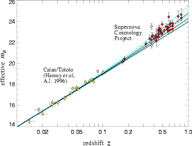
Figure 1.1: Diagramme de Hubble représentant le logarithme de $H_{{}_{0}}d_{\mathrm{L}}$ en fonction du redshift $z$. Ces données sont en faveur d’une accélération de l’expansion de l’univers [277].

La loi de Hubble (1.33) n’est cependant correcte que pour des objets proches pour lesquels la notion de distance n’est que peu affectée par la géométrie de l’univers. Ce n’est plus le cas pour des objets éloignés où différentes distances peuvent être définies en fonction des diverses observables comme le diamètre angulaire ou la luminosité apparente. Cette dernière permet de définir la distance luminosité $d_{\mathrm{L}}$ par

$$d_{\mathrm{L}}^{2}=\frac{{\mathcal{L}}}{4\pi{\mathcal{F}}},$$ (1.34)

${\mathcal{L}}$ étant la luminosité absolue, i.e. la puissance totale intrinsèque de la source, et ${\mathcal{F}}$ le flux mesuré, i.e. la puissance par unité de surface reçue. Dans le cas d’une métrique de type Minkowski, $d_{\mathrm{L}}$ est simplement la distance physique à la source, alors que dans le cadre du modèle FLRW, on s’attend à ce qu’elle dépende de l’expansion de l’univers. Intuitivement, pour une source située à la coordonnée comobile $r_{\mathrm{em}}$, la dilution de l’énergie par l’expansion introduit un facteur $(1+z)$ par dilatation des longueurs d’onde et un autre dû à la dilatation des temps d’émission (1.30). La surface actuelle de la sphère sur laquelle se dilue l’énergie émise par la source est, d’après (1.6), ${\mathcal{S}}=4\pi a^{2}_{{}_{0}}r_{\mathrm{em}}^{2}$. Le flux reçu est égal à ${\mathcal{F}}={\mathcal{L}}/\left[{\mathcal{S}}(1+z)^{2}\right]$ et on en déduit la distance luminosité

$$d_{\mathrm{L}}=a_{{}_{0}}r_{\mathrm{em}}(1+z).$$ (1.35)

La coordonnée comobile $r_{\mathrm{em}}$ de la source peut être exprimée en fonction des temps d’émission et de réception par (1.28). De plus, en développant le redshift (1.32) en $t_{\mathrm{em}}-t_{{}_{0}}$ pour des sources proches,

$$z\simeq H_{{}_{0}}(t_{{}_{0}}-t_{\mathrm{em}})+\left(1+\frac{q_{{}_{0}}}{2}\right)(t_{{}_{0}}-t_{\mathrm{em}})^{2},$$ (1.36)

et en inversant cette relation, la distance luminosité se développe en fonction du redshift

$$d_{\mathrm{L}}\simeq\frac{z}{H_{{}_{0}}}+\frac{1-q_{{}_{0}}}{2H_{{}_{0}}}z^{2}.$$ (1.37)

La quantité $q_{{}_{0}}=-\ddot{a}_{{}_{0}}a_{{}_{0}}/\dot{a_{{}_{0}}}^{2}$ est le paramètre de décélération, et s’exprime en fonction du paramètre de Hubble

$$q_{{}_{0}}=-\frac{{\mathcal{H}}_{{}_{0}}^{\prime}}{{\mathcal{H}}_{{}_{0}}^{2}}.$$ (1.38)

À l’aide de l’équation de Friedmann (1.16), avec $P_{{}_{0}}=0$ dans l’ère de matière, il vient

$$q_{{}_{0}}=\frac{\Omega_{{}_{0}}}{2}-\Omega_{\Lambda_{{}_{0}}}.$$ (1.39)

La relation (1.37) est la version “correcte” de la loi de Hubble (1.33), et au premier ordre en redshift, on retrouve la proportionnalité $z\simeq H_{0}d_{\mathrm{L}}$ (voir Fig. 1.1). Le paramètre de décélération quantifie donc les écarts à la loi de Hubble. Sa détermination est de plus un moyen de mesure des paramètres cosmologiques dont la densité d’énergie associée à la constante cosmologique [voir Eq. (1.39)].

La détermination de $d_{\mathrm{L}}$ comme une fonction du redshift a fait l’objet de multiples méthodes astrophysiques exploitant les propriétés intrinsèques des sources [225, 22, 133, 120, 94] (céphéïdes, relations masse-luminosité des galaxies, supernovae de type Ia …). La figure 1.1 représente des résultats relativement récents dans la détermination de $d_{\mathrm{L}}(z)$ par les courbes de luminosités des SNIa [277]. Les valeurs estimées des paramètres cosmologiques correspondants sont représentés sur la figure 1.2. La dégénérescence sur la détermination de la densité d’énergie associée à la matière peut être levée par l’utilisation d’autres données astrophysiques [263, 226, 323]. Ces résultats confirment de façon éclatante le modèle standard et semble indiquer, aujourd’hui, que la nature du fluide cosmologique fait intervenir une proportion importante de constante cosmologique

$$\Omega_{\Lambda_{{}_{0}}}\simeq 0.7,\qquad\Omega_{{}_{0}}\simeq 0.3,$$ (1.40)

indiquant que nous sommes actuellement dans une phase d’expansion accélérée d’un univers à faible courbure $\Omega_{\mathrm{tot}}\simeq 1$.

Figure 1.2: Détermination des paramètres de densité à partir de l’évolution de la distance luminosité pour les supernovae de type Ia. Dans le cadre du modèle standard, l’accélération de l’expansion de l’univers résulte de la prédominance actuelle de la constante cosmologique [277].

1.2.4 Histoire thermique

La conséquence majeure de l’expansion de l’univers est que le facteur d’échelle décroît lorsqu’on remonte dans le temps. Cette constatation implique, d’après les équations (1.20) et (1.32), que l’univers était plus dense et plus chaud par le passé, menant ainsi au concept de “big bang” chaud pour désigner l’instant initial où le facteur d’échelle pourrait s’annuler. La domination de la matière n’est donc certainement plus une hypothèse acceptable lorsqu’on remonte suffisamment loin dans le temps.

Si l’on considère, en effet, un fluide de radiation (ou de particules ultrarelativistes pour lesquelles la masse est négligeable devant l’impulsion), le terme de pression n’est plus négligeable

$$P_{\mathrm{rad}}=\frac{1}{3}\rho_{\mathrm{rad}},$$ (1.41)

et l’équation de conservation (1.18) donne une évolution de la densité d’énergie en

$$\rho_{\mathrm{rad}}\propto a^{-4}.$$ (1.42)

De manière générale, pour une équation d’état (1.19) avec $w$ constant, (1.18) s’intègre et la densité d’énergie varie en

$$\rho\propto a^{-3(1+w)}.$$ (1.43)

Il existe donc un instant $t_{\mathrm{eq}}$ où les densités d’énergie associé à la matière et au rayonnement étaient comparables, séparant l’ère de radiation pour $t<t_{\mathrm{eq}}$ où $\rho\simeq\rho_{\mathrm{rad}}$, de l’ère de matière où $\rho\simeq\rho_{\mathrm{mat}}$. Il est possible d’introduire une température associée à l’état thermodynamique du gaz de particule alors en interaction. Si l’on se place dans des conditions de pression telles que l’équilibre thermodynamique local soit vérifié, la densité d’énergie peut être obtenue à partir des statistiques de Fermi-Dirac ou de Bose-Einstein selon le spin des particules, et la température $\Theta$ définie au travers de la fonction de distribution dans l’espace des phases. Dans ce cas, la densité d’énergie est donnée par

$$\rho=\varsigma\int{{\mathrm{d}}^{3}\vec{p}\,\,Ef\left(\vec{p}\right)}=\varsigma\int{{\mathrm{d}}^{3}\vec{p}\,\,\delta_{\mathrm{e}}\frac{E}{{\mathrm{e}}^{(E-\chi)/\Theta}+\varepsilon}},$$ (1.44)

avec $E^{2}=p^{2}+m^{2}$ l’énergie totale de chaque particule, $\varsigma$ le facteur de dégénérescence associée à $\delta_{\mathrm{e}}=1/(2\pi)^{3}$ la densité d’état, $\chi$ le potentiel chimique, et $\varepsilon=\pm 1$ pour des fermions et bosons respectivement. Lors de l’ère dominée par la radiation, pour des particules ultra-relativistes telles que $E\simeq p$, en équilibre chimique, il vient

$$\rho_{\mathrm{B}}=\varsigma_{\mathrm{B}}\frac{\pi^{2}}{30}\Theta^{4}\qquad\rho_{\mathrm{F}}=\frac{7}{8}\varsigma_{\mathrm{F}}\frac{\pi^{2}}{30}\Theta^{4},$$ (1.45)

pour les bosons et les fermions respectivement. Ainsi, pour le fluide cosmologique constitué de matière baryonique usuelle et de rayonnement, la densité totale d’énergie est liée à la température par

$$\rho=\varsigma\frac{\pi^{2}}{30}\Theta^{4},$$ (1.46)

avec

$$\varsigma=\sum_{\mathrm{B}}\varsigma_{\mathrm{B}}+\frac{7}{8}\sum_{\mathrm{F}}\varsigma_{\mathrm{F}}.$$ (1.47)

La somme ne porte que sur les espèces effectivement relativistes à la température $\Theta$, et il est raisonnable de négliger l’énergie associée aux espèces non relativistes. Les équations (1.42) et (1.46) montrent que l’univers en expansion se refroidit comme on pouvait s’y attendre. Ainsi, au fur et à mesure du refroidissement de l’univers, les espèces vont de moins en moins interagir et vont finir par se découpler de l’équilibre thermodynamique, essentiellement lorsque leur libre parcours moyen $\Gamma^{-1}\simeq H^{-1}$, avec $H$ le paramètre de Hubble. Dépendant de la nature des espèces présentes, le facteur de dégénérescence va donc subir de brusques décroissances au cour de l’expansion jusqu’au dernier découplage, celui des photons.

Si l’on s’intéresse au devenir des espèces ultra-relativistes découplées de l’équilibre, la relation (1.46) n’est a priori plus valable, mais du fait de l’expansion, leur énergie est atténuée d’un facteur $a_{\mathrm{dec}}/a$ [voir Eq. (1.32)] pendant que la densité de particules $n$ décroît en $1/a^{3}$ par dilatation des longueurs. La fonction de distribution $f\left(\vec{p}\right)\propto{\mathrm{d}}^{3}n/{\mathrm{d}}\vec{p}^{\,3}$ reste donc invariante et égale à $f_{\mathrm{dec}}$. Ceci implique, d’après (1.44), que $E/\Theta$ est constant, soit

$$\Theta=\Theta_{\mathrm{dec}}\frac{a_{\mathrm{dec}}}{a}.$$ (1.48)

De la même manière, pour des espèces non relativistes, l’impulsion subissant toujours le redshift (1.32), la fonction de distribution reste invariante après découplage, et $E$ décroît d’un facteur $a^{2}$ menant à une variation de la température en $\Theta_{\mathrm{m}}\propto a^{-2}$. La conséquence fondamentale de ce scénario est l’existence actuelle d’un fond de rayonnement diffus de photons dans tout l’univers vérifiant une distribution de corps noir à la température (1.48). Ce fond de rayonnement d’origine cosmologique a été effectivement détecté par Penzias et Wilson [275], et vérifie une loi de corps noir à la température actuelle de $2.728\pm 0004\,{\mathrm{K}}$ (voir Fig. 1.3).

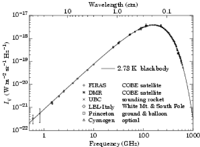
Figure 1.3: Le spectre du CMBR mesuré par différentes expériences [164].

L’origine physique du rayonnement fossile est dans le découplage entre la matière et les photons essentiellement dû à la recombinaison entre les électrons et les protons. Le redshift de la surface de dernière diffusion, i.e. le redshift à partir duquel l’univers est devenu transparent aux photons, peut ainsi être estimé par celui correspondant à la recombinaison, soit $z_{\mathrm{rec}}\simeq 1300$, et $\Theta_{\mathrm{rec}}\simeq 3500\,{\mathrm{K}}$ ou une énergie voisine de $0.3\,{\mathrm{eV}}$ [218].

L’histoire thermique de l’univers peut ainsi être comprise en s’approchant de la singularité initiale à partir de la connaissance de la microphysique dominante aux échelles d’énergie en question. À des échelles d’énergie de l’ordre de $\Theta\simeq 0.1-10\,{\mathrm{MeV}}$, les réactions nucléaires prennent place dans le plasma et sont à l’origine de la nucléosynthèse primordiale. Tester les conséquences de celle-ci revient à vérifier la validité du scénario du big bang chaud à l’époque la plus reculée qui nous soit actuellement accessible. En particulier, les abondances relatives des différents éléments produit par ces réactions nucléaires peuvent être calculées et sont en accord avec les observations (voir Fig. 1.4). Pour des températures de l’ordre de $\Theta\simeq 1\,{\mathrm{MeV}}$ le modèle standard prévoit également le découplage des neutrinos du plasma, leur température décroît alors en $a^{-1}$, comme les photons alors encore en équilibre thermique [cf. Eqs. (1.42) et (1.46)]. Cependant, le rayonnement de photons subit un réchauffement par annihilation électrons positrons. Il est possible de montrer que la conservation d’entropie génère sur le fluide de photons un accroissement de la température d’un facteur $(11/4)^{1/3}$. Puisque les neutrinos ne subissent pas cet effet c’est donc également le rapport de température entre les deux fluides après la recombinaison et il vient, pour l’époque actuelle, $\Theta_{\nu_{{}_{0}}}\simeq 1.95\,{\mathrm{K}}$.

Aux échelles d’énergie au delà de $100\,{\mathrm{MeV}}$, la description de l’univers nécessite l’emploi de la physique des hautes énergies que nous verrons dans le chapitre suivant. Quoiqu’il en soit, il existe une limite absolue au modèle standard qui est l’époque de Planck $\Theta_{\mathrm{Pl}}\simeq 10^{19}\,{\mathrm{GeV}}$ au delà de laquelle il est peu raisonnable de supposer que la relativité générale et les autres interactions ne constituent plus une description correcte de la Nature.

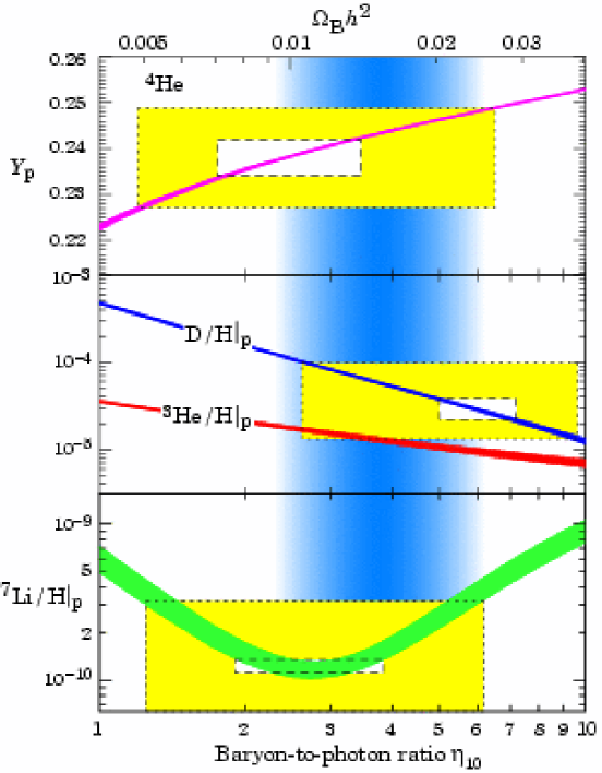
Figure 1.4: Prédiction à $95\%$ de confiance de l’abondance des éléments légers issus de la nucléosynthèse primordiale en fonction du rapport de la densité baryonique à la densité de rayonnement ($\eta_{10}$). Les diverses observables sont représentés par des boîtes rectangulaires et sont clairement en accord avec les prédictions [269, 164].

1.3 Les faiblesses du scénario standard

La validité du modèle standard de cosmologie ainsi brièvement décrit repose donc essentiellement sur l’observation du décalage vers le rouge des objets distants, de l’existence du fond diffus cosmologique et des abondances des éléments légers prédites par la nucléosynthèse primordiale. Bien qu’il soit possible de construire des théories alternatives pour chacune de ces observations séparément [43, 110, 188, 255], le modèle du big bang chaud reste le plus simple et complet pour décrire l’univers jusqu’à des énergies de l’ordre de la dizaine de$\,{\mathrm{MeV}}$.

Cependant, quelques observations ne trouvent pas d’explications raisonnables dans le cadre du modèle standard et doivent être décrites par l’intermédiaire de paramètres ad hoc. Comme nous le verrons dans le chapitre 3, elles ne peuvent être correctement interprétées que dans le cadre de l’univers primordial, à des échelles d’énergie bien au delà de la nucléosynthèse primordiale, nécessitant l’extrapolation de la physique des hautes énergies.

1.3.1 L’univers plat

Dans la section 1.2.3, nous avons vu que les valeurs mesurées des paramètres cosmologiques montrent que l’univers est actuellement de faible courbure $\Omega_{\mathrm{tot}}\simeq 1$ (cf. Fig. 1.2). Pour une équation d’état avec $w$ constant, à partir des équations (1.16) et (1.25), il vient

$$\Omega_{\mathrm{tot}}^{\prime}={\mathcal{H}}\left[(1+3w)\Omega-2\Omega_{\Lambda}\right]\left(\Omega_{\mathrm{tot}}-1\right).$$ (1.49)

La solution $\Omega_{\mathrm{tot}}=1$ est soit instable, soit un attracteur, selon le signe de $(1+3w)\Omega-2\Omega_{\Lambda}$. Dans un univers en expansion ${\mathcal{H}}>0$, et actuellement avec $w=0$ et $\Omega_{\Lambda_{{}_{0}}}\simeq 0.7$, $\Omega_{{}_{0}}\simeq 0.3$, cette solution est un attracteur. Cependant, il est facile de voir à partir des équations (1.21) à (1.24), (1.32) et (1.43) que

$$\frac{\Omega_{\Lambda}}{\Omega}=\frac{\Omega_{\Lambda_{{}_{0}}}}{\Omega_{{}_{0}}}\,(1+z)^{-3(1+w)},$$ (1.50)

et la domination du terme de constante cosmologique s’efface pour $z\simeq 0.7$. Il en résulte que pour des redshifts $z\gtrsim 1$, la platitude de l’univers est instable [334, 159]. Ceci reste valable dans l’ère de radiation avec $w=1/3$. Ainsi, pour que nous observions aujourd’hui $\Omega_{{\mathrm{tot}}_{{}_{0}}}\simeq 1$, il a fallu qu’au moment de l’équivalence, pour $z_{\mathrm{eq}}\simeq 10^{4}$, le paramètre de densité soit égal à l’unité à $10^{-3}$ près, et à $10^{-60}$ près à l’époque de Planck.

Un tel ajustement des conditions initiales nuit à la généricité du modèle et reflète certainement la présence d’autres phénomènes physiques dans l’univers primordial que nous évoquerons au chapitre 3.

1.3.2 L’homogénéité

L’hypothèse d’homogénéité de l’univers est contenue dans le principe cosmologique qui nous a permis d’écrire la métrique FLRW (1.6). Elle est donc à la base du modèle standard et confirmée par les observations. On peut néanmoins s’interroger sur les mécanismes physiques à l’origine de cette homogénéité. La fraction d’univers observable actuellement peut être quantifiée à partir de la métrique (1.6). Pour un observateur actuel situé au rayon comobile $r_{{}_{0}}=0$, les photons émis à $\eta_{\mathrm{em}}=0$, en la position $r_{\mathrm{H}}$ l’atteindront en un temps conforme $\eta$ tel que

$$\int_{\eta_{\mathrm{em}}}^{\eta}{\mathrm{d}}\eta^{\prime}=\pm\int_{r_{\mathrm{H}}}^{r_{{}_{0}}}\frac{{\mathrm{d}}r}{\sqrt{1-\mathsf{k}r^{2}}}.$$ (1.51)

Autrement dit, au temps conforme $\eta$, l’horizon des particules est précisément à la coordonnée comobile $r_{\mathrm{H}}$, les photons situés au delà de $r_{\mathrm{H}}$ n’ont donc pas encore, à $\eta$, atteint l’observateur. La distance propre à l’horizon est alors, d’après (1.6) et (1.51)

$$d_{\mathrm{H}}(\eta)=a(\eta)\int_{0}^{r_{\mathrm{H}}}\frac{{\mathrm{d}}r}{\sqrt{1-\mathsf{k}r^{2}}}=a(\eta)\eta,$$ (1.52)

ou, exprimée en fonction du temps cosmique

$$d_{\mathrm{H}}(t)=a(t)\int_{0}^{t}\frac{{\mathrm{d}}t^{\prime}}{a(t^{\prime})}.$$ (1.53)

Cette dernière équation montre plus clairement que la distance à l’horizon peut être infinie. Dans le cadre du modèle standard, pour $w$ constant et $w>-1$, l’équation de Friedmann (1.15) s’intègre à l’aide de (1.43) pour donner l’évolution du facteur d’échelle

$$a(t)\propto t^{\frac{2}{3(1+w)}} \Leftrightarrow a(\eta)\propto\eta^{\frac{2}{1+3w}}.$$ (1.54)

Si $w<-1/3$, l’équation (1.53) diverge en zéro et la distance à l’horizon est infinie. Inversement, pour $w>-1/3$, elle s’intègre et $d_{\mathrm{H}}$ est une fonction du temps

$$d_{\mathrm{H}}(t)\propto t \Leftrightarrow d_{\mathrm{H}}(\eta)\propto\eta^{\frac{3+3w}{1+3w}}.$$ (1.55)

Il en résulte que l’univers observable aujourd’hui contient des régions causalement disjointes du passé, la distance à l’horizon s’accroissant avec le temps cosmique. Ainsi, la distance propre actuelle à la surface de dernière diffusion est donnée par (1.51) et (1.52), avec $\eta_{\mathrm{em}}=\eta_{\mathrm{dec}}$, i.e.

$$d_{{\mathrm{dec}}}(\eta_{{}_{0}})=a_{{}_{0}}\left(\eta_{{}_{0}}-\eta_{\mathrm{dec}}\right).$$ (1.56)

et donc au moment du découplage, elle correspondait à une distance caractéristique de l’ordre de $d_{{\mathrm{dec}}}(\eta_{\mathrm{dec}})=(1+z_{\mathrm{dec}})^{-1}d_{{\mathrm{dec}}}(\eta_{{}_{0}})$. Il est possible de la comparer à la distance à l’horizon à cette époque, i.e. la distance propre au delà de laquelle les régions de l’univers à cette époque n’étaient plus causalement connectées. D’après (1.52), celle-ci se réduit à $d_{{\mathrm{H}}_{\mathrm{dec}}}=a_{\mathrm{dec}}\eta_{\mathrm{dec}}$. Le nombre de cellules projetées sur le ciel aujourd’hui et causalement déconnectés lors de la recombinaison est donc approximativement

$$n_{\mathrm{dec}}\simeq\left[\frac{d_{{\mathrm{dec}}}(\eta_{\mathrm{dec}})}{d_{{\mathrm{H}}_{\mathrm{dec}}}}\right]^{3}=\left(\frac{\eta_{{}_{0}}-\eta_{\mathrm{dec}}}{\eta_{\mathrm{dec}}}\right)^{3},$$ (1.57)

soit $n_{\mathrm{dec}}\simeq 10^{5}$ pour $z_{\mathrm{dec}}\simeq z_{\mathrm{rec}}\simeq 1300$. Inversement, la distance à l’horizon actuelle pour une cellule causale de la surface de dernière diffusion est $d_{{\mathrm{H}}_{\mathrm{dec}}}(\eta_{{}_{0}})=(1+z_{\mathrm{dec}})d_{{\mathrm{H}}_{\mathrm{dec}}}$, elle est donc actuellement vue sous un angle

$$\delta\theta\simeq\frac{d_{{\mathrm{H}}_{{\mathrm{dec}}}}(\eta_{{}_{0}})}{d_{{\mathrm{dec}}}(\eta_{{}_{0}})}=\frac{\eta_{\mathrm{dec}}}{\eta_{{}_{0}}-\eta_{\mathrm{dec}}}\simeq 0.8^{\circ}.$$ (1.58)

L’homogénéité entre ces régions causalement déconnectées lors de la recombinaison est observée aujourd’hui dans l’isotropie du spectre du CMBR (cf. Fig. 1.3) à $10^{-4}$ près. Le modèle standard ne permet pas de d’expliquer de telles corrélations entre ces différentes régions du ciel.

1.3.3 La formation des structures

La présence de structures gravitationnelles non linéaires aux petites échelles telles que les galaxies et les amas est interprétée comme le résultat de la croissance d’inhomogénéités de densité initiales par instabilité de Jeans (voir annexe 11.10). Dans le cadre du modèle de FLRW, en l’absence de constante cosmologique (voir Sect. 1.3.1), l’équation (1.49) s’intègre en fonction du facteur d’échelle

$$\frac{\Omega-1}{\Omega}\propto a^{1+3w},$$ (1.59)

qui peut se réécrire

$$\frac{\delta\Omega}{\Omega}\propto a^{1+3w},$$ (1.60)

avec $\delta\Omega=\Omega-1$ représentant l’écart du paramètre de densité à sa valeur critique dans un univers plat. Autrement dit, le contraste de densité dans un univers plat d’une région finie ayant une densité supérieure à la densité critique, i.e. $\Omega\gtrsim 1$, s’amplifie avec l’expansion de l’univers jusqu’à entrer dans le régime non-linéaire menant aux structures gravitationnelles observées. Dans le régime linéaire, il est toujours possible de développer le contraste de densité $\delta\rho/\rho$ en série de Fourier permettant de définir les longueurs d’onde $\lambda$ associées à ces fluctuations. Dans le modèle de FLRW, celles-ci sont dilatées par l’expansion, et les structures observées actuellement de longueur caractéristique $\lambda_{{}_{0}}$ correspondent à des fluctuations antérieures de longueur d’onde

$$\lambda=\frac{a}{a_{{}_{0}}}\lambda_{{}_{0}}.$$ (1.61)

À partir des équations (1.54) et (1.55), la distance à l’horizon évolue également avec le facteur d’échelle en

$$d_{\mathrm{H}}\propto a^{\frac{3(1+w)}{2}}.$$ (1.62)

En comparant (1.61) et (1.62), on voit donc qu’il existe un redshift pour lequel $\lambda>d_{\mathrm{H}}$ quelque soit $\lambda_{{}_{0}}$. Il est alors impossible dans le cadre du modèle de FLRW de trouver un mécanisme physique permettant de fixer de telles conditions initiales sur des distances correspondant à des régions causalement disjointes, ou superhorizons. Ce problème, comme celui de l’homogénéité, résulte directement de l’existence d’un horizon des particules et de la décélération de l’univers. Nous verrons dans le chapitre 3 qu’il est pleinement résolu par l’inflation.

1.4 Conclusion

Le modèle standard de la cosmologie fondé sur la gravitation d’Einstein est donc remarquablement confirmé par les observations pour des échelles d’énergie allant de $10^{-3}\,{\mathrm{eV}}$ aujourd’hui à quelques dizaines de$\,{\mathrm{MeV}}$ lors de la nucléosynthèse primordiale. Il attribue néanmoins des propriétés inexpliquées à notre univers, telle la platitude, l’accélération récente de l’expansion, une homogénéité “magique”… Ces problèmes laissent entrevoir l’existence d’autres phénomènes physiques à l’œuvre dans l’univers primordial. L’échelle de Planck, qui marque l’insuffisance supposée d’une description purement géométrique de l’espace-temps, se trouvant à des énergies de l’ordre de $10^{19}\,{\mathrm{GeV}}$, il est raisonnable d’espérer décrire ces phénomènes physiques, en deça de cette énergie, par la physique des hautes énergies couramment utilisée dans les expériences de physique des particules. Dans le prochain chapitre nous présenterons donc brièvement le modèle standard de la physique des particules, avant de nous intéresser à ses conséquences sur la cosmologie.

Chapitre 2 Le modèle standard de physique des particules

2.1 Introduction

Aux petites échelles de distances, par sa très faible intensité, la gravitation peut être négligée. Le monde microscopique sondé dans les accélérateurs de particules est ainsi régi par les trois autres interactions fondamentales de la Nature: l’électromagnétisme, l’interaction faible et l’interaction nucléaire forte. Le modèle standard de physique des particules donne un cadre théorique unifié décrivant l’interaction de la matière avec ces trois forces fondamentales. Pour cela, il s’appuie sur la théorie quantique des champs, issue de la relativité restreinte et de la mécanique quantique, où les objets fondamentaux sont des particules, événements de l’espace-temps, interagissant en respectant certaines symétries et dont les propriétés dépendent de l’échelle d’énergie à laquelle ils sont observés. Le modèle standard aujourd’hui comprend le modèle de Glashow, Weinberg et Salam [155, 355, 310] qui ont unifié l’électrodynamique quantique [136, 128, 312] et l’interaction faible en une théorie de jauge fondée sur la symétrie $SU(2)\times U(1)$, à l’aide du mécanisme de Higgs [131, 173, 165, 213]. Le mécanisme de Higgs est ainsi utilisé en physique des particules pour unifier les interactions et donner une explication à la masse des particules. Son existence est motivée par l’observation de ses conséquences, et les prédictions largement confirmées faites par ce modèle. Les généralisations de ce mécanisme sont intensément utilisées en cosmologie lors des transitions de phase, il est en outre à l’origine de la formation des cordes cosmiques par le mécanisme de Kibble [211]. L’interaction forte pouvant elle aussi être décrite par une théorie de jauge s’appuyant sur la symétrie $SU(3)$, la chromodynamique quantique, on parle alors de modèle standard $SU(3)\times SU(2)\times U(1)$.

2.2 Les théories de jauge

La représentation des invariances imposées par la relativité restreinte au travers du groupe de Poincaré se trouve réalisée en mécanique quantique par la différenciation des particules selon leur masse et leur spin. Ces symétries de base de l’espace-temps représentées dans l’espace de Hilbert de la mécanique quantique sont effectivement réalisées dans la Nature par les bosons, particules de spin entier, et les fermions de spin demi-entier. Les particules observées se réduisent ainsi aux scalaires $\Phi$ de spin nul, aux fermions $\Psi$ de spin $1/2$ et aux champs vectoriels $V^{\mu}$ de spin unité. En plus des symétries de base de l’espace-temps à l’origine des propriétés intrinsèques de la matière, la confirmation expérimentale du modèle standard suggère que les interactions entre ces particules sont elles aussi le produit de l’existence de symétries locales: les interactions sont en effet invariantes sous certaines transformations de coordonnées et des champs. Des charges peuvent être définies pour toutes les particules quantifiant leur comportement face à ces symétries locales, on construit alors une théorie, dite “de jauge”, quantifiée et prédictive [360, 367, 139, 361, 134].

2.2.1 L’électrodynamique

La théorie régissant les interactions électromagnétiques est basée sur la symétrie de jauge locale $U(1)$, i.e. l’invariance de l’interaction par la multiplication des champs par une phase complexe dépendant de l’événement. Cette symétrie est une des plus simple continue, car abélienne, permettant de construire une théorie de jauge et servira de modèle de prédilection pour l’étude des cordes cosmiques dans les chapitres suivants.

À l’aide du tenseur de Faraday $F^{\mu\nu}$, les équations de Maxwell [253] peuvent être réexprimées sous leur forme covariante

$$\partial_{\mu}F^{\mu\nu}=j^{\nu},\qquad\partial_{\mu}\widetilde{F}^{\mu\nu}=0,$$ (2.1)

avec

$$\widetilde{F}^{\mu\nu}=\frac{1}{2}\varepsilon^{\mu\nu\rho\sigma}F_{\rho\sigma},$$ (2.2)

le tenseur dual de $F$ dans l’espace de Minkowski, $j^{\mu}$ le quadrivecteur courant source du champ, et $\varepsilon^{\mu\nu\rho\sigma}$ le tenseur de Levi-Civita complètement antisymétrique dans ses indices et tel que $\varepsilon^{0123}=1$. Le tenseur $F^{\mu\nu}$ antisymétrique de rang $2$ vérifiant les identités de Bianchi

$$\partial_{\mu}F_{\nu\rho}+\partial_{\nu}F_{\rho\mu}+\partial_{\rho}F_{\mu\nu}\equiv\partial_{(\mu}F_{\nu\rho)}=0,$$ (2.3)

il s’exprime également comme un champ de gradient

$$F_{\mu\nu}=\partial_{\mu}A_{\nu}-\partial_{\nu}A_{\mu}\equiv\partial_{[\mu}A_{\nu]},$$ (2.4)

où $A^{\mu}$ est le potentiel vecteur associé. L’équation (2.4) est définie à un gradient près, c’est-à-dire qu’il existe une invariance de jauge des équations de Maxwell par rapport à n’importe quelle transformation du potentiel vecteur $A^{\mu}$ du type

$$A^{\mu}\rightarrow A^{\mu}-\partial^{\mu}{\mathcal{U}}(x^{\mu}),$$ (2.5)

où ${\mathcal{U}}(x^{\mu})$ est une fonction scalaire. L’évolution des champs électromagnétiques libres (2.1) peut également être obtenue par les équations d’Euler-Lagrange à partir de la densité lagrangienne

$${\mathcal{L}}_{\mathrm{em}}=-\frac{1}{4}F^{\mu\nu}F_{\mu\nu}-j_{\mu}A^{\mu}.$$ (2.6)

Si l’on s’intéresse maintenant aux fermions $\Psi(x^{\mu})$ de masse $m$, leur propagation libre est régie par le lagrangien de Dirac [115]

$${\mathcal{L}}_{\mathrm{f}}=\overline{\Psi}\left(i\gamma^{\mu}\partial_{\mu}-m\right)\Psi,$$ (2.7)

qui est trivialement invariant sous un changement de phase global $\Psi\rightarrow\Psi{\mathrm{e}}^{i\alpha}$. L’idée générale des théories de jauge est alors d’imposer une invariance locale, autrement dit on souhaiterait rendre le lagrangien de Dirac (2.7), indépendant des transformations $U(1)$ locales, i.e. $\Psi\rightarrow\Psi{\mathrm{e}}^{iq{\mathcal{U}}(x^{\mu})}$. Il est facile de voir, à partir de (2.7) que ceci n’est possible que par l’introduction d’un champ quadrivectoriel $A^{\mu}$ tel que

$$\Psi\rightarrow\Psi{\mathrm{e}}^{i{\mathcal{U}}(x^{\mu})}\quad\Rightarrow\quad A^{\mu}\rightarrow A^{\mu}-\partial^{\mu}{\mathcal{U}}(x^{\mu}),$$ (2.8)

à condition de remplacer le terme cinétique par une dérivée covariante sous ces transformations

$$D_{\mu}=\partial_{\mu}+iqA_{\mu}.$$ (2.9)

Le lagrangien des fermions invariant s’écrit alors

$${\mathcal{L}}_{\mathrm{f}}=\overline{\Psi}\left(i\gamma^{\mu}D_{\mu}-m\right)\Psi=\overline{\Psi}\left(i\gamma^{\mu}\partial_{\mu}-m\right)\Psi-q\overline{\Psi}\gamma^{\mu}\Psi A_{\mu}.$$ (2.10)

La dynamique propre du champ vectoriel $A_{\mu}$ vérifiant (2.8) ne peut être donnée que par les équations (2.1) et (2.4). Le dernier terme du lagrangien de Dirac invariant sous $U(1)$ s’interprète comme le terme source du champ électromagnétique avec $j^{\mu}=\overline{\Psi}\gamma^{\mu}\Psi$. Il est conservé car c’est également le courant de Nœther associé à l’invariance $U(1)$ de la théorie. Le champ bosonique $A^{\mu}$ auquel il est couplé [voir Eq. (2.10)] est la représentation de la particule médiatrice de l’interaction: le photon.

Ainsi, le simple fait d’imposer aux fermions libres l’invariance locale sous les transformations de jauge $U(1)$ permet de construire une théorie décrivant leurs interactions électromagnétiques par le biais d’un champ vectoriel qu’on interprète comme étant le photon. Le nouveau paramètre $q$ introduit est simplement la charge représentant la sensibilité des particules à ce nouveau couplage. Le lagrangien décrivant l’électrodynamique des fermions est donc

$${\mathcal{L}}_{{\mathrm{f}}{\mathrm{em}}}=-\frac{1}{4}F_{\mu\nu}F^{\mu\nu}+\overline{\Psi}\left(i\gamma^{\mu}D_{\mu}-m\right)\Psi.$$ (2.11)

De la même manière, à partir du lagrangien de Klein-Gordon [217] décrivant l’évolution libre des particules scalaires complexes,

$${\mathcal{L}}_{\mathrm{b}}=\frac{1}{2}\left(\partial_{\mu}\Phi\right)^{{\dagger}}\left(\partial^{\mu}\Phi\right)-\frac{1}{2}m^{2}\Phi^{\dagger}\Phi,$$ (2.12)

l’invariance par la symétrie de jauge locale $U(1)$ permet d’imposer leur couplage au champ électromagnétique. Le lagrangien de l’électrodynamique scalaire est alors donné par

$${\mathcal{L}}_{{\mathrm{b}}{\mathrm{em}}}=-\frac{1}{4}F_{\mu\nu}F^{\mu\nu}+\frac{1}{2}\left(D_{\mu}\Phi\right)^{{\dagger}}\left(D^{\mu}\Phi\right)-\frac{1}{2}m^{2}\Phi^{\dagger}\Phi.$$ (2.13)

La théorie $U(1)$ électromagnétique est aujourd’hui remarquablement vérifiée par l’expérience, ses prédictions sont en effet vérifiées à $10^{-13}$ près dans les accélérateurs [164].

2.2.2 La chromodynamique

L’interaction nucléaire forte, responsable de la cohésion des noyaux atomiques, peut également être décrite par une théorie de jauge fondée sur le groupe de symétrie non abélien $SU(3)$ rendant compte du confinement de cette interaction. Contrairement à l’électrodynamique, de portée infinie, cette dernière n’agit qu’aux échelles des nucléons, de l’ordre de $10^{-15}\,\mathrm{m}$.

Par analogie avec ce qui précède, on décrit l’interaction forte des quarks à partir du lagrangien de Dirac (2.7), en imposant son invariance sous les transformations du groupe $SU(3)$ des matrices ${\mathcal{U}}$ unitaires de rang $3$ et de déterminant unité, i.e. sous la transformation

$$\Psi^{i}\rightarrow{\mathcal{U}}^{i}_{j}\,\Psi^{j},$$ (2.14)

$\Psi^{i}$ étant cette fois un triplet de spineurs. Par soucis de simplicité, nous omettrons à partir d’ici ses indices. En suivant la même démarche que pour la symétrie $U(1)$, l’invariance locale est obtenue par l’introduction d’une matrice de champ vectoriel $\left(A^{\mu}\right)^{i}_{j}$ se transformant sous $SU(3)$ par

$$A^{\mu}\rightarrow{\mathcal{U}}A^{\mu}{\mathcal{U}}^{\dagger}-\frac{i}{g}\,{\mathcal{U}}\partial_{\mu}{\mathcal{U}}^{\dagger},$$ (2.15)

permettant de définir la matrice de dérivées covariantes

$$D_{\mu}=\partial_{\mu}+igA_{\mu}.$$ (2.16)

Par propriété de $SU(3)$, il y a huits champs vectoriels $A^{\mu}$ indépendants qui s’identifient aux générateurs du groupe et qui correspondent aux huit particules scalaires portant l’interaction et appelées les gluons. Leur dynamique propre peut également être obtenue par symétrie, en imposant l’invariance de jauge. La généralisation de (2.4) pour une symétrie non abélienne est

$${\mathcal{G}}_{\mu\nu}=\partial_{[\mu}A_{\nu]}+ig\left[A_{\mu},A_{\nu}\right],$$ (2.17)

et on montre que le lagrangien associé, invariant de Lorentz et conservant ls symétrie de parité, peut toujours se ramener à

$${\mathcal{L}}_{\mathrm{c}}=-\frac{1}{2}\mathrm{Tr}\left({\mathcal{G}}_{\mu\nu}{\mathcal{G}}^{\mu\nu}\right),$$ (2.18)

la trace portant sur les composantes matricielles [357]. La chromodynamique décrivant l’interaction des quarks et des gluons peut par conséquent être décrite par le lagrangien

$${\mathcal{L}}_{{\mathrm{q}}{\mathrm{c}}}=\sum_{{\mathrm{q}}}\overline{\Psi}_{\mathrm{q}}\left(i\gamma^{\mu}D_{\mu}-m_{\mathrm{q}}\right)\Psi_{\mathrm{q}}+{\mathcal{L}}_{\mathrm{c}}.$$ (2.19)

Il est alors possible de montrer que la charge portée par les quarks, appelée la couleur, est inobservable à nos échelles d’énergie dû aux propriétés de confinement de cette intéraction: son intensité est en effet d’autant plus forte que les échelles de distances observées sont grandes [91, 137, 41, 119, 372]. Les particules sensibles à l’intéraction forte, à nos échelles d’énergie, sont alors un assemblage de quarks et gluons de charge totale de couleur nulle, ou blanche, intéragissant par échange de mesons, des particules scalaires formés d’une paire quark-antiquark [148, 373, 164].

2.2.3 L’interaction électrofaible

La force faible est à l’origine des désintégrations $\beta^{\pm}$ violant la parité. La première théorie effective proposée était basée sur une interaction de type “courant-courant” [135, 325, 309] de lagrangien

$${\mathcal{L}}_{\mathrm{eff}}=-\frac{1}{\sqrt{2}}G_{\mathrm{f}}{\mathcal{J}}^{\mu}{\mathcal{J}}^{\dagger}_{\mu},$$ (2.20)

où les courants chargés ${\mathcal{J}}^{\mu}$ font intervenir les différents fermions couplés par l’interaction, i.e. les quarks $q$ et leptons $\ell$

$${\mathcal{J}}^{\mu}=\sum_{\ell}\overline{\Psi}_{\ell}\gamma^{\mu}\frac{1-\gamma^{5}}{2}\Psi_{\nu_{\ell}}+\sum_{q}\overline{\Psi}_{q}\gamma^{\mu}\frac{1-\gamma^{5}}{2}\Psi_{q^{\prime}}.$$ (2.21)

L’opérateur $\gamma^{5}$ introduit artificiellement, permet la violation de la parité observée dans les intéractions, et les couplages s’effectuent entre des doublets de particules générant une symétrie dite d’isospin faible. Ils sont formés d’un lepton et de son neutrino associé $(\ell,\nu_{\ell})$, et du doublet de quarks états propres de l’interaction $(q,q^{\prime})$. Cette théorie effective pose de nombreux problèmes, le plus important d’entre eux étant que la constante de couplage $G_{\mathrm{f}}$ est dimensionnée, rendant la théorie non renormalisable après quantification, i.e. non prédictive. Elle n’est pas une théorie de jauge et n’explique pas les interactions par courant neutre telles que les diffusions de neutrinos sur des électrons.

En constatant une symétrie globale d’isospin faible, on pourrait penser naturellement, suivant les exemples de l’électromagnétisme et des intéractions fortes, construire une théorie de jauge décrivant l’interaction faible se basant sur le groupe de Lie $SU(2)$. Comme pour la chromodynamique ou l’électrodynamique, une telle théorie introduirait des bosons vecteurs additionnels, au nombre de trois. La violation de la parité peut, quant à elle, être introduite au travers des représentations irréductibles de $SU(2)$, les particules de chiralité “droite” faisant partie d’un singulet de charge d’isospin nulle, et les particules “gauches”, sensibles à l’interaction, d’un doublet de charge $1/2$, comme suggéré par (2.21). En notant $\Psi_{\mathrm{L}}$ les doublets et $\Psi_{\mathrm{R}}$ les singulets, le lagrangien d’une telle théorie s’écrirait alors comme une somme sur les différentes familles de particules, les “saveurs”, des termes invariants de jauge

$${\mathcal{L}}_{\mathrm{w}}=\sum_{\mathrm{s}}\left[\,\overline{\Psi}^{\mathrm{s}}_{\mathrm{L}}\left(i\gamma^{\mu}D_{\mu}-m_{\mathrm{s}}\right)\Psi^{\mathrm{s}}_{\mathrm{L}}+\overline{\Psi}^{\mathrm{s}}_{\mathrm{R}}\left(i\gamma^{\mu}\partial_{\mu}-m_{\mathrm{s}}\right)\Psi^{\mathrm{s}}_{\mathrm{R}}\right]-\frac{1}{2}\mathrm{Tr}\left(W_{\mu\nu}W^{\mu\nu}\right),$$ (2.22)

où $W^{\mu}$ est la matrice de $SU(2)$ des bosons vecteurs, $W_{\mu\nu}$ son tenseur de type Faraday associé [cf. Eq. (2.17)] et la dérivée covariante pour les doublets

$$D_{\mu}=\partial_{\mu}+igW_{\mu},$$ (2.23)

$g$ étant la constante de couplage de l’interaction. En décomposant les bosons vecteurs $W^{\mu}$ sur les générateurs de $SU(2)$, i.e. les trois matrices de Pauli $\sigma^{i}$,

$$W=\sum_{i}W^{i}\frac{\sigma^{i}}{2},$$ (2.24)

il est possible de retrouver les courants chargés de la théorie effective, à ceci près que la constante de couplage $G_{\mathrm{f}}$ est maintenant remplacée par un terme faisant intervenir les propagateurs des bosons vectoriels chargés $W^{\pm}$ avec $W^{\pm}=(1/\sqrt{2})\left(W^{1}\pm W^{2}\right)$. De même, les intéractions de type courant neutre s’expliquent maintenant par l’échange du boson $W^{3}$.

Ces interactions ont d’autres parts la propriété de faire intervenir les charges électromagnétiques au sein même des bosons vecteurs $W^{\pm}$. Dans les interactions observées expérimentalement, on constate également la stricte conservation d’un nombre scalaire, l’hypercharge

$$Y=Q-T^{3},$$ (2.25)

où $Q$ est la charge électromagnétique et $T^{3}$ la projection d’isospin associée aux particules de $SU(2)$, i.e. $0$ pour les singulets et $\pm 1/2$ pour chaque composante des doublets, respectivement. Cette symétrie peut être jaugée par une symétrie locale $U(1)$ additionnelle unifiant l’électromagnétisme et les courants neutres [155]. Le lagrangien de la théorie s’écrit alors

$${\mathcal{L}}_{\mathrm{ew}}={\mathcal{L}}_{\mathrm{w}}-\frac{1}{4}B_{\mu\nu}B^{\mu\nu},$$ (2.26)

où les nouvelles dérivées covariantes apparaissant dans (2.22) pour les composantes gauches et droites, respectivement, sont données par

$$D_{\mu} = \partial_{\mu}+igW_{\mu}+ig^{\prime}Y^{\mathrm{s}}_{\mathrm{L}}B_{\mu},$$ (2.27)

$$D_{\mu} = \partial_{\mu}+ig^{\prime}Y^{\mathrm{s}}_{\mathrm{R}}B_{\mu}.$$ (2.28)

Une telle théorie ne décrit absolument pas les interactions qu’elle se propose de modéliser. En effet, les bosons vecteurs $W^{i}$ y sont prédits de masse nulle, suggérant une portée infinie de l’interaction faible, contrairement à ce qui est observé. Il faudrait en réalité qu’ils soient très massifs afin que l’influence de l’impulsion $k^{\mu}$ de ceux-ci soit négligeable devant leur masse pour que les termes en $gW^{i}$ dans le lagrangien donnent des propagateurs constants à basse énergie compatibles avec l’interaction “courant-courant”. Or des termes de masse en $m^{2}W^{\mu}W_{\mu}$ brisent l’invariance de jauge de la théorie. Le problème trouve sa solution dans le mécanisme de Higgs [131, 173, 165], qui introduit une particule scalaire supplémentaire à l’origine de la masse des particules auxquelles elle est couplée.

2.3 Le mécanisme de Higgs

Le mécanisme de Higgs [131, 173] met en jeu la brisure d’une symétrie, i.e. le non respect de la symétrie d’une théorie par l’état fondamental: l’idée en est simplement que si une équation admet une certaine symétrie et plusieurs solutions, celles-ci peuvent ne pas la respecter. Pour illustrer ce mécanisme, il est d’usage de considérer une symétrie $U(1)$ locale.

Soit le champ scalaire complexe $\Phi$ de Higgs, invariant sous les transformation de jauge $U(1)$, en auto-interaction dans un potentiel $V(\Phi)$. D’après (2.13), sa dynamique est régie par le lagrangien

$${\mathcal{L}}_{\mathrm{h}}=\frac{1}{2}\left(D_{\mu}\Phi\right)^{\dagger}\left(D^{\mu}\Phi\right)-\frac{1}{4}H_{\mu\nu}H^{\mu\nu}-V(\Phi),$$ (2.29)

où $H_{\mu\nu}$ est le tenseur de type Faraday associé au boson vectoriel $B_{\mu}$ tel que

$$D_{\mu}=\partial_{\mu}+igB_{\mu}.$$ (2.30)

La théorie est alors effectivement invariante sous les transformations de jauge

$$\Phi\rightarrow\Phi{\mathrm{e}}^{ig{\mathcal{U}}(x^{\mu})}\quad\textrm{et}\quad A^{\mu}\rightarrow A^{\mu}-\partial_{\mu}{\mathcal{U}}.$$ (2.31)

Pour pouvoir définir une théorie quantique renormalisable, et donc prédictive, le potentiel $V$ ne peut faire intervenir que des termes de masse et d’auto-interaction en $\Phi^{4}$, au plus. La brisure de symétrie intervient lorsque le potentiel $V$ est de la forme

$$V(\Phi)=\frac{\lambda}{8}\left(|\Phi|^{2}-\eta^{2}\right)^{2},$$ (2.32)

avec $\lambda$ la constante d’autocouplage du champ scalaire et $\eta$ sa valeur moyenne dans le vide. Dans ce cas, l’état fondamental stationnaire du champ est alors obtenu en imposant une énergie minimale, i.e. une valeur du potentiel minimale qui, d’après (2.32), est obtenue pour $|\Phi|^{2}=\eta$ (cf. Fig. 2.1).

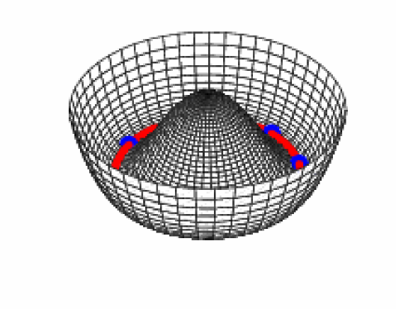
Figure 2.1: Le potentiel de Higgs $V(\Phi)$ tracé dans le plan complexe du champ scalaire $\left[\Re(\Phi),\Im(\Phi)\right]$. L’état d’énergie minimale est représenté en rouge et correspond à $|\Phi|=\eta$, différentes valeurs de phase apparaissent en bleu.

L’ensemble des valeurs moyennes du champ de Higgs dans son état fondamental est donc de la forme

$$\langle\Phi\rangle=\Phi_{{}_{0}}=\eta\,{\mathrm{e}}^{i\alpha},$$ (2.33)

avec $\alpha$ une phase complexe arbitraire (cf. Fig. 2.1). Chacun de ces états n’est clairement plus invariant sous les transformation de jauge $U(1)$, brisant ainsi la symétrie en question. Notons que le lagrangien à l’origine de la brisure et la théorie sous-jacente sont toujours invariants sous $U(1)$, ainsi que l’ensemble des états vides.

Pour explorer les conséquences physiques du phénomène il est commode de développer le champ de Higgs autour de son état fondamental afin d’en extraire la forme de ses excitations,

$$\Phi=\left[\eta+\rho(x^{\mu})\right]{\mathrm{e}}^{i\varphi(x^{\mu})/\eta}.$$ (2.34)

Pour de petites fluctuations autour de $\Phi_{{}_{0}}$, et en choisissant $\alpha=0$, ce qui localement est toujours possible, cette expression se réduit au premier ordre en

$$\Phi\simeq\eta+\rho+i\varphi,$$ (2.35)

dans la mesure où $\rho\ll\eta$ et $\varphi\ll\eta$. Le lagrangien (2.29) se développe alors, au deuxième ordre en ces champs, en

$${\mathcal{L}}_{\mathrm{h}} \rightarrow \frac{1}{2}\partial_{\mu}\rho\partial^{\mu}\rho+\frac{1}{2}\partial_{\mu}\varphi\partial^{\mu}\varphi-gB^{\mu}\left(\varphi\partial_{\mu}\rho-\rho\partial_{\mu}\varphi-\eta\partial_{\mu}\varphi\right)$$

$$+g^{2}\eta^{2}B_{\mu}B^{\mu}+g^{2}B_{\mu}B^{\mu}\left(\rho^{2}+\varphi^{2}+2\eta\rho\right)-\frac{\lambda}{2}\eta^{2}\rho^{2}.$$

La brisure de symétrie a donc donné naissance, a priori, à deux champs scalaires réels $\rho$ et $\varphi$. Le champ $\rho$ est un champ scalaire réel en interaction de masse $\sqrt{\lambda}\eta$, alors que le champ $\varphi$, quoiqu’également en intéraction, ne comporte pas de terme de masse [cf. Eq. (2.12)]; il est couramment appelé boson de Goldstone [157, 158, 260]. Physiquement les bosons de Goldstone ne peuvent exister que pour la brisure d’une symétrie globale, i.e. sans champ de jauge associé. En effet, dans le cas présent, le champ $\varphi$ peut être absorbé dans les transformations de jauge $U(1)$ de l’équation (2.31) en choisissant

$${\mathcal{U}}(x^{\mu})=-\frac{\varphi(x^{\mu})}{g\eta},$$ (2.37)

il ne constitue donc pas, pour une symétrie locale, un degré de liberté physique. Le résultat essentiel de ce mécanisme et que les bosons de jauge $B^{\mu}$ possèdent après brisure une masse physique $g\eta$ proportionnelle à la vev du champ de Higgs. Il est clair sur l’équation (2.29) que le lagrangien est effectivement invariant de jauge, et met en jeu maintenant, par le biais du champ de Higgs, des bosons vecteurs massifs.

Pour revenir à l’interaction électrofaible, le même mécanisme est généralisé à la symétrie $SU(2)\times U(1)$. La théorie décrivant cette interaction est effectivement celle résumée au paragraphe précédent, mais du fait du mécanisme de brisure de symétrie, seul la jauge $U(1)$ reste encore observable à basse énergie au travers de l’électrodynamique. Le mécanisme de Higgs appliqué à $SU(2)$ permet donc de donner une masse aux bosons vecteurs $W$, tout en conservant une théorie renormalisable [185, 186, 187]; il est par conséquent prédictif. En effet, considèrons un doublet de champs scalaires complexes d’hypercharge $Y_{\mathrm{h}}=1/2$

$$\Phi=\left(\begin{array}[]{c}\phi^{+}\\ \phi_{{}_{0}}\end{array}\right),$$ (2.38)

de lagrangien (2.29) dans lequel la dérivée covariante l’est maintenant par rapport aux transformations de $SU(2)\times U(1)$

$$D_{\mu}=\partial_{\mu}+igW_{\mu}+ig^{\prime}Y_{\mathrm{h}}B_{\mu}.$$ (2.39)

En choisissant la valeur moyenne dans le vide du doublet de Higgs le long de la composante non chargée

$$\langle\Phi\rangle=\left(\begin{array}[]{c}0\\ \eta\end{array}\right),$$ (2.40)

il est possible d’étudier, comme pour la brisure de $U(1)$, les fluctuations des champs dans leur nouvel état de vide en les décomposant sur les générateurs de $SU(2)$

$$\Phi=\left(\begin{array}[]{c}0\\ \eta+\rho\end{array}\right)\exp{\left(i\frac{\varphi_{j}}{\eta}\frac{\sigma^{j}}{2}\right)}.$$ (2.41)

Une transformation de jauge permet, comme dans le cas abélien, de réabsorber les phases $\varphi_{j}$ dans les masses, et de s’intéresser seulement au champ $\rho$. Le lagrangien se réduit donc, au deuxième ordre en ces nouveaux champs, à

$${\mathcal{L}}_{\mathrm{h}} \rightarrow \frac{1}{2}\partial_{\mu}\rho\partial^{\mu}\rho-\frac{\lambda}{2}\eta^{2}\rho^{2}+\frac{1}{2}g^{2}\eta^{2}W^{-}_{\mu}W^{\mu^{+}}+\frac{g^{2}}{2}\left(\rho^{2}+2\eta\rho\right)W^{-}_{\mu}W^{\mu^{+}}$$

$$+\left(\eta+\rho\right)^{2}\left[\left(g^{\prime}Y_{\mathrm{H}}B_{\mu}-\frac{g}{2}W_{\mu}^{3}\right)^{2}\right].$$

Comme pour la brisure de $U(1)$, il apparaît un champ scalaire neutre $\rho$ de masse $\sqrt{\lambda}\eta$, le boson de Higgs, et les bosons vecteurs $W^{\pm}$ acquièrent une masse $(1/2)g\eta$ comme $W^{3}$ et $B_{\mu}$ qui se trouvent maintenant couplés. Le couplage entre les bosons vecteurs neutres peut être mieux compris physiquement en introduisant deux nouveaux champs

$$Z_{\mu} = \cos(\theta_{\mathrm{w}})W_{\mu}^{3}-\sin(\theta_{\mathrm{w}})B_{\mu}$$ (2.43)

$$A_{\mu} = \sin(\theta_{\mathrm{w}})W_{\mu}^{3}+\cos(\theta_{\mathrm{w}})B_{\mu},$$ (2.44)

avec $\theta_{\mathrm{w}}$ l’angle faible défini par

$$\cos(\theta_{\mathrm{w}})=\frac{g}{\sqrt{g^{2}+g^{\prime 2}}}\qquad\sin(\theta_{\mathrm{w}})=\frac{g^{\prime}}{\sqrt{g^{2}+g^{\prime 2}}}.$$ (2.45)

Il est facile de voir à partir de (2.3) que les termes de masse et de couplage entre $W_{\mu}^{3}$ et $B_{\mu}$ se réduisent uniquement à un terme de couplage pour le boson $Z$ en

$${\mathcal{L}}_{\mathrm{Z}}=\frac{1}{4}(\eta+\rho)^{2}\left(g^{2}+g^{\prime 2}\right)Z_{\mu}Z^{\mu},$$ (2.46)

et que, autrement dit, le boson $A_{\mu}$ reste de masse nulle: il peut être identifié au photon générant la symétrie $U(1)$ électromagnétique, alors que le boson vecteur $Z_{\mu}$, à l’origine des courants neutre, est de masse $(1/2)\eta\sqrt{g^{2}+g^{\prime 2}}$. À partir du couplage entre neutrinos, de charge électromagnétique nulle, donné par (2.22), il est possible de relier les constantes de couplage introduites, i.e. $g$, $g^{\prime}$ et $\theta_{\mathrm{w}}$, à la constante de couplage électromagnétique $e$ par

$$e=g^{\prime}\cos(\theta_{\mathrm{w}})=g\sin(\theta_{\mathrm{w}}).$$ (2.47)

Expérimentalement, connaissant la constante de couplage effective de l’interaction faible $G_{\mathrm{f}}$, celle de l’électromagnétisme $e$, et l’angle faible $\theta_{\mathrm{w}}$ déterminé à partir des couplages $Z$ quarks et leptons [164], la masse des $W^{\pm}$ prédite est de $80.4\,{\mathrm{GeV}}$, et celle du $Z$, $91.6\,{\mathrm{GeV}}$. Ces particules ont effectivement été observées dans les accélérateurs avec des masses extrêmement voisines des valeurs prédites [164], confirmant ainsi le modèle de Glashow-Weinberg-Salam. Actuellement, la particule associé au Higgs $\rho$ aurait peut être été directement détectée (cf. Fig. 2.2), la mesure de sa masse fixerait alors la constante d’autocouplage $\lambda$ et confirmerait le mécanisme de Higgs.

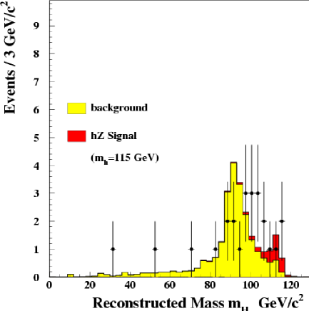
Figure 2.2: Distribution en masse du nombre d’évènements observés au LEP durant l’année 2000 et qui pourrait être interprétée comme une résonance du boson de Higgs à $115\,{\mathrm{GeV}}$ [93].

La masse des autres particules est obtenue par leur couplage au champ de Higgs. Ainsi pour des fermions, un couplage de type Yukawa [368] en

$$\lambda_{\mathrm{f}}\overline{\Psi}\Phi\Psi,$$ (2.48)

permet d’obtenir après brisure de symétrie des fermions $\Psi$ massifs de masse $\lambda_{\mathrm{f}}\eta$. Les différentes masses des diverses particules sont alors introduites par le biais de leur constante de couplage au champ de Higgs.

2.4 Prédictions et limites du modèle standard

Dans les sections précédentes, nous avons brièvement décrit les bases classiques du modèle standard. La théorie complète décrivant les interactions fondamentales nécessite cependant d’être quantifiée, donnant ainsi tout son sens à la notion de particule. Sans entrer dans le détail et les difficultés inhérentes à la quantification, celle-ci permet essentiellement de prédire les sections efficaces de toutes les interactions entre les particules, telles qu’on peut les mesurer dans les accélérateurs, mais également de les extrapoler à des échelles d’énergie bien plus élevées, telles celles de l’univers primordial.

2.4.1 La quantification et la renormalisation

L’existence physique d’une configuration de particules peut être identifiée, dans la théorie quantique des champs, à un état donné d’un espace de Fock, i.e. une supperposition infinie d’espaces de Hilbert dans lesquels évolue chaque particule. L’opérateur d’évolution $\widehat{U}(t_{i},t_{f})$ agissant dans cet espace permet de connaître l’amplitude de probabilité $S_{{\mathrm{i}}{\mathrm{f}}}$ de passage d’une configuration de particules $|{\mathcal{C}}_{\mathrm{i}}\rangle$ en $t_{\mathrm{i}}$, à la configuration finale $|{\mathcal{C}}_{\mathrm{f}}\rangle$ en $t_{\mathrm{f}}$. Il est possible de montrer que ces amplitudes de probabilités se réduisent aux calculs de la valeurs moyenne dans le vide initial du produit ordonné des champs en interaction [228, 313]

$$S_{{\mathrm{i}}{\mathrm{f}}}\propto\langle 0|\widehat{{\mathcal{T}}}\left[{\mathcal{F}}_{1}\dots{\mathcal{F}}_{n}\exp\left(i\int{{\mathrm{d}}^{4}{\mathbf{x}}}\,{\mathcal{L}}_{\mathrm{int}}\right)\right]|0\rangle,$$ (2.49)

où les ${\mathcal{F}}_{i}$ sont les champs considérés dans les états de Fock de transition et $\widehat{{\mathcal{T}}}$ l’opérateur produit ordonnant les champs selon les temps décroissants. Dans la représentation d’interaction, le terme ${\mathcal{L}}_{\mathrm{int}}$ se réduit aux parties du lagrangien de la théorie classique autre que celles décrivant la propagation libre des champs. Le membre de droite est aussi noté $G^{(n)}$ comme fonction de Green en interaction à $n$ points. Dans l’approche perturbative on développe l’opérateur d’évolution (le terme en exponentielle) en puissances successives de la constante de couplage et des champs libres. La fonction de Green de l’interaction se réduit en une somme infinie de termes faisant intervenir les fonctions de Green libres de la théorie à deux, trois, …, $n$ points qui s’identifient à

$$G^{(n)}_{\mathrm{lib}}=\langle 0|\widehat{{\mathcal{T}}}\left[{\mathcal{F}}_{1}\dots{\mathcal{F}}_{n}\right]|0\rangle$$ (2.50)

Celles-ci s’interprètent comme des corrections dues aux fluctuations quantiques des champs ${\mathcal{F}}$ en interactions, et sont souvent les seules qu’il est possible de calculer analytiquement.

Le calcul effectif des corrections quantiques peut s’effectuer au moyen de la quantification par l’intégrale de chemin [114, 138]. En effet, il est possible de montrer que la fonctionnelle

$$W\left[\left\{{\mathcal{J}}\right\}\right]\propto\int\left\{{\mathcal{D}}{\mathcal{F}}\right\}\exp\left[\int{{\mathrm{d}}^{4}{\mathbf{x}}}\left({\mathcal{L}}+{\mathcal{J}}{\mathcal{F}}\right)\right],$$ (2.51)

avec $\{{\mathcal{J}}\}$ l’ensemble des densités de courant externe, est génératrice des fonctions de Green en interaction

$$G^{(n)}=\frac{1}{i^{n}}\left.\frac{\delta^{n}W\left[\left\{{\mathcal{J}}\right\}\right]}{\delta{\mathcal{J}}^{n}}\right|_{\{{\mathcal{J}}\}=0}.$$ (2.52)

Il est ainsi possible de tenir compte des fluctuations quantiques des champs dans les interactions. Cependant, leur nature quantique ne s’accommode pas du tout de leur définition locale, et les termes apparaissant dans ce développement sont en général infinis. Pour rendre la théorie prédictive il faut alors procéder à la renormalisation.

Le processus de renormalisation consiste à ajouter un nombre fini de contre-termes, à un ordre donné, dans le lagrangien initial de manière à annuler ces divergences. Ces contre-termes peuvent alors être absorbés dans une redéfinition des champs et des constantes de la théorie, celles-ci devenant alors des fonctions de l’échelle d’énergie considérée. Les prédictions de la théorie sont finalement assurées par la connaissance de ces fonctions dont les variations avec l’énergie sont comparées et vérifiées par l’expérience (voir figure 2.3). C’est ’t Hooft [185, 186, 187] qui a montré que les théories de jauge avec brisure de symétrie étaient renormalisables sous certaines conditions fixant de manière unique la forme même des termes d’interaction à celles que nous avons utilisées dans les sections précédentes. Le modèle standard de la physique des particules ainsi construit décrit de manière satisfaisante la physique sondée dans les accélérateurs pour des énergies allant jusqu’à la centaine de $\,{\mathrm{GeV}}$. Il laisse néanmoins certaines questions en suspens dont les tentatives de réponse suggèrent que ce modèle ne constitue qu’une théorie effective d’une théorie physique plus complète.

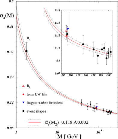
Figure 2.3: Évolution de la constante de couplage de l’interaction forte avec l’échelle d’énergie telle qu’elle est prédite par renormalisation, comparée aux valeurs mesurées [288]. Sa décroissance avec l’énergie est caractéristique de la liberté asymptotique de cette interaction.

2.4.2 L’unification

La forme unifiée de l’interaction électrofaible du modèle standard pose naturellement le problème de l’unification des autres interactions. Pourquoi deux interactions seulement seraient la manifestation d’un même phénomène ? Par la renormalisation des constantes de couplage, il est possible d’en calculer leur évolution avec l’échelle d’énergie (cf. Fig. 2.3), et les mesures actuelles semblent montrer que ces constantes sont du même ordre de grandeur lorsque les énergies échangées sont de l’ordre de $10^{15}\,{\mathrm{GeV}}$ (cf. Fig. 2.4), suggérant que la chromodynamique devait également être unifiée avec l’interaction électrofaible [149, 89].

Un problème d’envergure réside également dans l’inclusion de la gravitation. Celle-ci peut également être exprimée sous forme d’une théorie de jauge sous les transformations locales de coordonnées dont l’action s’écrit [175]

$${\mathcal{S}}_{\mathrm{g}}=\int{\frac{1}{2\kappa^{2}}\left(R-2\Lambda\right)\sqrt{-g}\,{\mathrm{d}}^{4}{\mathbf{x}}},$$ (2.53)

où $R$ est le scalaire de Ricci et $g$ le déterminant de la métrique. La constante de couplage $\kappa^{2}$ étant dimensionnée, la gravitation d’Einstein n’est pas renormalisable, et donc non prédictive après quantification. Du point de vue théorique, ceci renforce l’idée selon laquelle le modèle standard incluant la gravité cette fois-ci, n’est qu’une théorie effective à basse énergie. Néanmoins, l’échelle d’énergie à laquelle les effets quantiques sont susceptibles de modifier notablement la gravité est celle de Planck, i.e. $10^{19}\,{\mathrm{GeV}}$ et donc dans la pratique, largement au delà des échelles d’unification des autres interactions. La relativité générale est encore, à ces énergies, une très bonne description de la gravitation.

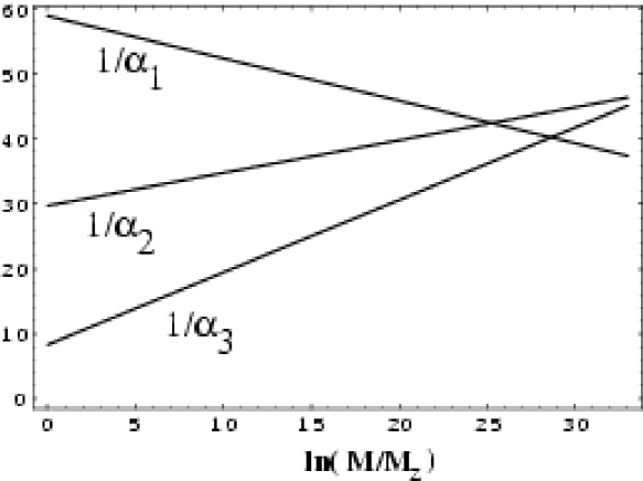
Figure 2.4: Évolution des constantes de couplage des trois interactions fondamentales avec l’échelle d’énergie. $\alpha_{1}$ est la constante associée à la symétrie d’hypercharge, i.e. $\alpha_{1}=(5/3)\alpha_{\mathrm{e}}/\cos^{2}(\theta_{\mathrm{w}})$ et $\alpha_{2}$ celle associée à $SU(2)$, i.e. $\alpha_{2}=\alpha_{\mathrm{e}}/\sin^{2}(\theta_{\mathrm{w}})$ où $\alpha_{\mathrm{e}}={\mathrm{e}}^{2}/(4\pi)$. $\alpha_{3}$ est la constante de couplage de l’interaction forte. Elles semblent s’unifier autour de $10^{15}\,{\mathrm{GeV}}$ [239].

2.4.3 Les paramètres libres

Bien que vérifié au pourcent près, le modèle standard met en jeu $19$ paramètres indépendants qui sont les constantes de couplage, les angles de mélange et les masses (ou constantes de couplage au Higgs) des diverses particules, ce qui n’est pas complètement satisfaisant du point de vue théorique.

Le modèle standard ne propose aucune explication relative à la quantification de la charge, i.e. au fait que les charges des quarks sont en $e/3$ exactement, $e$ étant la charge de l’électron. Cette symétrie entre leptons et hadrons suggère également que ces paramètres a priori indépendants pourraient être reliés dans une théorie plus générale.

Le modèle standard ne donne pas non plus d’explication au problème de hiérarchie des masses. La brisure de symétrie électrofaible donne une échelle d’énergie naturelle à la théorie autour de $\eta\simeq 175\,{\mathrm{GeV}}$. Bien que le quark top possède une masse de cet ordre, les autres particules s’étalent sur un spectre de masse bien plus large, ainsi, pour décrire des électrons de masse $511\,{\mathrm{KeV}}$, il faut que leur constante de couplage soit extraordinairement faible, ce qui est encore une forme de fine tunning.

Enfin, la renormalisation de la théorie introduit un nouveau paramètre $M$ qui est l’échelle d’énergie considérée, et dont dépendent les autres paramètres du modèle. Pour un champ scalaire, à l’ordre d’une boucle, il est possible de montrer que les contre-termes ajoutés au lagrangien initial (nu) renormalisent sa masse en

$$m^{2}_{{}_{0}}\rightarrow m^{2}=m^{2}_{{}_{0}}+{\mathcal{O}}(M^{2}).$$ (2.54)

La masse physique observée est $m$ alors que $m_{{}_{0}}$ est le paramètre fondamental de la théorie. Si la théorie dont on mesure les effets aujourd’hui est valable jusqu’à l’échelle de Planck, i.e. $M\simeq 10^{19}\,{\mathrm{GeV}}$, alors pour observer un boson de Higgs de $115\,{\mathrm{GeV}}$ il faudrait que $m_{{}_{0}}/M$ soit ajusté à $10^{-17}$ près dans la théorie fondamentale.

2.4.4 L’énergie du vide

Le vide tel qu’il est interprété en théorie quantique des champs est sujet aux fluctuations quantiques des multiples champs en interactions. Bien que de valeurs moyennes nulles, celles-ci contribuent néanmoins à l’énergie du vide telle qu’elle apparaît dans la constante cosmologique des équations de Friedmann (1.15) si on suppose que les théories de physique des particules sont couplées à la gravitation, ne serait-ce que par les termes cinétiques. Ainsi pour un champ scalaire libre de lagrangien (2.12), la densité d’énergie du champ dans l’état de vide s’obtient à partir du tenseur énergie-impulsion

$$\langle 0|T_{tt}|0\rangle=\langle 0|\frac{1}{2}\left[\sum_{\mu}\left(\partial_{\mu}\Phi\right)^{2}+m^{2}\Phi^{2}\right]|0\rangle.$$ (2.55)

Avec ${\mathbf{p}}$ le quadrivecteur impulsion du champ et après quantification du champ scalaire, il vient

$$\langle 0|T_{tt}|0\rangle=\int{\frac{{\mathrm{d}}^{3}\vec{p}}{(2\pi)^{3}2p^{0}}}\,\left(|\vec{p}\,|^{2}+m^{2}\right).$$ (2.56)

Dans le cas particulier d’un champ de masse nulle, et en intégrant jusqu’à l’énergie de Planck, toujours en supposant que le modèle standard y est encore valable, l’équation (2.56) se simplifie en

$$\langle 0|T_{tt}|0\rangle\simeq\frac{1}{16\pi^{2}}M_{\mathrm{Pl}}^{4}.$$ (2.57)

La densité critique actuelle est de l’ordre de $10^{-29}{\mathrm{g}}/{\mathrm{cm}}^{3}$, soit dans les unités favorites $1\,{\mathrm{meV}}^{4}$. La contribution d’un tel champ à l’énergie du vide serait donc de l’ordre de $\Omega_{\mathrm{vac}}\simeq 10^{124}$, à comparer à la valeur actuelle $\Omega_{\Lambda_{{}_{0}}}\simeq 0.7$ mesurée par l’expansion de l’univers. Ce terme ne pose pas de problème s’il n’y a pas de couplage gravitationnel (${\mathcal{G}}=0$) car il peut être renormalisé à zéro, mais ce n’est plus le cas lorsque la gravité est considérée.

2.5 Conclusion

Le modèle standard de physique des particules est une excellente description des interactions électrofaible et nucléaire forte au moins jusqu’à des énergies de l’ordre de quelques centaines de $\,{\mathrm{GeV}}$. Ses prédictions vérifiées au pourcent près constituent une base solide des mécanismes qu’il invoque, tel que la brisure de symétrie par le biais d’un champ de Higgs. La découverte de sa particule associée en sera certainement la meilleure confirmation. Néanmoins, il laisse ouvert de nombreuses questions montrant qu’il n’est que la partie visible à nos échelles d’une théorie plus fondamentale. Le problème est que l’énergie potentiellement accessible dans des accélérateurs humains n’atteindra jamais, dans un futur prévisible, les échelles où la physique semble être radicalement différente. Cependant, comme nous l’avons évoqué au chapitre 1, ces énergies ont déjà été atteintes dans l’histoire de l’univers du fait de l’expansion. Ainsi, l’étude de l’univers primordial à des échelles d’énergies supérieures à $10^{3}\,{\mathrm{GeV}}$, i.e. un univers âgé de moins de $10^{-11}{\mathrm{s}}$, permet de sonder les théories de physique des particules alors à l’œuvre. Inversement, la description quantique des champs est certainement celle qu’il convient d’utiliser dans l’univers primordial. La symbiose existant entre ces deux branches de la physique est effectivement fructueuse, et, comme nous le verrons dans les chapitres suivants, permet de donner des éléments de réponse aux faiblesses des deux modèles standards, mais également de poser de nouvelles questions.

Chapitre 3 Au delà des modèles standards

3.1 Introduction

Les modèles standard de cosmologie et de physique des particules décrivant correctement la physique “à basse énergie”, les quelques extensions évoquées dans cette section vont donc concerner l’univers primordial, i.e des énergies supérieures à l’échelle de brisure électrofaible où l’univers était âgé de moins de $10^{-11}{\mathrm{s}}$. Le rôle essentiel du champ de Higgs dans cette transition de phase est certainement un exemple de l’importance qu’ont pu avoir les champs scalaires à ces époques. Ainsi, à l’approche hydrodynamique usuelle décrivant le contenu matériel de l’univers, est souvent préférée l’approche théorie des champs en espace-temps courbe. La dynamique de l’univers primordial est alors régie par les lois d’évolution d’un ou plusieurs champs quantiques.

3.2 Les champs scalaires cosmologiques

3.2.1 L’inflation

L’idée qu’un champ scalaire ait pu dominer la dynamique de l’univers primordial est à l’origine du mécanisme d’inflation, i.e. une phase d’accélération de l’expansion de l’univers, qui s’avère résoudre les problèmes du modèle de FLRW liés à l’existence d’un horizon des particules [166]. L’idée générale est que l’observation actuelle de régions causalement déconnectées du passé résulte de l’accroissement plus rapide de la distance à l’horizon par rapport au facteur d’échelle, ce qui est directement la conséquence du ralentissement de l’expansion dans l’ère de radiation et de matière. Le plus simple de ces modèles invoque le lagrangien (2.12) d’un champ scalaire $\Phi$ dans un potentiel $V(\Phi)$ en espace-temps courbe

$${\mathcal{L}}_{\mathrm{inf}}=\frac{1}{2}g_{\mu\nu}\partial^{\mu}\Phi\partial^{\nu}\Phi-V(\Phi),$$ (3.1)

dont l’évolution s’obtient à partir de l’équation de Klein-Gordon

$$\frac{1}{\sqrt{-g}}\,\partial_{\mu}\left(\sqrt{-g}g^{\mu\nu}\partial_{\nu}\Phi\right)+\frac{{\mathrm{d}}V}{{\mathrm{d}}\Phi}=0,$$ (3.2)

avec $g$ le déterminant de la métrique. Pour une métrique de FLRW (1.6) et un champ scalaire homogène, il vient

$$\ddot{\Phi}+3H\dot{\Phi}+\frac{{\mathrm{d}}V}{{\mathrm{d}}\Phi}=0.$$ (3.3)

La densité d’énergie et la pression associées à ce champ peuvent s’obtenir à partir de son tenseur énergie-impulsion

$$T_{\mu\nu}=\frac{2}{\sqrt{-g}}\frac{\delta\left(\sqrt{-g}{\mathcal{L}}\right)}{\delta g^{\mu\nu}}=2\frac{\delta{\mathcal{L}}}{\delta g^{\mu\nu}}-g_{\mu\nu}{\mathcal{L}}.$$ (3.4)

Par identification de (3.4) avec le tenseur énergie-impulsion (1.10) d’un fluide parfait, l’équation (3.1) donne

$$\rho_{\phi} = \frac{1}{2}\dot{\Phi}^{2}+V(\Phi),$$ (3.5)

$$P_{\phi} = \frac{1}{2}\dot{\Phi}^{2}-V(\Phi).$$ (3.6)

La dynamique de l’univers est donnée par les équations de Friedmann (1.15) et (1.16) qui deviennent

$$H^{2} = \frac{\kappa^{2}}{3}\left[\frac{1}{2}\dot{\Phi}+V(\Phi)\right],$$ (3.7)

$$\dot{H} = -\frac{\kappa^{2}}{2}\dot{\Phi}^{2},$$ (3.8)

où les termes de courbure et de constante cosmologique ont été négligés puisque l’on s’intéresse à l’univers primordial (cf. Sect. 1.3.1). Dans le régime dit de “roulement lent” où l’énergie cinétique du champ scalaire reste négligeable devant son énergie potentielle, i.e.

$$\frac{1}{2}\dot{\Phi}^{2}\ll V(\Phi)\quad\textrm{et}\quad\ddot{\Phi}\ll 3H\dot{\Phi},$$ (3.9)

il vient

$$\rho_{\phi}\simeq-P_{\phi}\simeq V(\Phi),$$ (3.10)

et la dynamique de l’univers s’apparente alors à celle conduite par un terme de constante cosmologique pure $P_{\Lambda}=-\rho_{\Lambda}$ [voir Eq. (1.24)]. Les équations de Friedmann (3.7) et (3.8) se simplifient en

$$H^{2}\simeq\frac{\kappa^{2}}{3}V(\Phi),\qquad|\dot{H}|\ll H^{2},$$ (3.11)

et l’expansion de l’univers est accélérée garantissant la phase d’inflation

$${\mathcal{H}}^{\prime}=a\ddot{a}=a^{2}\left(\dot{H}+H^{2}\right)>0.$$ (3.12)

À partir des Eqs. (3.3) et (3.9), les potentiels satisfaisant les conditions de roulement lent doivent vérifier

$$\left|\frac{1}{V}\frac{{\mathrm{d}}V}{{\mathrm{d}}\Phi}\right|^{2}\ll 6\kappa^{2}.$$ (3.13)

La présence d’une telle période inflationnaire permet de résoudre le problème de l’horizon. Au premier ordre, d’après (3.11), le paramètre de Hubble est constant donnant lieu à une croissance exponentielle du facteur d’échelle

$$a\propto{\mathrm{e}}^{Ht}.$$ (3.14)

Pendant cette période, la distance à l’horizon des particules (1.53) se réduit à

$$d_{{\mathrm{H}}_{\mathrm{inf}}}=\frac{1}{H}{\mathrm{e}}^{Ht}\left(1-{\mathrm{e}}^{-Ht}\right)\simeq\frac{1}{H}{\mathrm{e}}^{Ht},$$ (3.15)

pourvu que $Ht$ soit suffisamment grand, ce qui sera vérifié a posteriori. Ainsi, le rapport des distances à l’horizon entre le début d’une phase inflationnaire à $t_{\mathrm{i}}$ et sa fin à $t_{\mathrm{f}}$ vaut

$$\frac{d_{{\mathrm{H}}}(t_{\mathrm{f}})}{d_{{\mathrm{H}}}(t_{\mathrm{i}})}={\mathrm{e}}^{H\Delta t},$$ (3.16)

avec $\Delta t=t_{\mathrm{f}}-t_{\mathrm{i}}$. La distance à l’horizon au temps de Planck est d’après (1.52) $d_{{\mathrm{H}}_{\mathrm{Pl}}}=a_{\mathrm{Pl}}\,\eta_{\mathrm{Pl}}$, alors que la distance propre actuelle au mur de Planck est $d_{{\mathrm{Pl}}}(\eta_{{}_{0}})=a_{{}_{0}}\,(\eta_{{}_{0}}-\eta_{\mathrm{Pl}})$, qui ramenée au temps de Planck devient $d_{{\mathrm{Pl}}}(\eta_{\mathrm{Pl}})=a_{\mathrm{Pl}}\,(\eta_{{}_{0}}-\eta_{\mathrm{Pl}})$. Comme pour la surface de dernière diffusion, cette dernière est de plusieurs ordres de grandeur plus grande que l’horizon à cette époque. Le problème de l’horizon est donc résolu par l’inflation si

$$d_{{\mathrm{H}}_{{\mathrm{Pl}}_{\mathrm{inf}}}}={\mathrm{e}}^{H\Delta t}d_{{\mathrm{H}}_{\mathrm{Pl}}}>d_{{\mathrm{Pl}}}(\eta_{\mathrm{Pl}}),$$ (3.17)

ou encore pour une phase inflationnaire telle que

$${\mathrm{e}}^{H\Delta t}>\frac{\eta_{{}_{0}}-\eta_{\mathrm{Pl}}}{\eta_{\mathrm{Pl}}}\simeq 10^{29}.$$ (3.18)

Un tel facteur d’expansion est obtenue pour $H\Delta t\simeq 67$ et vérifie donc l’hypothèse (3.15). Physiquement, la phase inflationnaire gonfle rapidement une région causale au temps de Planck de sorte qu’elle englobe aujourd’hui tout l’univers observable.

L’inflation résout aussi naturellement le problème de la platitude, en effet l’équation (1.49) d’évolution du paramètre de densité devient

$$\dot{\Omega}_{\mathrm{tot}}=-2H\Omega_{\mathrm{tot}}\left(\Omega_{\mathrm{tot}}-1\right),$$ (3.19)

qui s’intègre en

$$\frac{\Omega_{{\mathrm{tot}}}(t_{\mathrm{f}})-1}{\Omega_{{\mathrm{tot}}}(t_{\mathrm{f}})}=\frac{\Omega_{{\mathrm{tot}}}(t_{\mathrm{i}})-1}{\Omega_{{\mathrm{tot}}}(t_{\mathrm{i}})}{\mathrm{e}}^{-2H\Delta t}.$$ (3.20)

Ainsi, pour un taux d’expansion de $H\Delta t\simeq 67$, le paramètre de densité se retrouve $10^{60}$ fois plus proche de l’unité qu’il ne l’était avant la phase d’inflation, ce qui compense l’instabilité de $\Omega_{\mathrm{tot}}=1$ par l’évolution ultérieure du facteur d’échelle (cf. chapitre 1.3.1).

Enfin, l’inflation résout également le problème de la formation des grandes structures. Comme présenté dans la section 1.3.3, les équations (1.61) et (1.62) montrent que les longueurs d’onde $\lambda_{{}_{0}}$ caractéristiques des structures gravitationnelles actuellement observées se retrouvent toujours, dans le modèle standard, en dehors de l’horizon initialement, ce qui pose le problème de leur origine physique. Par l’inflation, la distance à l’horizon étant exponentiellement dilatée selon (3.15), les fluctuations originelles de longueur d’onde $\lambda$, donnée par (1.61), se retrouvent initialement à des échelles subhorizons [218]. L’inflation autorise ainsi l’existence de mécanismes physiques causals leurs donnant naissance.

Bien que très attrayant, le mécanisme d’inflation laisse indéterminé la nature du champ scalaire dominant la dynamique, “l’inflaton”. De nombreux modèles ont été développés permettant de le resituer dans un cadre plus large [284, 233, 220, 232]. En particulier, les transitions de phase peuvent être utilisées pour lui donner naissance [166, 167, 234], la brisure de symétrie permettant de changer la configuration du champ de Higgs de $\Phi=0$ à $\Phi=\eta$ (voir chap. 2), et sous certaines conditions d’obtenir un régime de roulement lent. Ces modèles permettent alors de prévoir le devenir de l’inflaton lorsque celui-ci atteint son nouvel état d’équilibre, afin de mieux contraindre les classes de modèles admissibles [10, 1, 117, 218].

3.2.2 La quintessence

Comme cela a été évoqué au chapitre 2, le modèle standard de physique des particules prévoit une contribution gigantesque des champs quantiques à l’énergie du vide qui n’est absolument pas observé en cosmologie. Ce problème [354] est le résultat de l’impossibilité de redéfinir arbitrairement le vide lorsque l’on considère la gravité, et dont la cause peut être vue comme due à notre ignorance de la théorie quantique de la gravitation. Si elle existe, les équations d’Einstein (1.13) peuvent en effet se réécrire sous la forme

$$G_{\mu\nu}=\kappa^{2}T_{\mu\nu}-\Lambda_{\mathrm{nue}}\,g_{\mu\nu}.$$ (3.21)

Il est clair que, comme on l’a fait dans la section 2.4.4, considérer une valeur moyenne dans le vide pour l’opérateur tenseur énergie-impulsion $\langle 0|T_{\mu\nu}|0\rangle$, revient à bien définir la valeur moyenne de l’opérateur $G_{\mu\nu}$, ce que l’on ne sait actuellement pas faire. Néanmoins, il est toujours possible de considérer que les champs classiques bosoniques en jeu dans les deux membres de (3.21) représentent la valeur moyenne des excitations de ces hypothétiques champs quantiques bien définis d’une théorie plus vaste, et l’on a ici noté $\Lambda_{\mathrm{nue}}$ le terme de constante cosmologique ainsi obtenu. Il est raisonnable d’imaginer qu’une symétrie de cette théorie puisse induire une compensation exacte telle que

$$\kappa^{2}\langle 0|T_{\mu\nu}|0\rangle=\Lambda_{\mathrm{nue}}g_{\mu\nu},$$ (3.22)

annulant ainsi le terme d’énergie du vide (2.57) dans la dynamique cosmologique [363]. L’échelle naturelle de $\Lambda_{\mathrm{nue}}$ serait alors de l’ordre la masse de Planck, ce qui semble compatible avec le domaine de prédominance de la gravité quantique.

Le problème est alors d’expliquer pourquoi la constante cosmologique effective actuellement observée ($\Omega_{\Lambda_{{}_{0}}}\simeq 0.7$) n’est pas rigoureusement nulle, sans introduire un fine tunning entre les deux termes de l’équation (3.22) puisqu’alors la différence entre les deux termes serait ajustée à $10^{-124}$ près. Les modèles de quintessence proposent que l’effet observé actuellement soit dû à un autre champ scalaire cosmologique induisant une accélération de l’univers, la compensation dans (3.22) étant par ailleurs supposée exacte [351, 359].

Un tel champ scalaire peut également être décrit par (3.1) avec cette fois un potentiel de la forme [274, 294]

$$V(\Phi)=\frac{M^{4+\alpha}}{\Phi^{\alpha}},$$ (3.23)

où $M$ et $\alpha$ sont des paramètres libres. De tels potentiels permettent l’existence d’un attracteur pour l’évolution cosmologique du champ scalaire. Il est possible de montrer [37] que indépendamment des conditions initiales, la densité d’énergie du champ de quintessence (3.5) évolue en

$$\rho_{\phi}\propto a^{-\frac{3\alpha(1+w)}{2+\alpha}}.$$ (3.24)

Elle décroît plus lentement que celle associée à la matière et la radiation pourvu que $\alpha>0$ [voir Eq. (1.43)], et donc il existe un moment, après la phase dominée par la matière, où l’énergie du champ va dominer l’univers, et d’après les équations (3.10), agir comme un terme de constante cosmologique dans l’approximation du roulement lent. Une fois fixé $\rho_{\phi_{{}_{0}}}$ tel que $\Omega_{\phi_{{}_{0}}}\simeq 0.7$, la prédominance uniquement récente du champ scalaire sur la matière est également vérifiée, comme c’était le cas pour une constante cosmologique pure [voir Eq. (1.50)]. D’autres parts l’insensibilité aux conditions initiales est assurée par le fait qu’il existe un attracteur, et fixe les paramètres du modèle à des échelles d’énergie raisonnables, $M\simeq 10^{6}\,{\mathrm{GeV}}$ lorsque $\alpha=6$ par exemple, rendant le modèle acceptable du point de vue de la physique des hautes énergies.

La quintessence résout donc le deuxième problème de fine tunning de la constante cosmologique, elle est de plus prédictive puisque la domination actuelle du champ scalaire en question donne une équation d’état différente de celle d’une constante cosmologique pure. D’après les équations (3.5) et (3.6), lorsque le champ entre dans le régime de roulement lent

$$w_{\phi}=\frac{P_{\phi}}{\rho_{\phi}}\simeq-1+\frac{\dot{\Phi}^{2}}{V(\Phi)}>-1.$$ (3.25)

La mesure du paramètre $w$, prévue dans les années à venir, de l’équation d’état du fluide cosmologique qui domine maintenant, permettra de tester les modèles de quintessence [160].

Comme dans le cas de l’inflation, l’origine du champ de quintessence est indéterminée. Il est possible de montrer que le potentiel (3.23) mène à une valeur physique du champ actuelle $\Phi\simeq M_{\mathrm{Pl}}$ suggérant un lien avec des théories quantiques de gravité. L’existence physique de ces champs scalaires cosmologiques est également motivée par les extensions du modèles standard de physique des particules, et principalement par la supersymétrie.

3.2.3 La supersymétrie

Les représentations du groupe de Poincaré sont réalisées dans la Nature par les fermions et des bosons. Cependant, le modèle standard de physique des particules $SU(3)\times SU(2)\times U(1)$ introduit une dissymétrie entre ces deux familles: les fermions constituent essentiellement la matière alors que les bosons n’apparaissent que comme vecteurs de leurs interactions. La supersymétrie introduit une nouvelle symétrie entre fermions et bosons, qui de ce fait doit s’insérer dans le groupe de Poincaré. Il est possible de montrer qu’une telle symétrie est unique, et ne peut être générée que par des opérateurs $Q_{r}$ de type fermionique vérifiant les relations d’anticommutations [358, 311]

$$\left\{Q_{r},\overline{Q}_{s}\right\} = 2\gamma^{\mu}_{rs}P_{\mu},$$ (3.26)

$$\left[Q_{r},P^{\mu}\right] = 0,$$ (3.27)

$$\left[Q_{r},M^{\mu\nu}\right] = i\,\sigma^{\mu\nu}_{rs}Q_{s},$$ (3.28)

où les $Q_{s}$ sont des opérateurs de spin $1/2$ sous les transformations de Lorentz de chiralité choisie, autrement dit des spineurs de Majorana. Le choix de l’anticommutateur est imposé par le théorème de Coleman-Mandula [92] et les autres relations de commutations sont fixées par les conditions de covariance et de fermeture de l’algèbre ainsi générée. $\sigma^{\mu\nu}$ est le générateur des transformations de Lorentz $M^{\mu\nu}$ dans la représentation de spin $1/2$

$$\sigma^{\mu\nu}=\frac{1}{4}\left[\gamma^{\mu},\gamma^{\nu}\right].$$ (3.29)

La réalisation d’une telle symétrie impose qu’à tout fermion $|{\mathrm{f}}\rangle$ soit associé un boson de même masse $|{\mathrm{b}}\rangle$. La relation de commutation (3.27) donne en effet

$$m^{2}_{\mathrm{b}}|{\mathrm{b}}\rangle=P^{\mu}P_{\mu}Q_{s}|{\mathrm{f}}\rangle=Q_{s}P^{\mu}P_{\mu}|{\mathrm{f}}\rangle=m_{\mathrm{f}}^{2}|{\mathrm{b}}\rangle.$$ (3.30)

Le fermion et son boson associé peuvent être vus comme des partenaires supersymétriques d’un même objet, un supermultiplet. Dans le cas d’un champ scalaire et d’un spineur, on parle de supermultiplet chiral dont le lagrangien le plus simple doit être invariant sous les transformations globales de supersymétrie $\delta_{\xi}$: les générateurs $Q$ étant spinoriels, il en est de même pour les paramètres infinitésimaux $\xi$ de ces transformations. Le supermultiplet chiral se transforme en [24]

$$\delta_{\xi}\Psi = i\gamma^{\mu}\partial_{\mu}\left(A+i\gamma^{5}B\right)\xi$$ (3.31)

$$\delta_{\xi}A = \overline{\xi}\Psi$$ (3.32)

$$\delta_{\xi}B = i\overline{\xi}\gamma^{5}\Psi,$$ (3.33)

où les champs $A$ et $B$ sont les parties réelles et imaginaires du champ scalaire complexe $\Phi$. On peut alors vérifier que le lagrangien de Wess-Zumino [358]

$${\mathcal{L}}_{\mathrm{wz}}=\partial_{\mu}\Phi^{\dagger}\partial^{\mu}\Phi+i\overline{\Psi}\gamma^{\mu}\partial_{\mu}\Psi,$$ (3.34)

est effectivement invariant sous les transformations (3.31) à (3.33), sur couche de masse, i.e. lorsque les champs vérifient leurs équations du mouvement. Une telle symétrie n’est pas observée à nos échelles d’énergie. Par conséquent, si elle existe, elle a nécessairement été brisée dans l’univers primordial. L’existence de la supersymétrie est néanmoins suggérée par certaines de ses conséquences.

La symétrie fermions bosons générée par la supersymétrie résout le problème des corrections radiatives évoquées au chapitre 2. Le développement perturbatif de la fonctionnelle génératrice des fonctions de Green (2.51) comprend alors autant de termes invoquant des fermions que des bosons, leur contribution étant de signe opposée, les divergences éventuelles tendent ainsi à se compenser. Les théories supersymétriques sont donc plus facilement renormalisables, quand elles ne sont pas simplement finies. Ces compensations ont également la particularité d’annuler l’énergie du vide quantique (2.56). Bien sûr, la brisure de supersymétrie restaure ce problème, mais à une échelle d’énergie très inférieure à celle de Planck.

Une autre prédiction attrayante de l’existence de la supersymétrie concerne les théories d’unification des interactions [268]. Dans la section 2.4.2, on a vu que la variation des constantes de couplage avec l’échelle d’énergie tend à indiquer leur unification autour de $10^{15}\,{\mathrm{GeV}}$. Les théories de grande unification essaient de trouver des groupes de jauge redonnant ceux du modèle standard après brisure d’une symétrie plus vaste [comme $SU(5)$ ou $SO(10)$] par le mécanisme de Higgs. L’adjonction de la supersymétrie dans ces théories donne une meilleure unification des constantes de couplages suggérant sa restauration à haute énergie (cf. Figs. 2.4 et 3.1).

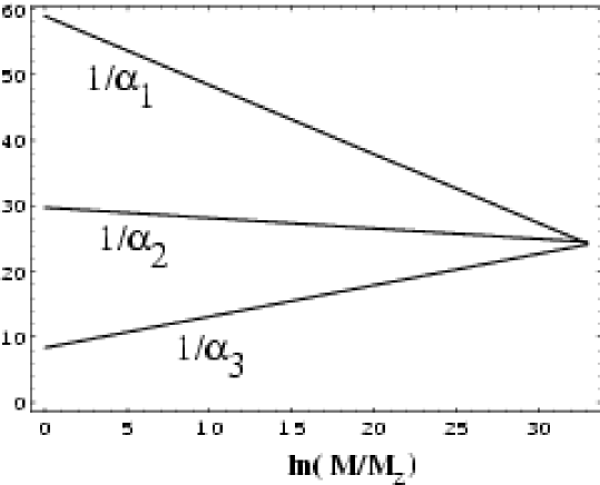
Figure 3.1: Évolution des constantes de couplage des trois interactions fondamentales avec l’échelle d’énergie, dans le cadre des théories de grande unification supersymétriques [239]. Les paramètres $\alpha_{i}$ sont les constantes de couplage associées aux trois interactions tels qu’ils sont définis sur la figure 2.4.

Enfin il est possible de construire une théorie invariante sous les transformations locales de supersymétrie. Les relations de commutations (3.26) à (3.28) mettant en jeu les générateurs du groupe de Poincaré, l’invariance sous les transformations locales de coordonnées sera donc naturellement assurée, d’où sa dénomination de supergravité. À partir du lagrangien de Wess-Zumino (3.34), il est possible de montrer [24, 141, 267] que la théorie correspondante invariante sous $\delta_{\xi({\mathbf{x}})}$ introduit alors la relativité générale ainsi qu’un fermion de spin $3/2$ interprété comme le partenaire supersymétrique du graviton.

$$\delta_{\xi({\mathbf{x}})}{\mathcal{L}}_{\mathrm{wz}}=0\Rightarrow{\mathcal{L}}_{\mathrm{wz}}=\partial_{\mu}\Phi^{\dagger}\partial^{\mu}\Phi+i\overline{\Psi}\gamma^{\mu}\partial_{\mu}\Psi+\frac{1}{2\kappa^{2}}R+\frac{1}{2}\varepsilon^{\mu\nu\rho\sigma}\overline{\Psi}_{\mu}\gamma^{5}\gamma_{\nu}\partial_{\rho}\Psi_{\sigma},$$ (3.35)

avec $R$ le scalaire de Ricci, et $\Psi^{\mu}$ le champ fermionique de spin $3/2$ décrit par l’action de Rarita-Schwinger [293]. La supergravité, en plus de donner un cadre unifié à toutes les interactions, offre des mécanismes de brisure de supersymétrie dans des secteurs cachés, i.e. pour des champs couplés aux particules usuelles uniquement par la gravitation. Ces brisures douces aboutissent à une séparation de la masse des scalaires et fermions à basse énergie compatible avec l’absence d’observations [99, 268, 26], et potentiellement détectable. Par exemple, pour une échelle d’énergie de brisure de supersymétrie de l’ordre de $10^{10}\,{\mathrm{GeV}}$, le gravitino aurait une masse de $100\,{\mathrm{GeV}}$ [24]. Du point de vue cosmologique, les potentiels de supergravité permettent de donner un cadre plus rigoureux à la quintessence. Il est en effet possible de montrer que les potentiels en exponentielle

$$V(\Phi)\propto{\mathrm{e}}^{-\alpha\Phi},$$ (3.36)

naturellement présents en supergravité, mènent à des solutions attractives compatibles avec les observations [55, 56], tout en résolvant le problème des corrections dues à la gravitation (cf. Sect. 3.2.2).

La supersymétrie donne donc un cadre théorique motivant l’existence de champs scalaires dans l’univers primordial. De plus toutes ces théories mettent en jeu des mécanismes de brisure de symétrie, faisant également intervenir d’autres champs scalaires, permettant de retrouver le comportement du modèle standard à basse énergie. La physique des particules actuelle donne donc la vision d’un univers primordial à la dynamique régie par l’évolution d’un ou plusieurs de ces champs et ponctuée de brisures de symétrie. Cependant, les brisures spontanées de symétrie ne sont pas sans conséquences du point de vue cosmologique. T. Kibble a en effet montré dans les années 1970 [210, 211] qu’elles pouvaient conduire à l’apparition de défauts topologiques du vide, c’est à dire des régions de l’espace dans lesquelles les champs restent piégés dans leur ancien état de vide. L’énergie contenue dans ces objets dépendant explicitement de l’échelle d’énergie de la brisure de symétrie, et pouvant être assez élevée, leur existence peut effectivement modifier les propriétés de l’univers.

3.3 Les défauts topologiques

La transition de phase survenant lors de la brisure de symétrie par mécanisme de Higgs (cf. Sect. 2.3) s’insère dans le cadre cosmologique lorsque l’on considère les effets de la température. Aux échelles d’énergie du modèle standard, l’état fondamental permettant de définir la fonctionnelle génératrice des fonctions de Green (2.51) est le vide à température nulle (cf. Sect. 2.4.1). Cette approximation n’est cependant plus valable dans l’univers primordial puisque les interactions entre les divers champs s’effectuent dans un bain thermique de température $\Theta$ non nulle, et les fonctions de Green libres (2.50) doivent être redéfinies sur un ensemble complet d’états $|\Omega\rangle$ qui sont supposés appartenir à l’ensemble grand canonique:

$$G^{(n)}_{\Theta}\propto\sum_{\Omega}{\mathrm{e}}^{-\beta E_{\Omega}}\langle\Omega|\widehat{{\mathcal{T}}}\left[{\mathcal{F}}_{1}\dots{\mathcal{F}}_{n}\right]|\Omega\rangle,$$ (3.37)

où $\beta=1/\Theta$. Il est possible de montrer que le formalisme de renormalisation, utilisé à température nulle pour calculer les corrections radiatives, s’applique également au calcul des corrections due au bain thermique [251, 244, 4, 53] pourvu que la variable temporelle soit bornée sur l’intervalle $[0,-i\beta]$.

Ainsi, dans le cadre du modèle de Higgs abélien, il est possible de tenir compte des corrections au potentiel du champ scalaire (2.32) à la température $\Theta$. Le potentiel effectif à une boucle s’écrit alors [353, 116, 214]

$$V_{\mathrm{eff}}\left(\Phi,\Theta\right)=\frac{\lambda}{8}|\Phi|^{4}+\frac{\lambda}{24}\left(\Theta^{2}-6\eta^{2}\right)|\Phi|^{2}+\eta^{4}.$$ (3.38)

Pour des températures

$$\Theta>\Theta_{\mathrm{c}}=\sqrt{6}\eta,$$ (3.39)

ce potentiel ne possède qu’un minimum à $|\Phi|=0$. Lorsque la température devient inférieure à cette valeur critique, on se retrouve dans une situation de brisure spontanée de symétrie où l’état fondamental devient dégénéré $|\Phi|=\eta$ (voir Fig. 2.1). Inversement, les symétries brisées des modèles de physique des particules sont donc restaurées dans l’univers primordial pourvu que la température y soit suffisamment élevée. En conséquence, lors de son refroidissement, l’univers est le siège de multiples transitions de phase où l’état d’énergie du vide change de manière plus ou moins rapide selon la nature de la transition.

Toujours pour le modèle de Higgs abélien, lorsque la température de l’univers passe en dessous de $\Theta_{\mathrm{c}}$, le champ “tombe” en chaque point de l’espace physique dans son nouvel état de valeur moyenne

$$\Phi_{{}_{0}}=\eta\,{\mathrm{e}}^{i\alpha}.$$ (3.40)

La phase complexe étant a priori quelconque, sur des distances physiques plus grandes que la longueur de corrélation $\ell_{\mathrm{c}}$ de la transition de phase, celle-ci va être une fonction continue de la position $\alpha\left(\vec{x}\right)$. L’existence d’une longueur de corrélation est assurée par l’existence d’une distance finie à l’horizon à cette époque. En pratique, un ordre de grandeur de $\ell_{\mathrm{c}}$ est plutôt donné par la microphysique à l’œuvre lors de la transition et peut être relié à l’échelle de distance des fluctuations thermiques [210]. Une fois les phases déterminées par la transition, on peut chercher un contour fermé le long duquel $\alpha\left(\vec{x}\right)$ varie continûment de $0$ à un multiple entier de $2\pi$. Si une telle configuration existe, cela implique nécessairement, par continuité, l’existence d’un point à l’intérieur de cette boucle où la phase $\alpha$ ne peut être correctement définie. Le seul état du champ de Higgs autorisant cette phase singulière est $\Phi_{{}_{0}}=0$, soit l’état de vide avant la transition. Par translation dans les dimensions transverses à la boucle, il se forme donc une structure linéique où le champ de Higgs est nul et appelée corde de Kibble ou corde cosmique (voir Fig. 3.2). Plus intuitivement, l’ensemble des choix de phases possibles en chaque point de l’espace survenant lors de la transition va générer des configurations telles qu’en certains points singuliers l’ancien vide ne peut choisir son nouvel état, et une fois les fluctuations de température suffisamment faibles pour ne plus modifier la configuration des phases, cet état se retrouve gelé en une corde cosmique.

Figure 3.2: Le potentiel de Higgs du modèle $U(1)$ abélien dans le plan complexe $\left[\Re\left(\Phi\right),\Im\left(\Phi\right)\right]$ et la topologie des phases du nouvel état de vide, dans l’espace physique, menant à la formation d’une corde cosmique.

3.3.1 Cordes de Nielsen-Olesen

À partir du lagrangien du modèle de Higgs abélien (2.29), des solutions de type cordes cosmiques peuvent être trouvées en se restreignant à des solutions statiques à symétrie cylindrique, et il est toujours possible d’écrire localement les champs de Higgs et de jauge sous la forme [3, 264]

$$\Phi=\varphi(r){\mathrm{e}}^{in\theta},\qquad B_{\mu}=B_{\theta}(r)\delta_{\mu\theta},$$ (3.41)

avec $\varphi$ et $B_{\theta}$ des champs scalaires réels dans le plan polaire $(r,\theta)$. Les équations du mouvement vérifiées par le champ de Higgs et le champ de jauge se simplifient alors en

$$\frac{{\mathrm{d}}^{2}H}{{\mathrm{d}}\varrho^{2}}+\frac{1}{\varrho}\frac{{\mathrm{d}}H}{{\mathrm{d}}\varrho} = \frac{HQ^{2}}{\varrho^{2}}+\frac{1}{2}H(H^{2}-1),$$ (3.42)

$$\frac{{\mathrm{d}}^{2}Q}{{\mathrm{d}}\varrho^{2}}-\frac{1}{\varrho}\ \frac{{\mathrm{d}}Q}{{\mathrm{d}}\varrho} = \frac{m_{\mathrm{b}}^{2}}{m_{\mathrm{h}}^{2}}H^{2}Q,$$ (3.43)

avec $m_{\mathrm{b}}=g\eta$ et $m_{\mathrm{h}}=\sqrt{\lambda}\eta$ les masses du boson vectoriel et du boson de Higgs, et les variables adimensionnées

$$H=\frac{\varphi}{\eta},\quad Q=n+gB_{\theta}\quad\textrm{et}\quad\varrho=m_{\mathrm{h}}r.$$ (3.44)

La solution de ces équations est représentée sur la figure 3.3 pour un nombre d’enroulement $n=1$. Le champ de Higgs s’annule au centre du vortex pour rejoindre sa valeur moyenne $\eta$ dans le vide loin de la corde, alors que le champ vectoriel se condense sur la corde où la symétrie n’est pas brisée [6, 23, 282, 303]. La largeur physique de la corde est donnée par l’échelle de distance sur laquelle varie le champ de Higgs, et celle-ci est de l’ordre de sa longueur d’onde Compton (cf. Fig 3.3)

$$\varnothing_{\mathrm{c}}\simeq 1/m_{\mathrm{h}}.$$ (3.45)

Figure 3.3: Les solutions de cordes statiques, à symétrie cylindrique, aux équations de champs déduites du lagrangien de Higgs abélien (2.29). Le champ de Higgs $H$ s’annule au centre du vortex et rejoint son état de vide usuel sur des distances de l’ordre de $1/m_{\mathrm{h}}$, alors que les bosons de jauge se condensent sur la corde.

L’énergie contenue dans cette configuration de corde peut être explicitement calculée à partir de ces solutions de champs et des équations (2.29) et (3.4). Par symétrie cylindrique, seules les composantes temporelles et axiales sont non nulles après intégration sur les variables transverses [279], il vient alors

$$T^{tt}=-T^{zz}=-{\mathcal{L}}_{\mathrm{h}}=\frac{1}{2}\left(\partial_{r}\varphi\right)^{2}+\frac{1}{2}\frac{\varphi^{2}Q^{2}}{r^{2}}+V(\varphi)+\frac{1}{2g^{2}}\frac{\left(\partial_{r}Q\right)^{2}}{r^{2}},$$ (3.46)

soit, en fonction des variables adimensionnées

$$T^{tt}=\frac{\lambda\eta^{4}}{2}\left[\left(\partial_{\varrho}H\right)^{2}+\frac{Q^{2}H^{2}}{\varrho^{2}}+\frac{(H^{2}-1)^{2}}{4}+\frac{1}{\lambda g^{2}}\frac{\left(\partial_{\varrho}Q\right)^{2}}{\varrho^{2}}\right].$$ (3.47)

L’énergie par unité de longueur $U$ s’obtient ensuite par intégration sur les variables transverses

$$U=C\!\left(\lambda g^{2}\right)\,\eta^{2},$$ (3.48)

avec $C$ une fonction des constantes de couplage de l’ordre de l’unité [341]. La densité d’énergie d’une corde cosmique est donc directement donnée par l’échelle d’énergie de la brisure de symétrie. Ainsi, des cordes de grande unification formées à $10^{15}\,{\mathrm{GeV}}$ ont une masse linéique voisine de $10^{15}$ tonnes par cm et un diamètre $10^{-22}$ fois plus petit que celui de l’atome d’hydrogène. Pour des échelles d’énergie autour de $10\,{\mathrm{TeV}}$, la densité d’énergie est proche du gramme par centimètre pour des rayons dix million de fois plus petits que l’atome d’hydrogène. Dans la vision hydrodynamique, par analogie avec (1.10), $-T^{zz}$ représente la tension de la corde $T$. D’après l’équation (3.46) les cordes cosmiques basées sur le modèle de Higgs abélien vérifient donc

$$U=T\simeq\eta^{2}.$$ (3.49)

La brisure de la symétrie $U(1)$ par le mécanisme de Higgs donne ainsi naissance à des défauts dans la configuration spatiale du vide. Comme évoqué au paragraphe précédent, la stabilité de ces objets est intimement liée à la topologie du vide après la transition de phase. D’une manière plus générale, il est possible d’utiliser une approche mathématique basée sur les groupes d’homotopie du vide pour statuer sur leur nature et existence après une brisure de symétrie.

3.3.2 Topologie du vide

De manière générale, lors d’une transition de phase par brisure de symétrie, l’état d’énergie minimale passe d’une invariance sous les transformations d’un groupe de Lie compact $G$, à un sous groupe $H$. La brisure de symétrie est généralement notée $G\rightarrow H$. Avec les notations utilisées dans la section précédente, l’état de vide brisant la symétrie est défini par

$$\Phi_{{}_{0}}=\langle 0|\Phi|0\rangle,$$ (3.50)

et le sous groupe non brisé

$$H\equiv\left\{h\in G{\,\diagup\,}{\mathcal{R}}(h)\Phi_{{}_{0}}=\Phi_{{}_{0}}\right\},$$ (3.51)

où ${\mathcal{R}}(h)$ sont les matrices de la représentation du groupe de symétrie $G$ dans l’espace vectoriel où évolue le champ $\Phi$. Le vide obtenu peut alors être représenté par une variété ${\mathcal{V}}$ définie par

$${\mathcal{V}}\equiv\left\{\Phi_{\mathrm{v}}{\,\diagup\,}\Phi_{\mathrm{v}}={\mathcal{R}}(v)\Phi_{{}_{0}};v\in G{\,\setminus\,}H\right\},$$ (3.52)

i.e. l’ensemble des états obtenus à partir d’un état de vide brisé $\Phi_{{}_{0}}$ par les transformations ne le laissant pas invariant. Autrement dit, chaque élément $\Phi_{\mathrm{v}}$ représente le sous ensemble $vH$ du groupe $G$. La variété ${\mathcal{V}}$ représente donc l’ensemble des ensemble $vH$ tel que $v\in G{\,\setminus\,}H$, i.e. le groupe quotient de $H$ dans $G$

$${\mathcal{V}}\sim G/H.$$ (3.53)

Réciproquement, $G/H$ contient par définition l’ensemble des éléments de la forme $gH$, et ceux-ci ne sont trivialement pas identique à $H$ que si $g\in G{\,\setminus\,}H$, c’est à dire ${\mathcal{V}}$.

La structure du vide peut donc être décrite par la topologie du groupe quotient $G/H$. En particulier, l’existence de cordes de Kibble est directement reliée à l’impossibilité de réduire un chemin fermé à un point, ce qui doit apparaître nécessairement dans la structure de ${\mathcal{V}}$. Intuitivement, dans le cas de la symétrie $U(1)$, si l’on représente ${\mathcal{V}}$ dans le plan complexe comme une surface de $\mathbb{R}^{2}$, de telles boucles ne peuvent exister que si la surface possède un trou. Du point de vue mathématique, il est commode d’introduire les groupes d’homotopie pour décrire les propriétés de tels espaces. Un chemin fermé existant dans la variété ${\mathcal{V}}$ et passant par un point ${\mathbf{x}}$ peut être décrit par une application continue $c(u)$ dans ${\mathcal{V}}$ et définie sur $[0,1]$ telle que

$$c(0)=c(1)={\mathbf{x}}.$$ (3.54)

Deux chemins fermés $c(u)$ et $d(u)$ passant par ${\mathbf{x}}$ sont dit homotopes si et seulement si il existe une application $h(u,v)$ définie sur $[0,1]\times[0,1]$ permettant de passer continûment de $c$ à $d$, i.e.

$$\begin{array}[]{ccc}h(u,0)&=&c(u),\\ h(u,1)&=&d(u),\end{array}$$ (3.55)

le point ${\mathbf{x}}$ restant fixe,

$$h(0,v)=h(1,v)={\mathbf{x}}.$$ (3.56)

Afin de construire une structure de groupe, il est plus judicieux de considérer la classe d’équivalence associée à un chemin fermé par la relation d’homotopie. On adoptera ici la convention usuelle dans laquelle $[c]$ désigne l’ensemble de tous les chemins passant par ${\mathbf{x}}$ et homotopes à $c(u)$. Une loi de composition peut être définie en passant d’un chemin à l’autre. Par définition $f=c*d$ est le chemin tel que

$$f(u)=\left\{\begin{array}[]{lr}c(2u)&\forall u\in\displaystyle\left[0,\frac{1}{2}\right],\\ \\ \displaystyle d(2u-1)&\forall u\in\displaystyle\left[\frac{1}{2},1\right].\end{array}\right.$$ (3.57)

L’ensemble des classes d’équivalence $\left\{[c]\right\}$ munie de la loi de composition $\circ$ définie par

$$[c]\circ[d]=[c*d]=[f],$$ (3.58)

est un groupe appelé premier groupe d’homotopie, ou groupe fondamental de ${\mathcal{V}}$. Si la variété ${\mathcal{V}}$ est connexe par arc, ce groupe ne dépend pas pas du point ${\mathbf{x}}$, et il est alors noté $\pi_{1}\left({\mathcal{V}}\right)$. Si toutes les boucles de ${\mathcal{V}}$ peuvent être continûment réduites à un point, le premier groupe d’homotopie se réduit à l’identité $\pi_{1}\sim I$. Inversement, dans le cas de la brisure de la symétrie $U(1)$, il y aura autant d’éléments dans $\pi_{1}$ que de familles de boucles homotopes, i.e. de nombre de tours différents autour d’un trou. Le groupe fondamental est donc isomorphe au groupe $\pi_{1}\sim\mathbb{Z}$ des entiers relatifs qui s’identifient aux nombres des enroulements possibles du champ de Higgs autour de la corde. On voit par cet exemple comment le groupe d’homotopie permet de classer les différents type de cordes pouvant se former lors de la brisure $G\rightarrow H$.

De la même manière, il est possible de définir le $n$-ième groupe d’homotopie de ${\mathcal{V}}$ en remplaçant les chemins fermés par des $n$-surfaces. Dans cette nomenclature, $\pi_{0}$ compte le nombre de parties connexes disjointes et $\pi_{2}$ les différentes surfaces homotopes enveloppant les points de la variété. Par analogie avec la formation de cordes cosmiques, une brisure de symétrie donnant lieu à un vide ${\mathcal{V}}$ tel que $\pi_{0}({\mathcal{V}})\nsim I$ conduit à l’apparition de murs de domaine. Une telle transition de phase est obtenue par le lagrangien (2.29) avec cette fois un champ scalaire réel $\Phi$, et donc pour $G\sim\{-1,1\}$ et $H\sim I$. Le potentiel correspondant est alors la section réelle du potentiel de Higgs abélien (cf. Fig. 3.2) et le champ de Higgs prend cette fois un signe arbitraire après la brisure de symétrie. Le mur de domaine est la surface sur laquelle $\Phi=0$ séparant la région où $\Phi=\eta$ de celle où $\Phi=-\eta$. La solution de champ équivalente à la figure 3.3 peut être calculé analytiquement [341]:

$$\Phi(r)=\eta\tanh\left(\frac{1}{2}\sqrt{\lambda}\eta r\right),$$ (3.59)

qui s’annule en $r=0$ et tend vers $\pm\eta$ à l’infini. De la même manière, la non trivialité de $\pi_{2}$ conduit à l’apparition de monopôles lors d’une transition de phase, i.e. des points de l’espace où le champ de Higgs s’annule.

La formation de défauts topologiques survenant lors d’une transition de phase est donc conditionnée par la nature des groupes de Lie brisés. Signalons deux théorèmes concernant les groupes d’homotopie [258, 364] qui s’avèrent utiles pour leur détermination. Si $G$ vérifie $\pi_{n}(G)\sim\pi_{n-1}(G)\sim I$ alors

$$\pi_{n}(G/H)\sim\pi_{n-1}(H).$$ (3.60)

Dans le cas des cordes cosmiques, si $G$ est simplement connexe, alors $\pi_{1}(G/H)\sim\pi_{0}(H)$ et l’étude de la topologie du vide se réduit au dénombrement des parties disjointes du sous groupe $H$. Enfin, dans le cas où le vide s’exprime comme le produit de groupes de Lie $Q=Q_{1}\times Q_{2}$, son premier groupe d’homotopie vérifie

$$\pi_{1}(Q)\sim\pi_{1}\left(Q_{1}\right)\oplus\pi_{1}\left(Q_{2}\right).$$ (3.61)

Selon ces critères, il est intéressant de noter que la brisure de symétrie électrofaible $SU(2)\times U(1)\rightarrow U(1)$ ne forme pas de défaut topologique stables, $\pi_{1}\left[SU(2)\right]\sim I$. Il est néanmoins possible de former des défauts semi-topologiques dont la stabilité dépend de la dynamique des champs [337, 338]. Dans le cas du modèle standard électrofaible, les valeurs des paramètres, comme la masse des bosons de jauge, sont tels que ces configurations sont instables [179, 5].

3.3.3 Effets gravitationnels

Malgré leur très grande densité d’énergie, la structure linéique des cordes cosmiques ne génère que des effets gravitationnels modérés. Dans la limite newtonienne des équations d’Einstein (1.13), le potentiel gravitationnel vérifie

$$\nabla^{2}V_{\mathrm{grav}}=4\pi{\mathcal{G}}\,\mathrm{Tr}\left(T^{\mu\nu}\right),$$ (3.62)

et pour une corde, les termes d’énergie par unité de longueur $U$ et de tension $T$ s’annulant dans le membre de droite, il n’y a pas d’effet gravitationnel statique. Les effets gravitationnels dominants sont directement donnés par la géométrie de l’espace-temps autour de la corde. Celle-ci peut être calculée approximativement en supposant la corde infiniment fine et le champ de gravitation généré suffisamment faible pour pouvoir linéariser les équations d’Einstein (1.13). Pour une corde statique et à symétrie cylindrique, il vient la métrique [345]

$${\mathrm{d}}s^{2}={\mathrm{d}}t^{2}-{\mathrm{d}}z^{2}-{\mathrm{d}}r^{2}-r^{2}{\mathrm{d}}\theta^{2},$$ (3.63)

avec

$$\theta\in\left[0,2\pi-8\pi{\mathcal{G}}U\right].$$ (3.64)

L’espace-temps autour d’une corde est plat mais possède un angle manquant. Les surfaces à $t$ et $z$ constants sont donc des cônes (cf. Fig. 3.4) obtenus en retirant cet angle et en identifiant les bords. Quantitativement, cette approximation n’est valable que lorsque le champ généré est faible, ou encore lorsque l’angle manquant est inférieur à $2\pi$

$$\delta\theta=8\pi{\mathcal{G}}U\ll 2\pi.$$ (3.65)

D’après (3.49), ceci est vérifié pourvu que $\eta\ll M_{\mathrm{Pl}}$, ce qui est satisfait pour la plupart des transitions de phase considérées. Dans les cas où $\eta\sim M_{\mathrm{Pl}}$, les sections à $t$ et $z$ constants deviennent cylindriques pour $\delta\theta=2\pi$ et présentent des singularités pour $\delta\theta>2\pi$ à distance finie du cœur [162, 235]. Enfin, la structure de la métrique près de la corde dépend de sa nature mais tend vers sa forme conique asymptotiquement [236].

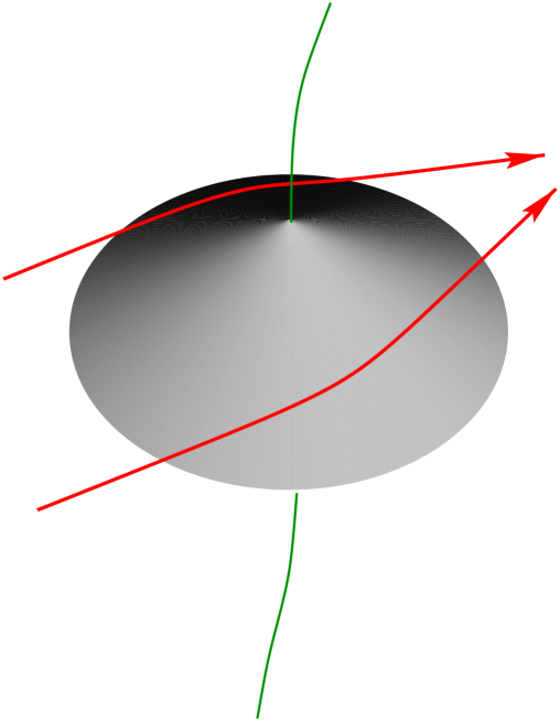
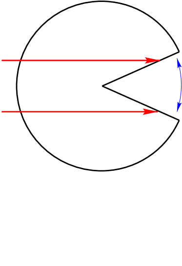
Figure 3.4: Surface à $t$ et $z$ constant de la métrique autour d’une corde cosmique sous critique ($\eta\ll M_{\mathrm{Pl}}$). L’angle manquant défléchit les rayons lumineux de $4\pi{\mathcal{G}}U$ indépendamment du paramètre d’impact.

Bien qu’il n’y ait pas d’effet statique, la géométrie de l’espace-temps autour d’une corde induit tout de même des effets gravitationnels potentiellement observables. Par exemple, les rayons lumineux issus d’une source lointaine peuvent être défléchis par la présence d’une corde entre la source et l’observateur [342, 162]. Dans le référentiel de la corde, et dans son plan perpendiculaire, l’angle de déflexion s’identifie clairement à l’angle manquant $\delta D\sim 8\pi{\mathcal{G}}U$ (cf. Fig. 3.4). Dans le cas général, avec $l$ et $d$ les distances de la corde à la source et à l’observateur respectivement, et $i$ l’angle d’inclinaison des rayons lumineux par rapport au plan perpendiculaire, il vient [341]

$$\delta D=\delta\theta\sin(i)\frac{l}{l+d}.$$ (3.66)

L’effet sur la matière est similaire. Deux particules de vitesse $v$ passant de part et d’autre de la corde vont acquérir une vitesse radiale l’une vers l’autre due à l’angle manquant de la métrique (cf. Fig. 3.4). Par projection sur la direction les reliant, il vient

$$\delta v\sim\gamma v\delta\theta$$ (3.67)

dans le référentiel d’une particule. Cet effet de sillage laissé par les cordes dans la matière environnante a été originellement considéré comme un autre mécanisme permettant de générer les perturbations gravitationnelles nécessaires à la formation des grandes structures (voir Chap. 1). Cependant, comme nous le verrons dans la partie II les contraintes cosmologiques actuelles semblent maintenant écarter ce scénario [11, 12, 27, 47, 98]. Les effets gravitationnels précédemment évoqués ne concernent cependant que les cordes rectilignes et sans structure interne. Or, nous verrons dans le chapitre 5 que leur évolution cosmologique tend naturellement à leur donner une allure fractale aux petites échelles de distance. L’existence de cette sous-structure peut alors exacerber la déflexion lumineuse induite par la corde du fait de l’apparition de caustiques [34, 332] (voir Fig. 3.5). Les modèles plus réalistes de cordes que nous présenterons dans le chapitre 6 invoquent de plus l’existence de courants de particules pouvant également générer des effets gravitationnels observables [147] (voir Fig. 3.6).

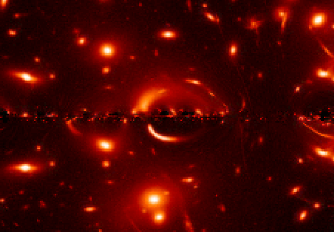
Figure 3.5: Effets simulés de lentille gravitationnelle induits par une corde cosmique possédant une allure de marche aléatoire aux petites échelles de distance. L’existence d’une telle micro-structrure est motivée par les simulations numériques d’évolution cosmologique de cordes (voir Chap. 5). L’image de fond est un amas de galaxies de redshift $z=1$ et la corde se trouve à $z=0.8$, pour une résolution angulaire inférieure à $0.1^{\prime\prime}$ [34].

Figure 3.6: Mouvement apparent des mirages gravitationnels générés par une corde cosmique suite au passage d’un pulse de courant de genre lumière. Dans la configuration d’observation (figure de gauche), le temps caractéristique de déplacement est $\ell{\mathcal{G}}U$ pour une source située à l’infini ($d\gg\ell$). Ainsi, pour une corde de grande unification (${\mathcal{G}}U\simeq 10^{-6}$) située à quelques mégaparsecs, le mouvement des images doubles de la source s’effectuerait pendant quelques années sur une ouverture angulaire maximale de $0.1^{\prime\prime}$ [147].

Les transitions de phase survenant dans l’univers primordial telles qu’elles sont prédites par le modèle standard de physique des particules peuvent donc générer des défauts topologiques comme les murs de domaine, les cordes cosmiques ou les monopôles. Comme nous le verrons dans les chapitres suivants, leur existence peut modifier significativement la dynamique de l’univers, et les contraintes cosmologiques s’imposant sur ces objets se trouvent finalement être des contraintes fortes sur les symétries qu’il a été possible de briser dans l’univers primordial. L’étude des défauts topologiques permet donc de sonder la physique des particules à des échelles d’énergie qu’il est impossible d’atteindre dans les accélérateurs.

3.4 Quelques contraintes

Les théories résumées dans ce chapitre permettent de résoudre certains problèmes des modèles standard, mais en posent de nouveaux, comme la formation des défauts topologiques. Il est de ce fait indispensable d’explorer ces conséquences afin de pouvoir mieux contraindre la nouvelle physique en jeu. Certains faits observationnels simples permettent déjà de situer les problèmes que pose l’existence de ces reliques de transition de phase.

La symétrie électrofaible comportant le groupe $U(1)$, dans une théorie de grande unification ce groupe doit faire partie de la chaîne de brisures de symétrie d’un groupe compact $G$. D’après (3.60), puisque $\pi_{1}\left[U(1)\right]\sim\mathbb{Z}$, il existe nécessairement un vide dans la chaîne tel que $\pi_{2}({\mathcal{V}})\nsim I$ menant à la formation de monopôles [289] (voir la section précédente). Le problème de ces objets est leur abondance: ils se comportent en effet comme de la matière ordinaire et l’évolution de leur densité rapportée à celle de l’entropie ne varie avec l’expansion que par leur annihilation avec des antimonopôles, également formés lors de la transition de phase. Or, ce taux d’annihilation est tel [371] qu’on peut montrer que, pour des monopôle de grande unification avec $\eta\sim 10^{15}\,{\mathrm{GeV}}$, leur densité actuelle dominerait la densité critique de plusieurs ordres de grandeur [289]. L’existence des monopôles n’est donc pas compatible avec le modèle standard cosmologique.

Si l’on s’intéresse aux murs de domaines, l’équation de Poisson du potentiel gravitationnel (3.62) se réduit à

$$\nabla^{2}V_{\mathrm{grav}}=-4\pi{\mathcal{G}}U,$$ (3.68)

avec $U$ la densité d’énergie surfacique du mur. La présence d’un tel défaut conduit donc à une force gravitationnelle répulsive, source d’effets détectables dans le CMBR à partir d’une échelle d’énergie de $\eta\sim 1\,{\mathrm{MeV}}$, c’est-à-dire largement en deça de la transition électrofaible [369, 211, 320]. Inversement, un mur de domaine formé lors de cette transition aurait une énergie $10^{8}$ fois supérieure à celle de toute la matière connue, et dominerait donc la dynamique de l’univers. La formation de ces défauts est donc également exclue par la cosmologie, et de ce fait la brisure d’une symétrie discrète par mécanisme de Higgs.

Une solution possible (et en fait privilégiée à l’heure actuelle) est celle de l’inflation. L’univers observable aujourd’hui provenant d’une région bien plus petite que l’horizon avant l’inflation, le facteur de dilution est considérable et la domination actuelle des reliques est évitée [166, 328]. Un autre mécanisme fait appel aux cordes cosmiques. Lors de transitions de phases ultérieures, des cordes peuvent être formées et se connecter aux autres défauts alors présents. Elles catalysent ensuite leur désintégration évitant ainsi la catastrophe cosmologique [222, 96, 184].

Les cordes de Kibble sont actuellement compatibles avec les contraintes observationnelles, et ce n’est que dans des effets plus fin que leur existence pourra être, ou non, infirmée. L’observation de la surface de dernière diffusion au travers du spectre de puissance du CMBR est actuellement un des moyens les plus prometteurs pour contraindre ces modèles. En effet, l’observation du rayonnement de fond diffus dans toutes les directions $\vec{u}$ du ciel permet d’en mesurer le contraste de température $\delta\Theta/\Theta$. La statistique de ces fluctuations est alors donnée par la connaissance de ses fonctions de corrélation. À l’ordre dominant, la fonction de corrélation à deux points est habituellement développée sur la base des polynômes de Legendre

$$\overline{\left(\left.\frac{\delta\Theta}{\Theta}\right|_{\vec{u}_{1}}\left.\frac{\delta\Theta}{\Theta}\right|_{\vec{u}_{2}}\right)}=\frac{1}{4\pi}\sum_{\ell=2}^{\infty}C_{\ell}P_{\ell}(\cos\theta),$$ (3.69)

où $\overline{()}$ désigne la valeur moyenne sur toutes les paires $(\vec{u}_{1},\vec{u}_{2})$ d’écart angulaire $\theta$. Il est commode de décomposer le contraste de température sur les harmoniques sphériques

$$\left.\frac{\delta\Theta}{\Theta}\right|_{\vec{u}}=\sum_{\ell=2}^{\infty}\sum_{m=-\ell}^{\ell}a_{\ell m}Y_{\ell}^{m}(\vec{u}),$$ (3.70)

où moments multipolaires $C_{\ell}$ se réduisent à

$$C_{\ell}=\frac{1}{2\ell+1}\sum_{m}\left|a_{\ell m}\right|^{2}.$$ (3.71)

Le spectre de puissance des fluctuations est finalement donnée par la dépendance en $\ell$ des moments $C_{\ell}$. Sur la figure 3.7 sont représentées les courbes de puissance prédites par différents modèles d’inflation, ainsi que celles produites par des défauts topologiques de type textures. La présence d’oscillations dans les prédictions des modèles inflationnaires, qui se retrouvent dans les observations (voir Fig. 3.8), semble être une confirmation supplémentaire du mécanisme d’inflation, initialement introduit pour résoudre le problème de l’horizon et de la platitude.

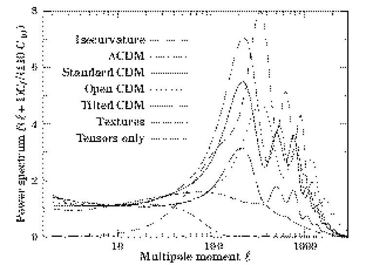
Figure 3.7: Le spectre de puissance des anisotropies de température dans le CMBR prédit par différentes théories d’inflation, et par des défauts topologiques de type textures [164]. La présence d’oscillations est observée dans les données actuelles (voir Fig. 3.8).

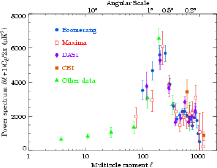
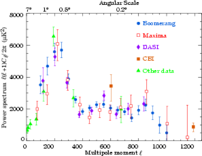
Figure 3.8: Le spectre de puissance des anisotropies de température dans le CMBR observé actuellement [164].

Les cordes cosmiques sont également des sources actives pouvant générer des fluctuations de température dans le CMBR. La métrique conique induisant des variations de vitesse relative des particules dans le sillage de la corde [cf. Eq. (3.67)], il est en de même pour les photons du CMBR [197, 162, 336, 47]. La présence de cordes cosmiques doit donc induire des fluctuations de température de l’ordre de

$$\overline{\left(\frac{\delta\Theta}{\Theta}\right)}_{2}\simeq\overline{\left(\delta v\right)}_{2}\simeq{\mathcal{G}}U,$$ (3.72)

où $\overline{\left(\right)}_{2}$ désigne la moyenne quadratique. Pour des cordes de grande unification ${\mathcal{G}}U\simeq 10^{-6}$ et l’ordre de grandeur de ces fluctuations est aussi celui qui est observé. Bien que le spectre de puissance généré par un réseau de cordes cosmiques locales dans FLRW ne soit pas encore bien connu, le mécanisme de génération des fluctuations est par nature incohérent [242, 347, 123, 124] et ne peut mener à la présence des pics tels qu’ils sont observés (voir Fig. 3.8). Sur la figure 3.7, l’évolution des moments multipolaires des textures s’effondre rapidement à grands $\ell$, et on peut s’attendre à un comportement similaire pour des cordes cosmiques. La présence d’un réseau de cordes cosmiques sans phase d’inflation est donc exclue par ces observations. Néanmoins, leur coexistence semble mieux s’accorder à tout point de vue. D’une part, le mécanisme d’inflation lui-même peut donner naissance à des cordes [287, 240], et le devenir de l’inflaton peut également conduire à des transitions de phase les générant. Sur la figure 3.9 est représentée le meilleur ajustement des données actuelles par un mélange des spectres de puissance issus des défauts topologiques et de l’inflation. Bien que la dégénérescence dans les paramètres soit importante, il est intéressant de noter que les données observationnelles sont mieux ajustées par un tel mélange que par un pur modèle d’inflation [48].

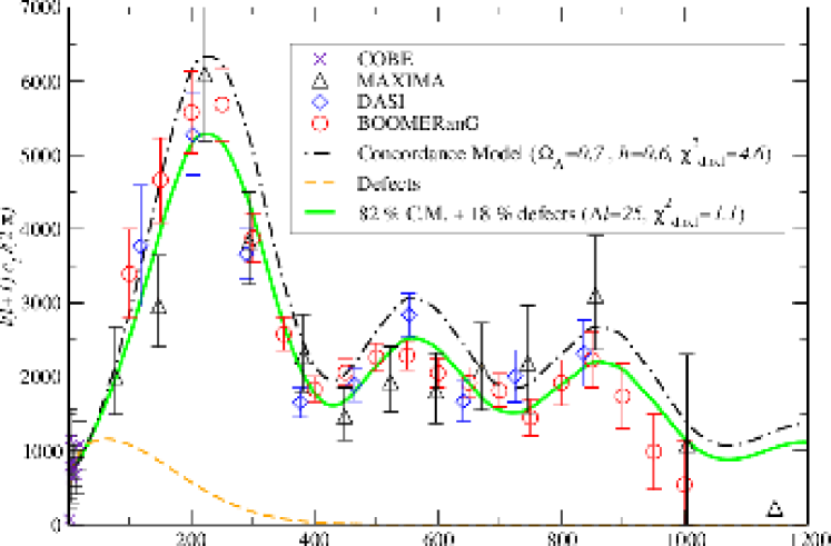
Figure 3.9: Spectre de puissance des fluctuations du CMBR prédit par la coexistence d’une phase d’inflation avec des défauts topologiques globaux. La proportion donnant le meilleur ajustement est également indiquée [48].

3.5 Conclusion

L’utilisation de la physique des hautes énergies en cosmologie permet de résoudre certains problèmes de taille du modèle standard de FLRW (problème de l’horizon, de la platitude …). Cependant, cette physique pose de nouveaux problèmes cosmologiques comme la formation de défauts topologiques dont font parties les cordes cosmiques. En plus de leur influence potentielle sur l’évolution de l’univers, le statut de leur existence est d’un intérêt direct pour la physique des particules du fait des contraintes qu’elle impose sur les symétries pouvant être brisées dans l’histoire de l’univers. Comme nous le verrons dans les parties II et III, il est possible d’étendre ces contraintes aux couplages que peut avoir le champ de Higgs formant la corde aux autres particules. De telles cordes s’habillent en effet de courants de charges modifiant leurs propriétés microscopiques et par voie de conséquence leur évolution cosmologique. La physique à l’œuvre dans ces cordes est plutôt complexe, et il est d’usage d’utiliser un formalisme macroscopique unifié pour les décrire. Dans la partie II, ce formalisme sera détaillé et appliqué pour des cordes de Kibble avec et sans courants bosoniques. Il rend possible la résolution des équation du mouvement et l’étude numérique de l’évolution des réseaux de cordes. De telles simulations seront présentées pour des cordes sans courant, et sont attendues pour statuer de manière rigoureuse sur la proportion de tels défauts présents dans les données du CMBR. L’étude cosmologique des cordes conductrices est pour sa part une tâche plus ardue par la complexité de la dynamique induite. Bien qu’encore applicable pour les courants de bosons, le formalisme macroscopique semble être moins adapté à la description des courants fermioniques (voir partie III). Néanmoins, nous verrons que la seule étude microscopique des cordes conductrices donne déjà des contraintes fortes sur la physique des hautes énergies en jeu dans l’univers primordial.

Deuxième partie Dynamique des cordes cosmiques

Chapitre 4 Formalismes macroscopiques

4.1 Introduction

Dans la partie I, la théorie microscopique minimale menant à la formation de cordes cosmiques par le mécanisme de Higgs introduisait deux champs bosoniques: le champ de Higgs $\Phi$ et le champ vectoriel $B_{\mu}$ associé à l’invariance de jauge $U(1)$. Les solutions de corde aux équations de champs sont généralement compliquées [voir Eqs. (3.42) et (3.43)] et il est souvent impossible de les déterminer autrement que par des méthodes numériques [282, 23, 303]. Il est par conséquent utile de se placer dans la limite de corde d’épaisseur nulle. Une telle approximation revient donc à ne plus se soucier de la structure interne de la corde, i.e. du profil transverse de ses champs (cf. Fig. 3.3), en la décrivant comme une $2$-surface de l’espace-temps. Lorsque le choix d’un référentiel est privilégié, ce qui est généralement le cas lorsque l’on s’intéresse au mouvement de la corde ou à ses couplages gravitationnels, il est commode de choisir un système de coordonnées internes $\xi^{a}$ en fonction duquel les grandeurs physiques peuvent être calculées: il s’agit du formalisme dit traditionnel qui sera détaillé dans la section 4.2. Néanmoins, certaines propriétés dues à la structure interne des cordes peuvent modifier complètement leur dynamique, comme par exemple l’existence de courants de particules s’y propageant. Il est possible de tenir compte de ces effets par le biais d’une équation d’état reliant la densité d’énergie $U$ à la tension de la corde $T$ dans un formalisme covariant [80, 71, 70, 63]. Ce dernier est en effet particulièrement adapté à la description des propriétés intrinsèques à chaque corde. Il permet en outre de discuter, d’un point de vue classique, sur la stabilité de ces objets en présence ou non de courants.

4.2 Cordes de Goto-Nambu

Le fait de négliger complètement la structure interne d’une corde impose une invariance de Lorentz longitudinale et celle-ci peut être représentée par une $2$-surface d’univers évoluant dans l’espace-temps dont le mouvement est décrit par la donnée des ses coordonnées

$$x^{\mu}=x^{\mu}\left(\xi^{a}\right).$$ (4.1)

Les paramètres $\xi^{a}$ sont les coordonnées internes à la corde, avec $a\in\{0,1\}$, dont la composante $a=0$ est choisie de genre temps et $a=1$ de genre espace. Ces coordonnées permettent de définir un lagrangien de surface caractérisant la dynamique propre de la corde [341]. Ce lagrangien $\overline{\mathcal{L}}_{\mathrm{gn}}$ doit être invariant sous les transformations de coordonnées de l’espace-temps $\delta x^{\mu}$ et de la $2$-surface $\delta\xi^{a}$. Il a de plus la dimension d’une masse au carré, et peut être identifié à la densité linéique d’énergie de la corde $U$. Sur la $2$-surface d’univers courbe, il vient l’action de Goto-Nambu [161, 261]

$$\overline{\mathcal{S}}_{\mathrm{gn}}=-U\int{{\mathrm{d}}^{2}\xi}\sqrt{-\gamma},$$ (4.2)

avec $\gamma$ le déterminant de la métrique induite sur la corde

$$\gamma_{ab}=g_{\mu\nu}\frac{\partial x^{\mu}}{\partial\xi^{a}}\frac{\partial x^{\nu}}{\partial\xi^{b}},$$ (4.3)

telle que

$${\mathrm{d}}s^{2}=g_{\mu\nu}\,{\mathrm{d}}x^{\mu}{\mathrm{d}}x^{\nu}=\gamma_{ab}\,{\mathrm{d}}\xi^{a}{\mathrm{d}}\xi^{b},$$ (4.4)

pour deux points sur la corde séparés par ${\mathrm{d}}x^{\mu}$ ou ${\mathrm{d}}\xi^{a}$. La normalisation du lagrangien de Goto-Nambu à $\overline{\mathcal{L}}_{\mathrm{gn}}=-U$ est en accord avec la définition du tenseur énergie impulsion obtenu par minimisation de l’action (4.2) par rapport à la métrique $g_{\mu\nu}$:

$$\sqrt{-g}\,T^{\mu\nu}=2\frac{\delta\overline{\mathcal{S}}_{\mathrm{gn}}}{\delta g_{\mu\nu}}=U\int{{\mathrm{d}}\xi^{2}}\sqrt{-\gamma}\,\gamma^{ab}\frac{\partial x^{\mu}}{\partial\xi^{a}}\frac{\partial x^{\nu}}{\partial\xi^{b}}\,\delta^{4}\left[{\mathbf{x}}-{\mathbf{x}}(\xi)\right],$$ (4.5)

où la fonction $\delta$ localise la corde dans l’espace-temps de référence. Pour une corde droite à symétrie cylindrique dans un espace-temps de Minkowski, en choisissant les coordonnées internes $\xi^{0}=x^{0}=t$ et $\xi^{1}=x^{3}=z$, il vient, par intégration sur les variables transverses,

$$\int{T^{tt}\,{\mathrm{d}}x_{\perp}^{2}}=U=-\int{T^{zz}\,{\mathrm{d}}x_{\perp}^{2}}=T.$$ (4.6)

Les cordes de Goto-Nambu suivent donc une équation d’état identique à celle obtenue dans le modèle de Higgs abélien, i.e. $U=T$. Les équations du mouvement donnant explicitement la trajectoire de la corde dans l’espace de référence, i.e. les fonctions $x^{\mu}$, sont obtenues à partir des équations d’Euler-Lagrange issues de l’action de Goto-Nambu. On trouve

$$\partial_{a}\left(\sqrt{-\gamma}\,\gamma^{ab}\,\partial_{b}x^{\mu}\right)+\Gamma^{\mu}_{\nu\rho}\sqrt{-\gamma}\,\gamma^{ab}\frac{\partial x^{\nu}}{\partial\xi^{a}}\frac{\partial x^{\rho}}{\partial\xi^{b}}=0,$$ (4.7)

les $\Gamma^{\mu}_{\nu\rho}$ étant les symboles de Christoffel de la métrique $g_{\mu\nu}$. En espace-temps plat, celles-ci se simplifient en

$$\partial_{a}\left(\sqrt{-\gamma}\,\gamma^{ab}\,\partial_{b}x^{\mu}\right)=0.$$ (4.8)

L’invariance sous les transformations de coordonnées internes requiert un choix de jauge supplémentaire. On choisit généralement les conditions de jauge conforme [341]:

$$\dot{{\mathbf{x}}}\cdot{\mathbf{x}}^{\prime}=0,\quad\dot{{\mathbf{x}}}^{{}^{2}}+{\mathbf{x}}^{\prime^{2}}=0,$$ (4.9)

où le point désigne la dérivée par rapport à $\xi^{0}$ et le prime par rapport à $\xi^{1}$. Les équations du mouvement (4.8) se réduisent alors à

$$\ddot{{\mathbf{x}}}+{\mathbf{x}}^{\prime\prime}=0.$$ (4.10)

Ce choix de jauge n’est pas encore suffisant, et le degré de liberté restant doit être fixé. Cela peut se faire, par example, en se plaçant dans la jauge transverse, définie par

$$\xi^{0}=x^{0}=t,\quad\xi^{1}=\xi.$$ (4.11)

Les conditions de jauge conforme (4.9) deviennent alors

$$\dot{\vec{x}}^{\,\raisebox{-1.0pt}[0.0pt][0.0pt]{\tiny}}\cdot\vec{x}^{\,{}^{\prime}\raisebox{2.2pt}[0.0pt][0.0pt]{\tiny}}=0,\quad\dot{\vec{x}}^{\,\raisebox{-1.0pt}[0.0pt][0.0pt]{\tiny 2}}+\vec{x}^{\,{}^{\prime}\raisebox{2.2pt}[0.0pt][0.0pt]{\tiny 2}}=1.$$ (4.12)

Le choix des coordonnées (4.9) permet donc, d’après (4.12), de s’affranchir de la composante de vitesse longitudinale qui est sans signification physique du fait de l’invariance de Lorentz dans cette direction. La dernière égalité dans l’équation (4.12) est juste un choix de normalisation fixant l’abscisse curviligne $\xi$. Dans ces conditions, les équations du mouvement (4.10) se simplifient encore en

$$\ddot{\vec{x}}^{\,\raisebox{-1.0pt}[0.0pt][0.0pt]{\tiny}}-\vec{x}^{\,{}^{\prime\prime}\raisebox{2.2pt}[0.0pt][0.0pt]{\tiny}}=0,$$ (4.13)

dont les solutions générales sont la propagation, à la vitesse de la lumière, des déformations de la corde

$$\vec{x}(t,\xi)=\frac{1}{2}\left[\vec{p}(\xi-t)+\vec{q}(\xi+t)\right],$$ (4.14)

avec

$$\vec{p}^{\,{}^{\prime}\raisebox{2.2pt}[0.0pt][0.0pt]{\tiny 2}}=\vec{q}^{\,{}^{\prime}\raisebox{2.2pt}[0.0pt][0.0pt]{\tiny 2}}=1.$$ (4.15)

Cette dernière équation résulte de la normalisation de $\xi$ choisie dans la jauge conforme. La masse de la corde est donnée, d’après (4.5), par

$$M=\int{{\mathrm{d}}\vec{x}^{{}^{3}}}T^{tt}=U\int{{\mathrm{d}}\xi},$$ (4.16)

assurant sa proportionnalité avec l’abscisse curviligne $\xi$. D’autre part, la courbure de la corde étant donnée par ${\mathrm{d}}^{2}\vec{x}/{\mathrm{d}}\xi^{2}$, elle est d’après (4.13), proportionnelle à l’accélération $\ddot{\vec{x}}^{\,\raisebox{-1.0pt}[0.0pt][0.0pt]{\tiny}}$ dans le référentiel de repos où la vitesse transverse $\dot{\vec{x}}^{\,\raisebox{-1.0pt}[0.0pt][0.0pt]{\tiny}}=0$. Ainsi, le mouvement de la corde tend à chaque instant à la rendre droite. La conservation de l’impulsion implique que la corde va finalement osciller en chacun de ses points autour de sa position d’équilibre rectiligne.

Jusqu’à présent, nous avons uniquement considéré des cordes infinies. Cependant, la description lagrangienne étant purement locale, les équations du mouvements obtenues s’appliquent tout aussi bien à des configurations de cordes fermées, ou boucles. Celles-ci représentent en fait la forme dominante sous laquelle les cordes évoluent après la transition de phase (cf. Chap. 5). La topologie fermée impose cependant des conditions périodiques à la propagation des perturbations, de la forme

$$\vec{x}(\xi+L)=\vec{x}(\xi),$$ (4.17)

où $L$ désigne la longueur propre totale de la boucle, i.e. $L=M/U$. Cette condition ne peut être vérifiée d’après (4.14) que si

$$\vec{p}(\xi+L)=\vec{p}(\xi),\quad\textrm{et}\quad\vec{q}(\xi+L)=\vec{q}(\xi),$$ (4.18)

autrement dit le mouvement de la boucle doit également être périodique dans le temps. Il est ainsi possible de développer les vecteurs $\vec{p}$ et $\vec{q}$ en série de Fourier dont les coefficients doivent vérifier la condition de normalisation (4.15) montrant que les vecteurs $\vec{p}^{\,{}^{\prime}\raisebox{2.2pt}[0.0pt][0.0pt]{\tiny}}$ et $\vec{q}^{\,{}^{\prime}\raisebox{2.2pt}[0.0pt][0.0pt]{\tiny}}$ évoluent sur une sphère de rayon unité. Si l’on s’intéresse à la vitesse des perturbations de courbure, en dérivant l’équation (4.14) il vient

$$\dot{\vec{x}}^{\,\raisebox{-1.0pt}[0.0pt][0.0pt]{\tiny 2}}=\frac{1}{4}\left[\vec{p}^{\,{}^{\prime}\raisebox{2.2pt}[0.0pt][0.0pt]{\tiny}}(\xi-t)-\vec{q}^{\,{}^{\prime}\raisebox{2.2pt}[0.0pt][0.0pt]{\tiny}}(\xi+t)\right]^{2},$$ (4.19)

et les points pour lesquels $\vec{p}^{\,{}^{\prime}\raisebox{2.2pt}[0.0pt][0.0pt]{\tiny}}(\xi-t)=-\vec{q}^{\,{}^{\prime}\raisebox{2.2pt}[0.0pt][0.0pt]{\tiny}}(\xi+t)$ vérifient $\dot{\vec{x}}^{\,\raisebox{-1.0pt}[0.0pt][0.0pt]{\tiny 2}}=1$. L’existence de tels points est générique du fait des conditions de périodicité (4.18) qui impliquent

$$\int_{0}^{L}\vec{p}^{\,{}^{\prime}\raisebox{2.2pt}[0.0pt][0.0pt]{\tiny}}\,{\mathrm{d}}\xi=\int_{0}^{L}\vec{q}^{\,{}^{\prime}\raisebox{2.2pt}[0.0pt][0.0pt]{\tiny}}\,{\mathrm{d}}\xi=0.$$ (4.20)

Autrement dit, les vecteurs $\vec{p}^{\,{}^{\prime}\raisebox{2.2pt}[0.0pt][0.0pt]{\tiny}}$ et $\vec{q}^{\,{}^{\prime}\raisebox{2.2pt}[0.0pt][0.0pt]{\tiny}}$ ne restent généralement pas dans un seul hémisphère de la sphère de rayon unité (4.15) assurant de ce fait leur intersection en certains points. La vitesse de ces points sur la corde est donc égale à celle de la lumière, et à partir du développement de Fourier des vecteurs $\vec{p}$ et $\vec{q}$ en leur voisinage, il est possible de montrer [208, 330] qu’ils correspondent à des points de rebroussement dans la forme de la corde. De telles discontinuités de courbure peuvent être à l’origine de l’émission de rayonnement, de particules si la corde est traversée de courant (cf. Chap. 6), et généralement d’ondes gravitationnelles potentiellement détectables [101]. Le mouvement d’oscillation, et la présence de points de rebroussement permettent aux boucles d’évacuer de l’énergie sous forme de rayonnement gravitationnel. En première approximation, en supposant l’énergie gravitationnelle ${\mathcal{E}}$ émise par le seul moment quadrupolaire $Q\simeq ML^{2}$, il vient [145]

$$\frac{{\mathrm{d}}{\mathcal{E}}}{{\mathrm{d}}t}\simeq{\mathcal{G}}\left(\frac{\delta^{3}Q}{\delta t^{3}}\right)^{2}\simeq{\mathcal{G}}Q^{2}\nu^{6},$$ (4.21)

où $\nu$ est la fréquence caractéristique des oscillations de la boucle, dont un ordre de grandeur est donné par $\nu\simeq 1/L$. De manière générale $\dot{{\mathcal{E}}}\simeq\gamma_{\mathrm{g}}{\mathcal{G}}U^{2}$ où $\gamma_{\mathrm{g}}$ est sans dimension et tient compte des écarts à l’équation (4.21). Le temps de vie d’une boucle est alors

$$\tau\simeq\frac{M}{\dot{{\mathcal{E}}}}\simeq\frac{1}{\gamma_{\mathrm{g}}}\frac{L}{{\mathcal{G}}U}.$$ (4.22)

Le coefficient de proportionnalité peut être estimé numériquement et est voisin de $\gamma_{\mathrm{g}}\simeq 65$ [14]. Comme nous le verrons dans le chapitre 5, la désintégration gravitationnelle des boucles est déterminante dans l’évolution et l’existence de réseaux de cordes cosmiques dans l’univers.

4.3 Formalisme covariant

La description précédente est particulièrement adaptée au cordes cosmiques sans structure interne, de Goto-Nambu. Cependant, comme nous le verrons dans les chapitres suivants, des courants peuvent prendre naissance sur les cordes. Un formalisme covariant, développé par B. Carter [80, 71, 70, 63], permet de tenir compte de ces nouveaux paramètres internes dans la dynamique de la corde uniquement au travers d’une équation d’état reliant la densité d’énergie $U$ à la tension $T$.

4.3.1 Géométrie des $2$-surfaces

L’évolution de la surface d’univers de la corde $x^{\mu}\left(\xi^{a}\right)$ nous a permis, dans la section précédente, de définir la métrique $\gamma_{ab}$ induite sur la corde [voir. Eq. (4.3)]. La corde peut, d’une façon générale, être considérée comme une variété de dimension $p=2$ immergée dans un espace de dimension supérieure $n=4$. En inversant la relation (4.3) il est possible de définir le premier tenseur fondamental de la corde

$${\P}^{\mu\nu}=\gamma^{ab}\partial_{a}x^{\mu}\partial_{b}x^{\nu}_{,}$$ (4.23)

où la dérivation partielle porte sur les coordonnées internes $\xi^{a}$. Par construction, ce tenseur vit sur la surface d’univers de la corde et en est donc un projecteur défini sur l’espace-temps de métrique $g_{\mu\nu}$. Le projecteur orthogonal s’obtient directement à partir de (4.23)

$$\perp^{\mu}_{\ \nu}=g^{\mu}_{\ \nu}-{\P}^{\mu}_{\ \nu},$$ (4.24)

et il vient

$${\P}^{\mu}_{\ \rho}{\P}^{\rho}_{\ \nu}={\P}^{\mu}_{\ \nu},\qquad\perp^{\mu}_{\ \rho}\perp^{\rho}_{\ \nu}=\perp^{\mu}_{\ \nu},\qquad{\P}^{\mu}_{\ \rho}\perp^{\rho}_{\ \nu}=0.$$ (4.25)

Le premier tenseur fondamental ${\P}^{\mu\nu}$ permet de se restreindre aux propriétés intrinsèques de la $2$-surface tout en conservant une approche covariante. Dans cet esprit, il est également commode d’introduire une dérivée covariante ${\overline{\nabla}}_{\mu}$ n’agissant que sur la surface d’univers décrite par la corde. Une manière naturelle de l’introduire est de la définir comme la composante tangentielle de la dérivée covariante usuelle sur la $2$-surface, i.e.

$${\overline{\nabla}}_{\mu}={\P}^{\nu}_{\ \mu}\nabla_{\nu}.$$ (4.26)

La structure géométrique de la corde peut alors être caractérisée par les variations de son premier tenseur fondamental avec les coordonnées internes. La formulation covariante associée met en jeu le deuxième tenseur fondamental

$${K_{\mu\nu}}^{\rho}={\P}^{\sigma}_{\ \nu}{\overline{\nabla}}_{\mu}{\P}^{\rho}_{\ \sigma}.$$ (4.27)

Plus précisément, s’il existe des quadrivecteurs $u^{\mu}$ et $v^{\mu}$ de genre temps et espace, respectivement, formant une base locale orthonormée de la $2$-surface

$$u^{\mu}u_{\mu}=-v^{\mu}v_{\mu}=1,\quad u^{\mu}v_{\mu}=0,$$ (4.28)

alors le premier tenseur fondamental devient, dans ce référentiel privilégié,

$${\P}^{\mu}_{\ \nu}=u^{\mu}u_{\nu}-v^{\mu}v_{\nu},$$ (4.29)

et selon l’équation (4.27) le deuxième tenseur fondamental se réduit à

$${K_{\mu\nu}}^{\rho}=\perp^{\rho}_{\ \sigma}\left(u_{\nu}{\overline{\nabla}}_{\mu}u^{\sigma}-v_{\nu}{\overline{\nabla}}_{\mu}v^{\sigma}\right).$$ (4.30)

La projection orthogonale à la corde de l’accélération du quadrivecteur unité $u^{\mu}$ s’obtient alors à partir de (4.30)

$$\perp^{\rho}_{\ \mu}\left(u^{\nu}{\overline{\nabla}}_{\nu}u^{\mu}\right)={K_{\mu\nu}}^{\rho}u^{\mu}u^{\nu}.$$ (4.31)

Le deuxième tenseur fondamental caractérise ainsi la forme géométrique de la corde dans les dimensions transverses. Il possède également des propriétés de symétrie nécessaire à la description de la corde comme une $2$-surface [66]

$${K_{[\mu\nu]}}^{\rho}=0.$$ (4.32)

Sa trace permet de plus de définir le vecteur de courbure extrinsèque

$$K^{\rho}={{K^{\mu}}_{\mu}}^{\rho}={\overline{\nabla}}_{\mu}{\P}^{\mu\rho},$$ (4.33)

qui s’exprime à partir de la métrique induite (4.3) et des connexions de l’espace-temps via

$$K^{\mu}=\frac{1}{\sqrt{-\gamma}}\partial_{a}\left(\sqrt{-\gamma}\gamma^{ab}\partial_{b}x^{\mu}\right)+\Gamma^{\mu}_{\nu\rho}\gamma^{ab}\partial_{a}x^{\nu}\partial_{b}x^{\rho}.$$ (4.34)

Par comparaison avec l’équation (4.7), on voit que les équations du mouvement extrinsèque de la corde se ramènent simplement à $K^{\mu}=0$ pour des cordes de Goto-Nambu. La détermination de celui-ci, dans le cas général, nécessite néanmoins la connaissance de la dynamique interne à la corde, ce qui peut se faire au moyen du lagrangien effectif de surface.

4.3.2 Lois de conservation

Comme dans le cas de Goto-Nambu, la métrique induite (4.3) permet de définir une action de surface décrivant les propriétés physiques intrinsèques à la corde. Le choix d’un lagrangien effectif $\overline{\mathcal{L}}$ est en général motivé par la théorie des champs sous-jacente et les divers couplages entre le champ de Higgs formant la corde et les champs externes. En plus des éventuelles symétries de jauge imposées par les divers couplages choisis, l’invariance de l’action vis-à-vis des transformations infinitésimales de la métrique permet de définir le tenseur énergie impulsion associé. L’équation (3.4) devient sur la $2$-surface

$${\overline{T}}^{\mu\nu}=2\frac{\delta\overline{\mathcal{L}}}{\delta g_{\mu\nu}}+\overline{\mathcal{L}}\,{\P}^{\mu\nu}.$$ (4.35)

La conservation du tenseur énergie impulsion sur la surface d’univers est assurée par le théorème de Noether et peut être mis sous sa forme surfacique covariante

$${\overline{\nabla}}_{\mu}{\overline{T}}^{\mu\nu}={\overline{f}}^{\nu},$$ (4.36)

avec la condition tangentielle ${\perp^{\mu}}_{\nu}{\overline{T}}^{\nu\rho}=0$. La densité totale de force ${\overline{f}}^{\mu}$ sur la $2$-surface tient compte de l’effet des champs extérieurs dans la théorie effective, et éventuellement de l’interaction de la corde avec d’autres $p$-surfaces. Dans le cas d’une corde de Goto-Nambu, ${\overline{f}}^{\mu}$ est identiquement nul, alors que l’existence d’un champ vectoriel extérieur $A^{\mu}$, associé à une invariance $U(1)$, conduirait à une force de type électromagnétique ${\overline{f}}^{\mu}=F^{\mu\nu}{\overline{j}}_{\nu}$, le courant surfacique étant naturellement défini par ${\overline{j}}_{\mu}=\delta\overline{\mathcal{L}}/\delta A^{\mu}$. Lorsque l’on s’intéresse au mouvement extrinsèque de la corde, seule la projection orthogonale de (4.36) est déterminante. À partir des équations (4.24) et (4.26), et de la définition du deuxième tenseur fondamental (4.27), il vient [73]

$${\overline{\nabla}}_{\mu}\perp^{\nu}_{\ \rho}=-{K_{\mu\nu}}^{\rho}-K_{\mu\,\,\nu}^{\,\rho},$$ (4.37)

et la projection orthogonale de (4.36) est alors

$${\overline{T}}^{\mu\nu}{K_{\mu\nu}}^{\rho}=\perp^{\rho}_{\ \sigma}{\overline{f}}^{\sigma}.$$ (4.38)

La connaissance du tenseur énergie impulsion ${\overline{T}}^{\mu\nu}$ et des densités de force ${\overline{f}}^{\mu}$ permet ainsi de déterminer à l’aide des Eqs. (4.33) et (4.38), le vecteur de courbure extrinsèque, et par la relation (4.34) les équations du mouvement de la corde.

La forme générique du tenseur énergie impulsion d’une $2$-surface s’obtient en supposant que son énergie est bien définie, i.e. positive ou nulle, et que la causalité n’est pas violée, i.e. qu’il possède un vecteur propre tangentiel de genre temps $u^{\mu}$ vérifiant $u^{\mu}u_{\mu}>0$. La densité d’énergie est alors la valeur propre du tenseur énergie impulsion associée à $u^{\mu}$. En le normalisant à l’unité $u^{\mu}u_{\mu}=1$, il vient

$${\overline{T}}^{\mu}_{\ \nu}u^{\nu}=Uu^{\mu},$$ (4.39)

avec $U\geq 0$. Il est alors possible d’introduire un autre vecteur tangentiel $v^{\mu}$ de genre espace vérifiant (4.28) pour construire la base orthornormé introduite dans la section précédente. En supposant, dans cette base, le tenseur énergie impulsion diagonal, la tension $T$ de la corde est définie par

$${\overline{T}}^{\mu\nu}=Uu^{\mu}u^{\nu}-Tv^{\mu}v^{\nu},$$ (4.40)

soit, en fonction du premier tenseur fondamental (4.23)

$${\overline{T}}^{\mu\nu}=(U-T)u^{\mu}u^{\nu}+T\,{\P}^{\mu\nu}.$$ (4.41)

La dénomination de tension se justifie donc par analogie avec la forme hydrodynamique (1.10) où $T$ s’identifirait à $-P$, comme intuitivement attendu sur un banal fil en mécanique classique. En reportant l’expression (4.41) dans les équations du mouvement extrinsèque (4.38), il vient

$${\overline{T}}^{\mu\nu}{K_{\mu\nu}}^{\rho}=\perp^{\rho}_{\ \sigma}\left(U\dot{u}^{\sigma}-Tv^{\prime\sigma}\right)=\perp^{\rho}_{\ \sigma}{\overline{f}}^{\sigma},$$ (4.42)

avec l’accélération $\dot{u}^{\sigma}=u^{\mu}{\overline{\nabla}}_{\mu}u^{\sigma}$ et $v^{\prime\sigma}=v^{\mu}{\overline{\nabla}}_{\mu}v^{\sigma}$. Dans le cas où il n’y a pas de champ de force extérieur, ${\overline{f}}^{\mu}=0$ et le vecteur de courbure extrinsèque est alors donné par l’équation (4.33), qui à l’aide de (4.42), se simplifie en

$$K^{\rho}=\perp^{\rho}_{\ \sigma}\left(1-\frac{U}{T}\right)\dot{u}^{\sigma}.$$ (4.43)

Les corde de Goto-Nambu vérifiant $U=T$ possèdent donc un vecteur de courbure extrinsèque nul $K^{\rho}=0$ redonnant à partir de (4.34) les équations du mouvements (4.7). En fait, l’expression (4.41) du tenseur énergie impulsion ne peut être invariante sous les transformation de Lorentz longitudinales que si le terme en $u^{\mu}u^{\nu}$ s’annule, soit pour $U=T$. L’égalité entre la densité d’énergie et la tension est donc une conséquence directe de l’absence de structure interne le long de la corde. Réciproquement, en modifiant cette relation, il est possible de construire des modèles effectifs tenant compte des propriétés microscopiques rendant la structure interne non triviale. L’équation reliant $U$ à $T$ est alors une équation d’état pour la dynamique de la corde.

4.3.3 Équation d’état

La plus simple des équations d’état autre que celle de Goto-Nambu $U=T$ est celle régissant la dynamique d’une corde parfaitement élastique, ou barotropique, dont la densité d’énergie ne dépend que de la tension $U=U(T)$. Puisqu’une telle corde n’est plus invariante de Lorentz selon sa direction longitudinale, elle possède une structure interne qui doit être décrite par des paramètres physiques. À partir de l’équation d’état $U=U(T)$, il est en effet possible de définir le potentiel chimique ${\overline{\mu}}$ et un nombre de densité ${\overline{\nu}}$ tels que

$$\ln{{\overline{\nu}}}=\int{\frac{{\mathrm{d}}U}{U-T}},\qquad\ln{{\overline{\mu}}}=-\int{\frac{{\mathrm{d}}T}{U-T}}.$$ (4.44)

Par intégration de l’équation (4.44), le potentiel chimique et le nombre de densité apparaissent transformés de Legendre l’un de l’autre

$$U-T={\overline{\mu}}\,{\overline{\nu}}.$$ (4.45)

À partir des équations (4.41) et (4.45), le tenseur énergie impulsion de la corde barotropique devient

$${\overline{T}}^{\rho\sigma}={\overline{\nu}}^{\rho}{\overline{\mu}}^{\sigma}+T{\P}^{\rho\sigma},$$ (4.46)

où le vecteur densité de courant ${\overline{\nu}}^{\rho}$ et le flux d’énergie ${\overline{\mu}}^{\rho}$ sont définis par

$${\overline{\nu}}^{\rho}={\overline{\nu}}u^{\rho},\qquad{\overline{\mu}}^{\rho}={\overline{\mu}}u^{\rho}.$$ (4.47)

La dynamique de la corde est alors obtenue à l’aide de l’équation de conservation (4.36) avec, selon (4.46)

$${\overline{\nabla}}_{\rho}{\overline{T}}^{\rho}_{\ \sigma}={\overline{\mu}}_{\sigma}{\overline{\nabla}}_{\rho}{\overline{\nu}}^{\rho}+{\overline{\nu}}^{\rho}{\overline{\nabla}}_{\rho}{\overline{\mu}}_{\sigma}-{\overline{\nu}}^{\rho}{\overline{\nabla}}_{\sigma}{\overline{\mu}}_{\rho}+TK_{\sigma}.$$ (4.48)

Comme dans le cas de Goto-Nambu, les équations du mouvement extrinsèques sont obtenues en projetant (4.36) sur les dimensions transverses à l’aide de $\perp^{\rho}_{\ \sigma}$, alors que la dynamique interne est donnée par la composante longitudinale. En supposant la corde barotrope isolée, i.e. ${\overline{f}}^{\rho}=0$ dans l’équation (4.36), la divergence de ${\overline{T}}^{\rho}_{\ \sigma}$ est nulle, et par contraction de (4.48) avec la densité de courant ${\overline{\nu}}^{\sigma}$, il vient

$${\overline{\nu}}^{\sigma}{\overline{\nabla}}_{\rho}{\overline{T}}^{\rho}_{\ \sigma}=0\quad\Rightarrow\quad{\overline{\nabla}}_{\rho}{\overline{\nu}}^{\rho}=0.$$ (4.49)

Le quadrivecteur densité de courant est donc conservé. La relation (4.45) est caractéristique d’une corde cosmique parcourue par un courant conservé brisant l’invariance de Lorentz longitudinale. La conservation du flux d”énergie est également assurée par la projection longitudinale des équations de conservation (4.36), toujours pour le tenseur (4.46),

$${\P}^{\sigma}_{\ \alpha}{\overline{\nabla}}_{\rho}{\overline{T}}^{\rho}_{\ \sigma}=0\quad\Rightarrow\quad{\P}^{\sigma}_{\ \alpha}u^{\rho}{\overline{\nabla}}_{\left[\rho\right.}{\overline{\mu}}_{\left.\sigma\right]}=0.$$ (4.50)

Le potentiel chimique ${\overline{\mu}}$ peut alors être interprété comme la masse effective par particule à l’origine du courant conservé ${\overline{\nu}}^{\rho}$ le long de la corde [66, 73]. Comme nous le verrons dans le chapitre 6, ce modèle est particulièrement bien adapté à la description de cordes cosmiques possédant un condensât de Bose à l’origine d’un courant de particules scalaires [282, 281].

L’équation d’état permettant de connaître complètement la dynamique de la corde, il doit être également possible d’en dériver le lagrangien de surface en fonction des paramètres internes. Dans le cas barotrope, ${\overline{\mu}}$ et ${\overline{\nu}}$ étant reliés par l’équation d’état, il n’y a qu’un seul paramètre indépendant et ce lagrangien ne peut être fonction que d’une seule variable $\varpi$,

$$\overline{\mathcal{L}}={\overline{\Lambda}}(\varpi),$$ (4.51)

où ${\overline{\Lambda}}$ est génériquement non linéaire. D’après l’équation (4.50), le rotationnel du flux ${\overline{\mu}}^{\rho}$ s’annulant, celui-ci dérive d’un potentiel surfacique $\varphi$ tel que ${\overline{\mu}}_{\rho}={\overline{\nabla}}_{\rho}\varphi$. Ceci suggère, dans la représentation lagrangienne, de choisir un tel potentiel scalaire $\varphi$ comme paramètre interne indépendant, et d’imposer l’existence d’un courant conservé ${\overline{p}}^{\rho}$ tel que

$${\overline{p}}_{\rho}={\overline{\nabla}}_{\rho}\varphi.$$ (4.52)

Il existe alors un autre courant trivialement conservé ${\overline{c}}^{\sigma}=\varepsilon^{\sigma\rho}{\overline{p}}_{\rho}$ permettant de définir la variable $\varpi$

$$\varpi={\overline{c}}_{\rho}{\overline{c}}^{\rho}=-{\overline{p}}_{\rho}{\overline{p}}^{\rho}=-\gamma^{ab}\partial_{a}\varphi\partial_{b}\varphi.$$ (4.53)

L’identification de ces paramètres avec les variables physiques de la corde s’effectue naturellement à l’aide du tenseur énergie impulsion en comparant les équations (4.36) et (4.46). Pour cela, il est commode d’introduire les quantités duales

$${\widetilde{c}}^{\rho}=2\frac{{\mathrm{d}}{\overline{\Lambda}}}{{\mathrm{d}}\varpi}\,{\overline{p}}^{\rho},\quad{\widetilde{p}}_{\rho}=2\frac{{\mathrm{d}}{\overline{\Lambda}}}{{\mathrm{d}}\varpi}\,{\overline{c}}_{\rho},\quad\widetilde{\varpi}={\widetilde{c}}^{\rho}{\widetilde{c}}_{\rho}=-{\widetilde{p}}^{\rho}{\widetilde{p}}_{\rho},$$ (4.54)

ainsi que la fonction maîtresse duale

$${\widetilde{\Lambda}}={\overline{\Lambda}}-2\varpi\frac{{\mathrm{d}}{\overline{\Lambda}}}{{\mathrm{d}}\varpi}.$$ (4.55)

Le tenseur énergie impulsion (4.36) prend alors une forme symétrique

$${\overline{T}}^{\rho\sigma}=\frac{{\overline{\Lambda}}}{\varpi}\,{\overline{c}}^{\rho}{\overline{c}}^{\sigma}+\frac{{\widetilde{\Lambda}}}{\widetilde{\varpi}}\,{\widetilde{c}}^{\rho}{\widetilde{c}}^{\sigma},$$ (4.56)

et d’après l’équation (4.46), selon que le courant conservé ${\overline{c}}^{\rho}$ est de genre temps ou espace, les fonctions maîtresse ${\overline{\Lambda}}$ et ${\widetilde{\Lambda}}$ s’identifient à $-U$ et $-T$, ou $-T$ et $-U$ respectivement, alors que le paramètre d’état $\varpi$ est égal à $-{\overline{\nu}}^{2}$ ou ${\overline{\mu}}^{2}$ respectivement. La différenciation de ces deux régimes, respectivement désignés électrique et magnétique, résulte uniquement de la compatibilité du choix des quadrivecteurs de base $u^{\rho}$ et $v^{\rho}$ avec la définition du quadrivecteur courant ${\overline{c}}^{\rho}$. L’action de Goto-Nambu (4.2) est trivialement retrouvée dans la limite de courant nul $\varpi\rightarrow 0$ où $\overline{\mathcal{L}}=-U=-T$ indépendamment du régime.

4.3.4 Stabilité

En plus de décrire de manière unifiée les différentes propriétés microscopiques des cordes au travers d’une équation d’état, le formalisme covariant permet également de statuer sur la stabilité de celles-ci vis-à-vis de la propagation de perturbations transverses et longitudinales de leur géométrie. La propagation de perturbations transverses concerne évidemment la partie extrinsèque des équations du mouvement. La première équation est donnée par la condition d’intégrabilité (4.32) du tenseur de courbure extrinsèque. En la projetant orthogonalement à la surface d’univers, il vient à l’aide de l’équation (4.30),

$$\perp^{\beta}_{\ \rho}{K_{[\mu\nu]}}^{\rho}=0\quad\Leftrightarrow\quad\perp^{\beta}_{\ \rho}u^{\alpha}{\overline{\nabla}}_{\alpha}v^{\rho}=\perp^{\beta}_{\ \rho}v^{\alpha}{\overline{\nabla}}_{\alpha}u^{\rho}.$$ (4.57)

La deuxième équation est directement donnée par les équations du mouvement extrinsèques (4.42). Si maintenant on s’intéresse à la propagation de perturbations transverses de la géométrie de la forme

$$\delta u^{\rho}=\varepsilon(u^{\rho})\,{\mathrm{e}}^{i\chi},\qquad\delta v^{\rho}=\varepsilon(v^{\rho})\,{\mathrm{e}}^{i\chi},$$ (4.58)

de vecteur d’onde $k^{\sigma}$ défini par

$${\overline{\nabla}}_{\sigma}\chi=k_{\sigma},$$ (4.59)

les équations (4.42) et (4.57), pour les infiniments petits du premier ordre $\varepsilon$, deviennent

$$\begin{array}[]{lcl}\omega\perp^{\beta}_{\ \rho}\varepsilon(v^{\rho})+k\perp^{\beta}_{\ \rho}\varepsilon(u^{\rho})&=&0,\\ \\ \omega\,U\perp^{\beta}_{\ \rho}\varepsilon(u^{\rho})+k\,T\perp^{\beta}_{\ \rho}\varepsilon(v^{\rho})&=&0,\end{array}$$ (4.60)

où l’énergie et l’impulsion longitudinale des perturbations sont respectivement définies par

$$\omega=k_{\sigma}u^{\sigma},\qquad k=-k_{\sigma}v^{\sigma}.$$ (4.61)

La condition d’existence de solutions aux équations (4.60) donne alors la valeur de la vitesse des perturbations transverses

$$c_{{}_{\mathrm{T}}}^{2}=\frac{\omega^{2}}{k^{2}}=\frac{T}{U}.$$ (4.62)

Encore une fois, pour des cordes de Goto-Nambu, $c_{{}_{\mathrm{T}}}^{2}=1$ comme attendu par la résolution explicite des équations du mouvement donnée en (4.14). Dans le cas général, la tension $T$ doit être toujours positive pour que la corde soit transversalement stable. Si ce n’était pas le cas, il pourrait exister des régions où $c_{{}_{\mathrm{T}}}^{2}<0$, et les perturbations transverses (4.58) seraient exponentiellement amplifiées.

De la même manière l’existence d’une structure interne autorise la propagation de perturbations longitudinales le long de la corde. Ces ondes de type acoustique vont sur leur passage modifier les variables internes, i.e. ${\overline{\mu}}$ et ${\overline{\nu}}$ dans le cas barotrope. En plus des perturbations (4.58), il convient donc d’introduire

$$\delta{\overline{\nu}}=\varepsilon({\overline{\nu}})\,{\mathrm{e}}^{i\chi},\qquad\delta{\overline{\mu}}=\varepsilon({\overline{\mu}})\,{\mathrm{e}}^{i\chi},$$ (4.63)

avec, comme précédemment, $\varepsilon$ un infiniment petit du premier ordre. La projection longitudinale de la conservation du courant (4.49) donne la première équation

$${\P}^{\alpha}_{\ \rho}k_{\alpha}\left[{\overline{\nu}}\,\varepsilon(u^{\rho})+u^{\rho}\,\varepsilon({\overline{\nu}})\right]=0,$$ (4.64)

alors que la deuxième résulte de l’équation de conservation de l’énergie (4.50),

$$u^{\beta}k_{\beta}\,{\overline{\mu}}\,v^{\rho}\,\varepsilon(u_{\rho})-v^{\beta}k_{\beta}\,\varepsilon({\overline{\mu}})=0.$$ (4.65)

La vitesse de propagation des perturbations longitudinales se réduit donc, d’après (4.64) et (4.65), à

$$c_{{}_{\mathrm{L}}}^{2}=\frac{\omega^{2}}{k^{2}}=\frac{{\overline{\nu}}\,\varepsilon({\overline{\mu}})}{{\overline{\mu}}\,\varepsilon({\overline{\nu}})}.$$ (4.66)

Les paramètres internes ${\overline{\mu}}$ et ${\overline{\nu}}$ étant reliés par les relations de définition (4.44) et l’équation d’état (4.45), il vient finalement

$$c_{{}_{\mathrm{L}}}^{2}=-\frac{{\mathrm{d}}T}{{\mathrm{d}}U},$$ (4.67)

et la stabilité de la corde vis-à-vis des perturbations longitudinales requiert ${\mathrm{d}}T/{\mathrm{d}}U<0$.

Le formalisme macroscopique permet donc, à partir de l’équation d’état, de connaître la stabilité locale des cordes par rapport aux perturbations de leur mouvement, et de statuer sur leur existence potentielle. Il a été ainsi possible d’éliminer toute une classe de cordes caractérisées par une tension négative [278]. Ces critères de stabilité basés sur l’existence de vitesses de propagation physiques des perturbations ne sont cependant que nécessaires dans le cas des boucles de corde. La structure périodique induisant l’apparition d’une infinité de résonances, la stabilité de la boucle vis-à-vis des perturbations ne sera assurée que si la superposition de tous ces modes d’oscillations reste finie. Ce problème est d’autant plus important que la brisure de l’invariance de Lorentz longitudinale par l’existence d’une structure interne peut conduire à l’apparition d’anneaux stables de corde cosmique, appelés vortons [105, 54]. Comme pour des boucles de Goto-Nambu, la perte d’énergie par rayonnement gravitationnel se traduit par une diminution de la longueur propre des anneaux sous l’effet de leur tension. Cependant, l’existence d’un moment cinétique impose dans le même temps l’augmentation de leur vitesse angulaire jusqu’au moment où l’équilibre entre la tension et la force centrifuge est atteint (voir Fig. 4.1).

Figure 4.1: La brisure de l’invariance de Lorentz longitudinale par l’existence d’une structure interne permet l’existence de boucles stables de corde cosmique, les vortons. La tension est alors équilibrée par la force centrifuge lorsque la vitesse de rotation égale celle de propagation des perturbations extrinsèques $v^{2}=T/U$ [80, 71].

Si l’espace temps de référence est plat, dans le cas le plus simple d’un anneau circulaire de rayon $R$ et de vitesse angulaire $\dot{\theta}$, les quadrivecteurs de base $u^{\rho}$ et $v^{\rho}$ [cf. Eq. (4.28)] peuvent se mettre, en coordonnées cylindriques, sous la forme [79]

$$u^{\rho}=\left(\gamma_{\ell}\,v,0,\gamma_{\ell},0\right),\qquad v^{\rho}=\left(\gamma_{\ell},0,\gamma_{\ell}\,v,0\right),$$ (4.68)

avec le facteur de Lorentz $\gamma_{\ell}=1/\sqrt{1-v^{2}}$, et la vitesse de rotation $v=R\dot{\theta}$. En reportant (4.68) dans les équations du mouvement extrinsèque (4.42) en l’absence de force externe ${\overline{f}}^{\rho}=0$, il vient

$$v^{2}=c_{{}_{\mathrm{T}}}^{2}=\frac{T}{U},$$ (4.69)

comme intuitivement attendu par des considérations classiques (cf. Fig. 4.1). Il est alors possible de montrer que le critère de stabilité classique de tels anneaux vis-à-vis des divers modes de propagation des perturbations est encore donné par les valeurs des vitesses $c_{{}_{\mathrm{T}}}^{2}$ et $c_{{}_{\mathrm{L}}}^{2}$ [248, 247, 81]. Sur la figure 4.2 sont représentés en noir les domaines du plan $\left(c_{{}_{\mathrm{L}}}^{2},c_{{}_{\mathrm{T}}}^{2}\right)$ menant à des anneaux de corde instables [246]. Ainsi, les cordes cosmiques ayant une équation d’état de type subsonique, i.e. $c_{{}_{\mathrm{T}}}^{2}<c_{{}_{\mathrm{L}}}^{2}$, prédisent l’existence de vortons stables, alors que les modèles supersoniques où $c_{{}_{\mathrm{T}}}^{2}>c_{{}_{\mathrm{L}}}^{2}$ mènent à des vortons génériquement instables.

Figure 4.2: Domaines d’instabilité classiques (en noir) des anneaux de corde cosmique en fonction du carré des vitesses de propagation des perturbations transverses et longitudinales. Les boucles associées aux modèles de corde supersoniques $c_{{}_{\mathrm{T}}}^{2}>c_{{}_{\mathrm{L}}}^{2}$ sont donc génériquement instables [246].

4.4 Conclusion

La limite d’épaisseur nulle des cordes cosmiques permet donc, par le biais des formalismes macroscopiques, d’en déduire les caractéristiques essentielles de leur dynamique, ainsi que leur stabilité vis-à-vis des perturbations de leur forme. L’énergie par unité de longueur et la tension apparaissent comme les quantités physiques déterminantes dans la description de telles $2$-surfaces: l’équation d’état $U=U(T)$ fixe la dynamique propre de la corde alors que les valeurs des vitesses de propagation des perturbations $c_{{}_{\mathrm{T}}}^{2}=T/U$ et $c_{{}_{\mathrm{L}}}^{2}=-{\mathrm{d}}T/{\mathrm{d}}U$ en sont les critères de stabilité.

Cependant, les formalismes macroscopiques ne peuvent rendre compte des propriétés dues à la structure transverses du vortex, et les résultats précédents ne peuvent s’appliquer que si cette structure n’est pas déterminante dans les processus physiques à l’étude. Dans les cas contraires, il est alors nécessaire de recourir à des modèles microscopiques invoquant les champs formant la corde, et nécessitant le plus souvent l’emploi de méthodes numériques.

Comme nous le verrons dans les chapitres suivants les deux approches sont complémentaires et autorisent l’étude des cordes cosmiques du point de vue cosmologique tout en mettant en jeu les paramètres des théories de physique des particules responsables de leur formation.

Chapitre 5 Évolution cosmologique

5.1 Introduction

La microphysique des brisures de symétrie par le mécanisme de Higgs (voir chapitre 3) et les formalismes macroscopiques (voir chapitre 4) décrivent les propriétés physiques des cordes cosmiques prises individuellement. Cependant, dans l’univers primordial, les transitions de phase menant à leur formation, créent un réseau de cordes dans un univers de FLRW en expansion. Afin d’en étudier l’évolution cosmologique, il faut tout d’abord déterminer ses caractéristiques physiques initiales, puis les faire évoluer à partir de la connaissance de la dynamique et des interactions de chacune de ses cordes. Bien qu’il existe des modèles effectifs décrivant de tels réseaux [211, 210, 346], leur modélisation réaliste passe par l’emploi de simulations numériques [9, 33, 13, 308]. Initialement, ces simulations ont été développées dans les années 1980 pour calculer l’évolution de la densité d’énergie associée aux réseaux de cordes de Goto-Nambu, afin d’en déterminer leur impact sur la formation des grandes structures. D’une part, elles ont montré que ces réseaux étaient compatibles avec les contraintes cosmologiques à condition qu’une certaine partie de leur énergie soit évacuée sous forme de rayonnement, ce qui est effectivement réalisé par le biais de la désintégration gravitationnelle des boucles (voir Sect. 4.2). D’autres parts, il est apparu que les réseaux de cordes n’étaient pas l’effet dominant dans la formation des grandes structures. Aujourd’hui, ces codes d’évolution sont à nouveau à l’étude dans le but d’obtenir les signatures observationnelles que pourrait avoir l’existence d’un réseau [365], essentiellement dans les données actuelles et à venir concernant le CMBR [263, 35, 226, 323]. Dans cette optique, le plus précis des codes de l’époque, développé par F. Bouchet [33, 47], a été repris et modernisé à l’aide des avancées technologiques de la dernière décennie, en particulier par l’utilisation de méthode de parallélisation (voir annexe 11). Comme nous verrons dans la section 5.3.3, il est maintenant possible d’extraire le spectre de puissance du CMBR d’un univers possédant un réseau de cordes cosmiques.

5.2 Intercommutation

En plus du mouvement propre de chaque corde, la dynamique d’un réseau fait que les cordes vont nécessairement se croiser. Du point de vue de la topologie du vide, il est impossible de statuer sur l’issue d’une telle interaction: soit les cordes se traversent simplement, soit elles échangent leur branches. C’est la dynamique des champs formant le vortex qui va alors déterminer ce qui se passe effectivement. Les simulations numériques effectuées pour résoudre les équations de champs du type (3.42) et (3.43) pour deux vortex en interaction, obtiennent toutes que l’échange de partenaires est privilégié, que ce soit dans les intersections de cordes globales [314] ou locales [252, 257] (voir Fig. 5.1). Au vue de ces résultats, on estime que la probabilité d’intercommutation, i.e. d’échange des segments, est suffisamment proche de l’unité pour que l’on puisse considérer que cette reconnexion se produit systématiquement.

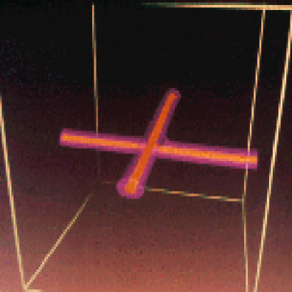
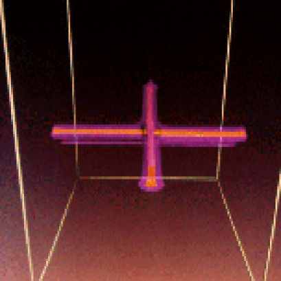
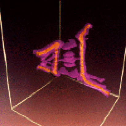
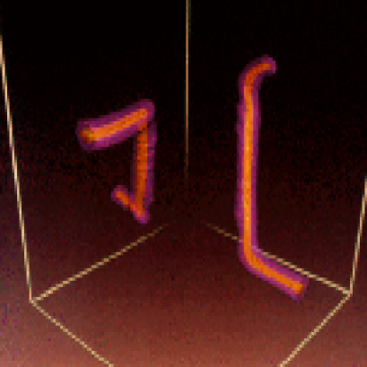
Figure 5.1: Intercommutation de deux cordes cosmiques dans le modèle de Higgs abélien [252]. Les cordes sont représentées par le profil transverse des champ de Higgs (en orange) et de jauge (en mauve), et après une phase intermédiaire d’excitation des divers champs, elles échangent leurs segments respectifs. La probabilité d’échange estimée par les diverses simulations numériques est $P_{\mathrm{e}}\simeq 1$.

Une conséquence majeure de ce mécanisme d’intercommutation est la formation incessante de boucles de cordes cosmiques. En effet, par ses oscillations (voir Sect. 4.2), une corde peut s’intercommuter avec elle même et échanger ses propres segments, menant ainsi à une nouvelle corde infinie accompagnée d’une boucle (voir Fig. 5.2). De même, une collision entre deux cordes différentes en deux points distincts conduit également à la formation d’un anneau constitué des segments de chaque corde (voir Fig. 5.2).

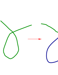
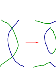
Figure 5.2: Formation de boucles de corde cosmique par intercommutation d’une seule corde, ou intersection de deux cordes différentes.

Dans la section 4.2, nous avons vu que les mouvements d’oscillation propres des boucles conduisent généralement à l’apparition de discontinuités dans la forme de la corde qui se propagent à la vitesse de la lumière. Un autre type de discontinuité apparaît également lors de l’intercommutation des cordes, comme on peut le voir sur la figure 5.1. La conservation de l’impulsion lors de l’intercommutation impose aux points de la nouvelle corde issus des deux cordes initiales (ou des deux zones différentes de la même corde), d’avoir des vitesses voisines de celles qu’ils avaient avant l’interaction. Autour du point d’échange, la nouvelle corde présente donc des variations de vitesse et de forme très rapides en fonction de l’abscisse curviligne $\xi$, qui, dans la limite d’épaisseur nulle, apparaissent comme des discontinuités dans les dérivées $\dot{\vec{x}}^{\,\raisebox{-1.0pt}[0.0pt][0.0pt]{\tiny}}(\xi,t)$ et $\vec{x}^{\,{}^{\prime}\raisebox{2.2pt}[0.0pt][0.0pt]{\tiny}}(\xi,t)$. Pour des cordes de Goto-Nambu, d’après l’équation (4.14), ces discontinuités, appelées kinks, correspondent également à des discontinuités des vecteurs $\vec{p}(\xi-t)$ et $\vec{q}(\xi+t)$, à $\xi-t$ et $\xi+t$ constants, respectivement. Autrement dit, ces kinks se propagent à la vitesse de la lumière dans chacune des directions de la corde à partir du point d’intercommutation. La propagation de ces ondes de discontinuité donne alors une forme plus ou moins “cisaillée” aux cordes ayant subi de multiples interactions. Comme les points de rebroussement, les kinks sont des sources d’ondes gravitationnelle intenses pouvant permettre leur éventuelle détection [101].

L’intercommutation est un mécanisme essentiel dans l’évolution cosmologique d’un réseau de cordes. Les cordes infinies vont avoir tendance à se fragmenter en boucles, qui à leur tour peuvent se raccrocher aux cordes infinies. Cependant, par la désintégration gravitationnelle des boucles, et leur plus faible probabilité de rencontre, le premier mécanisme apparaît favorisé. Afin de pouvoir simuler numériquement cette évolution, il faut de plus se donner les conditions initiales, c’est-à-dire les propriétés physiques de chaque corde nouvellement formée lors de la transition de phase, ainsi que le mouvement de chacune d’elles dans un univers de FLRW.

5.3 Réseau de cordes dans FLRW

Les formalismes macroscopiques présentés dans le chapitre 4 ne permettent pas d’obtenir de solution analytique aux équations du mouvement des cordes dans un univers de FLRW, même dans le cas le plus simple des cordes de Goto-Nambu [voir Eq. (4.7)]. La prise en compte des intercommutations, dépendant explicitement du mouvement et de la position de chaque corde à chaque instant, motive également l’emploi de simulations numériques dans le but d’extraire les propriétés statistiques de l’évolution cosmologique d’un réseau de cordes.

5.3.1 Approche qualitative

Deux propriétés essentielles régissent, a priori, l’évolution d’un réseau de cordes: d’une part l’expansion de l’univers, qui tend à en augmenter l’énergie par l’entrée dans l’horizon de segments de corde infinie, et d’autres parts le mécanisme d’intercommutation, qui transfère une part de cette énergie en rayonnement, par le biais de la désintégration des boucles.

Plus précisément du fait de l’expansion de l’univers, d’après (1.6), la longueur propre $L$ d’une corde traversant l’horizon, va se dilater avec le facteur d’échelle en $L\propto a$, ainsi que son énergie totale $M$,

$$M=LU\propto a.$$ (5.1)

En première approximation, il est possible de ne considérer qu’une seule échelle de longueur caractérisant le réseau [211, 346]. En effet, si la transition de phase introduit uniquement la longueur de corrélation $\ell_{\mathrm{c}}$ comme échelle de distance, la distance moyenne entre chaque corde formée, ainsi que leur rayon de courbure moyen, doivent être de cet ordre de grandeur. En appelant $L_{\infty}$ l’échelle de longueur du réseau, qui initialement s’identifie à $\ell_{\mathrm{c}}$, le nombre moyen de cordes dans un volume $V$ est voisin de $V/L_{\infty}^{3}$. L’énergie moyenne $E_{\infty}$ associée au réseau est donc

$$E_{\infty}\simeq\frac{V}{L_{\infty}^{3}}\times UL_{\infty}=U\frac{V}{L_{\infty}^{2}},$$ (5.2)

et la densité d’énergie correspondante

$$\rho_{\infty}\simeq\frac{U}{L_{\infty}^{2}}.$$ (5.3)

Du fait de l’expansion, $L_{\infty}\propto a$, et la densité d’énergie associé au réseau varie donc en $\rho_{\infty}\propto a^{-2}$, comme attendue par l’accroissement d’énergie de chaque corde (5.1) et la dilution par augmentation du volume en $a^{3}$. Autrement dit, la densité d’énergie associée à un réseau de cordes infinies sans interaction finit toujours par dominer l’univers, la densité de matière évoluant en $1/a^{3}$ et la radiation en $1/a^{4}$.

Si l’on tient compte des intercommutations, la partie d’énergie transférée du réseau de cordes infinies vers les boucles est certainement proportionnelle au nombre d’interactions. En première approximation, sur une échelle de distance de $L_{\infty}$, pour des vitesses relativistes, le temps moyen entre deux intersections est de $L_{\infty}$, soit un taux d’interaction par unité de volume de $1/L_{\infty}^{4}$. La perte d’énergie par formation de boucle de longueur voisine de $L_{\infty}$, pendant le temps $\delta t$, est donc

$$\delta\rho_{\infty\rightarrow{\mathrm{b}}}\simeq L_{\infty}^{-4}\delta t\,UL_{\infty}.$$ (5.4)

À l’aide de (1.11), (5.1), (5.3) et (5.4), l’équation d’évolution de la densité d’énergie associée au réseau de cordes en interaction devient

$$\frac{{\mathrm{d}}\rho_{\infty}}{{\mathrm{d}}t}\simeq-2H\rho_{\infty}-\frac{\rho_{\infty}}{L_{\infty}},$$ (5.5)

où $L_{\infty}$ est une fonction du temps. Si l’on pose

$$C(t)=\frac{L_{\infty}(t)}{t},$$ (5.6)

et en exprimant le paramètre de Hubble $H$ en fonction du temps cosmique à l’aide de (1.11) et (1.54), l’équation d’évolution (5.5) devient

$$\frac{1}{C}\frac{{\mathrm{d}}C}{{\mathrm{d}}t}\simeq-\frac{1}{2t}\left(\frac{2+6w}{3+3w}-\frac{1}{C}\right).$$ (5.7)

La solution constante $C(t)=C_{\mathrm{s}}=(3+3w)/(2+6w)$ apparaît donc comme un attracteur. Si initialement $C>C_{\mathrm{s}}$, d’après (5.7), sa dérivée est négative ${\mathrm{d}}C/{\mathrm{d}}t<0$, inversement, pour des valeurs initiales plus faibles que la valeur pivot, la dérivée est positive. Au cour de l’expansion, la longueur caractéristique du réseau de cordes en interaction tend donc à varier comme la distance à l’horizon $d_{\mathrm{H}}\propto t$. La densité d’énergie, lorsque ce régime stationnaire est atteint, évolue en

$$\rho_{\infty_{\mathrm{s}}}\propto\frac{U}{t^{2}}\propto\frac{U}{a^{3(1+w)}}.$$ (5.8)

À la condition que l’énergie associée aux boucles de corde soit évacuée sous forme de rayonnement, comme c’est effectivement le cas pour les cordes de Goto-Nambu (voir section 4.2), la densité d’un tel réseau en interaction finit par atteindre un régime stationnaire évitant sa domination sur les autres formes d’énergie. Sur la base de ce simple modèle, d’autres approches plus réalistes ont été développées [209, 32, 207, 97]. Leur conclusion est également l’existence d’une solution d’échelle de type (5.8). Les simulations numériques ont finalement confirmé cette propriété, en donnant de plus une valeur numérique au coefficient de proportionnalité dans l’équation (5.8).

5.3.2 Simulations numériques

Conditions initiales

Lors de la transition de phase, les cordes cosmiques se forment par le mécanisme de Kibble [211] lorsqu’il apparaît des configurations des phases du champ de Higgs qui ne sont pas contractiles à un point (voir section 3.3). Pour une transition du second ordre, une fois les fluctuations de température suffisamment faibles pour que le champ de Higgs ne puisse plus changer de phase [211, 341], la distribution des défauts est directement donnée par la distribution aléatoire des phases du champ sur des distances supérieures à la longueur de corrélation $\ell_{\mathrm{c}}$ de la transition. La distribution obtenue peut être raisonnablement modélisée par l’algorithme de Vachaspati et Vilenkin [335]: à chaque point d’une grille cubique de pas de l’ordre de $\ell_{\mathrm{c}}$ est attribuée une valeur aléatoire de la phase du champ de Higgs parmi trois valeurs discrètes $0$, $2\pi/3$ et $4\pi/3$. Une corde cosmique est alors supposée traverser chaque face des cubes élémentaires si la phase du champ “tourne” de $2\pi$ en se déplaçant le long des arêtes. La direction du vortex est alors donnée par le sens d’enroulement de la phase. On obtient donc des cubes élémentaires possédant des cordes entrantes et sortantes. La conservation du flux permet ensuite de les connecter, et lorsque le choix est ambigu, ces connections sont effectuées de manière aléatoire.

Sur la figure 5.3 est représentée la configuration de cordes générée par l’algorithme précédent tel qu’il est utilisé dans le code d’évolution de F. Bouchet [47]. Les paramètres physiques ajustables sont la densité initiale de cordes, qui est fixée par le rapport de la longueur de corrélation $\ell_{\mathrm{c}}$ à la distance à l’horizon initiale, et l’amplitude d’une distribution aléatoire de vitesse associée aux segments de corde de longueur $\ell_{\mathrm{c}}$. Ce dernier paramètre est en fait un moyen d’introduire, à la main, l’influence des interactions entre les cordes venant de naître et le fond intense de rayonnement existant lors de la transition de phase [210, 340]. Les configurations obtenues ne peuvent cependant être calculées, pour des raisons numériques, que dans un volume comobile de taille finie où l’on impose des conditions aux limites périodiques. Les cordes infinies sont alors définies comme celle ne se bouclant pas à l’intérieur de ce volume. Afin de pouvoir négliger l’influence de ce volume, un paramètre purement numérique, sa longueur associée doit être toujours plus grande que les longueurs physiques du modèle, i.e. la longueur de corrélation $\ell_{\mathrm{c}}$ et la distance à l’horizon $d_{\mathrm{H}}$. Cette dernière augmentant proportionnellement au temps cosmique [voir Eq. (1.55)], le volume de référence donne également une échelle de temps maximale à la simulation numérique: celle pour laquelle l’horizon $d_{\mathrm{H}}(t)$ y reste confinée. Au delà, les effets de bords ne peuvent en effet plus être négligés et deviennent rapidement dominant.

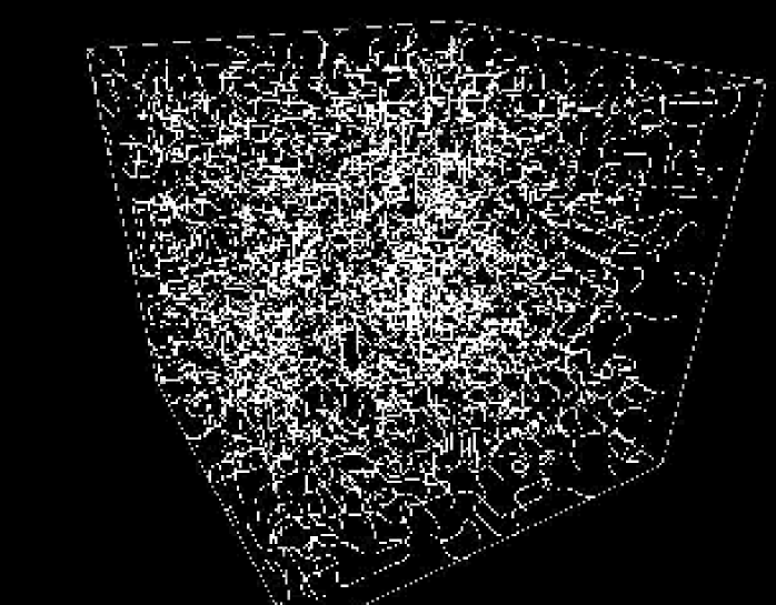
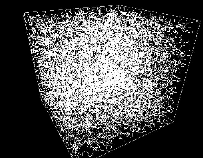
Figure 5.3: Configurations initiales d’un réseau de cordes, calculées par l’algorithme de Vachaspati et Vilenkin [335], dans un volume comobile de côté $16\ell_{\mathrm{c}}$ et $26\ell_{\mathrm{c}}$, respectivement. La distribution de cordes est constituée de $80\%$ de cordes infinies contre $20\%$ de boucles, indépendamment du volume de référence.

Les résultats numériques indiquent que le réseau de cordes formé par la transition de phase comprend $80\%$ de cordes infinies, dont la forme est typiquement celle d’une marche aléatoire [335], et $20\%$ de boucles de tailles caractéristiques $R$, dont la densité varie en $1/R^{4}$ indépendamment des autres paramètres physiques. Le calcul numérique de l’évolution de ce réseau nécessite maintenant la connaissance du mouvement de chaque corde dans FLRW, ainsi que la prise en compte des intercommutations.

Évolution dans FLRW

L’espace-temps de FLRW privilégiant le choix d’un référentiel comobile, le formalisme traditionnel y est particulièrement adapté pour la description des cordes. Comme dans le cas de l’espace-temps de Minkowski, l’action de Goto-Nambu permet d’obtenir les équations du mouvement (4.7), et les degrés de liberté inhérents au choix des systèmes de coordonnées peuvent être fixés par des choix de jauge. Dans le cas de FLRW, il pourrait sembler commode de se placer dans la jauge conforme (4.9), mais malheureusement ce choix de jauge n’est plus compatible avec le choix de jauge transverse (4.11), du fait des valeurs non nulles des symboles de Christoffel. On choisit alors les conditions de jauge mixtes

$$\xi^{0}=\eta,\quad\xi^{1}=\xi,\quad\dot{\vec{x}}^{\,\raisebox{-1.0pt}[0.0pt][0.0pt]{\tiny}}.\vec{x}^{\,{}^{\prime}\raisebox{2.2pt}[0.0pt][0.0pt]{\tiny}}=0,$$ (5.9)

avec $\eta$ le temps cosmique conforme [voir Eq. (1.8)], et $\dot{\vec{x}}^{\,\raisebox{-1.0pt}[0.0pt][0.0pt]{\tiny}}$ la vitesse conforme de la corde, qui est choisie purement transverse, comme cela est suggéré par l’invariance de Lorentz longitudinale (voir Sect. 4.2). L’équation du mouvement (4.7) se simplifie alors en

$$\ddot{\vec{x}}^{\,\raisebox{-1.0pt}[0.0pt][0.0pt]{\tiny}}+2{\mathcal{H}}\,\dot{\vec{x}}^{\,\raisebox{-1.0pt}[0.0pt][0.0pt]{\tiny}}\left(1-\dot{\vec{x}}^{\,\raisebox{-1.0pt}[0.0pt][0.0pt]{\tiny 2}}\right)=\frac{1}{\epsilon}\left(\frac{\vec{x}^{\,{}^{\prime}\raisebox{2.2pt}[0.0pt][0.0pt]{\tiny}}}{\epsilon}\right)^{\prime},$$ (5.10)

avec

$$\epsilon=\sqrt{\frac{\vec{x}^{\,{}^{\prime}\raisebox{2.2pt}[0.0pt][0.0pt]{\tiny 2}}}{1-\dot{\vec{x}}^{\,\raisebox{-1.0pt}[0.0pt][0.0pt]{\tiny 2}}}}.$$ (5.11)

Les condition de jauge (5.9) et l’équation du mouvement (5.10) imposent de plus

$$\frac{\dot{\epsilon}}{\epsilon}=-2{\mathcal{H}}\,\dot{\vec{x}}^{\,\raisebox{-1.0pt}[0.0pt][0.0pt]{\tiny 2}},$$ (5.12)

et à partir de (4.5), l’énergie totale d’une corde est directement donnée par $\epsilon$ [329]

$$M=aU\int\epsilon\,{\mathrm{d}}\xi.$$ (5.13)

Ses variations avec le temps conforme s’obtiennent en reportant (5.13) dans l’équation d’évolution (5.12). On trouve

$$\frac{\dot{M}}{M}={\mathcal{H}}\left(1-2\,\overline{v^{2}}\right),$$ (5.14)

où la vitesse quadratique moyenne $\overline{v^{2}}$ est définie par

$$\overline{v^{2}}=\frac{\displaystyle\int{\epsilon\,\dot{\vec{x}}^{\,\raisebox{-1.0pt}[0.0pt][0.0pt]{\tiny 2}}}{\mathrm{d}}\xi}{\displaystyle\int{\epsilon}\,{\mathrm{d}}\xi}.$$ (5.15)

D’après l’équation (5.14), l’énergie totale de la corde augmente donc proportionnellement au facteur d’échelle, comme intuitivement attendu (voir Sect. 5.3.1). Cependant, le terme en $\overline{v^{2}}$ tend à réduire ce gain d’énergie, voire même à l’annuler pour $\overline{v^{2}}=0.5$. En fait, comme le montre le terme de friction de l’équation (5.10), l’expansion de l’univers tend à atténuer les oscillations propres de la corde, et donc à réduire $\overline{v^{2}}$ sur des échelles de distance comparable à l’horizon. Inversement, aux petites échelles de longueur, cette atténuation sera négligeable et les oscillations propres des boucles vont certainement dominer la dynamique donnant $\dot{M}\simeq 0$, comme dans l’espace-temps de Minkowski.

La résolution numérique de l’équation (5.10) est un problème délicat à cause de la propagation des kinks apparaissant lors de chaque intercommutation (voir Sect. 5.2). Il est plus judicieux de transformer (5.10) en deux équations du premier ordre portant sur des variables indépendantes et constantes pour chaque kink. Ceci est réalisé en posant [31]

$$\vec{p}(\eta,u)=\frac{\vec{x}^{\,{}^{\prime}\raisebox{2.2pt}[0.0pt][0.0pt]{\tiny}}}{\epsilon}-\dot{\vec{x}}^{\,\raisebox{-1.0pt}[0.0pt][0.0pt]{\tiny}},\quad\vec{q}(\eta,v)=\frac{\vec{x}^{\,{}^{\prime}\raisebox{2.2pt}[0.0pt][0.0pt]{\tiny}}}{\epsilon}+\dot{\vec{x}}^{\,\raisebox{-1.0pt}[0.0pt][0.0pt]{\tiny}},$$ (5.16)

avec $\vec{p}^{{}^{\,2}}=\vec{q}^{{}^{\,2}}=1$ et $(u,v)$ un nouveau choix de coordonnée défini par

$$u\equiv\int{\epsilon}\,{\mathrm{d}}\xi-\eta,\quad v\equiv\int{\epsilon}\,{\mathrm{d}}\xi+\eta.$$ (5.17)

L’équation (5.10) devient, en fonction de ces nouveaux paramètres [31],

$$\dot{\vec{p}}^{\,\raisebox{-1.0pt}[0.0pt][0.0pt]{\tiny}} = {\mathcal{H}}\left[\vec{q}-\left(\vec{p}.\vec{q}\,\right)\vec{p}\,\right],$$ (5.18)

$$\dot{\vec{q}}^{\,\raisebox{-1.0pt}[0.0pt][0.0pt]{\tiny}} = {\mathcal{H}}\left[\vec{p}-\left(\vec{p}.\vec{q}\,\right)\vec{p}\,\right],$$ (5.19)

$$\dot{\epsilon} = -{\mathcal{H}}\,\epsilon\left(1-\vec{p}.\vec{q}\,\right).$$ (5.20)

Les kinks se propageant à la vitesse de la lumière le long des deux directions de la corde, ils correspondent à des valeurs de $u$ et $v$ constantes. Ainsi, sur la grille $(u,v)$, les valeurs de $\vec{p}$ et $\vec{q}$ correspondantes peuvent être choisies constantes le long de chaque segment, et seront plus ou moins discontinues en chaque point par la présence des kinks. Cependant, l’intercommutation nécessite également la connaissance, à chaque instant, des coordonnées physiques $\vec{x}$ sur la grille initiale $(\eta,\xi)$. Celles-ci sont obtenues en inversant les relations précédentes, et il vient

$$\dot{\vec{x}}^{\,\raisebox{-1.0pt}[0.0pt][0.0pt]{\tiny}}=\frac{1}{2}\left(\vec{q}-\vec{p}\,\right),\quad\vec{x}^{\,{}^{\prime}\raisebox{2.2pt}[0.0pt][0.0pt]{\tiny}}=\frac{1}{2}\epsilon\left(\vec{p}+\vec{q}\,\right).$$ (5.21)

Une fois connue la position physique des points de chaque corde, la détection des intercommutations est essentiellement réalisée en testant pour chaque segment de corde, si, dans une liste de segments voisins, le volume du tétrahèdre sous-tendu par les quatre points des deux segments change de signe durant le pas de temps élémentaire. Si c’est le cas, l’intercommutation est effectuée.

Résultats numériques

À partir des configurations initiales de la figure 5.3, il est enfin possible de calculer leur évolution en résolvant numériquement les équations (5.18) à (5.21), et en détectant toutes les intercommutations survenant au cour du temps. Les résultats présentés ici sont issus d’un code numérique développé en FORTRAN90 et OpenMP fonctionnant sur des machines multiprocesseurs à mémoire partagée (voir annexe 11). Il est construit sur la base d’un des meilleurs codes des années 1980, développé par Bennett et Bouchet [33, 31], ayant originellement confirmé l’existence de la solution d’échelle (5.8).

Sur la figure 5.4 sont représentées les courbes d’évolution de la densité d’énergie totale associée aux cordes plus grandes que l’horizon en fonction du temps conforme. Que ce soit dans l’ère de matière ou de radiation, celle-ci tend toujours, indépendamment des conditions initiales, vers la loi d’échelle (5.8) en $1/t^{2}$. Dans l’ère de matière, et de radiation, on obtient numériquement, respectivement

$$\rho_{\infty_{\mathrm{mat}}}\simeq 28\,\frac{U}{a^{2}\eta^{2}},\quad\rho_{\infty_{\mathrm{rad}}}\simeq 40\,\frac{U}{a^{2}\eta^{2}}.$$ (5.22)

Figure 5.4: Évolution de la densité d’énergie totale associée aux cordes infinies, i.e. plus grandes que l’horizon, en fonction du temps conforme, dans l’ère de radiation (en haut) et de matière. Dans les deux cas, la loi d’échelle en $1/t^{2}$ est un attracteur, quelques soient les conditions initiales. La plus longue simulation est réalisée sur un volume comobile de $(48\ell_{\mathrm{c}})^{3}$ et met en jeu $2500000$ points.

Les simulations numériques confirment ainsi le mécanisme d’évacuation d’énergie par formation des boucles. Sur la figure 5.5 est représentée l’évolution de la densité d’énergie des cordes infinies (voir Fig. 5.4) comparée à la densité d’énergie de toutes les cordes, incluant les boucles. La loi d’échelle n’est clairement vérifiée que pour les cordes plus grandes que l’horizon, elle ne peut donc être applicable au réseau que si l’énergie associée aux boucles est effectivement évacuée, par rayonnement gravitationnel par exemple. Cependant, comme on peut le voir sur la figure 5.6, la taille caractéristiques des boucles formées est extrêmement plus faible que l’échelle de longueur typique du réseau de cordes infinies $L_{\infty}$. Cette observation [33] montre donc qu’il existe une autre échelle de longueur caractérisant le réseau à petite échelle et qu’elle est de plus déterminante dans la nature des intercommutations formant les boucles. Cette longueur caractéristique est liée à l’existence des kinks apparaissant lors des intercommutations (voir Sect. 5.2). En effet, la persistance de ces discontinuités dans la forme des cordes donne une structure à petite échelle qui favorise de nouvelles intersections sur des longueurs de plus en plus petites, et de fait la formation privilégiée de boucles de petites tailles [33, 47, 31]. D’autre part, d’après l’équation (5.10), le terme d’amortissement dans la propagation des kinks dépend directement du taux d’expansion de l’univers, et celui-ci étant plus important dans l’ère de matière, le lissage de la structure induite par les kinks y est plus efficace que dans l’ère de radiation. En conséquence, les boucles produites dans l’ère de radiation devraient être plus petites que celles générées dans l’ère de matière. Ceci apparaît clairement sur la figure 5.6 si on compare la distribution des boucles sur les deux prises de vue obtenues lorsque le régime stationnaire des grandes cordes est atteint. La plus petite taille des boucles dans l’ère de radiation nécessite également leur plus grand nombre pour atteindre le régime stationnaire (voir Fig. 5.6).

Figure 5.5: Évolution de la densité d’énergie totale des cordes infinies dans l’ère de radiation, en trait plein noir, comparée à celle des boucles, en tirets rouges courts. La densité d’énergie totale du réseau, incluant les boucles et les cordes plus grandes que l’horizon, est représentée en tirets bleus longs. La solution d’échelle en $1/t^{2}$ n’est donc rendue possible que par la formation des boucles, et leur désintégration en une forme d’énergie ne dominant pas la dynamique de l’univers (en partique des ondes gravitationnelles).

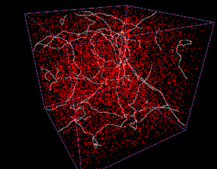
Figure 5.6: Configuration du réseau de cordes dans l’ère de matière (en haut) et de radiation, lorsque le régime stationnaire est atteint et lorsque le volume comobile initial est complètement contenu dans l’horizon. La structure à petite échelle des cordes est clairement visible dans leur forme et par la taille et le grand nombre de boucles (en rouge) générées au cour de l’évolution (la plupart sont en dessous de la résolution de l’image et apparaissent comme des points).

La loi d’échelle atteinte par les cordes infinies suggère que la densité d’énergie associée aux boucles, lorsque l’on considère cette fois leur désintégration par rayonnement gravitationnel, doit également atteindre une loi d’échelle [33]. La longueur moyenne $L_{\mathrm{b}}$ des boucles dans ce régime stationnaire reste alors une fraction constante de la distance à l’horizon

$$L_{\mathrm{b}}=\alpha t.$$ (5.23)

Les simulations numériques ne donnent cependant qu’une valeur maximale au coefficient de proportionnalité, $\alpha<10^{-3}$ dans le cas du code utilisé ici [33, 31]. Il existe néanmoins une limite inférieure qui est donnée par l’échelle de distance associée au rayonnement gravitationnel $\alpha>\gamma_{\mathrm{g}}{\mathcal{G}}U$ [voir Eq. (4.22)]. Il est possible de montrer, à l’aide des modèles effectifs [209, 32, 341], que la densité d’énergie totale des boucles rayonnantes suit la loi d’échelle

$$\rho_{{\mathrm{b}}_{\mathrm{rad}}}\simeq\sqrt{\frac{\alpha}{\gamma_{\mathrm{g}}{\mathcal{G}}U}}\rho_{\infty_{\mathrm{rad}}},$$ (5.24)

dans l’ère de radiation, et

$$\rho_{{\mathrm{b}}_{\mathrm{mat}}}\simeq 0.4\sqrt{\alpha}\ln\left(\frac{\alpha}{\gamma_{\mathrm{g}}{\mathcal{G}}U}\right)\rho_{\infty_{\mathrm{mat}}},$$ (5.25)

dans l’ère de matière. En supposant que la majeure partie de l’énergie gravitationnelle émise par le réseau l’est par les boucles, il est possible d’en estimer son intensité. Il est d’usage de considérer le paramètre de densité d’énergie gravitationnelle par unité logarithmique de fréquence [339, 183]

$$\Omega_{\mathrm{g}}=\frac{1}{\rho_{\mathrm{c}}}\nu\frac{{\mathrm{d}}\rho_{\mathrm{g}}}{{\mathrm{d}}\nu},$$ (5.26)

où $\rho_{\mathrm{g}}$ est la densité d’énergie sous forme d’ondes gravitationnelles de fréquence $\nu$, et $\rho_{\mathrm{c}}$ la densité critique. Comme dans la section 4.2, ce paramètre peut grossièrement être estimé en ne considérant que la fréquence caractéristique des boucles, i.e. $\nu\simeq 1/L_{\mathrm{b}}$. L’énergie gravitationnelle émise au temps $t_{\mathrm{e}}$ s’identifie à la densité totale d’énergie des boucles qui se sont désintégrées jusque là, i.e. les boucles qui avaient une longueur $L_{\mathrm{b}}\simeq\alpha t_{\mathrm{e}}$ aux temps antérieurs [voir Eq. (4.22)]. Il vient alors, d’après les équations (1.21), (5.22), (5.24) et (5.26)

$$\Omega_{\mathrm{g}}\simeq 100\sqrt{\frac{\alpha{\mathcal{G}}U}{\gamma_{\mathrm{g}}}}.$$ (5.27)

La connaissance des paramètres $\alpha$ et $\gamma_{\mathrm{g}}$ permet donc d’estimer la contribution d’un réseau de corde au fond d’ondes gravitationnelles existant dans l’univers en fonction de l’échelle de brisure de symétrie l’ayant générée $U$ [voir Eq. (5.27)]. Ce fond d’ondes gravitationnelles est cependant contraint par les prédictions de la nucléosynthèse primordiale [269, 164, 104, 29], et les mesures de régularité des temps de réception des signaux radios émis par les pulsars [46, 322]. En effet, dans le premier cas, il existe une densité d’énergie maximale des ondes gravitationnelles au delà de laquelle l’abondance des éléments légers prédite ne seraient plus compatible avec les observations (voir Fig. 1.4). Dans le deuxième cas, la modification de la géométrie de l’espace-temps nous séparant d’un pulsar, par le passage d’ondes gravitationnelles, devrait induire des variations dans les temps d’arrivée de ses signaux. L’absence de ces irrégularités actuellement observée donne donc également une limite supérieure au fond d’ondes gravitationnelles. À l’aide des simulations numériques et de ces deux contraintes observationnelles, on peut montrer que [46, 29]

$${\mathcal{G}}U\lesssim 10^{-6}.$$ (5.28)

Un telle contrainte sur l’échelle de brisure de symétrie n’est pas en faveur de la formation d’un réseau de cordes de Goto-Nambu aux échelles d’énergie de grande unification, et exclue quasiment leur origine dans les mécanismes de formation des grandes structures [47, 29, 11, 27, 98, 12].

5.3.3 Influence sur le CMBR

Les simulations numériques permettent également de calculer les déformations subies par une onde plane électromagnétique traversant le réseau de cordes par l’effet Kaiser-Stebbins (voir Sect. 3.3.3). Appliqués au rayonnement fossile, ces résultats permettent de dresser des cartes de température du CMBR où les anisotropies sont générées uniquement par les cordes cosmiques [47] (voir Sect. 3.4). Il est alors possible d’en déduire la valeur moyenne des fluctuations de température du CMBR créées par ces cordes[47]

$$\overline{\left(\frac{\delta\Theta}{\Theta}\right)}_{2}\simeq 19\,{\mathcal{G}}U.$$ (5.29)

L’observation de fluctuations de température de l’ordre de $10^{-5}$ (voir Figs. 1.3 et 3.8) donne une condition sur l’échelle de brisure de symétrie formant le réseau de corde du même ordre de grandeur que (5.28). Cependant, dans la section 3.4, nous avons vu que le spectre de puissance du CMBR actuellement observé ne semblait pas être uniquement généré par des défauts topologiques, et bien que donnant toujours une limite supérieure à ${\mathcal{G}}U$, les résultats prédis par les cartes de température sont difficilement comparables aux observations.

Une autre approche consiste à ne s’intéresser qu’au spectre de puissance du CMBR afin d’y rechercher la signature éventuelle d’un réseau de cordes cosmiques. Dans la section 3.4, les résultats présentés sur la figure 3.9 ont été obtenus par superposition linéaire des spectres de puissance génériques associés aux défauts globaux seuls et à l’inflation seule [48]. Cette hypothèse est la plus simple que l’on puisse faire mais ne tient pas compte des effets de couplage entre les perturbations générées pas des défauts et les autres espèces présentes dans le plasma primordial. La proportion de défauts trouvée avoisinant les $20\%$ justifie une investigation plus poussée par des méthodes plus précises.

Le calcul théorique des anisotropies de température du CMBR passe par la détermination de l’évolution cosmologique des perturbations associées à la géométrie et à la matière qui sont susceptibles d’en modifier les caractéristiques physiques. Celles-ci sont généralement obtenues, dans l’approximation linéaire, à partir de la connaissance des perturbations $h_{\mu\nu}$ de la métrique (1.6) [230, 231, 298, 333]

$${\mathrm{d}}s^{2}=\left(g_{\mu\nu}+a^{2}h_{\mu\nu}\right){\mathrm{d}}x^{\mu}{\mathrm{d}}x^{\nu},$$ (5.30)

et de la description, hydrodynamique ou particulaire, des perturbations associées aux différents fluides présents dans l’univers primordial. Les équations d’évolution sont alors données par les équations d’Einstein (1.13) appliquées aux quantités perturbées

$$\widetilde{G}^{\mu\nu}=\kappa^{2}\widetilde{T}_{\mathrm{tot}}^{\mu\nu},$$ (5.31)

où $\widetilde{G}^{\mu\nu}$ est le tenseur d’Einstein perturbé obtenu à partir de la métrique (5.30), et $\widetilde{T}^{\mu\nu}_{\mathrm{tot}}$ le tenseur énergie-impulsion total associé au diverses sources d’anisotropies. Celui-ci dépend intrinsèquement des propriétés et des interactions des divers fluides présents. L’influence de l’existence d’un réseau de cordes cosmiques peut être prise en compte dans le terme source $\widetilde{T}^{\mu\nu}_{\mathrm{tot}}$, une fois sa contribution $T^{\mu\nu}_{\mathrm{s}}$ connu. En fait, puisque l’on s’intéresse uniquement à la statistique des fluctuations au travers des fonctions de corrélations (voir Sect. 3.4), les quantités à déterminer seront les corrélateurs à deux points du tenseur énergie-impulsion du réseau

$$C^{\mu\nu\rho\sigma}=\langle T^{\mu\nu}_{\mathrm{s}}(\eta,\vec{x}\,)\,T^{\rho\sigma}_{\mathrm{s}}(\eta^{\prime},\vec{x}^{\,{}^{\prime}\raisebox{2.2pt}[0.0pt][0.0pt]{\tiny}})\rangle,$$ (5.32)

où la valeur moyenne porte sur l’ensemble des différentes réalisations de la transition de phase. La résolution des équations (5.31), pour les corrélateurs, est actuellement réalisée par différents codes numériques [298] nécessitant en entrée la connaissance des corrélateurs des tenseurs énergie-impulsion des sources. L’intérêt des simulations numériques de cordes est aujourd’hui de permettre une détermination de leur corrélateurs $C^{\mu\nu\rho\sigma}$ afin d’inclure leurs effets au sein de la dynamique des perturbations cosmologiques. À partir des équations (1.6), (4.5) et (5.9), le tenseur énergie-impulsion d’une corde dans FLRW se réduit à

$$\sqrt{-g}\,T^{\mu\nu}(\eta,\vec{r}\,)=U\int{{\mathrm{d}}\xi}\left(\epsilon\,\dot{x}^{\mu}\dot{x}^{\nu}-\frac{1}{\epsilon}x^{\prime\mu}x^{\prime\nu}\right)\delta^{3}\left[\vec{r}-\vec{x}(\eta,\xi)\right],$$ (5.33)

avec $\epsilon$ donné par (5.11), dans la jauge mixte (5.9). Sa détermination est particulièrement adaptée à la méthode numérique du code utilisé ici, en effet, en reportant l’équation (5.21) dans l’expression précédente, il vient

$$\sqrt{-g}\,T^{\mu\nu}(\eta,\vec{r}\,)=-U\int{\epsilon\,{\mathrm{d}}\xi}\,\frac{1}{2}\left(p^{\mu}q^{\nu}+q^{\mu}p^{\nu}\right)\delta^{3}\left[\vec{r}-\vec{x}(\eta,\xi)\right].$$ (5.34)

Le volume comobile de référence (voir Fig. 5.4) peut être discrétisé afin de calculer, dans chaque cellule centrée sur $\vec{r}$, la valeur totale, au temps $\eta$, du tenseur énergie-impulsion des cordes qu’elle contient. On obtient ainsi un ensemble de valeurs $T^{\mu\nu}_{\mathrm{s}}(\eta,\vec{r}\,)$ pour le réseau de corde, dont les corrélateurs sont donnés, dans l’espace de Fourier, par

$$\widehat{C}^{\mu\nu\rho\sigma}(\eta,\eta^{\prime},\vec{k}\,)=\widehat{T}^{\mu\nu}_{\mathrm{s}}(\eta,-\vec{k}\,)\,\widehat{T}^{\rho\sigma}_{\mathrm{s}}(\eta^{\prime},\vec{k}^{\,{}^{\prime}\raisebox{2.2pt}[0.0pt][0.0pt]{\tiny}}),$$ (5.35)

où la transformée de Fourier est définie par

$$\widehat{C}(\vec{k}\,)=\int{{\mathrm{d}}^{3}\vec{r}}\,C(\vec{r}\,){\mathrm{e}}^{i\vec{k}.\vec{r}},$$ (5.36)

et où l’on a utilisé, pour les fonctions réelles $T^{\mu\nu}_{\mathrm{s}}(\eta,\vec{r})$, la relation

$$\left[\widehat{T}^{\mu\nu}_{\mathrm{s}}(\eta,\vec{k}\,)\right]^{\dagger}=\widehat{T}^{\mu\nu}_{\mathrm{s}}(\eta,-\vec{k}\,).$$ (5.37)

La moyenne statistique des corrélateurs (5.35) peut être effectuée sur différentes simulations numériques obtenues par différents choix de conditions initiales. En collaboration avec A. Riazuelo, auteur d’un code Boltzmann d’évolution de perturbations cosmologiques [273, 298], le calcul du spectre de puissance correspondant est actuellement en cours. Nous pourrons donc, d’ici peu, statuer précisément sur la proportion de cordes cosmiques locales dans les observations du CMBR.

5.4 Conclusion

Les simulations numériques montrent l’importance du mécanisme de formation de boucles dans l’évolution cosmologique des réseaux de cordes par la désintégration nécessaire de celles-ci en une forme d’énergie ne dominant pas l’univers (voir Fig. 5.5). Sous ces conditions, l’existence d’un réseau est compatible avec les observations pour des échelles d’énergie de brisure de symétrie inférieures à celles de grande unification, i.e. ${\mathcal{G}}U<10^{-6}$. Il est également possible qu’une contribution non négligeable de ces cordes soit actuellement détectable dans les données du CMBR, et dont la signature pourra être d’ici peu vérifiée ou infirmée grâce aux simulations numériques.

Cependant, comme on l’a vu par les formalismes macroscopiques (voir Chap. 4), il existe des types de corde pour lesquelles les boucles formées peuvent être stables. Ce sont celles possédant une structure interne générée par un courant de particules. Il n’existe pas, à l’heure actuelle, de code numérique permettant d’en calculer l’évolution cosmologique, mais comme l’approche qualitative de la section 5.3.1 le suggère, la loi d’échelle atteinte par les réseaux au cours de leur évolution semble robuste, et le même mécanisme appliqué à ces cordes devrait produire une grande proportion de boucles conductrices potentiellement stables, aboutissant ainsi à leur domination sur les autres formes d’énergie. Un tel scénario n’est pas compatible avec les observations, et comme nous le verrons dans les sections suivantes, la présence de courants sur les cordes semble en être une propriété générique. La stabilité des boucles (voir Sect. 4.3.4) devient donc un critère cosmologique d’existence de ces cordes, et de ce fait, une contrainte sur les symétries effectivement brisées dans l’univers primordial.

Chapitre 6 Génération de courants sur les cordes

6.1 Introduction

Les chapitres précédents ont mis en évidence l’importance cosmologique des boucles de corde cosmique. Leur conversion en une forme d’énergie ne dominant pas l’univers est une condition nécessaire à l’existence d’un réseau dans l’univers. Cependant, dans le chapitre 4, le formalisme covariant nous a permis de montrer que la brisure de l’invariance de Lorentz longitudinale par un courant conservé le long des cordes pouvait stabiliser les boucles. Il est, de ce fait, légitime de s’interroger sur l’existence et la pertinence de mécanismes microphysiques pouvant être à l’origine de ces courants. Dans le cadre du modèle de Higgs abélien, il est possible de coupler la théorie microphysique, décrivant de purs vortex, à d’autres champs pouvant éventuellement se propager le long de la corde. Le cas le plus simple est celui d’un champ scalaire additionnel couplé au champ de Higgs. E. Witten a en effet montré qu’un condensât de ce champ peut se former au centre du vortex et générer un courant de particules scalaires [362]. Les équations du mouvement de ces cordes supraconductrices sont plus compliquées du fait de la présence de champs supplémentaires, il en résulte que la description analytique de leurs propriétés dynamiques est difficile. C’est pourquoi le formalisme covariant est habituellement préféré: la simple connaissance de l’équation d’état fixe la dynamique des cordes et la stabilité des boucles associées (voir Chap. 4). La correspondance entre l’approche microscopique et le formalisme covariant s’effectue naturellement par le passage à la limite d’épaisseur nulle de la théorie quadri-dimensionnelle. P. Peter a obtenu, de cette manière, l’équation d’état des cordes possédant un condensât de Bose [282, 281]. Ce lien est indispensable car il permet d’une part, de justifier l’emploi de l’approche macroscopique pour des cordes possédant une structure interne, et d’autre part, d’exprimer les grandeurs macroscopiques, telle l’énergie par unité de longueur ou la tension, en fonction des paramètres microscopiques de la physique des particules sous-jacente. Ces paramètres peuvent ainsi être fixés par les contraintes cosmologiques directement déduites du formalisme covariant.

6.2 Le modèle de Witten scalaire

À partir du modèle de Higgs abélien (2.29) décrivant la microphysique d’une corde de Goto-Nambu, il est possible de coupler un champ scalaire $\Sigma$ supplémentaire au champ de Higgs $\Phi$ formant la corde. Par analogie avec la supraconductivité dans les matériaux, l’idée est de briser une symétrie additionnelle uniquement au centre du vortex afin que le champ $\Sigma$ puisse s’y condenser. Le cas le plus simple est celui d’une invariance $U_{\mathrm{b}}(1)$, qui peut être choisie locale ou globale selon que le champ scalaire $\Sigma$ est chargé ou non, respectivement. La forme générale du lagrangien associé au champ $\Sigma$ s’écrit, dans le cas d’une symétrie $U_{\mathrm{b}}(1)$ locale, d’après (2.13)

$${\mathcal{L}}_{\Sigma}=\frac{1}{2}\left(\widetilde{D}_{\mu}\Sigma\right)^{\dagger}\left(\widetilde{D}^{\mu}\Sigma\right)-\frac{1}{4}N_{\mu\nu}N^{\mu\nu}-\frac{\widetilde{\lambda}}{8}|\Sigma|^{4}-\frac{1}{2}m_{\sigma}^{2}|\Sigma|^{2}$$ (6.1)

où $N^{\mu\nu}$ est le tenseur de type Faraday associé au champ de jauge $C^{\mu}$ de la symétrie $U_{\mathrm{b}}(1)$, et

$$\widetilde{D}_{\mu}=\partial_{\mu}+i\,\widetilde{g}\,C_{\mu},$$ (6.2)

la dérivée covariante associée. Cette symétrie de jauge peut, par ailleurs, être identifiée à l’électromagnétisme. L’interaction de $\Sigma$ avec le champ de Higgs formant la corde s’écrit, de manière générale,

$${\mathcal{L}}_{\mathrm{int}}=f\left(\eta^{2}-|\Phi|^{2}\right)|\Sigma|^{2},$$ (6.3)

où $f$ est la constante de couplage entre les deux champs, et $f\eta^{2}$ un terme de masse additionnel qui peut être absorbé dans $m_{\sigma}^{2}$. L’intérêt d’avoir écrit le lagrangien d’interaction sous la forme (6.3) est que loin de la corde, si le champ de Higgs $\Phi$ prend sa valeur moyenne dans le vide $|\Phi|=\eta$, la masse physique du boson $\Sigma$ est donnée par $m_{\sigma}$. Le potentiel total associé à $\Phi$ s’écrivant, d’après (2.29), (2.32) et (6.3),

$$V_{\mathrm{tot}}(\Phi)=\frac{\lambda}{8}\left(|\Phi|^{2}-\eta^{2}\right)^{2}+f|\Sigma|^{2}|\Phi|^{2},$$ (6.4)

il est effectivement minimisé en $|\Phi|=\eta$ et $|\Sigma|=0$. Inversement, au centre de la corde $\Phi=0$ et, pourvu que $f\eta^{2}>m_{\sigma}^{2}/2$, le champ $\Sigma$ semble acquérir une masse négative caractéristique de la brisure de la symétrie $U_{\mathrm{b}}(1)$ (voir Sect. 2.3). En effet, le potentiel du champ $\Sigma$ au centre de la corde est, d’après les équations (6.1) et (6.3),

$$\left.\widetilde{V}(\Sigma)\right|_{\Phi=0}=\frac{\widetilde{\lambda}}{8}|\Sigma|^{4}+\frac{1}{2}\left(m_{\sigma}^{2}-2f\eta^{2}\right)|\Sigma|^{2},$$ (6.5)

Dans le cas où $f\eta^{2}<m_{\sigma}^{2}/2$, ce potentiel est minimisé pour $|\Sigma|=0$ et la symétrie $U_{\mathrm{b}}(1)$ n’est pas brisée, alors que si $f\eta^{2}>m_{\sigma}^{2}/2$, il est minimisé pour

$$|\Sigma|=2\sqrt{\frac{2f\eta^{2}-m_{\sigma}^{2}}{\widetilde{\lambda}}}.$$ (6.6)

On obtient, dans ce dernier cas, un condensât du champ au centre de la corde où la symétrie $U_{\mathrm{b}}(1)$ est brisée. Par continuité, le champ $\Sigma$ va rejoindre son état de vide $\Sigma=0$ loin de la corde, et par symétrie cylindrique, va être uniquement une fonction de la distance au vortex que nous noterons $\Sigma_{{}_{0}}(r)$. Notons que le lagrangien (6.1) peut également conduire à la formation de cordes cosmiques par la brisure spontannée de la symétrie $U_{\mathrm{b}}(1)$ lors du refroidissement de l’univers. Ceci peut être évité en choisissant les paramètres physiques associés à $\Sigma$ tels que sa température de transition de phase soit bien inférieure à celle de $\Phi$, i.e. d’après (3.39) $m_{\sigma}/\widetilde{\lambda}^{1/2}<\eta$.

D’après (6.6), l’ensemble des valeurs du champ $\Sigma$ de la forme

$$\Sigma=|\Sigma_{{}_{0}}|{\mathrm{e}}^{i\psi(\xi^{a})},$$ (6.7)

avec $\psi(\xi^{a})$ une fonction réelle des coordonnées longitudinales, minimisent également le potentiel dans le vortex. Par le théorème de Noether, l’invariance $U_{\mathrm{b}}(1)$ de la théorie impose au courant $j^{\mu}=\delta{\mathcal{L}}_{\Sigma}/\delta C_{\mu}$ d’être conservé. Ses composantes le long de la corde s’obtiennent à partir de (6.1) et (6.7), et on trouve

$$j^{a}=\widetilde{g}\,|\Sigma_{{}_{0}}|^{2}\left(\partial^{a}\psi+\widetilde{g}\,C^{a}\right).$$ (6.8)

La persistance de ce courant est assurée pour des raisons topologiques similaires à celles assurant l’existence des cordes: le long d’une boucle de corde, la phase $\psi$ ne peut varier que d’un multiple entier de $2\pi$ permettant de définir un invariant topologique [362, 341]

$$N=\frac{1}{2\pi}\oint{{\mathrm{d}}\xi}\,\frac{{\mathrm{d}}\psi}{{\mathrm{d}}\xi},$$ (6.9)

avec $\xi$ l’abscisse curviligne. Ce courant peut être estimé en calculant le potentiel vecteur $C^{a}$. Dans la jauge de Coulomb, i.e. $\partial_{i}C^{i}=0$, la solution des équations (2.1) est donnée par

$$C^{a}(\vec{r}\,)=-\frac{1}{4\pi}\oint{{\mathrm{d}}\xi}\,\frac{j^{a}\left[\vec{x}(\xi)\right]}{\left|\vec{r}-\vec{x}(\xi)\right|},$$ (6.10)

avec $\vec{x}(\xi)$ la position de la corde dans un référentiel privilégié. D’après (6.10), le potentiel vecteur diverge logarithmiquement avec la distance près du centre du vortex. La largeur de la corde étant, en première approximation, donnée par l’inverse de la masse du Higgs (voir Sect. 3.3), un ordre de grandeur de la partie divergente de (6.10) est $-\ln\left(m_{\mathrm{h}}L_{\mathrm{b}}\right)$, avec $L_{\mathrm{b}}$ la longueur de la boucle. Il vient finalement

$$C^{a}\simeq-\ln\left(m_{\mathrm{h}}L_{\mathrm{b}}\right)j^{a},$$ (6.11)

qui, combiné avec les équations (6.8) et (6.9), donne la composante spatiale du courant le long de la corde

$$j^{z}\simeq\frac{\widetilde{g}\,|\Sigma_{{}_{0}}|^{2}}{1+\widetilde{g}^{2}|\Sigma_{{}_{0}}|^{2}\ln\left(m_{\mathrm{h}}L_{\mathrm{b}}\right)}\,\frac{N}{L_{\mathrm{b}}}\simeq\frac{1}{\widetilde{g}\ln\left(m_{\mathrm{h}}L_{\mathrm{b}}\right)}\,\frac{N}{L_{\mathrm{b}}}.$$ (6.12)

Bien que son amplitude soit directement reliée à la charge topologique $N$, le courant $j^{z}$ est limité physiquement par l’existence du condensât sur la corde, c’est-à-dire qu’il est nécessaire que l’état excité du condensât reste l’état d’énergie minimale. Or, dès que le courant est présent, pour $N\neq 0$, le terme cinétique du lagrangien (6.1) peut se voir comme une contribution négative à un potentiel effectif pour $\Sigma$ dont la composante spatiale est de l’ordre de

$$\left(\widetilde{D}_{z}\Sigma\right)^{\dagger}\left(\widetilde{D}_{z}\Sigma\right)=-|\Sigma_{{}_{0}}|^{2}\left(N+\widetilde{g}\,C_{z}\right)^{2}.$$ (6.13)

La brisure de la symétrie $U_{\mathrm{b}}(1)$ n’est encore assurée au centre de la corde, d’après (6.1) et (6.5), que pour

$$\left(N+\widetilde{g}\,C_{z}\right)^{2}<f\eta^{2}-\frac{1}{2}m_{\sigma}^{2},$$ (6.14)

soit, à l’aide de (6.11) et (6.12),

$$N^{2}<\left(\frac{L_{\mathrm{b}}}{L_{\mathrm{b}}+1}\right)^{2}\left(f\eta^{2}-\frac{1}{2}m_{\sigma}^{2}\right).$$ (6.15)

Il y a donc un courant maximal au delà duquel il est énergétiquement préférable aux particules se propageant le long de la corde de rejoindre leur état de vide usuel $\Sigma=0$.

Le modèle de Witten conduit, par le couplage le plus simple qu’un champ scalaire additionnel puisse avoir avec le champ de Higgs, à la naissance d’un courant conservé le long de la corde. Il est clair que la dynamique de celle-ci, ainsi que la stabilité des boucles associées, vont en être modifiées. Notons que le courant (6.12) introduit seulement un paramètre physique supplémentaire, $\psi$, par rapport au cas de Goto-Nambu, lorsque l’on passe à la limite d’épaisseur nulle. Il est donc raisonnable d’espérer décrire la dynamique macroscopique d’une telle corde par le formalisme covariant introduit au chapitre 4.

6.3 Correspondance avec le formalisme covariant

L’approche microscopique précédente permet la détermination, par le passage à la limite d’épaisseur nulle, des quantités macroscopiques nécessaires à la description d’une corde conductrice dans le formalisme covariant, c’est-à-dire l’énergie par unité de longueur et la tension, ainsi que le paramètre d’état $\varpi$ tenant compte de l’influence du courant. Afin de ne pas perdre complètement l’information concernant la structure transverse du vortex, la connaissance de la dynamique des champs en interaction est indispensable avant de pouvoir la moyenner sur les dimensions transverses à la corde. Comme c’était le cas pour le modèle de Higgs abélien (voir Sect. 3.3.1), la résolution des équations du mouvement, dans le modèle de Witten, nécessite l’emploi de méthodes numériques [23, 282, 281]. En utilisant des méthodes de relaxation [6], P. Peter a, de cette manière, confirmé la validité du formalisme covariant pour ces types de corde tout en dérivant la forme exacte de l’équation d’état.

Les équations d’Euler-Lagrange des différents champs obtenues à partir du lagrangien du modèle de Witten scalaire,

$${\mathcal{L}}_{{\mathrm{w}}{\mathrm{b}}}={\mathcal{L}}_{\mathrm{h}}+{\mathcal{L}}_{\Sigma}+{\mathcal{L}}_{\mathrm{int}},$$ (6.16)

peuvent s’écrire, sous leur forme adimensionnée [281],

$$\left\{\begin{array}[]{lcl}\displaystyle\frac{{\mathrm{d}}H}{{\mathrm{d}}\varrho^{2}}+\frac{1}{\varrho}\frac{{\mathrm{d}}H}{{\mathrm{d}}\varrho}&=&\displaystyle\frac{1}{\varrho^{2}}HQ^{2}+\frac{1}{2}H(H^{2}-1)+2\frac{f\eta^{2}}{m_{\mathrm{h}}^{2}}\frac{m_{\sigma}^{2}}{m_{\times}^{2}}HS^{2},\\ \\ \displaystyle\frac{{\mathrm{d}}S}{{\mathrm{d}}\varrho^{2}}+\frac{1}{\varrho}\frac{{\mathrm{d}}S}{{\mathrm{d}}\varrho}&=&\displaystyle w\frac{m_{\times}^{2}}{m_{\sigma}^{2}}P^{2}S+2\frac{f\eta^{2}}{m_{\mathrm{h}}^{2}}(H^{2}-1)S+\frac{m_{\sigma}^{2}}{m_{\mathrm{h}}^{2}}S(S^{2}+1),\\ \\ \displaystyle\frac{{\mathrm{d}}Q}{{\mathrm{d}}\varrho^{2}}-\frac{1}{\varrho}\frac{{\mathrm{d}}Q}{{\mathrm{d}}\varrho}&=&\displaystyle\frac{m_{\mathrm{b}}^{2}}{m_{\mathrm{h}}^{2}}H^{2}Q,\\ \\ \displaystyle\frac{{\mathrm{d}}P}{{\mathrm{d}}\varrho^{2}}+\frac{1}{\varrho}\frac{{\mathrm{d}}P}{{\mathrm{d}}\varrho}&=&\displaystyle\frac{m_{\sigma}^{2}}{m_{\mathrm{h}}^{2}}\frac{m_{\mathrm{c}}^{2}}{m_{\times}^{2}}S^{2}P,\end{array}\right.$$ (6.17)

où l’on a introduit les paramètres

$$m_{\times}=\sqrt{\widetilde{\lambda}}\,\eta,\quad m_{\mathrm{c}}=\widetilde{g}\,\eta,$$ (6.18)

par analogie avec les paramètres donnant la masse du boson de Higgs $\Phi$ et du boson vecteur $B^{\mu}$ de la corde

$$m_{\mathrm{h}}=\sqrt{\lambda}\,\eta,\quad m_{\mathrm{b}}=g\,\eta.$$ (6.19)

Le champ de Higgs adimensionné $H$ et la composante orthoradiale du champ de jauge de la corde $Q$, ainsi que la variable transverse $\varrho$ sont donnés par les équations (3.41) à (3.44). Le champ scalaire $S$ est défini par

$$S=\frac{m_{\times}}{m_{\sigma}}\frac{|\Sigma_{{}_{0}}|}{\eta}.$$ (6.20)

Quant au potentiel vecteur $C^{\mu}$, associée à la symétrie $U_{\mathrm{b}}(1)$, et la phase $\psi$ à l’origine du courant topologique, ils permettent de définir le bivecteur $P^{a}$ par la relation

$$P_{a}\equiv\partial_{a}\psi+\widetilde{g}\,C_{a}.$$ (6.21)

Seule la norme adimensionnée $P$ de celui-ci intervient dans les équations de champs (6.17). Elle permet en outre de définir la quantité $\varpi$ qui s’identifie au paramètre d’état du formalisme covariant (voir Sect. 4.3.3):

$$P_{t}^{2}-P_{z}^{2}=\varpi P^{2}.$$ (6.22)

Le paramètre $\varpi$ apparaît également dans les équations du mouvement (6.17) sous sa forme adimensionnée

$$w=\frac{m_{\sigma}^{2}}{m_{\mathrm{h}}^{2}m_{\times}^{2}}\varpi.$$ (6.23)

Figure 6.1: Profils transverses des champs dans une corde cosmique de Witten possédant un condensât de Bose en son cœur [281]. Le champ de Higgs $H$ et le champ de jauge formant la corde $Q$ ont les mêmes caractéristiques que ceux formant une corde de Goto-Nambu (voir Fig. 3.3). Le champ scalaire $S$ se condense au centre du vortex, générant un courant dont la divergence logarithmique du champ de jauge $P$ associé est caractéristique d’un fil conducteur.

À partir de la résolution des équations (6.17) (voir Fig. 6.1) en fonction du paramètre $w$, la connaissance des variations transverses des champs permet de calculer le tenseur énergie impulsion $T^{ab}$, le long de la corde, à l’aide de l’équation (3.4) appliquée au lagrangien (6.16). Le courant topologique $j^{a}$ est pour sa part directement donné par (6.8). Leur valeurs bidimensionnelles, ${\overline{T}}^{ab}$ et ${\overline{j}}^{a}$, dans la limite d’épaisseur nulle, sont ensuite obtenues par intégration sur les directions transverses [79, 282, 281] (voir Sect. 3.3.1). L’énergie par unité de longueur $U$ et la tension $T$ sont finalement données, d’après la section 4.3, par

$$U={\overline{T}}^{tt},\quad T=-{\overline{T}}^{zz},$$ (6.24)

et l’intensité ${\mathcal{C}}$ du courant par

$${\mathcal{C}}=\sqrt{\left|{\overline{j}}_{t}^{2}-{\overline{j}}_{z}^{2}\right|}=2\pi\eta^{2}\frac{m_{\sigma}}{m_{\mathrm{h}}m_{\times}}\sqrt{|w|}\int{\varrho\,{\mathrm{d}}\varrho}\,S^{2}P.$$ (6.25)

On peut vérifier que ces grandeurs satisfont l’équation barotropique attendue par le formalisme covariant

$$U-T=\sqrt{|\varpi|}\,{\mathcal{C}}.$$ (6.26)

Sur la figure 6.2 sont représentées les variations de l’intensité du courant ${\mathcal{C}}$ en fonction du paramètre $-w/\sqrt{|w|}$ dont le signe, positif ou négatif, dépend maintenant du type de régime, magnétique ou électrique, respectivement (voir Sect. 4.3). Comme attendu par les considérations analytiques de la section précédente, on observe clairement une saturation du courant pour $|\varpi|\simeq m_{\sigma}^{2}$, dans le régime magnétique. Pour un paramètre d’état supérieur à cette valeur, l’intensité du courant diminue car l’état de condensation le long de la corde n’est plus énergétiquement favorisé, la fuite de particules scalaires vers l’état de vide usuel est privilégiée. De la même manière, dans le régime électrique, ${\mathcal{C}}$ représente cette fois la densité de particules condensées sur la corde, et, pour des valeurs du paramètre d’état $|\varpi|\rightarrow m_{\sigma}^{2}$, on observe une divergence de ${\mathcal{C}}$ appelée seuil de fréquence. L’interprétation physique en est similaire: l’énergie moyenne de chaque particule devient supérieure à leur masse $m_{\sigma}$ loin de la corde, et il n’existe plus de solution stationnaire aux équations de champ (6.17), ce qui se traduit par la divergence observée des solutions statiques sur la figure 6.2.

Figure 6.2: L’intensité du courant ${\mathcal{C}}$ en fonction du paramètre adimensionné $-w/\sqrt{|w|}$. Le condensât de Bose au centre du vortex n’est énergétiquement privilégié que pour $|\varpi|<m_{\sigma}^{2}$, au delà, les particules scalaires rejoignent leur état de vide loin de la corde entraînant une saturation du courant dans le régime magnétique, et un seuil de fréquence, caractérisé par la divergence de ${\mathcal{C}}$, dans le régime électrique [282]. La courbe en trait plein correspond à la limite $\widetilde{g}\rightarrow 0$ du modèle de Witten (c’est la limite neutre dans le cas où la symétrie $U_{\mathrm{b}}(1)$ représente l’électromagnétisme) et s’éloigne relativement peu de la courbe incluant le couplage au champ de jauge $C^{\mu}$: les propriétés physiques dominantes résultent principalement des effets mécaniques du courant le long de la corde, comme attendu par le formalisme covariant [79, 69].

Figure 6.3: L’énergie par unité de longueur $U$ et la tension $T$ d’une corde cosmique, parcourue par un courant de particules scalaires, en fonction du paramètre d’état. Comme sur la figure 6.2, les courbes en traits pleins et pointillés correspondent au condensât de Bose obtenu par la brisure d’une symétrie $U_{\mathrm{b}}(1)$ globale et locale, respectivement. L’influence de la constante de couplage au champ de jauge $C^{\mu}$ n’est pas déterminante dans la dynamique. On retrouve également le seuil de fréquence dans le régime électrique, où ces deux quantités divergent, et la conséquence de la saturation du courant lorsque le minumum de tension, dans le régime magnétique, est atteint: la corde devient alors instable vis-à-vis des perturbations longitudinales [281] (voir Sect. 4.3.4).

De la même manière, l’équation d’état est représentée sur la figure 6.3 où l’énergie $U$ par unité de longueur et la tension $T$ sont tracées en fonction du paramètre d’état $\varpi$. Les phénomènes de saturation et de seuil de fréquence, liés à l’instabilité du condensât, se retrouvent également sur ces courbes. Comme pour le courant, le seuil de fréquence apparaît par la divergence de $U$ et $T$ dans le régime électrique, alors que la saturation de ${\mathcal{C}}$ correspond maintenant au point d’inversion des variations de la tension, dans le régime magnétique, en $|\varpi|=m_{\sigma}^{2}$. D’après la section 4.3.4, la vitesse de propagation des perturbations longitudinales étant donnée par $c_{{}_{\mathrm{L}}}^{2}=-{\mathrm{d}}T/{\mathrm{d}}U$, la corde devient aussi instable au point $\varpi=m_{\sigma}^{2}$. La valeur maximale atteinte par le courant est donc la limite physique en deça de laquelle ce type de corde conductrice peut exister.

L’approche numérique permet de plus d’étudier l’influence de la constante de couplage $\widetilde{g}$ au champ de jauge $C^{\mu}$. Sur les figures 6.2 et 6.3, les courbes en traits pleins sont obtenues dans la limite neutre [282], c’est-à-dire lorsque la symétrie $U_{\mathrm{b}}(1)$ est globale, contrairement à celles en pointillés obtenues pour une symétrie locale avec $\widetilde{g}^{2}>0.1$. Il est clair que les propriétés physiques dominantes ne dépendent que très faiblement de $\widetilde{g}$. En plus de la relation (6.26), ce résultat renforce encore la validité du formalisme covariant dans lequel seule la brisure de l’invariance de Lorentz longitudinale, par le courant, est déterminante dans la dynamique de la corde.

Afin de pouvoir complètement s’affranchir de l’approche microscopique, il est d’usage d’approcher l’équation d’état calculée numériquement (voir Fig. 6.3) par une forme analytique directement utilisable dans le formalisme covariant. On montre que la fonction maîtresse duale (voir Sect. 4.3.3) définie, dans le secteur magnétique par

$${\widetilde{\Lambda}}=m^{2}+\frac{1}{2}\frac{\widetilde{\varpi}}{\displaystyle\frac{\widetilde{\varpi}}{m_{\star}^{2}}-1},$$ (6.27)

et dans le secteur électrique par,

$${\widetilde{\Lambda}}=m^{2}+\frac{m_{\star}^{2}}{2}\ln\left(1-\frac{\varpi}{m_{\star}^{2}}\right),$$ (6.28)

permet d’obtenir l’approximation voulue lorsque ses paramètres sont tels que $m\simeq m_{\mathrm{h}}$ et $m_{\star}\simeq m_{\sigma}$ [224, 63, 144]. L’équation d’état analytique obtenue est comparée à la solution numérique précédente sur la figure 6.4.

Figure 6.4: Comparaison entre l’équation d’état issue de la résolution numérique des équations de champ (6.17), et son approximation analytique déduite de la fonction maîtresse duale définie par (6.27) et (6.28) [80].

L’approximation est excellente tant que l’on reste dans les domaines où la corde peut exister physiquement, c’est-à-dire pour $|\varpi|<m_{\sigma}^{2}$. D’après la section 4.3.4, il est possible, par la connaissance des vitesses de propagations des perturbations, de discuter la stabilité des boucles de cordes conductrices dans ce cadre. Sur la figure 6.5, on a représenté l’évolution de $c_{{}_{\mathrm{L}}}^{2}$ et $c_{{}_{\mathrm{T}}}^{2}$ en fonction du paramètre d’état. En plus de retrouver les critères de stabilité énoncés précédemment, il est intéressant de noter que la relation $c_{{}_{\mathrm{T}}}^{2}>c_{{}_{\mathrm{L}}}^{2}$ est toujours vérifiée; seul le point $\varpi=0$ implique $c_{{}_{\mathrm{T}}}^{2}=c_{{}_{\mathrm{L}}}^{2}$, comme attendu pour une corde de Goto-Nambu. Les cordes de Witten parcourue par un courant de scalaires sont donc génériquement de type supersonique, autrement dit, d’après la section 4.3.4 les boucles associées peuvent génériquement être instables.

Figure 6.5: Variation des vitesses de propagation des perturbations transverses et longitudinales, pour une corde possédant un condensât de Bose, en fonction du paramètre d’état [282]. Le régime supersonique $c_{{}_{\mathrm{T}}}^{2}>c_{{}_{\mathrm{L}}}^{2}$ obtenu est potentiellement porteur d’instabilités pour ce type de boucles (voir Sect. 4.3.4), sauf peut être autour de $\varpi=0$ [245, 247].

Le passage à la limite d’épaisseur nulle des solutions au modèle microscopique confirme la validité du formalisme covariant dans la description de cordes parcourues par un courant de scalaires. À l’aide des approximations analytiques (6.27) et (6.28), les paramètres microscopiques peuvent finalement être reliés aux propriétés macroscopiques des cordes, et en particulier permettre d’en étudier la stabilité. Bien que de régime génériquement supersonique, les boucles de corde de ce type peuvent néanmoins être stables sous certaines conditions, en particulier au voisinage de $\varpi=0$ où $c_{{}_{\mathrm{T}}}^{2}\simeq c_{{}_{\mathrm{L}}}^{2}$. Les conséquences cosmologique de l’existence de ces vortons étant majeures, de nombreux travaux dépassant le cadre de cette thèse ont été réalisés afin d’étudier plus finement leurs critères de stabilité [54]. Quoiqu’il en soit, l’existence de ces vortons dans l’univers ne peut être compatible avec les observations que pour des valeurs des paramètres $m_{\mathrm{h}}$ et $m_{\sigma}$ bien en deça des échelles de grande unification. Sur la figure 6.6 sont représentés les domaines admissibles de ces paramètres en accord avec les observations cosmologiques actuelles: nucléosynthèse et existence de l’univers ($\Omega\simeq 1$) [54].

Figure 6.6: Contraintes cosmologiques sur les paramètres $m_{\mathrm{h}}$ et $m_{\sigma}$ dans le cas où les boucles de cordes conductrices sont stables [54]. L’échelle de brisure de symétrie privilégiée est voisine de $10^{9}\,{\mathrm{GeV}}$.

6.4 Courants de fermions

Bien que l’existence de champs scalaires dans l’univers primordial soit motivée par les théories de physique des particules (voir Chap. 3), le couplage d’un champ de Higgs avec des fermions est, à nos échelles d’énergie, prédit par le modèle standard (voir Chap. 2). E. Witten a également montré qu’un tel couplage entre des fermions et le champ de Higgs formant la corde conduit à l’apparition de courants le long du vortex [362].

6.4.1 Le modèle de Witten fermionique

Le mécanisme de Witten s’appuie sur un résultat de Jackiw et Rossi [195], et Weinberg [352], montrant que l’opérateur de Dirac dans un vortex admet toujours $n$ états propres d’énergie nulle, appelés modes zéros, avec $n$ le nombre d’enroulement du champ de Higgs. Si l’on considère deux fermions $\psi$ et $\chi$ de chiralité gauche, ayant un couplage au champ de Higgs formant la corde de type Yukawa (voir Chap. 2), le lagrangien invariant de jauge le plus général dans le secteur fermionique s’écrit

$${\mathcal{L}}_{{\mathrm{w}}{\mathrm{f}}}=i\overline{\psi}\gamma^{\mu}D_{\mu}\psi+i\overline{\chi}\gamma^{\mu}D_{\mu}\chi-\lambda_{\mathrm{f}}\left(\Phi\,\varepsilon^{\alpha\beta}\psi_{\alpha}\chi_{\beta}+{\mathrm{c}}.{\mathrm{c}}\right),$$ (6.29)

où les dérivées fermioniques sont covariantes sous la symétrie $U(1)$ du vortex [voir Eq. (2.29)],

$$D_{\mu}=\partial_{\mu}+iq_{\mathrm{f}}B_{\mu},$$ (6.30)

avec $q_{\mathrm{f}}$ désignant la charge du fermion considéré, c’est-à-dire $q_{\psi}$ ou $q_{\chi}$. L’invariance de jauge du terme de Yukawa impose de plus la relation $q_{\psi}+q_{\chi}+g=0$. En supposant la corde alignée suivant l’axe $z$, les modes zéros de l’opérateur $D_{\mu}$ assurent l’existence de solutions normalisables dans le plan transverse du vortex, pour les deux fermions $\psi$ et $\chi$. En notant $\psi_{{}_{\mathrm{T}}}(x_{\perp})$ et $\chi_{{}_{\mathrm{T}}}(x_{\perp})$ ces solutions, il vient

$$\left(\gamma^{x_{\perp}}D_{x_{\perp}}\right)\psi_{{}_{\mathrm{T}}}=\left(\gamma^{x_{\perp}}D_{x_{\perp}}\right)\chi_{{}_{\mathrm{T}}}=0.$$ (6.31)

On montre également que ces solutions sont états propres de l’opérateur $\gamma^{0}\gamma^{3}$, de valeur propre $-n$ [195, 362], c’est-à-dire pour une corde d’enroulement $n=1$:

$$\gamma^{0}\gamma^{3}\psi_{{}_{\mathrm{T}}}=-\psi_{{}_{\mathrm{T}}},\quad\gamma^{0}\gamma^{3}\chi_{{}_{\mathrm{T}}}=-\chi_{{}_{\mathrm{T}}}.$$ (6.32)

Considèrons maintenant les champs fermioniques $\psi=\alpha(z,t)\psi_{{}_{\mathrm{T}}}$ et $\chi=\alpha(z,t)\chi_{{}_{\mathrm{T}}}$, dont les équations du mouvement, déduites du lagrangien (6.29), sont

$$\left(\gamma^{0}D_{t}+\gamma^{3}D_{z}\right)\alpha(t,z)\,\psi_{{}_{\mathrm{T}}}=0,$$ (6.33)

$$\left(\gamma^{0}D_{t}+\gamma^{3}D_{z}\right)\alpha(t,z)\,\chi_{{}_{\mathrm{T}}}=0.$$ (6.34)

En remarquant que la seule composante non nulle du champ de jauge de la corde est $B_{\theta}$ (voir Sect. 3.3.1), et à l’aide de l’équation (6.32), il vient

$$\left(\partial_{t}-\partial_{z}\right)\alpha=0,$$ (6.35)

soit $\alpha=\alpha(t+z)$. Les fermions $\psi$ et $\chi$ se propagent donc à la vitesse de la lumière le long de la corde, dans la direction $-z$, et leur confinement dans le vortex est assuré par l’existence des modes zéros normalisables dans le plan transverse. De manière similaire, il est possible d’obtenir leur propagation dans l’autre direction en les couplant à $\Phi^{\dagger}$ au lieu de $\Phi$ dans le lagrangien (6.29). Dans ce cas, ils seront états propres de $\gamma^{0}\gamma^{3}$ avec, cette fois, une valeur propre égale à l’unité donnant une dépendance longitudinale en $\alpha=\alpha(t-z)$.

Plus intuitivement, le couplage des fermions au champ de Higgs formant la corde dans (6.29) leur donne une masse proportionnelle à $|\Phi|$. Loin de la corde celui-ci prend sa valeur moyenne dans le vide $\eta$, alors qu’au centre du vortex, il est nul. L’énergie de masse des fermions est donc minimale au centre de la corde, et le profil transverse du champ de Higgs (voir Fig. 3.3) peut être vu comme un potentiel attractif. Les fermions se retrouvant de masse nulle au centre de la corde, ils ne peuvent que se propager à la vitesse de la lumière et créer un courant.

6.4.2 Bosonisation

Comme pour les courants de bosons, il semblerait raisonnable de décrire les cordes parcourues par des courants de fermions par le formalisme macroscopique afin d’en étudier leur stabilité. Cependant, il ne serait pas correct de résoudre les équations de champs de manière purement classique, comme on l’a fait dans la section 6.3, du fait du principe de Pauli. Il rend, en effet, impossible l’identification entre la valeur classique des champs fermioniques et les états d’excitation dans lesquels se trouvent leurs particules associées. On peut néanmoins construire, sachant que ces courants existent, une action effective dont la partie fermionique, associée à $\psi$ par exemple, est donnée par

$$\overline{\mathcal{S}}_{{\mathrm{f}}}=\int\,i\,\overline{\psi}\gamma^{a}D_{a}\psi\,{\mathrm{d}}z\,{\mathrm{d}}t.$$ (6.36)

En posant

$$\overline{\psi}\gamma^{a}\psi=\frac{1}{\sqrt{\pi}}\varepsilon^{ab}\partial_{a}\Sigma,$$ (6.37)

on peut montrer que l’action (6.36) se réduit à [362]

$$\overline{\mathcal{S}}_{{\mathrm{f}}}=\int\left[\frac{1}{2}\left(\partial_{t}\Sigma\right)^{2}-\frac{1}{2}\left(\partial_{z}\Sigma\right)^{2}-\frac{q_{\psi}}{\sqrt{\pi}}\Sigma\,\varepsilon^{ab}\partial_{a}B_{b}\right]{\mathrm{d}}z\,{\mathrm{d}}t.$$ (6.38)

Il est ainsi possible, à deux dimensions, de décrire le comportement des fermions par celui d’un champ scalaire dont les équations du mouvement sont, à partir de (6.38),

$$\frac{\partial^{2}\Sigma}{\partial t^{2}}=-\frac{q_{\psi}}{\sqrt{\pi}}\varepsilon^{ab}\partial_{a}B_{b},$$ (6.39)

soit, à l’aide de (6.37)

$$\frac{{\mathrm{d}}J}{{\mathrm{d}}t}=\frac{q_{\psi}^{2}}{\pi}E,$$ (6.40)

où l’on a introduit l’intensité $J$ du courant de fermions le long de la corde, et $E$ celle du champ de type électrique associé à $B^{a}$, i.e

$$J=-q_{\psi}\overline{\psi}\gamma^{3}\psi,\quad E=\varepsilon^{ab}\partial_{a}B_{b}.$$ (6.41)

Autrement dit, s’il existe un champ de type électrique $E$, le courant de fermions le long de la corde croît proportionnellement à $E$ et $t$. Ce courant apparaît supraconducteur car lorsque $E\rightarrow 0$, sa dérivée s’annule et il persiste au cours du temps. La limite physique à ce courant est, comme dans le cas des bosons, reliée à la masse des fermions $m_{\mathrm{f}}$ dans le vide loin de la corde. Lorsque l’impulsion d’une particule de masse nulle sur la corde dépasse sa masse dans le vide usuel, celle-ci aura tendance à quitter la corde. La saturation du courant est finalement obtenue pour [362]

$$J_{\max}=\frac{q_{\psi}}{2\pi}m_{\mathrm{f}}.$$ (6.42)

L’approche effective à deux dimensions semble montrer que les courants de fermions conduisent à des effets comparables à ceux générés par des courants de bosons. Le champ scalaire de bosonisation $\Sigma$ n’introduisant finalement qu’un seul paramètre supplémentaire par rapport au cas de Goto-Nambu, il semblerait raisonnable de décrire les cordes parcourues par des courants de fermions par l’équation d’état barotropique scalaire (6.26).

En fait, comme nous le verrons dans les chapitres suivants, il n’en est rien. Bien que l’approche effective de Witten justifie la génération du courant, elle néglige totalement l’influence de la structure transverse de la corde. Afin de tester le formalisme covariant, il est plus raisonnable, comme cela a été fait pour les bosons (voir Sect. 6.3), de ne passer à la limite d’épaisseur nulle qu’une fois la structure du vortex comprise à quatre dimensions. Pour cela, puisque des fermions sont mis en jeu, il est nécessaire de quantifier les champs fermioniques dans la corde pour avoir une description particulaire rigoureuse de leurs courants. On verra de plus que les modes zéros, jusqu’ici vue comme les principaux états liés fermioniques à l’origine des courants, ne sont qu’un cas particulier instable des divers modes de propagation dans une corde cosmique.

6.5 Conclusion

Le modèle de Witten donne, du point de vue classique, une justification en terme de physique des particules à l’existence de courants le long des cordes cosmiques. Il semble même difficile qu’il n’en soit pas autrement: que ce soit par le plus simple des couplages entre le champ de Higgs et un champ scalaire supplémentaire, ou un champ fermionique, les particules qui y sont associées peuvent toujours être piégées le long de la corde. Les cordes sans structure interne semblerait donc devoir être produites dans des secteurs où le champ de Higgs les formant devrait être isolé, ce qui semble peu naturel dans le cadre des théories unifiées.

Concernant les bosons, la validité et la pertinence de l’approche macroscopique, au travers du formalisme covariant, a pu être démontrée. La correspondance ayant été explicitement réalisée, il est de plus possible d’obtenir, par le biais de la cosmologie, des contraintes fortes sur l’échelle d’énergie de la transition formant la corde, et sur celle associée au porteur de charge.

Du fait du principe d’exclusion, l’extraction des grandeurs physiques macroscopiques dans le cas des cordes parcourues par des fermions nécessite une description quantique des champs spinoriels dans le vortex. Il semble cependant difficile de construire une théorie quantique complète, à quatre dimensions, à partir du lagrangien ${\mathcal{L}}={\mathcal{L}}_{\mathrm{h}}+{\mathcal{L}}_{{\mathrm{w}}{\mathrm{f}}}$. Mais puisque la notion de courant, du point de vue macroscopique, ne concerne que les dimensions longitudinales de la corde, on peut raisonnablement espérer restreindre la description quantique à deux dimensions seulement. Néanmoins, afin de conserver l’information sur la structure transverse, la description classique des champs doit être conservée dans les dimensions transverses. Une telle approche est explicitement construite dans les chapitres suivants et nous permettra de calculer l’énergie par unité de longueur et la tension de ces cordes. Les résultats trouvés diffèrent essentiellement de ceux obtenus dans le cas des scalaires, en particulier l’équation d’état barotropique n’est, en général, plus vérifiée.

Troisième partie Courants fermioniques le long des cordes cosmiques

Chapitre 7 Modes de masse nulle (article)

Dans ce chapitre, la quantification le long de la corde des modes zéros est explicitement réalisée dans le but d’obtenir l’équation d’état correspondante. Contrairement au cas des bosons, on montre que l’équation d’état barotropique n’est plus vérifiée et que la quantification introduit naturellement autant de paramètres d’état qu’il y a d’espèces piégées dans le vortex. On peut toutefois vérifier que, indépendamment du nombre de paramètres, une équation d’état de type “trace fixée” est satisfaite, i.e. ${\mathrm{d}}(U+T)=0$. Il en résulte que le régime privélégié par les fermions est, contrairement aux bosons, de type subsonique, $c_{{}_{\mathrm{T}}}^{2}<c_{{}_{\mathrm{L}}}^{2}$, assurant de ce fait la stabilité classique des boucles de corde (voir Sect. 4.3.4). Enfin, l’existence même des modes zéros est également discutée lorsque l’on tient compte des effets de rétroaction, c’est-à-dire de l’influence sur les modes zéros des champs de jauge générés par le déplacement des fermions chargés le long de la corde. Ce chapitre est présenté sous sa forme originale publiée dans la revue D [303].

Equation of state of cosmic strings with fermionic current-carriers

Christophe Ringeval

Département d’Astrophysique Relativiste et de Cosmologie,
Observatoire de Paris-Meudon, UMR 8629, CNRS, 92195 Meudon, France,
Institut d’Astrophysique de Paris, 98bis boulevard Arago, 75014 Paris, France.

The relevant characteristic features, including energy per unit length and tension, of a cosmic string carrying massless fermionic currents in the framework of the Witten model in the neutral limit are derived through quantization of the spinor fields along the string. The construction of a Fock space is performed by means of a separation between longitudinal modes and the so-called transverse zero energy solutions of the Dirac equation in the vortex. As a result, quantization leads to a set of naturally defined state parameters which are the number densities of particles and anti-particles trapped in the cosmic string. It is seen that the usual one-parameter formalism for describing the macroscopic dynamics of current-carrying vortices is not sufficient in the case of fermionic carriers.

7.1 Introduction

The mechanism of spontaneous symmetry breaking involved in early universe phase transitions in some grand unified theories (GUT) might lead to the formation of topological defects [211, 210]. Among them, only cosmic strings happen to be compatible with observational cosmology if they form at the GUT scale. It was shown however by Witten [362] that, depending on the explicit realization of the symmetry breaking scheme as well as on the various particle couplings, a current could build along the strings, thereby effectively turning them into superconducting wires. Such wires were originally considered in the case the current couples to the electromagnetic field so they may be responsible for a variety of new effects, including an explosive scenario for large scale structure formation for which an enormous energy release was realized in the form of an expanding shell of non propagating photons in the surrounding plasma [271].

The cosmology of strings has been the subject of intense work in the past twenty years or so [276, 47, 15], mainly based on ordinary strings, global or local, aiming at deriving the large scale structure properties stemming from their distribution as well as their imprint in the microwave background [21, 95, 365]. It was even shown [48] that the most recent data [263] might support a non-negligible contribution of such defects. As such a result requires ordinary strings, it turns out to be of uttermost importance to understand the influence of currents in the cosmological context.

Indeed, it can be argued that currents might drastically modify the cosmological evolution of a string network: The most clearly defined consequence of the existence of a current flowing along a vortex is the breaking of the boost invariance, since the current itself defines a privileged frame. In other words, the energy per unit length $U$ and the tension $T$ become two different numbers, contrary to the ordinary (Goto-Nambu [161, 261]) case. As a result, string loops become endowed with the capability of rotation (the latter being meaningless for $U=T$), and the induced centrifugal force permits equilibrium configurations, called vortons [105]. They would very rapidly reach a regime where they would scale as ordinary non relativistic matter, until they come to completely dominate the Universe [54].

In the original Witten model [362], currents could form by means of two different mechanisms. Scalar fields, directly coupled with the string forming Higgs field, could feel a localized potential into which they could accumulate in the form of bound states, while fermions could be trapped along the string, propagating at the speed of light, as zero energy solutions of the two dimensional Dirac equation around the vortex. Other models were proposed where fermions could also propagate in the string core at lower velocities in the form of massive modes [107, 176, 177], or (possibly charged) vector fields could also condense [132, 16]. All these models have essentially made clear that the existence of currents in string is much more than a mere possibility but rather an almost unavoidable fact in realistic particle physics theories.

For scalar as well as vector carriers, the task of understanding the microphysics is made simple thanks to their bosonic nature: all the trapped particles go into the same lowest accessible energy state and the field can be treated classically [23, 282]. Even the surrounding electromagnetic [281] and gravitational [147, 280, 279] fields generated by the current can be treated this way and the back reaction can be included easily [278].

Meanwhile, a general formalism was set up by Carter [80, 71, 70, 63] to describe current-carrying string dynamics. The formalism is based on a single so-called state parameter, $w$ say, of which the energy per unit length, the tension and the current itself are functions. Such a formalism relied heavily on the fact that for a bosonic carrier, the relevant quantity whose variation along the string leads to a current is its phase, and the state parameter is essentially identifiable to this phase gradient. Various equations of state relating the tension to the energy per unit length were then derived [76], based on numerical results and the existence of a phase frequency threshold [282]. It even includes the special case of a chiral current [82], although the latter originates in principle only for a purely fermionic current. Therefore, it was until now implicitly assumed that such a formalism would be sufficient to describe whatever current-carrying string configuration. It will be shown in this paper that this is in fact not true and an extended version, including more than one parameter, is needed [283].

The state parameter formalism, apart from being irrelevant for fermionic current-carrying strings, can only provide a purely classical description of their dynamics. This is unfortunate since the most relevant prediction of superconducting cosmic string models in cosmology is the existence of the vorton states discussed above. These equilibrium configurations of rotating loops are not necessarily stable, and in fact, this is perhaps the most important question to be answered on this topic. Indeed, any theory leading to the the existence of absolutely stable vortons predicts a cosmological catastrophe [54] and must be ruled out. One may therefore end up with a very stringent constraint on particle physics extension of the standard model of electroweak and strong interactions. To decide clearly on this point requires to investigate both the classical and the quantum stability of vortons.

Classical stability has already been established in the case of bosonic carriers [245] for whatever equation of state [64] on the basis of the one parameter formalism. Yet it will also have to be addressed in the more general context that will be discussed below. In the meantime it was believed that a quantum treatment was necessary in order to decide on the quantum stability: as one wants to compare the characteristic lifetime of a vorton with the age of the Universe, quantum effects can turn out to be relevant; hence the following work in which the simplest of all fermionic Witten models is detailed [362] that can give rise to both spacelike as well as timelike charge currents, generalizing the usual point of view [108].

Let us sketch the lines along which this work is made.

A two-dimensional quantization of the spinor fields involved along a string is performed. Owing to anti-particle exitation states, one can derive the conditions under which the current is of arbitrary kind. Moreover, an equation of state giving the energy per unit length and the tension is obtained that involves four different state parameters which are found to be the number densities of fermions, although three of them only happen to be independent.

In Sec. 7.2, the model is presented and motivated, and the equations of motion are derived. Then in section 7.3, we obtain plane wave solutions along the string by separating transverse and longitudinal dependencies of spinor fields in the vortex. The zero mode transverse solutions are then constraints to be normalizable in order to represent well defined wave functions. The quantization restricted to massless longitudinal modes is performed in Sect. 7.4. As a result, the classical conserved currents obtained from Noether theorem, like energy-momentum tensor and fermionic currents, are expressed in their quantum form. All these quantum operators end up being functions of the fermionic occupation numbers only. In the last section (Sec. 7.5), the classical expressions for the energy per unit length and the tension are derived and discussed from computation of quantum observable values of the stress tensor operator in the classical limit. Contrary to the bosonic current-carrier case where there is only one state parameter [282], the classical limit of the model involves four state parameters in order to fully determine the energy per unit length and the tension. The cosmological consequences of this new analysis are briefly discussed in the concluding section.

7.2 Equations of motion

We are going to be interested in the purely dynamical effects a fermionic current flowing along a cosmic string may have. The model we will be dealing with here is a simplified version of that proposed by Witten [362] which involves two kinds of fermions, in the neutral limit. This limit, for which the coupling between fermions and electromagnetic-like external fields is made to vanish, permits an easy recognition of the dynamical effects of the existence of an internal structure as in Ref. [282].

7.2.1 Particle content

The model we shall consider involves a complex scalar Higgs field, $\Phi$ say, with conserved charge $qc_{\Phi}$ under a local $U(1)$ symmetry, together with the associated gauge vector field $B^{\mu}$. In this simple Abelian Higgs model [174], vortices can form after spontaneous breaking of the $U(1)$ symmetry. The minimal anomaly free model [362] with spinor fields requires two Dirac fermions denoted $\Psi$ and ${\mathcal{X}}$, with opposite electromagnetic-like charges, getting their masses from chiral coupling with the Higgs field and its complex conjugate. They also have conserved gauge charges from invariance under the broken $U(1)$ symmetry, $qc_{\psi_{\mathrm{R}}}$, $qc_{\psi_{\mathrm{L}}}$, $qc_{\chi_{\mathrm{R}}}$, and $qc_{\chi_{\mathrm{L}}}$, for the right- and left-handed parts of the two fermions respectively. The Lagrangian of the model therefore reads

$${\mathcal{L}}={\mathcal{L}}_{\mathrm{h}}+{\mathcal{L}}_{\mathrm{g}}+{\mathcal{L}}_{\psi}+{\mathcal{L}}_{\chi}$$ (7.1)

with ${\mathcal{L}}_{\mathrm{h}}$, ${\mathcal{L}}_{\mathrm{g}}$ and ${\mathcal{L}}_{\psi}$, ${\mathcal{L}}_{\chi}$, respectively the Lagrangian in the Higgs, gauge, and fermionic sectors. In terms of the underlying fields, they are

$${\mathcal{L}}_{\mathrm{h}} = \frac{1}{2}(D_{\mu}\Phi)^{{\dagger}}(D^{\mu}\Phi)-V(\Phi),$$ (7.2)

$${\mathcal{L}}_{\mathrm{g}} = -\frac{1}{4}H_{\mu\nu}H^{\mu\nu},$$ (7.3)

$${\mathcal{L}}_{\psi} = \frac{i}{2}\left[\overline{\Psi}\gamma^{\mu}D_{\mu}\Psi-(\overline{D_{\mu}\Psi})\gamma^{\mu}\Psi\right]-g\overline{\Psi}\frac{1+\gamma_{5}}{2}\Psi\Phi-g\overline{\Psi}\frac{1-\gamma_{5}}{2}\Psi\Phi^{\ast},$$ (7.4)

$${\mathcal{L}}_{\chi} = \frac{i}{2}\left[\overline{{{\mathcal{X}}}}\gamma^{\mu}D_{\mu}{{\mathcal{X}}}-(\overline{D_{\mu}{{\mathcal{X}}}})\gamma^{\mu}{{\mathcal{X}}}\right]-g\overline{{{\mathcal{X}}}}\frac{1+\gamma_{5}}{2}{{\mathcal{X}}}\Phi^{\ast}-g\overline{{{\mathcal{X}}}}\frac{1-\gamma_{5}}{2}{{\mathcal{X}}}\Phi,$$ (7.5)

where we have used the notation

$$D_{\mu}\Phi = (\nabla_{\mu}+iqc_{\phi}B_{\mu})\Phi,$$ (7.6)

$$D_{\mu}\Psi = (\nabla_{\mu}+iq\frac{c_{\psi_{\mathrm{R}}}+c_{\psi_{\mathrm{L}}}}{2}B_{\mu}+iq\frac{c_{\psi_{\mathrm{R}}}-c_{\psi_{\mathrm{L}}}}{2}\gamma_{5}B_{\mu})\Psi,$$ (7.7)

$$D_{\mu}{{\mathcal{X}}} = (\nabla_{\mu}+iq\frac{c_{\chi_{\mathrm{R}}}+c_{\chi_{\mathrm{L}}}}{2}B_{\mu}+iq\frac{c_{\chi_{\mathrm{R}}}-c_{\chi_{\mathrm{L}}}}{2}\gamma_{5}B_{\mu}){{\mathcal{X}}},$$ (7.8)

$$H_{\mu\nu} = \nabla_{\mu}B_{\nu}-\nabla_{\nu}B_{\mu},$$ (7.9)

$$V(\Phi) = \frac{\lambda}{8}(|\Phi|^{2}-\eta^{2})^{2}.$$ (7.10)

The equivalence with the Witten model [362] appears through a separation into left- and right-handed spinors. Let us define $\Psi_{\mathrm{R}}$ and $\Psi_{\mathrm{L}}$, respectively the right- and left-handed parts of the Dirac spinor field $\Psi$ (and the same for ${{\mathcal{X}}}$), eigenvectors of $\gamma_{5}$,

$$\Psi_{\mathrm{R}}=\frac{1+\gamma_{5}}{2}\Psi, \Psi_{\mathrm{L}}=\frac{1-\gamma_{5}}{2}\Psi.$$ and (7.11)

The Lagrangian for the spinor field $\Psi$ now reads

$${\mathcal{L}}_{\psi} = \frac{i}{2}\left[\overline{\Psi}_{\mathrm{R}}\gamma^{\mu}D_{\mu}\Psi_{\mathrm{R}}-(\overline{D_{\mu}\Psi}_{\mathrm{R}})\gamma^{\mu}\Psi_{\mathrm{R}}\right]+\frac{i}{2}\left[\overline{\Psi}_{\mathrm{L}}\gamma^{\mu}D_{\mu}\Psi_{\mathrm{L}}-(\overline{D_{\mu}\Psi}_{\mathrm{L}})\gamma^{\mu}\Psi_{\mathrm{L}}\right]$$ (7.12)

$$-g\overline{\Psi}_{\mathrm{L}}\Psi_{\mathrm{R}}\Phi-g\overline{\Psi}_{\mathrm{R}}\Psi_{\mathrm{L}}\Phi^{\ast},$$

with the associated covariant derivatives

$$D_{\mu}\Psi_{R(L)}=(\nabla_{\mu}+iqc_{\psi_{R(L)}}B_{\mu})\Psi_{R(L)}.$$ (7.13)

It is clear with the Lagrangian expressed in this way that the invariance of the action under $U(1)$ transformations requires

$$c_{\psi_{\mathrm{L}}}-c_{\psi_{\mathrm{R}}}=c_{\phi}=c_{\chi_{\mathrm{R}}}-c_{\chi_{\mathrm{L}}}.$$ (7.14)

7.2.2 Equations of motion

As we wish to deal with a cosmic string, the Higgs and gauge fields can be set as a vortex-like Nielsen–Olesen solution and they can be written in cylindrical coordinates as follows [265]:

$$\begin{array}[]{ccc}\Phi=\varphi(r){\mathrm{e}}^{i\alpha(\theta)},&&B_{\mu}=B(r)\delta_{\mu\theta}.\end{array}$$ (7.15)

In order for the Higgs field to be well defined by rotation around the string, its phase has to be proportional to the orthoradial coordinate, $\alpha(\theta)=n\theta$, where the integer $n$ is the winding number. The new fields $\varphi$ and $\alpha$ are now real scalar fields and are solutions of the equations of motion

$$\nabla_{\mu}\nabla^{\mu}\varphi = \varphi Q_{\mu}Q^{\mu}-\frac{{\mathrm{d}}V(\varphi)}{{\mathrm{d}}\varphi}-\overline{\Psi}\frac{\partial m_{\psi}}{\partial\varphi}\Psi-\overline{{{\mathcal{X}}}}\frac{\partial m_{\chi}}{\partial\varphi}{{\mathcal{X}}},$$ (7.16)

$$\nabla_{\mu}\left(\varphi^{2}Q^{\mu}\right) = -\overline{\Psi}\frac{\partial m_{\psi}}{\partial\alpha}\Psi-\overline{{{\mathcal{X}}}}\frac{\partial m_{\chi}}{\partial\alpha}{{\mathcal{X}}},$$ (7.17)

where

$$Q_{\mu} = \nabla_{\mu}\alpha+qc_{\phi}B_{\mu},$$ (7.18)

$$m_{\psi} = g\varphi\cos{\alpha}+ig\varphi\gamma_{5}\sin{\alpha},$$ (7.19)

$$m_{\chi} = g\varphi\cos{\alpha}-ig\varphi\gamma_{5}\sin{\alpha}.$$ (7.20)

In the same way, the equations of motion for the gauge and spinor fields are

$$\nabla_{\mu}H^{\mu\nu} = j^{\nu}_{\psi}+j^{\nu}_{\chi}-qc_{\phi}\varphi^{2}Q^{\nu},$$ (7.21)

$$i\gamma^{\mu}\nabla_{\mu}\Psi = \frac{\partial j^{\mu}_{\psi}}{\partial\overline{\Psi}}B_{\mu}+m_{\psi}\Psi,$$ (7.22)

$$i\left(\nabla_{\mu}\overline{\Psi}\right)\gamma^{\mu} = -\frac{\partial j^{\mu}_{\psi}}{\partial\Psi}B_{\mu}-\overline{\Psi}m_{\psi},$$ (7.23)

$$i\gamma^{\mu}\nabla_{\mu}{{\mathcal{X}}} = \frac{\partial j^{\mu}_{\chi}}{\partial\overline{{{\mathcal{X}}}}}B_{\mu}+m_{\chi}{{\mathcal{X}}},$$ (7.24)

$$i\left(\nabla_{\mu}\overline{{{\mathcal{X}}}}\right)\gamma^{\mu} = -\frac{\partial j^{\mu}_{\chi}}{\partial{{\mathcal{X}}}}B_{\mu}-\overline{{{\mathcal{X}}}}m_{\chi}.$$ (7.25)

The fermionic currents $j^{\mu}_{\psi(\chi)}$ have axial and vectorial components due to the different coupling between left- and right-handed spinors to the gauge field. The two kinds of current are required to respect gauge invariance of the Lagrangian. In terms of spinor fields, they read

$$j^{\mu}_{\psi(\chi)}=j^{\mu}_{\psi_{\mathrm{V}}(\chi_{\mathrm{V}})}+j^{\mu}_{\psi_{\mathrm{A}}(\chi_{\mathrm{A}})},$$ (7.26)

with

$$\begin{array}[]{ccccccclll}j^{\mu}_{\psi_{\mathrm{V}}}&=&q\displaystyle{\frac{c_{\psi_{\mathrm{R}}}+c_{\psi_{\mathrm{L}}}}{2}}\overline{\Psi}\gamma^{\mu}\Psi,&&j^{\mu}_{\chi_{\mathrm{V}}}&=&q\displaystyle{\frac{c_{\chi_{\mathrm{R}}}+c_{\chi_{\mathrm{L}}}}{2}}\overline{{{\mathcal{X}}}}\gamma^{\mu}{{\mathcal{X}}},\\ \\ j^{\mu}_{\psi_{\mathrm{A}}}&=&q\displaystyle{\frac{c_{\psi_{\mathrm{R}}}-c_{\psi_{\mathrm{L}}}}{2}}\overline{\Psi}\gamma^{\mu}\gamma_{5}\Psi,&&j^{\mu}_{\chi_{\mathrm{A}}}&=&q\displaystyle{\frac{c_{\chi_{\mathrm{R}}}-c_{\chi_{\mathrm{L}}}}{2}}\overline{{{\mathcal{X}}}}\gamma^{\mu}\gamma_{5}{{\mathcal{X}}}.\end{array}$$ (7.27)

7.3 Transverse solutions as zero modes

7.3.1 Plane wave solutions

The study of the fermionic fields trapped along the string can be performed by separating the longitudinal and transverse solutions of the equations of motion. The plane wave solutions are therefore expressed in the generic form

$$\begin{array}[]{lll}\Psi_{\mathrm{p}}^{(\pm)}={\mathrm{e}}^{\pm i(\omega t-kz)}\left(\begin{array}[]{l}\xi_{1}(r){\mathrm{e}}^{-im_{1}\theta}\\ \xi_{2}(r){\mathrm{e}}^{-im_{2}\theta}\\ \xi_{3}(r){\mathrm{e}}^{-im_{3}\theta}\\ \xi_{4}(r){\mathrm{e}}^{-im_{4}\theta}\end{array}\right),&&{{\mathcal{X}}}_{\mathrm{p}}^{(\pm)}={\mathrm{e}}^{\pm i(\omega t-kz)}\left(\begin{array}[]{l}\zeta_{1}(r){\mathrm{e}}^{-il_{1}\theta}\\ \zeta_{2}(r){\mathrm{e}}^{-il_{2}\theta}\\ \zeta_{3}(r){\mathrm{e}}^{-il_{3}\theta}\\ \zeta_{4}(r){\mathrm{e}}^{-il_{4}\theta}\end{array}\right).\end{array}$$ (7.28)

Inside the vortex, the numbers $m_{i}$ and $l_{i}$ have to be integers in order to produce well defined spinors by rotation around the string. In the following, the Dirac spinors will be expressed in the chiral representation, and the metric is assumed to have the signature $(+,-,-,-)$. Plugging the expression (7.28) into the equations of motion (7.22) and (7.24) yields the differential system

$$\left\{\begin{array}[]{lll}\vspace{4pt}\displaystyle\left[\frac{{\mathrm{d}}\xi_{1}}{{\mathrm{d}}r}+\frac{1}{r}\left(-qc_{\psi_{\mathrm{R}}}B+m_{1}\right)\xi_{1}\right]{\mathrm{e}}^{-i(m_{1}-1)\theta}-ig\varphi{\mathrm{e}}^{-i(m_{4}+n)\theta}\xi_{4}&=&\mp i(k+\omega)\xi_{2}{\mathrm{e}}^{-im_{2}\theta},\\ \vspace{4pt}\displaystyle\left[\frac{{\mathrm{d}}\xi_{2}}{{\mathrm{d}}r}+\frac{1}{r}\left(qc_{\psi_{\mathrm{R}}}B-m_{2}\right)\xi_{2}\right]{\mathrm{e}}^{-i(m_{2}+1)\theta}-ig\varphi{\mathrm{e}}^{-i(m_{3}+n)\theta}\xi_{3}&=&\pm i(k-\omega)\xi_{1}{\mathrm{e}}^{-im_{1}\theta},\\ \vspace{4pt}\displaystyle\left[\frac{{\mathrm{d}}\xi_{3}}{{\mathrm{d}}r}+\frac{1}{r}\left(-qc_{\psi_{\mathrm{L}}}B+m_{3}\right)\xi_{3}\right]{\mathrm{e}}^{-i(m_{3}-1)\theta}+ig\varphi{\mathrm{e}}^{-i(m_{2}-n)\theta}\xi_{2}&=&\mp i(k-\omega)\xi_{4}{\mathrm{e}}^{-im_{4}\theta},\\ \displaystyle\left[\frac{{\mathrm{d}}\xi_{4}}{{\mathrm{d}}r}+\frac{1}{r}\left(qc_{\psi_{\mathrm{L}}}B-m_{4}\right)\xi_{4}\right]{\mathrm{e}}^{-i(m_{4}+1)\theta}+ig\varphi{\mathrm{e}}^{-i(m_{1}-n)\theta}\xi_{1}&=&\pm i(k+\omega)\xi_{3}{\mathrm{e}}^{-im_{3}\theta}.\end{array}\right.$$ (7.29)

Similar equations are obtained for the field ${{\mathcal{X}}}$ with the following transformations, $\xi\rightarrow\zeta$, $c_{\psi_{R(L)}}\rightarrow c_{\chi_{R(L)}}$, and $n\rightarrow-n$, because of its coupling to the anti-vortex instead of the vortex. Note that if, instead of the vectorial phases ansatz (7.28), we had chosen a matricial phases ansatz in the form

$$\Psi_{\mathrm{p}}^{(\pm)}={\mathrm{e}}^{\pm i(\omega t-kz)}\left(\begin{array}[]{llll}\xi_{11}(r){\mathrm{e}}^{-im_{11}\theta}+\ldots+\xi_{14}(r){\mathrm{e}}^{-im_{14}\theta}\\ \xi_{21}(r){\mathrm{e}}^{-im_{21}\theta}+\ldots+\xi_{24}(r){\mathrm{e}}^{-im_{24}\theta}\\ \xi_{31}(r){\mathrm{e}}^{-im_{31}\theta}+\ldots+\xi_{34}(r){\mathrm{e}}^{-im_{34}\theta}\\ \xi_{41}(r){\mathrm{e}}^{-im_{41}\theta}+\ldots+\xi_{44}(r){\mathrm{e}}^{-im_{44}\theta}\end{array}\right),$$ (7.30)

we would have found, from the requirement of having at most four independent phases in the equations of motion, that the matrix $m_{ij}$ has to verify for all $i$, $m_{ij}=m_{ik}$, for all $(j,k)$. Consequently, the vectorial ansatz (7.28) is the most general for solutions with separated variables.

7.3.2 Transverse solutions

From the differential system (7.29), it is obvious that the four phases $m_{i}$ cannot be independent parameters if the spinors fields are not identically zero. It is also impossible to find three independent phase parameters since each equation involves precisely three different angular dependencies. The only allowed angular separation requires two degrees of freedom in $\theta$, and the only relevant relation for trapped modes in the string reads from Eq. (7.29),

$$m_{1}-1=m_{4}+n,$$ (7.31)

and,

$$m_{2}+1=m_{3}+n.$$ (7.32)

Zero modes

Introducing the two integer parameters $p=m_{1}$ and $q=m_{3}$, and using Eq. (7.31), for $p\neq q+n$, the system (7.29) reduces to the set

$$\left\{\begin{array}[]{l}\vspace{4pt}\displaystyle\frac{{\mathrm{d}}\xi_{2}}{{\mathrm{d}}r}+\frac{1}{r}\left(qc_{\psi_{\mathrm{R}}}B-(q+n-1)\right)\xi_{2}-ig\varphi\xi_{3}=0,\\ \vspace{4pt}\displaystyle\frac{{\mathrm{d}}\xi_{3}}{{\mathrm{d}}r}+\frac{1}{r}\left(-qc_{\psi_{\mathrm{L}}}B+q\right)\xi_{3}+ig\varphi\xi_{2}=0,\\ \vspace{4pt}\displaystyle(k+\omega)\xi_{2}=0,\\ \displaystyle(k+\omega)\xi_{3}=0,\end{array}\right.$$ (7.33)

$$\left\{\begin{array}[]{l}\vspace{4pt}\displaystyle\frac{{\mathrm{d}}\xi_{1}}{{\mathrm{d}}r}+\frac{1}{r}\left(-qc_{\psi_{\mathrm{R}}}B+p\right)\xi_{1}-ig\varphi\xi_{4}=0,\\ \vspace{4pt}\displaystyle\frac{{\mathrm{d}}\xi_{4}}{{\mathrm{d}}r}+\frac{1}{r}\left(qc_{\psi_{\mathrm{L}}}B-(p-n-1)\right)\xi_{4}+ig\varphi\xi_{1}=0,\\ \vspace{4pt}\displaystyle(k-\omega)\xi_{1}=0,\\ \displaystyle(k-\omega)\xi_{4}=0.\end{array}\right.$$ (7.34)

There are two kinds of solutions which propagate along the two directions of the string at the speed of light and which were originally found by Witten [362]: Either $k=\omega$ and $\xi_{2}=\xi_{3}=0$, or $k=-\omega$ and $\xi_{1}=\xi_{4}=0$. These zero modes must also be normalizable in the transverse plane of the string in order to be acceptable as wave functions.

Index theorem

In the two cases $k=\omega$ and $k=-\omega$, we will call the corresponding zero modes, $X_{\psi}(r,\theta)$ and $Y_{\psi}(r,\theta)$, the solutions of the systems (7.33) and (7.34), respectively, i.e.,

$$\begin{array}[]{lll}X_{\psi}=\left(\begin{array}[]{l}0\\ \xi_{2}(r){\mathrm{e}}^{-i(q+n-1)\theta}\\ \xi_{3}(r){\mathrm{e}}^{-iq\theta}\\ 0\end{array}\right),&&Y_{\psi}=\left(\begin{array}[]{l}\xi_{1}(r){\mathrm{e}}^{-ip\theta}\\ 0\\ 0\\ \xi_{4}(r){\mathrm{e}}^{-i(p-n-1)\theta}\end{array}\right).\end{array}$$ (7.35)

These have to be normalizable in the sense that $\int{|X_{\psi}|^{2}r\,{\mathrm{d}}r\,{\mathrm{d}}\theta}$ and $\int{|Y_{\psi}|^{2}r\,{\mathrm{d}}r\,{\mathrm{d}}\theta}$ must be finite. Thanks to the regularity of the vortex background, the divergences in these integrals can only arise close to the string core or asymptotically far away from it. As a result, it is sufficient to study asymptotic behaviors of the solutions to decide on their normalizability [195].
Let us focus on the zero mode $X_{\psi}$ solution of Eq. (7.33), keeping in mind that $Y_{\psi}$ can be dealt with in the same way. The asymptotic behaviors at infinity are easily found as solutions of the limit at infinity of the differential system (7.33). Note that the identification between the equivalent solutions and the solutions of the equivalent system is only allowed by the absence of singular point for the system at infinity, and it will not be so near the string since $r=0$ is a singular point, so that the Cauchy theorem does no longer apply. From Eq. (7.33), the eigensolutions of the equivalent system at infinity are in the form $\exp{(\pm g\eta r)}$, and thus, there is only one normalizable solution at infinity.

Near the string, i.e., where $r\rightarrow 0$, the system is no longer well defined, the origin being a singular point. Approximate solutions can however be found by looking at the leading term of a power-law expansion of both system and functions, as originally suggested by Jackiw and Rossi [195]. Because the Cauchy theorem does no longer apply, many singular solutions might be found at the origin, and among them, the two generic ones which match with the two exponentials at infinity. Near the origin, the Higgs and gauge fields are known to behave like [265]

$$\begin{array}[]{lll}\varphi(r)\sim\varphi_{{}_{0}}r^{|n|},&&B(r)\propto r^{2},\end{array}$$ (7.36)

so that the leading contribution near the string of the zero modes can be found as

$$\xi_{2}(r) \sim a_{2}r^{\alpha_{2}},$$ (7.37)

$$\xi_{3}(r) \sim a_{3}r^{\alpha_{3}},$$ (7.38)

with $a_{i}$ and $\alpha_{i}$ real parameters to be determined. The values of the exponents $\alpha_{i}$ are therefore given by the leading order terms in system (7.33), and one obtains three solutions, the first one of which being singular,

$$\begin{array}[]{lllll}\left(\begin{array}[]{l}\xi_{2}\\ \xi_{3}\end{array}\right)_{s}=\left(\begin{array}[]{l}a_{2}r^{q+n-1}\\ a_{3}r^{-q}\end{array}\right),&&\textrm{provided}&&\displaystyle-\frac{|n|+n}{2}<q<1+\frac{|n|-n}{2}.\end{array}$$ (7.39)

The two other solutions are the generic ones which have to match with the solutions at infinity

$$\begin{array}[]{lllllllll}\left(\begin{array}[]{l}\xi_{2}\\ \xi_{3}\end{array}\right)_{g_{1}}&=&\left(\begin{array}[]{l}a_{2}(a_{3})r^{-q+|n|+1}\\ a_{3}r^{-q}\end{array}\right),&&\left(\begin{array}[]{l}\xi_{2}\\ \xi_{3}\end{array}\right)_{g_{2}}&=&\left(\begin{array}[]{l}a_{2}(a_{3})r^{q+n-1}\\ a_{3}r^{q+|n|+n}\end{array}\right),\end{array}$$ (7.40)

where the relationships between the parameters $a_{i}$ have not been written, since they are clearly obtained from Eq. (7.33). Normalizability near the origin requires that the integrals $\int{|\xi_{2}|^{2}\,r\,{\mathrm{d}}r}$ and $\int{|\xi_{3}|^{2}\,r\,{\mathrm{d}}r}$ converge, and this yields

$$-n<q<1.$$ (7.41)

Analogous considerations for the system (7.34) show the convergence criterion in this case to be

$$n<p<1.$$ (7.42)

The number of sets of parameters $p$ and $q$ satisfying the previous inequalities is precisely the number of well defined zero modes, respectively $Y_{\psi}$ and $X_{\psi}$, which are also normalizable. In order to match with the single well behaved solution at infinity, the two independent solutions near the string have to be integrable. Therefore, for a vortex solution with a positive winding number $n$, there are only $n$ normalizable zero modes, which are the $X_{\psi}$ ones. Similarly in the case of an anti-vortex with negative winding number $-|n|$, one finds also $|n|$ zero modes $Y_{\psi}$. This is the index theorem found by Jackiw and Rossi [195]. Recall that the model involves two kinds of fermions, and all the previous considerations apply as well for the field ${{\mathcal{X}}}$ with the simple transformation $n\rightarrow-n$. Therefore, the normalizable zero modes are swapped compared to those of the field $\Psi$.

Finally, for a vortex with positive winding number $n$, there are always $n$ massless plane wave solutions for both spinor fields, which read

$$\Psi_{\mathrm{p}}^{(\pm)}={\mathrm{e}}^{\pm ik(t+z)}\left(\begin{array}[]{llll}0\\ \xi_{2}(r){\mathrm{e}}^{-i(q+n-1)\theta}\\ \xi_{3}(r){\mathrm{e}}^{-iq\theta}\\ 0\end{array}\right)={\mathrm{e}}^{\pm ik(t+z)}X_{\psi}(r,\theta),$$ (7.43)

$${{\mathcal{X}}}_{\mathrm{p}}^{(\pm)}={\mathrm{e}}^{\pm ik(t-z)}\left(\begin{array}[]{llll}\zeta_{1}(r){\mathrm{e}}^{-ip\theta}\\ 0\\ 0\\ \zeta_{4}(r){\mathrm{e}}^{-i(p+n-1)\theta}\end{array}\right)={\mathrm{e}}^{\pm ik(t-z)}Y_{\chi}(r,\theta),$$ (7.44)

with now $q=m_{3}$ and $p=l_{1}$ which satisfy

$$\begin{array}[]{ccccc}-n<q<1,&&\textrm{and}&&-n<p<1.\end{array}$$ (7.45)

Note that they are eigenvectors of the $\gamma^{0}\gamma^{3}$ operator, and they basically verify

$$\begin{array}[]{lclllcrllcl}\overline{X_{\psi}}\gamma^{0}X_{\psi}&=&|X_{\psi}|^{2}&,&\overline{X_{\psi}}\gamma_{5}\gamma^{0}X_{\psi}&=&-|\xi_{2}|^{2}+|\xi_{3}|^{2}&,&\overline{X_{\psi}}\gamma^{3}X_{\psi}&=&-|X_{\psi}|^{2},\\ \\ \overline{X_{\psi}}\gamma^{1(2)}X_{\psi}&=&0&,&\overline{X_{\psi}}\gamma_{5}\gamma^{3}X_{\psi}&=&|\xi_{2}|^{2}-|\xi_{3}|^{2}&,&\overline{X_{\psi}}\gamma_{5}\gamma^{1(2)}X_{\psi}&=&0,\\ \\ \overline{Y_{\psi}}\gamma^{0}Y_{\psi}&=&|Y_{\psi}|^{2}&,&\overline{Y_{\psi}}\gamma_{5}\gamma^{0}Y_{\psi}&=&-|\xi_{1}|^{2}+|\xi_{4}|^{2}&,&\overline{Y_{\psi}}\gamma^{3}Y_{\psi}&=&|Y_{\psi}|^{2},\\ \\ \overline{Y_{\psi}}\gamma^{1(2)}Y_{\psi}&=&0&,&\overline{Y_{\psi}}\gamma_{5}\gamma^{3}Y_{\psi}&=&-|\xi_{1}|^{2}+|\xi_{4}|^{2}&,&\overline{Y_{\psi}}\gamma_{5}\gamma^{1(2)}Y_{\psi}&=&0.\end{array}$$ (7.46)

The ${{\mathcal{X}}}$ zero modes $X_{\chi}$ and $Y_{\chi}$ verify the same relationships with $\xi_{i}$ replaced by $\zeta_{i}$.

Massive modes

The case $m_{1}=m_{3}+n$ allows four-dimensional solutions of the system (7.29). In particular, these solutions do no longer require $\omega=\pm k$ and therefore represent massive modes. As before, the interesting behaviors of these modes are found by studying the solutions of the equivalent system asymptotically and by looking for the leading term of a power-law expansion of both system and solution near the string core.

At infinity, the system is well defined and there are two twice degenerate eigensolutions $\exp{(\pm\Omega r)}$ out of which two are normalizable, with

$$\Omega=\sqrt{g^{2}\eta^{2}-(\omega^{2}-k^{2})}.$$ (7.47)

Near the origin, at $r=0$, the system is singular, and because of its four dimensions there are much more singular solutions than the previous two dimensional case, and among them the four generic ones which match with the four ones at infinity. The leading term in asymptotic expansion can be written in a standard way

$$\xi_{i}(r)\sim a_{i}r^{\alpha_{i}}.$$ (7.48)

Plugging these expressions in the system (7.29) with Eq. (7.36), and keeping only leading terms at $r=0$ gives, after some algebra, the four generic solutions

$$\begin{array}[]{lllllll}\left(\begin{array}[]{l}\xi_{1}\\ \xi_{2}\\ \xi_{3}\\ \xi_{4}\end{array}\right)_{g_{1}}&=&\left(\begin{array}[]{l}a_{1}r^{-m}\\ a_{2}(a_{1})r^{-m+1}\\ a_{3}(a_{1})r^{-m+|n|+2}\\ a_{4}(a_{1})r^{-m+|n|+1}\end{array}\right),&&\left(\begin{array}[]{l}\xi_{1}\\ \xi_{2}\\ \xi_{3}\\ \xi_{4}\end{array}\right)_{g_{2}}&=&\left(\begin{array}[]{l}a_{1}r^{m+|n|-n}\\ a_{2}(a_{1})r^{m+|n|-n+1}\\ a_{3}(a_{1})r^{m-n}\\ a_{4}(a_{1})r^{m-n-1}\end{array}\right),\\ \\ \left(\begin{array}[]{l}\xi_{1}\\ \xi_{2}\\ \xi_{3}\\ \xi_{4}\end{array}\right)_{g_{3}}&=&\left(\begin{array}[]{l}a_{1}r^{m}\\ a_{2}(a_{1})r^{m-1}\\ a_{3}(a_{1})r^{m+|n|}\\ a_{4}(a_{1})r^{m+|n|+1}\end{array}\right),&&\left(\begin{array}[]{l}\xi_{1}\\ \xi_{2}\\ \xi_{3}\\ \xi_{4}\end{array}\right)_{g_{4}}&=&\left(\begin{array}[]{l}a_{1}r^{-m+|n|+n+2}\\ a_{2}(a_{1})r^{-m+|n|+n+1}\\ a_{3}(a_{1})r^{-m+n}\\ a_{4}(a_{1})r^{-m+n+1}\end{array}\right),\end{array}$$ (7.49)

with $m=m_{1}$, and where the relationships between the coefficients $a_{i}$ have not been written as they are essentially given by a linear system in $a_{i}$ given by Eq. (7.29). The solutions (7.49) will be normalizable near the string if, for all $i$, $\int{|\xi_{i}|^{2}\,r\,{\mathrm{d}}r}$ is finite. Moreover there will be, at least, always one massive bound state if there are at least three normalizable eigensolutions to match with the well-defined ones at infinity. This is only allowed if the parameter $m$ verifies simultaneously three of the following conditions:

$$\sup{(0,n)}<m<\inf{(1,1+n)}.$$ (7.50)

Because $m$ is necessary an integer, this condition cannot be achieved. This criterion, originally derived and used by Jackiw and Rossi in order to enumerate the number of zero modes in a vortex-fermion system [195], is only sufficient and thus, normalizable massive bound states may exist, but are model dependent since it is necessary that a particular combination of the two normalizable eigenmodes near the string core match exactly with a particular combination of the two well-defined ones at infinity.

Such massive bound states depend therefore of the particular values of the model parameters. Recently, it was shown numerically [108] that the Abelian Higgs model with one Weyl fermion admits always at least two massive bound states, as a result, the present toy model also may have such states. However, in order to simplify the quantization, we will only consider the generic zero modes, and consequently, the following results will be relevant for cosmic string only when the occupancy of the massive bound states can be neglected compared to the occupancy of the zero mode states. Such physical situations are likely to occur far below the energy scale where the string was formed, since the massive states are generally expected to decay much more rapidly than the massless ones [108].

The generic massless normalizable transverse solutions of the fermionic equations of motion in the string with winding number $n$ are the $n$ zero modes. For the spinor field $\Psi$ coupled with the vortex, we find that the particles and the anti-particles can only propagate at the speed of light in one direction, “$-z$” say direction along the string, whereas the spinor field ${{\mathcal{X}}}$ propagates in the opposite, “$+z$” direction. The existence of such plane waves allows us to quantize the spinor fields along the string. The zero modes themselves will therefore be transverse wave functions giving the probability density for finding a trapped mode at a chosen distance from the string core.

7.4 Fock space along the string

The spinor fields can be expanded on the basis of the plane wave solutions computed above. A canonical quantization can then be performed along the $z$-axis which provides analytical expressions for these fields in two dimensions once the transverse degrees of freedom have been integrated over. It is therefore possible to compute the current operators as well as their observable values given by their averages in a particular Fock state. In the following we shall take a vortex with a unit winding number $n=1$ and the subscript of the zero modes $X_{\psi}$ and $Y_{\chi}$ will be forgotten since there is not possible confusion.

7.4.1 Canonical quantization

We shall first be looking for a physical expansion of the spinor fields in plane waves, in the sense that creation and annihilation operators are well defined. The Hamiltonian is then calculable as a function of these and will be required to be positive to yield a reasonable theory.

Quantum fields

As shown above, the spinor fields $\Psi$ and ${{\mathcal{X}}}$ propagate in only one direction, therefore in expressions (7.43) and (7.44) the momentum $k$ can be chosen positive definite. Let us, once again, focus on the spinor field $\Psi$. The natural way to expand it in plane waves of positive and negative energies is

$$\Psi=\int_{0}^{\infty}{\frac{{\mathrm{d}}k}{2\pi 2k}\left[b^{{\dagger}}(-k){\mathrm{e}}^{ik(t+z)}+\underline{b}(-k){\mathrm{e}}^{-ik(t+z)}\right]X}.$$ (7.51)

The Fourier transform of $\Psi$ on positive and negative energies has been written with similar notation $b^{\dagger}$ and $\underline{b}$ unlike in the free spinor case. Indeed, note that, in the string, the zero modes are the same for both positive and negative energy waves, so that the only way to distinguish particles from anti-particles is in the sign of the energy. The integration measure ${\mathrm{d}}k/(2\pi 2k)$ is the usual Lorentz invariant measure in two dimensions. Note that $k$ is chosen always positive in order to represent physical energy and momentum actually carried by the field along the string; hence the negative sign in $b^{\dagger}(-k)$ and $\underline{b}(-k)$, which is a reminder that the spinor field $\Psi$ propagates in the “$-z$” direction. In the same way, the field ${{\mathcal{X}}}$ is expanded as

$${{\mathcal{X}}}=\int_{0}^{\infty}{\frac{{\mathrm{d}}k}{2\pi 2k}\left[d^{{\dagger}}(k){\mathrm{e}}^{ik(t-z)}+\underline{d}(k){\mathrm{e}}^{-ik(t-z)}\right]Y}.$$ (7.52)

The Fourier transform will be written with the normalization convention

$$\int{{\mathrm{d}}z\,{\mathrm{e}}^{i(k-k^{\prime})z}}=2\pi\delta(k-k^{\prime}).$$ (7.53)

Creation and annihilation operators

The Fourier coefficients can be expressed as functions of the spinor field $\Psi$ or $\Psi^{\dagger}$. With equation (7.51) and (7.53), let us compute the following integral

$$\int{r\,{\mathrm{d}}r\,{\mathrm{d}}\theta\,{\mathrm{d}}z\,{\mathrm{e}}^{ik(t+z)}X^{\dagger}\Psi} = \int\frac{{\mathrm{d}}k^{\prime}}{2k^{\prime}}\left[b^{\dagger}(-k^{\prime})\delta(k+k^{\prime})+\underline{b}(-k^{\prime})\delta(k-k^{\prime})\right]\|X\|^{2}$$ (7.54)

$$=\frac{\|X\|^{2}}{2k}\underline{b}(-k),$$

where we have defined

$$\|X\|^{2}\equiv\int{r\,{\mathrm{d}}r\,{\mathrm{d}}\theta\,|X|^{2}}.$$ (7.55)

Note that the separation between $b$ and $b^{\dagger}$ only arises from the chirality of the spinor field because the integration is performed only over positive values of the momentum $k$; this is why the $\delta(k+k^{\prime})$ term vanishes. In the following we will assume that the zero modes are normalized to unity, $\|X\|^{2}=1$, and $\|Y\|^{2}=1$. Playing with similar integrals gives us the other expansion coefficients

$$\begin{array}[]{lllllll}\underline{b}(-k)&=&2k\displaystyle\int{r\,{\mathrm{d}}r\,{\mathrm{d}}\theta\,{\mathrm{d}}z\,{\mathrm{e}}^{ik(t+z)}X^{\dagger}\Psi},&&\underline{b}^{\dagger}(-k)&=&2k\displaystyle\int{r\,{\mathrm{d}}r\,{\mathrm{d}}\theta\,{\mathrm{d}}z\,{\mathrm{e}}^{-ik(t+z)}\Psi^{\dagger}X},\\ \\ b^{\dagger}(-k)&=&2k\displaystyle\int{r\,{\mathrm{d}}r\,{\mathrm{d}}\theta\,{\mathrm{d}}z\,{\mathrm{e}}^{-ik(t+z)}X^{\dagger}\Psi},&&b(-k)&=&2k\displaystyle\int{r\,{\mathrm{d}}r\,{\mathrm{d}}\theta\,{\mathrm{d}}z\,{\mathrm{e}}^{ik(t+z)}\Psi^{\dagger}X},\end{array}$$ (7.56)

and the corresponding relations for the spinor field ${{\mathcal{X}}}$

$$\begin{array}[]{lllllll}d^{\dagger}(k)&=&2k\displaystyle\int{r\,{\mathrm{d}}r\,{\mathrm{d}}\theta\,{\mathrm{d}}z\,{\mathrm{e}}^{-ik(t-z)}Y^{\dagger}{{\mathcal{X}}}},&&d(k)&=&2k\displaystyle\int{r\,{\mathrm{d}}r\,{\mathrm{d}}\theta\,{\mathrm{d}}z\,{\mathrm{e}}^{ik(t-z)}{{\mathcal{X}}}^{\dagger}Y},\\ \\ \underline{d}(k)&=&2k\displaystyle\int{r\,{\mathrm{d}}r\,{\mathrm{d}}\theta\,{\mathrm{d}}z\,{\mathrm{e}}^{ik(t-z)}Y^{\dagger}{{\mathcal{X}}}},&&\underline{d}^{\dagger}(k)&=&2k\displaystyle\int{r\,{\mathrm{d}}r\,{\mathrm{d}}\theta\,{\mathrm{d}}z\,{\mathrm{e}}^{-ik(t-z)}{{\mathcal{X}}}^{\dagger}Y}.\end{array}$$ (7.57)

From these, one gets the necessary relations to define creation and annihilation operators

$$\begin{array}[]{lll}\underline{b}^{\dagger}(-k)=\left[\underline{b}(-k)\right]^{\dagger},&&b^{\dagger}(-k)=\left[b(-k)\right]^{\dagger},\\ \\ d^{\dagger}(k)=\left[d(k)\right]^{\dagger},&&\underline{d}^{\dagger}(k)=\left[\underline{d}(k)\right]^{\dagger}.\end{array}$$ (7.58)

Commutation relations

The canonical quantization is performed by the transformation of Poisson brackets into anticommutators. Here, we want to quantize the spinor fields only along the string, and therefore let us postulate the anticommutation rules at equal times for the quantum fields

$$\left\{\Psi_{\alpha}(t,\vec{x}),\Psi^{{\dagger}\beta}(t,\vec{x}^{\prime})\right\} = \delta(z-z^{\prime})X_{\alpha}(r,\theta)X^{{\dagger}\beta}(r^{\prime},\theta^{\prime}),$$ (7.59)

$$\left\{{{\mathcal{X}}}_{\alpha}(t,\vec{x}),{{\mathcal{X}}}^{{\dagger}\beta}(t,\vec{x}^{\prime})\right\} = \delta(z-z^{\prime})Y_{\alpha}(r,\theta)Y^{{\dagger}\beta}(r^{\prime},\theta^{\prime}),$$ (7.60)

with $\alpha$ and $\beta$ the spinorial indices, and all the other anticommutators vanishing. With Eq. (7.56) and these anticommutation rules, it follows immediately, for creation and annihilation operators, that

$$\begin{array}[]{ccccclll}\left\{b(-k),b^{\dagger}(-k^{\prime})\right\}&=&\left\{\underline{b}(-k),\underline{b}^{\dagger}(-k^{\prime})\right\}&=&2\pi 2k2k^{\prime}\delta(k-k^{\prime}),\\ \\ \left\{\underline{d}(k),\underline{d}^{\dagger}(k^{\prime})\right\}&=&\left\{d(k),d^{\dagger}(k^{\prime})\right\}&=&2\pi 2k2k^{\prime}\delta(k-k^{\prime}),\end{array}$$ (7.61)

with all other anticommutators vanishing. From the expressions (7.51) and (7.52) and with the anticommutation rules (7.61), it is possible to derive the anticommutator between two quantum field operators at any time. For instance, the anticommutator between $\Psi$ and $\Psi^{\dagger}$ reads

$$\left\{\Psi_{\alpha}({\mathbf{x}}),\Psi^{{\dagger}\beta}({\mathbf{x}}^{\prime})\right\} = \int{\frac{{\mathrm{d}}k\,{\mathrm{d}}k^{\prime}}{(2\pi)^{2}2k2k^{\prime}}\left\{b^{\dagger}(-k){\mathrm{e}}^{ik(t+z)}+\underline{b}(-k){\mathrm{e}}^{-ik(t+z)},b(-k^{\prime}){\mathrm{e}}^{-ik^{\prime}(t^{\prime}+z^{\prime})}\right.}+$$ (7.62)

$$+ \left.\underline{b}^{\dagger}(-k^{\prime}){\mathrm{e}}^{ik^{\prime}(t^{\prime}+z^{\prime})}\right\}X_{\alpha}(r,\theta)X^{{\dagger}\beta}(r^{\prime},\theta^{\prime}).$$

Thanks to the delta function coming from the anticommutators between the $b$ and $b^{\dagger}$, this expression reduces to

$$\left\{\Psi_{\alpha}({\mathbf{x}}),\Psi^{{\dagger}\beta}({\mathbf{x}}^{\prime})\right\} = i\partial_{t}\Delta(t-t^{\prime}+z-z^{\prime})X_{\alpha}(r,\theta)X^{{\dagger}\beta}(r^{\prime},\theta^{\prime}),$$ (7.63)

with $\Delta({\mathbf{x}})$ the well known Pauli-Jordan function which vanishes for spacelike separation, so the spinor fields indeed respect micro-causality along the string.

Fock states

The Fock space can be built by application of the creation operators on the vacuum state $|\emptyset\rangle$ which by definition has to satisfy

$$\underline{b}(-k)|\emptyset\rangle=b(-k)|\emptyset\rangle=d(k)|\emptyset\rangle=\underline{d}(k)|\emptyset\rangle=0,$$ (7.64)

and is normalized to unity, i.e., $\langle\emptyset|\emptyset\rangle=1$. Each Fock state represents one possible combination of the fields exitation levels. Let $|{\mathcal{P}}\rangle$ be a Fock state representing $N_{\psi}$ particles labeled by $i$ and $\overline{N}_{\psi}$ anti-particles labeled by $j$, of kind $\Psi$, with respective momenta $k_{i}$ and $l_{j}$, and, $N_{\chi}$ particles labeled by $p$ and $\overline{N}_{\chi}$ anti-particles labeled by $q$, of kind ${{\mathcal{X}}}$, with respective momenta $r_{p}$ and $s_{q}$. By construction the state is

$$|{\mathcal{P}}\rangle = b^{\dagger}(-k_{1})\ldots b^{\dagger}(-k_{i})\ldots b^{\dagger}(-k_{N_{\psi}})\underline{b}^{\dagger}(-l_{1})\ldots\underline{b}^{\dagger}(-l_{j})\ldots\underline{b}^{\dagger}(-l_{\overline{N}_{\psi}})d^{\dagger}(r_{1})\ldots$$ (7.65)

$$\ldots d^{\dagger}(r_{p})\ldots d^{\dagger}(r_{N_{\chi}})\underline{d}^{\dagger}(s_{1})\ldots\underline{d}^{\dagger}(s_{q})\ldots\underline{d}^{\dagger}(s_{\overline{N}_{\chi}})|\emptyset\rangle.$$

Normalizing such a state is done thanks to the anticommutators (7.61). For instance, for a one particle $\Psi$ state with $k$ momentum, using Eq. (7.64), the orthonormalization of the corresponding states reads

$$\langle k^{\prime}|k\rangle=2\pi 2k2k^{\prime}\delta(k-k^{\prime}).$$ (7.66)

Obviously similar relations apply to all the other particle and anti-particle states. Keeping in mind that the observable values of quantum operators are their eigenvalues in a given quantum state, let us compute the expectation value of the occupation number operator involved in many quantum operators, as will be shown. For $\Psi$ particles it is

$$\frac{\langle{\mathcal{P}}|b^{\dagger}(-k)b(-k^{\prime})|{\mathcal{P}}\rangle}{\langle{\mathcal{P}}|{\mathcal{P}}\rangle}=\frac{2\pi}{\delta(0)}2k2k^{\prime}\sum_{i}\delta(k-k_{i})\delta(k^{\prime}-k_{i})$$ (7.67)

and analogous relations for the other particle and anti-particle states. By definition of the Fourier transform (7.53), the infinite factor $\delta(0)$ is simply an artifact related to the length of the string $L$ by

$$L=2\pi\delta(0),$$ (7.68)

in the limit where this string length $L\to\infty$. Note that using periodic boundary conditions on $L$ allows to consider large loops with negligible radius of curvature.

7.4.2 Fermionic energy momentum tensor

The simplest way to derive an energy momentum tensor already symmetrized is basically from the variation of the action with respect to the metric. Moreover, the Hamiltonian density of the fermion $\Psi$,

$${\mathcal{H}}_{\psi}=\partial_{t}\Pi_{\psi}\Psi+\partial_{t}\overline{\Psi}\overline{\Pi}_{\psi}-{\mathcal{L}}_{\psi},$$ (7.69)

with $\Pi$ the conjugate field $\Pi=i\overline{\Psi}\gamma^{0}$, is also equal to the $T_{\psi}^{tt}$ component of the stress tensor. In our case the metric is cylindrical and we assume a flat Minkowski space-time background, thus in the fermionic sector the stress tensor reads

$$T_{\psi}^{\mu\nu}=2\frac{\delta{\mathcal{L}}_{\psi}}{\delta g_{\mu\nu}}-g^{\mu\nu}{\mathcal{L}}_{\psi}\quad \quad T_{\chi}^{\mu\nu}=2\frac{\delta{\mathcal{L}}_{\chi}}{\delta g_{\mu\nu}}-g^{\mu\nu}{\mathcal{L}}_{\chi}.$$ and (7.70)

Once again, let us focus on $\Psi$. Plugging Eq. (7.4) into Eq. (7.70) gives

$$T_{\psi}^{\mu\nu}=\frac{i}{2}\overline{\Psi}\gamma^{(\mu}\partial^{\nu)}\Psi-\frac{i}{2}\left(\partial^{(\mu}\overline{\Psi}\right)\gamma^{\nu)}\Psi-B^{(\mu}j^{\nu)}_{{}_{\psi}}.$$ (7.71)

Symmetrized Hamiltonian

From Noether theorem, the Hamiltonian $P^{t}$ is also given by the conserved charge associated with the time component of the energy momentum tensor

$$T^{tt}_{\psi}=i\overline{\Psi}\gamma^{0}\partial_{t}\Psi-i\left(\partial_{t}\overline{\Psi}\right)\gamma^{0}\Psi.$$ (7.72)

Thanks to the expression of the quantum fields in equations (7.51) and (7.52), and using the properties of the zero modes from Eq. (7.46), the quantum operator associated to $T_{\psi}^{tt}$ reads

$$T_{\psi}^{tt} = \frac{1}{2}\int{\frac{{\mathrm{d}}k\,{\mathrm{d}}k^{\prime}}{(2\pi)^{2}2k}}\left\{\left[-b(-k)b^{\dagger}(-k^{\prime})+\underline{b}^{\dagger}(-k^{\prime})\underline{b}(-k)\right]{\mathrm{e}}^{i(k^{\prime}-k)(t+z)}\right.$$ (7.73)

$$+ \left.\left[\underline{b}^{\dagger}(-k)\underline{b}(-k^{\prime})-b(-k^{\prime})b^{\dagger}(-k)\right]{\mathrm{e}}^{-i(k^{\prime}-k)(t+z)}\right.$$

$$+ \left.\left[b(-k)\underline{b}(-k^{\prime})-b(-k^{\prime})\underline{b}(-k)\right]{\mathrm{e}}^{-i(k^{\prime}+k)(t+z)}\right.$$

$$+ \left.\left[-\underline{b}^{\dagger}(-k)b^{\dagger}(-k^{\prime})+\underline{b}^{\dagger}(-k^{\prime})b^{\dagger}(-k)\right]{\mathrm{e}}^{i(k^{\prime}+k)(t+z)}\right\}|X|^{2}.$$

The Hamiltonian is given by spatial integration of the Hamiltonian density, or similarly from Eq. (7.73),

$$P^{t}_{\psi}=\int{\frac{{\mathrm{d}}k}{2\pi 2k}\left[-b(-k)b^{\dagger}(-k)+\underline{b}^{\dagger}(-k)\underline{b}(-k)\right]}.$$ (7.74)

Note, once again, that all the terms in the form $b^{\dagger}b^{\dagger}$ or $b{}b$ vanish as a consequence of the chiral nature of the spinor fields which only allows $k>0$. The expectation value of this Hamiltonian in the vacuum is not at all positive, but a simple renormalization shift is sufficient to produce a reasonable Hamiltonian provided one uses fermionic creation and annihilation operators with the corresponding definition for the normal ordered product (antisymmetric form). The normal ordered Hamiltonian is therefore well behaved and reads

$$:P^{t}_{\psi}: = \int{\frac{{\mathrm{d}}k}{2\pi 2k}\left[b^{\dagger}(-k)b(-k)+\underline{b}^{\dagger}(-k)\underline{b}(-k)\right]}.$$ (7.75)

However, note that such a normal ordering prescription overlooks the differences between the vacuum energy of empty space, and that in the presence of the string, for the massless fermions. Formally, from Eq. (7.73), the normal ordered Hamiltonian is also obtained by adding the operator $\int{{\mathrm{d}}\vec{x}\,{\mathrm{V}}_{\psi}}$ to the infinite Hamiltonian in Eq. (7.74), with

$${\mathrm{V}}_{\psi}=:T^{tt}_{\psi}:\,-\,T^{tt}_{\psi} = \frac{1}{2}\int{\frac{{\mathrm{d}}k\,{\mathrm{d}}k^{\prime}}{(2\pi)^{2}2k}}\left[\left\{b(-k),b^{\dagger}(-k^{\prime})\right\}{\mathrm{e}}^{i(k^{\prime}-k)(t+z)}\right.$$ (7.76)

$$+ \left.\left\{b(-k^{\prime}),b^{\dagger}(-k)\right\}{\mathrm{e}}^{-i(k^{\prime}-k)(t+z)}\right]|X|^{2}.$$

Owing to the anticommutation rules in Eq. (7.59), this expression reduces to

$${\mathrm{V}}_{\psi}=\int{\frac{{\mathrm{d}}k}{\pi}\,k\,|X|^{2}}.$$ (7.77)

This infinite renormalizing term of the vacuum associated with the zero modes on the string comes from the contribution of the infinite renormalization of the usual empty space together with a finite term representing the difference between the two kinds of vacua. The previous expression (7.77) emphasizes the structure of the divergence, and it can be conjectured that the finite part is simply obtained by a cut-off $\Lambda$ in momentum values. The finite vacuum contribution to the stress tensor can therefore be represented from Eq. (7.77), up to the sign, by the energy density

$$\frac{\Lambda^{2}}{2\pi}|X|^{2}=\frac{2\pi}{L_{\mathrm{v}}^{2}}|X|^{2}, L_{\mathrm{v}}=\frac{2\pi}{\Lambda}.$$ with (7.78)

The precise determination of the value of $L_{\mathrm{v}}$ is outside the scope of this simple model. It is well known however, that the vacuum effects generally involve energies smaller than the first quantum energy level and consequently it seems reasonable to consider that $L_{\mathrm{v}}>L$. For a large loop, $L_{\mathrm{v}}$ can be roughly estimated using the discretization of the momentum values. With $k_{n}=2\pi n/L$, ${\mathrm{V}}_{\psi}$ therefore reads

$${\mathrm{V}}_{\psi}=\frac{4\pi}{L^{2}}|X|^{2}\sum_{n=0}^{\infty}n.$$ (7.79)

Assuming that the vacuum associated with the fermionic zero modes on the string matches the Minkowski one associated with massless fermionic modes, in the infinite string limit [143, 205], $L_{\mathrm{v}}$ can be obtained by substracting the two respective values of ${\mathrm{V}}_{\psi}$, once the transverse coordinates have been integrated over. The infinite sum over $n$ can be regularized by a cut-off factor ${\mathrm{e}}^{-\varepsilon k_{n}}$, letting $\varepsilon$ equal to zero at the end of the calculation [40]. The regularized expression of ${\mathrm{V}}_{\psi}$ finally reads

$${\mathrm{V}}_{\psi}=\frac{4\pi}{L^{2}}|X^{2}|\sum_{n=0}^{\infty}n{\mathrm{e}}^{-\varepsilon\frac{2\pi}{L}n},$$ (7.80)

and expanded asymptotically around $\varepsilon=0$, it yields, once the transverse coordinates have been integrated,

$$\int{r\,{\mathrm{d}}r\,{\mathrm{d}}\theta\,{\mathrm{V}}_{\psi}}\sim\frac{1}{\pi\varepsilon^{2}}-\frac{\pi}{3L^{2}}.$$ (7.81)

As a result, the infinite renormalizing term relevant with the usual vacuum associated with two dimensional chiral waves is just $1/\pi\varepsilon^{2}$ whereas the relevant vacuum associated with the zero modes along the string is exactly renormalized by $\int{r\,{\mathrm{d}}r\,{\mathrm{d}}\theta\,{\mathrm{V}}_{\psi}}$ given in Eq. (7.81), and therefore involves the finite term $\pi/3L^{2}$ with a minus sign. As a result, the string zero mode vacuum appears as an exited state in the Minkowski vacuum associated with two dimensional chiral modes, with positive energy density $\pi/3L^{2}$. In this case, the short distance cut-off therefore reads

$$L_{\mathrm{v}}^{2}=6L^{2}.$$ (7.82)

It is therefore necessary to add the $2\pi L/L_{\mathrm{v}}^{2}$ term to the canonical normal ordered prescription, in Eq. (7.75), in order to obtained an Hamiltonian with zero energy for the Minkowski vacuum associated with two dimensional chiral modes.

It is important to note that, in order to be consistent, the previous calculations can only involve the vacuum associated with the corresponding quantized modes, i.e. in this case the zero modes. Therefore this does not take care of the massive modes. In fact, even for zero occupancy of the massive bound states, the physical vacuum along the string must involve a similar dependence in the vacuum associated with the massive modes. The influence of the two dimensional massive vacuum on the equation of state will be more discussed in Sec. 7.5.2.

Stress tensor

All the other terms of the energy momentum tensor can be derived from Eq. (7.70). From the relationships verified by the zero modes currents in Eq. (7.46), all the transverse kinetic terms vanish. Moreover, the only non-vanishing components of the axial and vectorial currents (7.27) are $j^{t}_{\psi}$ and $j^{z}_{\psi}$. Finally, the energy momentum tensor reads

$$T^{\mu\nu}_{\psi}=\left(\begin{array}[]{ccccllll}T_{\psi}^{tt}&0&T^{t\theta}_{\psi}&T^{tz}_{\psi}\\ 0&0&0&0\\ T^{t\theta}_{\psi}&0&0&T^{z\theta}_{\psi}\\ T^{tz}_{\psi}&0&T^{z\theta}_{\psi}&T^{zz}_{\psi}\end{array}\right).$$ (7.83)

Because the zero modes are eigenvectors of $\gamma^{0}\gamma^{3}$, the operators $\gamma^{0}\partial^{0}$ and $\gamma^{3}\partial^{3}$ are formally identical for each spinor field, and therefore the diagonal terms of the stress tensor are identical

$$T^{zz}_{\psi}=T^{tt}_{\psi}.$$ (7.84)

From Eq. (7.70), we find the transverse terms to be $T^{t\theta}_{\psi}=-B^{\theta}j^{t}_{\psi}$, and $T^{z\theta}_{\psi}=-B^{\theta}j^{z}_{\psi}$. In a Cartesian basis, these components yield the transverse terms $T^{tx}_{\psi}$, $T^{ty}_{\psi}$, $T^{zx}_{\psi}$, and $T^{zy}_{\psi}$, which vanish once the transverse degrees of freedom have been integrated over. The only non-vanishing non-diagonal part of the stress tensor comes from the lightlike nature of each fermion current and reads

$$T^{tz}_{\psi}=-2i\overline{\Psi}\gamma^{0}\partial_{t}\Psi,$$ (7.85)

while the counterpart of the field ${\mathcal{X}}$ gets a minus sign because of its propagation in the “$+z$” direction,

$$T^{tz}_{\chi}=2i\overline{{\mathcal{X}}}\gamma^{0}\partial_{t}{\mathcal{X}}.$$ (7.86)

In the above expressions, the back reaction is neglected, but the fermionic current, $j^{\mu}=j^{\mu}_{\psi}+j^{\mu}_{\chi}$, generates, from Eq. (7.21), new gauge field components, $B_{t}$ and $B_{z}$, which have to be small, compared to the orthoradial component, $B_{\theta}$, in order to avoid significant change in the vortex background. However, up to first order, they provide corrections to the energy momentum tensor whose effects on energy per unit length and tension will be detailed, in the classical limit, in Sec. 7.5. The back reaction correction to the two-dimensional stress tensor then reads

$$T^{\alpha\beta}_{{\mathrm{b}}.{\mathrm{r}}.}=\left(\begin{array}[]{ccccllll}\displaystyle{-2B_{t}j^{t}+\frac{1}{2}(\partial_{r}B_{t})^{2}+\frac{1}{2}(\partial_{r}B_{z})^{2}}&\displaystyle{B_{z}j^{t}-B_{t}j^{z}-(\partial_{r}B_{t})(\partial_{r}B_{z})}\\ \displaystyle{B_{z}j^{t}-B_{t}j^{z}-(\partial_{r}B_{t})(\partial_{r}B_{z})}&\displaystyle{2B_{z}j^{z}+\frac{1}{2}(\partial_{r}B_{t})^{2}+\frac{1}{2}(\partial_{r}B_{z})^{2}}\end{array}\right).$$ (7.87)

7.4.3 Axial-vector and vectorial currents

From the expression of the spinor fields, the current operators are immediately found in the Fock space. Moreover, it is interesting to compute the electromagnetic-like fermionic current, its scalar analogue being involved in the equation of state for a cosmic string with bosonic current carriers [282]. From an additional global $U(1)$ invariance of the Lagrangian, the electromagnetic-like current takes similar form as the vectorial one coupled to the string gauge field. It physically represents the neutral limit of the full electromagnetic coupling.

Vectorial currents

Let $J^{\mu}$ be the electromagnetic current in the neutral limit. From Noether theorem with global $U(1)$ invariance, this is

$$J^{\mu}=J^{\mu}_{\psi}+J^{\mu}_{\chi}=-\overline{\Psi}\gamma^{\mu}\Psi+\overline{{{\mathcal{X}}}}\gamma^{\mu}{{\mathcal{X}}},$$ (7.88)

The fermions $\Psi$ and ${\mathcal{X}}$ carry opposite electromagnetic-like charges in order to cancel anomalies [362]. Using Eq. (7.51), their components read

$$\begin{array}[]{cccccll}:J^{t}_{\psi}:&=&-:J^{z}_{\psi}:&=&:{\mathcal{J}}_{\psi}:|X|^{2},\\ :J^{t}_{\chi}:&=&:J^{z}_{\chi}:&=&-:{\mathcal{J}}_{\chi}:|Y|^{2},\end{array}$$ (7.89)

with the quantum operators defined as

$$:{\mathcal{J}}_{\psi}: = \int{\frac{{\mathrm{d}}k\,{\mathrm{d}}k^{\prime}}{(2\pi)^{2}2k2k^{\prime}}}\left[-b^{\dagger}(-k^{\prime})b(-k){\mathrm{e}}^{i(k^{\prime}-k)(t+z)}+\underline{b}^{\dagger}(-k)\underline{b}(-k^{\prime}){\mathrm{e}}^{-i(k^{\prime}-k)(t+z)}+\right.$$ (7.90)

$$+ \left.b(-k)\underline{b}(-k^{\prime}){\mathrm{e}}^{-i(k+k^{\prime})(t+z)}+\underline{b}^{\dagger}(-k)b^{\dagger}(-k^{\prime}){\mathrm{e}}^{i(k+k^{\prime})(t+z)}\right]|X|^{2},$$

$$:{\mathcal{J}}_{\chi}: = \int{\frac{{\mathrm{d}}k\,{\mathrm{d}}k^{\prime}}{(2\pi)^{2}2k2k^{\prime}}}\left[-d^{\dagger}(k^{\prime})d(k){\mathrm{e}}^{i(k^{\prime}-k)(t-z)}+\underline{d}^{\dagger}(k)\underline{d}(k^{\prime}){\mathrm{e}}^{-i(k^{\prime}-k)(t-z)}+\right.$$ (7.91)

$$+ \left.d(k)\underline{d}(k^{\prime}){\mathrm{e}}^{-i(k+k^{\prime})(t-z)}+\underline{d}^{\dagger}(-k)d^{\dagger}(k^{\prime}){\mathrm{e}}^{i(k+k^{\prime})(t-z)}\right]|Y|^{2}.$$

The conserved charges carried by these currents are basically derived from spatial integration of the corresponding current densities, and are

$$:Q_{\psi}: = \int{\frac{{\mathrm{d}}k}{2\pi(2k)^{2}}\left[-b^{\dagger}(-k)b(-k)+\underline{b}^{\dagger}(-k)\underline{b}(-k)\right]},$$ (7.92)

$$:Q_{\chi}: = -\int{\frac{{\mathrm{d}}k}{2\pi(2k)^{2}}\left[-d^{\dagger}(k)d(k)+\underline{d}^{\dagger}(k)\underline{d}(k)\right]}.$$ (7.93)

As expected at the quantum level, the anti-particles carry charges that are opposite to that of the particles for both fields. This is again because the opposite chirality of the fields makes the $b{}b$ and $b^{\dagger}b^{\dagger}$ terms vanishing. The vectorial gauge currents are easily obtained from the neutral limit ones replacing the electromagnetic charge by the $U(1)$ gauge one, namely

$$\begin{array}[]{lllll}\vspace{4pt}\displaystyle:j^{t}_{\psi_{\mathrm{V}}}:&=&:-j^{z}_{\psi_{\mathrm{V}}}:&=&q\displaystyle{\frac{c_{\psi_{\mathrm{R}}}+c_{\psi_{\mathrm{L}}}}{2}}:{\mathcal{J}}_{\psi}:|X|^{2},\\ \displaystyle:j^{t}_{\chi_{\mathrm{V}}}:&=&:j^{z}_{\chi_{\mathrm{V}}}:&=&q\displaystyle{\frac{c_{\chi_{\mathrm{R}}}+c_{\chi_{\mathrm{L}}}}{2}}:{\mathcal{J}}_{\chi}:|Y|^{2}.\end{array}$$ (7.94)

Axial-vector currents

In the same way, the axial currents are derived from their classical expressions as function of the quantum fields, from Eq. (7.46),

$$\begin{array}[]{lllll}\vspace{4pt}\displaystyle:j^{t}_{\psi_{\mathrm{A}}}:&=&-:j^{z}_{\psi_{\mathrm{A}}}:&=&q\displaystyle{\frac{c_{\psi_{\mathrm{R}}}-c_{\psi_{\mathrm{L}}}}{2}}:{\mathcal{J}}_{\psi}:\left(|\xi_{2}|^{2}-|\xi_{3}|^{2}\right),\\ \displaystyle:j^{t}_{\chi_{\mathrm{A}}}:&=&:j^{z}_{\chi_{\mathrm{A}}}:&=&q\displaystyle{\frac{c_{\chi_{\mathrm{R}}}-c_{\chi_{\mathrm{L}}}}{2}}:{\mathcal{J}}_{\chi}:\left(|\xi_{1}|^{2}-|\xi_{4}|^{2}\right).\end{array}$$ (7.95)

Thanks to the normalizable zero modes in the transverse plane of the string, it is possible to construct a Fock space along the string. The chirality of each spinor field being well defined, anti-particle states appear at quantum level as another mode propagating at the speed of light in the same direction than the particle mode, but carrying opposite gauge and electromagnetic-like charges. The observable values of the quantum operators previously defined are given by their expectation value in the corresponding Fock state. In particular, the energy per unit length, the tension, and the current per unit length, can now be derived from the previous expressions.

7.5 Equation of state

In the case of a scalar condensate in a cosmic string, it was shown by Peter [282] that the classical formalism of Carter [80, 71, 70, 63] with one single state parameter could apply and an equation of state for the bosonic cosmic string could be derived in the form

$$U-T=\sqrt{|w|}{\mathcal{C}},$$ (7.96)

where $U$ and $T$ are respectively the energy per unit length and the tension of the string, ${\mathcal{C}}$ is the current density along the string and $w$ a state parameter which appear as the conjugate parameter of ${\mathcal{C}}$ by a Legendre transformation. An analogous relation can be sought for our string with fermionic current-carriers from the classical energy per unit length, tension, and current density values.

Consider the fermionic cosmic string in the quantum state (7.65). The energy per unit length and tension in this state are basically given by the eigenvalues associated with timelike and spacelike eigenvectors, respectively, of the expectation value in $|{\mathcal{P}}\rangle$ of the energy momentum tensor, once the transverse coordinates have been integrated over. The stress tensor is obviously the total energy momentum tensor

$$T^{\mu\nu}=T^{\mu\nu}_{\mathrm{g}}+T^{\mu\nu}_{\mathrm{h}}+:T^{\mu\nu}_{\psi}:+:T^{\mu\nu}_{\chi}:,$$ (7.97)

where $T^{\mu\nu}_{\mathrm{g}}$ and $T^{\mu\nu}_{\mathrm{h}}$ are the gauge and Higgs contributions which describe the Goto-Nambu string and which integrated over the transverse plane provides only two opposite non-vanishing terms

$$\int{r\,{\mathrm{d}}r\,{\mathrm{d}}\theta\left(T^{tt}_{\mathrm{g}}+T^{tt}_{\mathrm{h}}\right)}=-\int{r\,{\mathrm{d}}r\,{\mathrm{d}}\theta\left(T^{zz}_{\mathrm{g}}+T^{zz}_{\mathrm{h}}\right)}\equiv M^{2},$$ (7.98)

thus defining the unit of mass $M$.

7.5.1 Expectation values in the Fock state $|{\mathcal{P}}\rangle$

Two-dimensional energy momentum tensor

Now, let us define the energy momentum tensor operator in two dimensions, $\overline{T}^{\alpha\beta}$ say, once the transverse coordinates have been integrated over, and where we have suppressed the corresponding vanishing terms. Therefore, with $\alpha$ and $\beta$ equal to $t$ or $z$, and neglecting for the moment the back reaction, it reads

$$\overline{T}^{\alpha\beta}=\left(\begin{array}[]{ccll}\displaystyle M^{2}+\int{r\,{\mathrm{d}}r\,{\mathrm{d}}\theta\left(:T^{tt}_{\psi}:+:T^{tt}_{\chi}:\right)}&\displaystyle\int{r\,{\mathrm{d}}r\,{\mathrm{d}}\theta\left(:T^{tz}_{\psi}:+:T^{tz}_{\chi}:\right)}\\ \displaystyle\int{r\,{\mathrm{d}}r\,{\mathrm{d}}\theta\left(:T^{tz}_{\psi}:+:T^{tz}_{\chi}:\right)}&\displaystyle-M^{2}+\int{r\,{\mathrm{d}}r\,{\mathrm{d}}\theta\left(:T^{tt}_{\psi}:+:T^{tt}_{\chi}:\right)}\end{array}\right).$$ (7.99)

The expectation value in the Fock state $|{\mathcal{P}}\rangle$ of $\overline{T}^{\alpha\beta}$, is immediately obtained from equations (7.67) and (7.73)

$$\langle\overline{T}^{\alpha\beta}\rangle_{{\mathcal{P}}}=\frac{\langle{\mathcal{P}}|\overline{T}^{\alpha\beta}|{\mathcal{P}}\rangle}{\langle{\mathcal{P}}|{\mathcal{P}}\rangle}=\left(\begin{array}[]{ccll}M^{2}+E_{\chi_{\mathcal{P}}}+E_{\psi_{\mathcal{P}}}&E_{\chi_{\mathcal{P}}}-E_{\psi_{\mathcal{P}}}\\ E_{\chi_{\mathcal{P}}}-E_{\psi_{\mathcal{P}}}&-M^{2}+E_{\chi_{\mathcal{P}}}+E_{\psi_{\mathcal{P}}}\end{array}\right),$$ (7.100)

with the notations

$$E_{\chi_{\mathcal{P}}} = \int{r\,{\mathrm{d}}r\,{\mathrm{d}}\theta\langle:T^{tt}_{\chi}:\rangle_{{\mathcal{P}}}}=\frac{2}{L}\left(\sum_{i=1}^{N_{\psi}}k_{i}+\sum_{j=1}^{\overline{N}_{\psi}}l_{j}\right)_{\mathcal{P}},$$ (7.101)

$$E_{\psi_{\mathcal{P}}} = \int{r\,{\mathrm{d}}r\,{\mathrm{d}}\theta\langle:T^{tt}_{\psi}:\rangle_{{\mathcal{P}}}}=\frac{2}{L}\left(\sum_{p=1}^{N_{\chi}}r_{p}+\sum_{q=1}^{\overline{N}_{\chi}}s_{q}\right)_{\mathcal{P}}.$$ (7.102)

The summations are just over the momentum values taken in each particle and anti-particle exitation states, so that $E_{\chi_{\mathcal{P}}}$ and $E_{\psi_{\mathcal{P}}}$ depend on the quantum state $|{\mathcal{P}}\rangle$. The $2\pi\delta(0)$ factor has been replaced by the physical length $L$ in order to deal only with finite quantities. Moreover, from the integral expression of the normal ordering prescription in Eq. (7.78), the quantum zero mode vacuum effects appear simply as a shift of the previous expressions, and the corrected values of the parameters $E_{\psi_{\mathcal{P}}}$ and $E_{\chi_{\mathcal{P}}}$ therefore read

$$E_{{\psi_{\mathcal{P}}}_{\mathrm{v}}}=E_{{\psi_{\mathcal{P}}}}+\frac{2\pi}{L^{2}_{\mathrm{v}}}, E_{{\chi_{\mathcal{P}}}_{\mathrm{v}}}=E_{{\chi_{\mathcal{P}}}}+\frac{2\pi}{L^{2}_{\mathrm{v}}}.$$ and (7.103)

Note that, from equations (7.101), (7.102) and (7.103), if $L_{\mathrm{v}}>L$, the vacuum contribution can be neglected for non-zero exitation states.

Current densities

In the same way, the expectation value of current operators in the Fock state $|{\mathcal{P}}\rangle$ are basically derived from the average of the operators $:{\mathcal{J}}_{\psi}:$ and $:{\mathcal{J}}_{\chi}:$

$$\begin{array}[]{ccc}\langle:{\mathcal{J}}_{\psi}:\rangle_{\mathcal{P}}=-N_{\psi}+\overline{N}_{\psi},&&\langle:{\mathcal{J}}_{\chi}:\rangle_{\mathcal{P}}=-N_{\chi}+\overline{N}_{\chi}.\end{array}$$ (7.104)

Therefore, the electromagnetic-like current per unit length in the neutral limit becomes, after transverse integration,

$$\langle\overline{J}^{t}\rangle_{\mathcal{P}} = \frac{1}{L}\left[\left(-N_{\psi}+\overline{N}_{\psi}\right)+\left(N_{\chi}-\overline{N}_{\chi}\right)\right],$$ (7.105)

$$\langle\overline{J}^{z}\rangle_{\mathcal{P}} = \frac{1}{L}\left[\left(N_{\psi}-\overline{N}_{\psi}\right)+\left(N_{\chi}-\overline{N}_{\chi}\right)\right].$$ (7.106)

Averaging the vectorial and axial gauge currents in equations (7.94) and (7.95) allows a derivation of the total fermionic gauge current density

$$\langle j^{t}\rangle_{\mathcal{P}} = \frac{1}{L}\left[f_{\psi}(r)\left(-N_{\psi}+\overline{N}_{\psi}\right)+f_{\chi}(r)\left(-N_{\chi}+\overline{N}_{\chi}\right)\right],$$ (7.107)

$$\langle j^{z}\rangle_{\mathcal{P}} = \frac{1}{L}\left[f_{\psi}(r)\left(N_{\psi}-\overline{N}_{\psi}\right)+f_{\chi}(r)\left(-N_{\chi}+\overline{N}_{\chi}\right)\right],$$ (7.108)

with the radial functions

$$f_{\chi}(r) = qc_{\chi_{\mathrm{R}}}|\xi_{1}|^{2}+qc_{\chi_{\mathrm{L}}}|\xi_{4}|^{2},$$ (7.109)

$$f_{\psi}(r) = qc_{\psi_{\mathrm{R}}}|\xi_{2}|^{2}+qc_{\psi_{\mathrm{L}}}|\xi_{3}|^{2}.$$ (7.110)

Moreover, note that these currents can be lightlike, spacelike or timelike according to the number of each particle species trapped in the string. For instance, the square magnitude of the electromagnetic-like line density current reads

$$\overline{{\mathcal{C}}}_{\mathcal{P}}^{2}=\langle\overline{J}^{t}\rangle_{\mathcal{P}}^{2}-\langle\overline{J}^{z}\rangle_{\mathcal{P}}^{2}=\left(\frac{2}{L}\right)^{2}\left(N_{\psi}N_{\chi}+\overline{N}_{\psi}\overline{N}_{\chi}-\overline{N}_{\psi}N_{\chi}-\overline{N}_{\chi}N_{\psi}\right).$$ (7.111)

As expected, if there is only one kind of fermion, $\Psi$ or ${{\mathcal{X}}}$, which respectively means $N_{\chi}=\overline{N}_{\chi}=0$ or $N_{\psi}=\overline{N}_{\psi}=0$, the current is lightlike. However spacelike currents are also allowed from the existence of anti-particles as they result from simultaneous exitations between particles of one kind and anti-particles of the other kind (as for instance $N_{\psi}\neq 0$ and $\overline{N}_{\chi}\neq 0$, or $N_{\chi}\neq 0$ and $\overline{N}_{\psi}\neq 0$). Finally, timelike currents are obtained from simultaneous exitation between particles or anti-particles of both kind ($N_{\chi}\neq 0$ and $N_{\psi}\neq 0$, or $\overline{N}_{\chi}\neq 0$ and $\overline{N}_{\psi}\neq 0$).

7.5.2 Energy per unit length and tension

In the case of a string having a finite length $L$, periodic boundary conditions on spinor fields impose the discretization of the momentum exitation values

$$k_{i}=\frac{2\pi}{L}n_{\psi_{i}},\qquad l_{j}=\frac{2\pi}{L}\overline{n}_{\psi_{j}},\qquad r_{p}=\frac{2\pi}{L}n_{\chi_{p}},\qquad s_{q}=\frac{2\pi}{L}\overline{n}_{\chi_{q}},$$ (7.112)

where $n_{\psi_{i}}$, $\overline{n}_{\psi_{j}}$, $n_{\chi_{p}}$ and $\overline{n}_{\chi_{q}}$ are positive integers given by the particular choice of a Fock state. From Eq. (7.101) and Eq. (7.102), the parameters $E_{\chi_{\mathcal{P}}}$ and $E_{\psi_{\mathcal{P}}}$ therefore read

$$E_{\chi_{\mathcal{P}}}=\frac{4\pi}{L^{2}}\left(\sum_{p=1}^{N_{\chi}}n_{\chi_{p}}+\sum_{q=1}^{\overline{N}_{\chi}}\overline{n}_{\chi_{q}}\right), E_{\psi_{\mathcal{P}}}=\frac{4\pi}{L^{2}}\left(\sum_{i=1}^{N_{\psi}}n_{\psi_{i}}+\sum_{j=1}^{\overline{N}_{\psi}}\overline{n}_{\psi_{j}}\right).$$ (7.113)

In the preferred frame where the two-dimensional energy momentum tensor is diagonal, the energy per unit length and the tension appear as the eigenvalues associated with the timelike and spacelike eigenvectors, respectively. By means of equation (7.100), they read

$$U_{\mathcal{P}} = M^{2}+2\sqrt{E_{\chi_{\mathcal{P}}}E_{\psi_{\mathcal{P}}}},$$ (7.114)

$$T_{\mathcal{P}} = M^{2}-2\sqrt{E_{\chi_{\mathcal{P}}}E_{\psi_{\mathcal{P}}}}.$$ (7.115)

Note, first that the line energy density and the tension always verify [283]

$$U+T=2M^{2}.$$ (7.116)

Moreover the zero mode vacuum effects just modify the parameters $E_{\chi_{\mathcal{P}}}$ and $E_{\psi_{\mathcal{P}}}$ as in Eq. (7.103), and therefore do not modify this relationship. On the other hand, massive modes, because they are not eigenstates of the $\gamma^{0}\gamma^{3}$ operator, yield vacuum effects which certainly do not modify the time and space part of the stress tensor in the same way, as was the case for the zero modes [see Eq. (7.84)]. As a result, it is reasonable to assume that the massive mode vacuum effects modify the Eq. (7.116) by just shifting the right hand side by a finite amount, of the order $1/L^{2}$.

Classical limit for excited strings

In order to derive classical values for the energy per unit length and tension, we do not want to specify in what exitation quantum states the system is. If the string is in thermal equilibrium with the external medium, it is necessary to perform quantum statistics. The number of accessible states in the string is precisely the total number of combinations between the integer $n_{\psi_{i}}$, $\overline{n}_{\psi_{j}}$, $n_{\chi_{p}}$, and $\overline{n}_{\chi_{q}}$, which satisfies equations (7.101) and (7.102) for fixed values of the stress tensor, or, similarly, at given $E_{\chi}$ and $E_{\psi}$. A possible representation of such equilibrium is naturally through the microcanonical entropy

$$S=k_{\mathrm{b}}\ln{\Omega},$$ (7.117)

with $\Omega$ the number of accessible states and $k_{\mathrm{b}}$ the Boltzmann constant. Let $Q(p,N)$ be the well known partition function $Q$ which gives the number of partitions of the integer $p$ into exactly $N$ distinct non-zero integers. With the following integers:

$$K_{\chi}=\frac{L^{2}}{4\pi}E_{\chi}, K_{\psi}=\frac{L^{2}}{4\pi}E_{\psi},$$ and (7.118)

the number of accessible states $\Omega$ reads

$$\Omega = \sum_{n_{\chi}=\frac{N_{\chi}(N_{\chi}+1)}{2}}^{K_{\chi}-\frac{\overline{N}_{\chi}(\overline{N}_{\chi}+1)}{2}}Q(n_{\chi},N_{\chi})\sum_{\overline{n}_{\chi}=\frac{\overline{N}_{\chi}(\overline{N}_{\chi}+1)}{2}}^{K_{\chi}-n_{\chi}}Q(\overline{n}_{\chi},\overline{N}_{\chi})$$ (7.119)

$$\times \sum_{n_{\psi}=\frac{N_{\psi}(N_{\psi}+1)}{2}}^{K_{\psi}-\frac{\overline{N}_{\psi}(\overline{N}_{\psi}+1)}{2}}Q(n_{\psi},N_{\psi})\sum_{\overline{n}_{\psi}=\frac{\overline{N}_{\psi}(\overline{N}_{\psi}+1)}{2}}^{K_{\psi}-n_{\psi}}Q(\overline{n}_{\psi},\overline{N}_{\psi}).$$

The energy per unit length and tension of the string will therefore be the values of $U$ and $T$ which maximize the entropy at given $N_{\psi}$, $\overline{N}_{\psi}$, $N_{\chi}$ and $\overline{N}_{\chi}$. This formalism might be useful whenever one wants to investigate the dynamics of the string when the massless current forms, i.e., near the phase transition at high temperatures. In what follows, we shall assume that whatever the mechanism through which the fermions got trapped in the string, they had enough time to reach an equilibrium state with vanishing temperature. This can be due for instance by a small effective coupling with the electromagnetic field opening the possibility of radiative decay [283]. If no such effect is present, then one might argue that the string is frozen in an exited state, the temperature of which possibly playing the role of a state parameter [80, 71, 70, 63] for a macroscopic description [78].

Note that for a given distribution such as those we will be considering later, the occupation numbers at zero temperature must be such that, owing to Pauli exclusion principle, the interaction terms implying for instance a $\Psi\bar{\Psi}$ decay into a pair ${\mathcal{X}}\bar{\mathcal{X}}$ through Higgs bosons or $B_{\mu}$ exchange are forbidden (vanishing cross-section due to lack of phase space). In practice, this means that the following analysis is meaningful at least up to one loop order.

String at zero temperature

For weak coupling between fermions trapped in the string and external fields, as is to be expected far below the energy scale where the string was formed, the set of particles is assumed to fall in the ground state and because of anticommutation rules (7.61) it obeys Fermi-Dirac statistic at zero temperature. Consequently, the parameters $E_{\chi_{\mathcal{P}}}$ and $E_{\psi_{\mathcal{P}}}$ reads

$$E_{\psi} = \frac{2\pi}{L}\left[\rho_{\psi}(L\rho_{\psi}+1)+\overline{\rho}_{\psi}(L\overline{\rho}_{\psi}+1)\right],$$ (7.120)

$$E_{\chi} = \frac{2\pi}{L}\left[\rho_{\chi}(L\rho_{\chi}+1)+\overline{\rho}_{\chi}(L\overline{\rho}_{\chi}+1)\right],$$ (7.121)

where the new parameters $\rho=N/L$ are the line number densities of the corresponding particles and anti-particles trapped in the string. Strictly speaking, these are the four independent state parameters which fully determine the energy per unit length and the tension in Eq. (7.114) and Eq. (7.115), and so cosmic strings with fermionic current carriers do not verify the same equation of state as the bosonic current-carrier case. This is all the more so manifest with another more intuitive set of state parameters, ${\mathcal{R}}$ and $\Theta$, defined for each fermion by

$${\mathcal{R}}^{2}=\left(\rho+\frac{1}{2L}\right)^{2}+\left(\overline{\rho}+\frac{1}{2L}\right)^{2}, \Theta=\arctan{\left(\frac{\displaystyle\overline{\rho}+\frac{1}{2L}}{\displaystyle\rho+\frac{1}{2L}}\right)}.$$ (7.122)

These are simply polar coordinates in the two-dimensional space defined by the particle and anti-particle densities of each spinor field. The parameter ${\mathcal{R}}$ physically represents the fermion density trapped in the string regardless of the particle or anti-particle nature of the current carriers. It is therefore the parameter that we would expect to be relevant in a purely classical approach. On the other hand, $\Theta$ quantifies the asymmetry between particles and anti-particles since

$$\rho={\mathcal{R}}\cos{\Theta}-\frac{1}{2L}, \overline{\rho}={\mathcal{R}}\sin{\Theta}-\frac{1}{2L}.$$ (7.123)

The energy per unit length, tension and line density current now read

$$U = M^{2}+4\pi\sqrt{\left({\mathcal{R}}_{\chi}^{2}-\frac{1}{2L^{2}}\right)\left({\mathcal{R}}_{\psi}^{2}-\frac{1}{2L^{2}}\right)},$$ (7.124)

$$T = M^{2}-4\pi\sqrt{\left({\mathcal{R}}_{\chi}^{2}-\frac{1}{2L^{2}}\right)\left({\mathcal{R}}_{\psi}^{2}-\frac{1}{2L^{2}}\right)},$$ (7.125)

$$\overline{{\mathcal{C}}}^{2} = 8{\mathcal{R}}_{\chi}{\mathcal{R}}_{\psi}\sin{\left(\Theta_{\chi}-\frac{\pi}{4}\right)}\sin{\left(\Theta_{\psi}-\frac{\pi}{4}\right)}.$$ (7.126)

There are always four independent state parameters but only two, ${\mathcal{R}}_{\chi}$ and ${\mathcal{R}}_{\psi}$, are relevant for line density energy and tension. Compared to the scalar case where only one kind of charge carrier propagates along the string, it is not surprising that we found two degrees of freedom with two kinds of charge carriers. On the other hand, the nature of the line density current is not relevant because it only appears through $\Theta_{\psi}$ and $\Theta_{\chi}$, which not modify $U$ and $T$, at least at the zeroth order. The energy per unit length and tension relative to $M^{2}$ are represented in Fig. 7.1 and Fig. 7.2 as function of ${\mathcal{R}}_{\chi}/M$ and ${\mathcal{R}}_{\psi}/M$, in the infinite string limit.

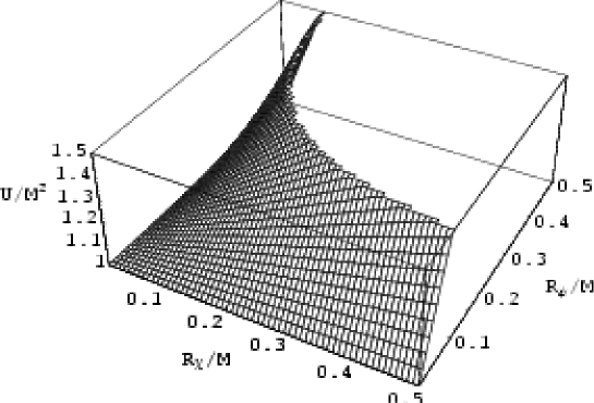
Figure 7.1: The energy per unit length, in unit of $M^{2}$ and at zeroth order, as function of ${\mathcal{X}}$ and $\Psi$ fermion densities plotted in unit of $M$, in the infinite string limit.

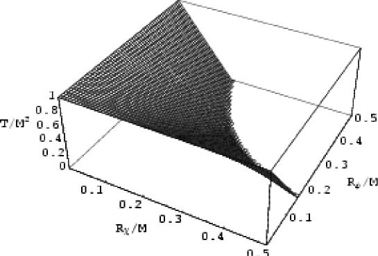
Figure 7.2: The tension, in unit of $M^{2}$ and at zeroth order, as function of ${\mathcal{X}}$ and $\Psi$ fermion densities plotted in unit of $M$, in the infinite string limit.

As expected from their analytical expressions in the infinite string limit, the energy per unit length is always positive and grows with both fermion densities, ${\mathcal{R}}_{\chi}$ and ${\mathcal{R}}_{\psi}$, whereas the tension always decreases and takes negatives values for large fermion densities. Obviously, in the case ${\mathcal{R}}_{\chi}={\mathcal{R}}_{\psi}=0$ there is no current along the string and we recover the Goto-Nambu case, $U=T=M^{2}$. The chiral case, where the fermionic current is lightlike, is obtained for ${\mathcal{R}}_{\chi}=0$, or ${\mathcal{R}}_{\psi}=0$, and also verifies $U=T=M^{2}$ as in the chiral scalar current case [82]. From Eq. (7.125), and in the infinite string limit, the densities for which the tension vanishes verify

$${\mathcal{R}}_{\chi}{\mathcal{R}}_{\psi}=\frac{M^{2}}{4\pi},$$ (7.127)

This curve separates the plane $({\mathcal{R}}_{\chi},{\mathcal{R}}_{\psi})$ in two regions where $T$ is positive near the origin, and negative on the other side (see Fig. 7.3). In the macroscopic formalism of Carter [80, 71, 70, 63], the transverse perturbations propagation speed is given by $c_{{}_{\mathrm{T}}}^{2}=T/U$, and therefore the domains where $T<0$ correspond to strings which are always locally unstable with respect to transverse perturbations.

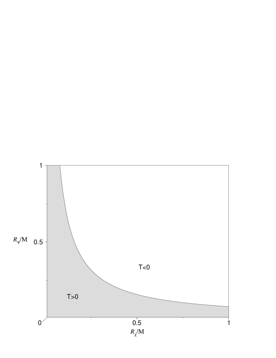
Figure 7.3: Sign of the tension in the $({\mathcal{R}}_{\chi}/M,{\mathcal{R}}_{\psi}/M)$ plane, in the infinite string limit. According to the macroscopic formalism, the string is unstable with respect to transverse perturbations for $T<0$.

The tension of the string becomes negative only for carrier densities close to the mass of the Goto-Nambu string $M$. For such currents, it is necessary to derive the back reaction in order to see how relevant it is for the energy per unit length and tension. Moreover, in a renormalizable model, the vacuum mass acquired by the fermions from their coupling to the Higgs field is less than the Goto-Nambu string mass, and thus, another quantum effects may take place before the negative tension is reached, like tunneling into massive states. Besides, note that $M$, the string unit of mass, arising from non-perturbative effects, may well be much larger than the Higgs boson mass, and so, it is expected that ${\mathcal{R}}_{\chi},{\mathcal{R}}_{\psi}\ll M$. Thus, the no-spring conjecture [278] proposed in the case of bosonic carrier presumably apply to the fermionic carrier case as well. Moreover, the zero mode vacuum effects on energy per unit length and tension appear clearly from Eq. (7.103) as additional string length. The corrected values of the equation of state are therefore obtained by replacing the physical length of the string, $L$, in Eq. (7.124) and Eq. (7.125), by an equivalent length, $L_{{\mathrm{e}}}$ say, which verifies

$$\frac{1}{2L_{\mathrm{e}}^{2}}=\frac{1}{2L^{2}}-\frac{1}{L_{\mathrm{v}}^{2}}.$$ (7.128)

In the particular case where $L_{\mathrm{v}}^{2}=6L^{2}$, it reads $L_{\mathrm{e}}^{2}=(3/2)L^{2}$. On the other hand, the massive vacuum effects certainly shift in a different way $U$ and $T$ by a finite amount as previously discussed, but will not be considered in the following. In the next section, the back reaction is derived in the classical limit in order to find corrected values of energy per unit length and tension. Moreover we shall take care of the finite length of the string $L$, keeping in mind that its value, and consequently the value of $L_{\mathrm{e}}$, have to be larger than $1/M$ since all physical values have been derived in the classical vortex background, i.e., the quantum effects of the Higgs field have been neglected.

7.5.3 Back Reaction

The existence of fermionic currents carrying gauge charge along the string gives rise to new gauge field components, $B_{t}$ and $B_{z}$, from the equations of motion (7.21). These, being coupled with the corresponding currents, provide additional terms in the energy momentum tensor (7.87). As a first step, the new gauge field components are computed numerically from the zero modes solutions of Eq. (7.33). The corrected equation of state is then analytically derived, the numerical dependencies having been isolated in model dependent coefficients.

Back reacted gauge fields

In order to compute the $B_{t}$ and $B_{z}$ fields at first order, we only need the zeroth order values of the zero modes and the vortex background. Let us introduce the dimensionless scaled fields and variables

$$\varphi=\eta H,\quad Q_{\theta}=Q,\quad r=\frac{\varrho}{m_{\mathrm{h}}},$$ (7.129)

with $m_{\mathrm{h}}=\eta\sqrt{\lambda}$ the classical mass of the Higgs field. From the equation of motion (7.16), the orthoradial gauge field $Q$ and $H$ are solution of

$$\frac{{\mathrm{d}}^{2}H}{{\mathrm{d}}\varrho^{2}}+\frac{1}{\varrho}\frac{{\mathrm{d}}H}{{\mathrm{d}}\varrho} = \frac{HQ^{2}}{\varrho^{2}}+\frac{1}{2}H(H^{2}-1),$$ (7.130)

$$\frac{{\mathrm{d}}^{2}Q}{{\mathrm{d}}\varrho^{2}}-\frac{1}{\varrho}\ \frac{{\mathrm{d}}Q}{{\mathrm{d}}\varrho} = \frac{m_{\mathrm{b}}^{2}}{m_{\mathrm{h}}^{2}}H^{2}Q,$$ (7.131)

where $m_{\mathrm{b}}=qc_{\phi}\eta$ is the classical mass of the gauge boson. The numerical solutions of these equations have been computed earlier by many people [23, 282] using relaxation methods [6]. They are presented in Fig. 7.4 for a specific (assumed generic) set of parameters.

Figure 7.4: The solutions of the field equations for the vortex background. The Higgs field, $H$, takes its vacuum expectation value at infinity and the gauge bosons condensate in the vortex.

In the same way, deriving Eq. (7.33) with respect to $\varrho$ yields the right component of the zero mode $Y$ as a solution of

$$\zeta_{1}^{\prime\prime}-\left(\frac{H^{\prime}}{H}+\frac{Q-n}{\varrho}\right)\zeta_{1}^{\prime} + \left[\frac{c_{\chi_{\mathrm{R}}}}{c_{\phi}}\left(\frac{Q-n}{\varrho}\frac{H^{\prime}}{H}+\frac{Q-n}{\varrho^{2}}-\frac{Q^{\prime}}{\varrho}\right)\right.$$ (7.132)

$$- \left.\frac{c_{\chi_{\mathrm{L}}}c_{\chi_{\mathrm{R}}}}{c_{\phi}^{2}}\left(\frac{Q-n}{\varrho}\right)^{2}-\frac{m_{\mathrm{f}}^{2}}{m_{\mathrm{h}}^{2}}H^{2}\right]\zeta_{1}=0,$$

while the left one satisfies

$$i\frac{m_{\mathrm{f}}}{m_{\mathrm{h}}}H\zeta_{4} = \zeta_{1}^{\prime}-\frac{c_{\chi_{\mathrm{R}}}}{c_{\phi}}\frac{Q-n}{\varrho}\zeta_{1},$$ (7.133)

where a prime indicates a derivation with respect to the dimensionless radial variable $\varrho$. The field $\Psi$ verifies similar equations with the transformation, $\zeta\rightarrow\xi$ and $c_{\chi}\rightarrow c_{\psi}$. The numerical integration has been performed with a relaxation method [6] and verified on the original system (7.33) with a shooting method. As a result, the normalized probability densities of the zero modes, $|X|^{2}$ and $|Y|^{2}$, are plotted in Fig. 7.5. The dimensionless radial functions $\tilde{f}_{\chi}$ and $\tilde{f}_{\psi}$ defined from Eq. (7.109) and Eq. (7.110) by

$$\tilde{f}_{\chi}=\frac{2\pi}{m_{\mathrm{h}}^{2}}f_{\chi},\quad\tilde{f}_{\psi}=\frac{2\pi}{m_{\mathrm{h}}^{2}}f_{\psi},$$ (7.134)

are plotted in Fig. 7.6. As expected, the fields are confined in the string core, and so will the corresponding fermionic currents.

Let us define the more relevant components of the backreacted gauge field, $\Delta B=B_{z}-B_{t}$ and $\Sigma B=B_{z}+B_{t}$, with the corresponding dimensionless scaled fields $\Delta\tilde{Q}$ and $\Sigma\tilde{Q}$ defined by

$$\Delta B=\left(\overline{\rho}_{\chi}-\rho_{\chi}\right)\frac{m_{\mathrm{b}}^{2}}{\pi\eta^{2}}\frac{\Delta\tilde{Q}}{qc_{\phi}}, \Sigma B=-\left(\overline{\rho}_{\psi}-\rho_{\psi}\right)\frac{m_{\mathrm{b}}^{2}}{\pi\eta^{2}}\frac{\Sigma\tilde{Q}}{qc_{\phi}}.$$ (7.135)

The equations of motion (7.21) in the classical limit now reads

$$\Delta\tilde{Q}^{\prime\prime}+\frac{1}{\rho}\Delta\tilde{Q}^{\prime}-\frac{m_{\mathrm{b}}^{2}}{m_{\mathrm{h}}^{2}}H^{2}\Delta\tilde{Q}=\frac{\tilde{f}_{\chi}}{qc_{\phi}}, \Sigma\tilde{Q}^{\prime\prime}+\frac{1}{\rho}\Sigma\tilde{Q}^{\prime}-\frac{m_{\mathrm{b}}^{2}}{m_{\mathrm{h}}^{2}}H^{2}\Sigma\tilde{Q}=\frac{\tilde{f}_{\psi}}{qc_{\phi}}.$$ (7.136)

As for fermions, these new gauge fields get their masses from coupling with the Higgs field, and therefore have non-zero mass outside the string core. Moreover, they are generated by fermionic massless currents confined in the core, therefore they also condense in and do not lead to new long-range effects. The solutions of these equations (7.136) have been obtained using, once again, a relaxation method [6] and are represented in Fig. 7.7. Note that owing to the scaled field $\Delta\tilde{Q}$ and $\Sigma\tilde{Q}$, we have separated the numerical dependence in the gauge field and currents from the fermion densities content [see Eq. (7.135)].

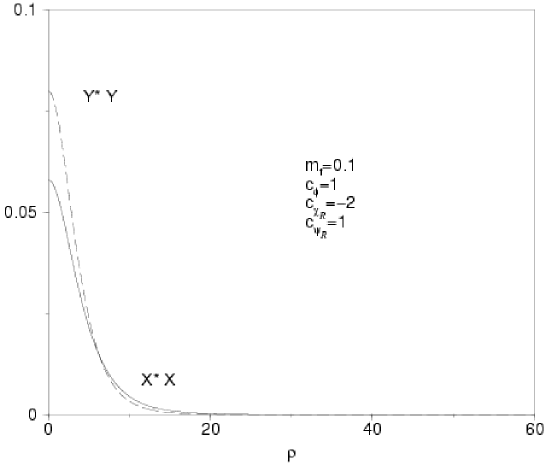
Figure 7.5: The normalized probability densities of the zero modes, $|X|^{2}$ and $|Y|^{2}$. The rapid decay far from the string core reflects the bound state nature of the condensates.

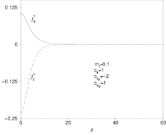
Figure 7.6: The dimensionless radial current functions $\tilde{f}_{\chi}$ and $\tilde{f}_{\psi}$. They can be viewed as the effective transverse density charge carried by the fermion currents. Their sign results in the initial choice of each conserved fermion gauge charge.

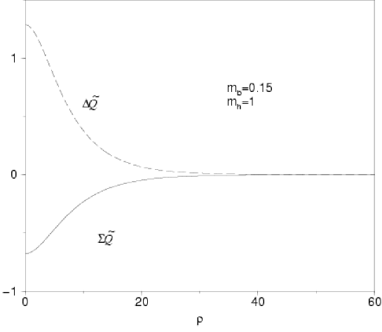
Figure 7.7: The dimensionless backreacted gauge fields $\Delta\tilde{Q}$ and $\Sigma\tilde{Q}$, generated by the fermion currents. They do not lead to new long-range effects since they acquire non-zero mass outside the string core due to their coupling with the Higgs fields.

Up to now, we have computed the fermionic gauge currents along the string as well as the component $B_{t}$ and $B_{z}$, so that the back reaction correction to the energy momentum tensor is computable from Eq. (7.87). As in the previous section, the energy per unit length and tension can be derived in the preferred frame where the stress tensor is diagonal, but now we have to find the eigenvalues of the full two-dimensional energy momentum tensor $\overline{T}^{\alpha\beta}_{{\mathrm{b}}.{\mathrm{r}}.}+\langle\overline{T}^{\alpha\beta}\rangle$, with

$$\overline{T}^{\alpha\beta}_{{\mathrm{b}}.{\mathrm{r}}.}=\int{r\,{\mathrm{d}}r\,{\mathrm{d}}\theta\,T^{\alpha\beta}_{{\mathrm{b}}.{\mathrm{r}}.}}$$ (7.137)

Energy per unit length and tension with back reaction

Using the dimensionless field, $\Delta\tilde{Q}$ and $\Sigma\tilde{Q}$, with the expressions of the currents given in equations (7.107) and (7.108), one gets, after some algebra, the full expression of the stress tensor with corresponding eigenvalues

$$\widehat{U} = M^{2}-I(\Theta_{\chi},\Theta_{\psi}){\widehat{\mathcal{R}}}_{\chi}{\widehat{\mathcal{R}}}_{\psi}+4\pi\sqrt{\left({\widehat{\mathcal{R}}}_{\chi}^{2}-\frac{1}{2L_{\mathrm{e}}^{2}}\right)\left({\widehat{\mathcal{R}}}_{\psi}^{2}-\frac{1}{2L_{\mathrm{e}}^{2}}\right)},$$ (7.138)

$$\widehat{T} = M^{2}-I(\Theta_{\chi},\Theta_{\psi}){\widehat{\mathcal{R}}}_{\chi}{\widehat{\mathcal{R}}}_{\psi}-4\pi\sqrt{\left({\widehat{\mathcal{R}}}_{\chi}^{2}-\frac{1}{2L_{\mathrm{e}}^{2}}\right)\left({\widehat{\mathcal{R}}}_{\psi}^{2}-\frac{1}{2L_{\mathrm{e}}^{2}}\right)},$$ (7.139)

with the scaled state parameters

$${\widehat{\mathcal{R}}}_{\chi} = {\mathcal{R}}_{\chi}\sqrt{1-\frac{m_{\mathrm{b}}^{2}}{2\pi^{2}\eta^{2}}\left(I_{\Delta\chi}-I_{\Delta 2}\right)\sin^{2}{\left(\Theta_{\chi}-\frac{\pi}{4}\right)}},$$ (7.140)

$${\widehat{\mathcal{R}}}_{\psi} = {\mathcal{R}}_{\psi}\sqrt{1-\frac{m_{\mathrm{b}}^{2}}{2\pi^{2}\eta^{2}}\left(I_{\Sigma\psi}-I_{\Sigma 2}\right)\sin^{2}{\left(\Theta_{\psi}-\frac{\pi}{4}\right)}},$$ (7.141)

and the function $I(\Theta_{\chi},\Theta_{\psi})$ defined by

$$I(\Theta_{\chi},\Theta_{\psi}) = \displaystyle\frac{m_{\mathrm{b}}^{2}}{\pi\eta^{2}}\frac{\displaystyle\left(I_{\Sigma\chi}+I_{\Delta\psi}\right)\sin{\left(\Theta_{\chi}-\frac{\pi}{4}\right)}}{\sqrt{\displaystyle 1-\frac{m_{\mathrm{b}}^{2}}{2\pi^{2}\eta^{2}}\left(I_{\Delta\chi}-I_{\Delta 2}\right)\sin^{2}{\left(\Theta_{\chi}-\frac{\pi}{4}\right)}}}$$ (7.142)

$$\times\frac{\sin{\left(\Theta_{\psi}-\frac{\pi}{4}\right)}}{\sqrt{\displaystyle 1-\frac{m_{\mathrm{b}}^{2}}{2\pi^{2}\eta^{2}}\left(I_{\Sigma\psi}-I_{\Sigma 2}\right)\sin^{2}{\left(\Theta_{\psi}-\frac{\pi}{4}\right)}}}$$

The numerical integrations previously carried out appear through pure numbers which depend only on the model parameters. The coupling $B_{\mu}j^{\mu}$ leads to the following quantities

$$I_{\Sigma\chi}=-2\int{\,\varrho\,{\mathrm{d}}\varrho\,\Sigma\tilde{Q}(\varrho)\frac{\tilde{f}_{\chi}(\varrho)}{qc_{\phi}}}, I_{\Delta\psi}=-2\int{\,\varrho\,{\mathrm{d}}\varrho\,\Delta\tilde{Q}(\varrho)\frac{\tilde{f}_{\psi}(\varrho)}{qc_{\phi}}},$$ (7.143)

$$I_{\Sigma\psi}=-2\int{\,\varrho\,{\mathrm{d}}\varrho\,\Sigma\tilde{Q}(\varrho)\frac{\tilde{f}_{\psi}(\varrho)}{qc_{\phi}}}, I_{\Delta\chi}=-2\int{\,\varrho\,{\mathrm{d}}\varrho\,\Delta\tilde{Q}(\varrho)\frac{\tilde{f}_{\chi}(\varrho)}{qc_{\phi}}},$$ (7.144)

while the kinetic contribution of the new gauge fields appears through

$$I_{\Delta 2}=\int{\,\varrho\,{\mathrm{d}}\varrho\,\left[\partial_{\varrho}\Delta\tilde{Q}(\varrho)\right]^{2}}, I_{\Sigma 2}=\int{\,\varrho\,{\mathrm{d}}\varrho\,\left[\partial_{\varrho}\Sigma\tilde{Q}(\varrho)\right]^{2}}.$$ (7.145)

By means of the equations of motion (7.136) and the constant sign of $\Delta\tilde{Q}$ and $\Sigma\tilde{Q}$, $I_{\Delta\chi}$ and $I_{\Sigma\psi}$ are found to be always positive. Intuitively, as in electromagnetism, the gauge field generated from charge currents tends to resist to the currents which give birth to it. In our case, the back reaction actually damps the weight of the charge carriers in the energy per unit length and tension. In fact, the relevant state parameters are now ${\widehat{\mathcal{R}}}$ instead of ${\mathcal{R}}$ with ${\widehat{\mathcal{R}}}<{\mathcal{R}}$ since $I_{\Delta\chi}$ and $I_{\Sigma\psi}$ are positive. Moreover, numerical calculations show that the kinetic contribution numbers (7.145) are always one order of magnitude smaller than those resulting in the coupling between gauge fields and currents (7.143), as expected for reasonable backreacted gauge field since they only involve the square gradient of these fields [see Eq. (7.145)]. However, there is an additional term involving new dependence in the asymmetry between particles and anti-particles through the $I(\Theta_{\chi},\Theta_{\psi})$ function. In order to understand this point physically, let us derive the magnitude of the gauge current carried by the fermions. From Eq. (7.107) and Eq. (7.108), once the transverse coordinates have been integrated over, the dimensionless magnitude reads

$$\tilde{\overline{j}}^{2}=\frac{\displaystyle 2(2qc_{\phi})^{2}\tilde{F}_{\chi}\tilde{F_{\psi}}\sin{\left(\Theta_{\chi}-\frac{\pi}{4}\right)}\sin{\left(\Theta_{\psi}-\frac{\pi}{4}\right)}{\widehat{\mathcal{R}}}_{\chi}{\widehat{\mathcal{R}}}_{\psi}}{\sqrt{\displaystyle 1-\frac{m_{\mathrm{b}}^{2}}{2\pi^{2}\eta^{2}}\left(I_{\Delta\chi}-I_{\Delta 2}\right)\sin^{2}{\left(\Theta_{\chi}-\frac{\pi}{4}\right)}}\sqrt{\displaystyle 1-\frac{m_{\mathrm{b}}^{2}}{2\pi^{2}\eta^{2}}\left(I_{\Sigma\psi}-I_{\Sigma 2}\right)\sin^{2}{\left(\Theta_{\psi}-\frac{\pi}{4}\right)}}},$$ (7.146)

with the dimensionless constants are

$$\tilde{F}_{\chi}=\int{\,\varrho\,{\mathrm{d}}\varrho\,\frac{\tilde{f}_{\chi}(\varrho)}{qc_{\phi}}}, \tilde{F}_{\psi}=\int{\,\varrho\,{\mathrm{d}}\varrho\,\frac{\tilde{f}_{\psi}(\varrho)}{qc_{\phi}}}.$$ (7.147)

These numbers can be viewed as the effective charge carried by the fermionic gauge currents since

$$\frac{\tilde{\overline{j}}^{2}}{(2qc_{\phi})^{2}\tilde{F_{\chi}}\tilde{F_{\psi}}}=\frac{\overline{{\mathcal{C}}}^{2}}{4}.$$ (7.148)

The function $I(\Theta_{\chi},\Theta_{\psi})$ therefore verifies

$$I(\Theta_{\chi},\Theta_{\psi}){\widehat{\mathcal{R}}}_{\chi}{\widehat{\mathcal{R}}}_{\psi}=\frac{I_{\Sigma\chi}+I_{\Delta\psi}}{8\pi\tilde{F}_{\chi}\tilde{F}_{\psi}}\,\tilde{\overline{j}}^{2},$$ (7.149)

and, as before, according to Eq. (7.136), $(I_{\Sigma\chi}+I_{\Delta\psi})/(\tilde{F}_{\chi}\tilde{F}_{\psi})$ is always positive, so the sign of $I$ directly reflects the spacelike or timelike nature of the current. Thus, in addition to the back reaction damping effect, there is a correction to the energy per unit length and tension directly proportional to the magnitude of the fermionic current. Note that this effect appears as a correction due to back reaction and not, as it is the case for cosmic string with bosonic current carriers, at the zeroth order [282].

Equation of state with back reaction

Unfortunately, the corrected expressions of the line density energy and tension involve four independent state parameters, and consequently are not easily representable. However, they can be studied as functions of the damped fermion densities ${\widehat{\mathcal{R}}}$, modified only by the function $I(\Theta_{\chi},\Theta_{\psi})$ which quantifies the efficiency of the fermionic currents in generating backreacted gauge fields. In this way, the comparison with the zeroth order case is all the more so easy.

The study of the surfaces defined by $\widehat{U}$ and $\widehat{T}$ in the plane $({\widehat{\mathcal{R}}}_{\chi},{\widehat{\mathcal{R}}}_{\psi})$ is less canonical than at zeroth order. Three critical values of the function $I$ are found to modify the behaviors of the tension and energy per unit length, namely, $-4\pi$, $0$, and $4\pi$. However, only small values of $I$ are reasonable in this model as it is discussed in the next section. This analysis is consequently constraints to values of $|I|<4\pi$.

Energy per unit length.

The line density energy follows different behaviors according to the value of $I$.

The first and simplest case $I<0$, obtained for spacelike fermionic gauge currents, is very similar to the zeroth order case, and the energy per unit length just grows a bit faster with the damped fermion densities ${\widehat{\mathcal{R}}}_{\chi}$ and ${\widehat{\mathcal{R}}}_{\psi}$, as on Fig. 7.8.

For timelike currents, $I>0$, we find that the back reaction damps the growth of the density line energy with the fermion densities. As a result the line density energy seems to decrease in some regions, and the stationary curves of $\widehat{U}$ with respect to ${\widehat{\mathcal{R}}}_{\chi}$ are given, from Eq. (7.138), by

$$\frac{\partial{\widehat{U}}}{\partial{\widehat{\mathcal{R}}}_{\chi}}=0 \Leftrightarrow {\widehat{\mathcal{R}}}_{\psi}=\frac{2\pi}{L_{\mathrm{e}}}{\widehat{\mathcal{R}}}_{\chi}\sqrt{\displaystyle\frac{2}{\displaystyle\frac{I^{2}}{2L_{\mathrm{e}}^{2}}+(16\pi^{2}-I^{2}){\widehat{\mathcal{R}}}_{\chi}^{2}}},$$ (7.150)

and thanks to the symmetry between ${\widehat{\mathcal{R}}}_{\chi}$ and ${\widehat{\mathcal{R}}}_{\psi}$, similar equations are obtained for $\partial\widehat{U}/\partial{\widehat{\mathcal{R}}}_{\psi}=0$. Finally, the variation domains of the line density energy are represented in Fig. 7.9 for $0<I<4\pi$. The first discrete values of the fermion densities (the length of the string is finite) have been represented by dots in the $({\widehat{\mathcal{R}}}_{\chi}$,${\widehat{\mathcal{R}}}_{\psi})$-plane, and as can be seen in Fig. 7.9, for reasonable values of $I$, there is no available quantum state inside the tiny decreasing regions. Consequently, the density line energy always grows with the fermions densities and remains positive. Since the stationary curves of $\widehat{U}$ are asymptotically proportional to $1/L_{\mathrm{e}}<1/L$ [see Eq. (7.150)], they coincide with the axis in the infinite string limit. The surface describing $\widehat{U}({\widehat{\mathcal{R}}}_{\chi},{\widehat{\mathcal{R}}}_{\psi})$ has also been plotted in Fig. 7.9 in unit normalized to $M^{2}$, and for minimal acceptable value of $L_{\mathrm{e}}=10/M$ just in order to show the influence of the finite length.

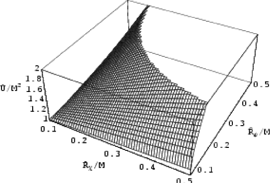
Figure 7.8: The energy per unit length in unit of $M^{2}$ as function of ${\widehat{\mathcal{R}}}_{\chi}/M$ and ${\widehat{\mathcal{R}}}_{\psi}/M$, for spacelike currents with $I(\Theta_{\chi},\Theta_{\psi})<0$. The influence of the finite length of the string just appears near the axes.

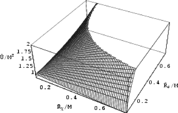
Figure 7.9: Variation domains of the energy per unit length, plotted in unit of $M^{2}$, in the $({\widehat{\mathcal{R}}}_{\chi}/M,{\widehat{\mathcal{R}}}_{\psi}/M)$ plane for timelike currents with $0<I<4\pi$. The vertical hatched regions define domains where the line density energy could decrease with ${\widehat{\mathcal{R}}}_{\chi}$ whereas the horizontal ones are regions where the line density energy could decrease with ${\widehat{\mathcal{R}}}_{\psi}$. On one hand, these domains are asymptotically limited by the curves ${\widehat{\mathcal{R}}}=(2\pi/L_{\mathrm{e}})\sqrt{2/(16\pi^{2}-I^{2})}$ and therefore coincide with the axis for large values of $L_{\mathrm{e}}$. On the other hand, for reasonable values of $I\ll 4\pi$, there is no accessible quantum state inside, the first one being shown as a dot. As a result the energy per unit length always grows with the parameters ${\widehat{\mathcal{R}}}$ and is always positive.

Tension.

The study of the tension with respect to the fermion densities is performed in the same way. As before the stationary curves of $\widehat{T}$ with respect to ${\widehat{\mathcal{R}}}_{\chi}$ or ${\widehat{\mathcal{R}}}_{\psi}$ are found from Eq. (7.139), and follow the same equation as those of the energy per unit length in Eq. (7.150), although the variation domains are not the same and have been plotted in Fig. 7.11 for different values of the function $I$.

For timelike fermionic gauge current, $I>0$, the tension decreases faster than in the zeroth order case, with the damped fermionic densities ${\widehat{\mathcal{R}}}_{\chi}$ and ${\widehat{\mathcal{R}}}_{\psi}$ as on Fig. 7.10, and reaches negative values at large densities (see Fig. 7.12). The back reaction just increases the slope of the surface, and thus, the negative values are reached more rapidly. As for the energy per unit length, the equivalent length was chosen equal to $L_{\mathrm{e}}=10/M$ in the following figures.

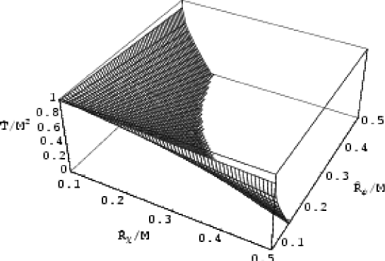
Figure 7.10: The tension for timelike currents with $I>0$, plotted in unit of $M^{2}$ in the $({\widehat{\mathcal{R}}}_{\chi}/M,{\widehat{\mathcal{R}}}_{\psi}/M)$ plane. Note the shift near the axes due to the finite length of the string.

For spacelike fermionic gauge currents, $-4\pi<I<0$, the back reaction damps the decrease of the tension with respect to the damped fermion densities. There are also tiny regions near the axis, with areas inversely proportional to $L_{\mathrm{e}}$, and where $\widehat{T}$ could grow with respect to one of the state parameters ${\widehat{\mathcal{R}}}_{\chi}$ or ${\widehat{\mathcal{R}}}_{\psi}$ (see Fig. 7.11). As previously, for reasonable values of $I$, the first discrete values of the parameters are out of these domains, and the tension always decreases with both fermion densities. Finally, the tension reaches negative values at large damped fermion densities (see Fig. 7.12).

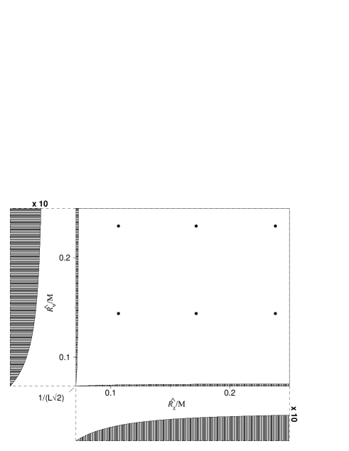
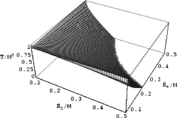
Figure 7.11: Variation domains of the tension, plotted in unit of $M^{2}$, for spacelike currents with $-4\pi<I<0$, in the $({\widehat{\mathcal{R}}}_{\chi}/M,{\widehat{\mathcal{R}}}_{\psi}/M)$ plane. These regions have the same geometrical properties as the line density energy ones in Fig. 7.9, but this time, the zones with vertical hatches are domains where $\widehat{T}$ could grow with respect to ${\widehat{\mathcal{R}}}_{\chi}$, whereas the horizontal ones correspond to growth with respect to ${\widehat{\mathcal{R}}}_{\psi}$. For reasonable values of $I$, the discrete values of ${\widehat{\mathcal{R}}}$, represented by dots, are out of these regions, and the tension always decrease with both fermion densities.

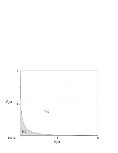
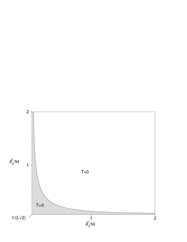
Figure 7.12: Sign of the tension for timelike currents with $I>0$, and spacelike currents with $-4\pi<I<0$, the curves have been plotted with $L_{\mathrm{e}}=10/M$ in aim at clearly separating the various regions. In the timelike case, the domain where the tension is positive is closed, the null tension curves intersecting the axes at ${\widehat{\mathcal{R}}}=\sqrt{2}L_{\mathrm{e}}M^{2}/I$, whereas for spacelike currents, the null tension curves tends asymptotically to ${\widehat{\mathcal{R}}}=(2\pi/L_{\mathrm{e}})\sqrt{2/(16\pi^{2}-I^{2})}$. Recall that the regions where $T<0$ are unstable with respect to transverse string perturbations according to the macroscopic formalism.

Relevant values of the parameters

The previous derivation of the back reaction is built on the classical vortex background and it is acceptable only if the backreacted gauge fields do not perturb appreciably the Higgs and orthoradial gauge fields profiles (see Fig. 7.4). From Eq. (7.16), it will be the case only if $Q^{t}Q_{t}$ and $Q^{z}Q_{z}$ can be neglected compared to $Q^{\theta}Q_{\theta}$. From Eq. (7.135), and $Q_{\theta}Q^{\theta}\sim m_{\mathrm{b}}^{2}$, this condition reads

$$\frac{(qc_{\phi})^{2}\Delta B\Sigma B}{Q_{\theta}Q^{\theta}}\sim\frac{{\mathcal{R}}_{\chi}{\mathcal{R}}_{\psi}\sin{\left(\Theta_{\chi}-\frac{\pi}{4}\right)}\sin{\left(\Theta_{\psi}-\frac{\pi}{4}\right)}}{\pi\eta^{2}}\frac{m_{\mathrm{b}}^{2}}{\pi\eta^{2}}\Delta\tilde{Q}\Sigma\tilde{Q} \ll 1,$$ (7.151)

or as function of $I(\Theta_{\psi},\Theta_{\chi})$ and the damped fermion densities,

$$I(\Theta_{\chi},\Theta_{\psi})\frac{{\widehat{\mathcal{R}}}_{\chi}{\widehat{\mathcal{R}}}_{\psi}}{\pi\eta^{2}} \ll 1.$$ (7.152)

This condition is satisfied for damped fermion densities small compared to the string energy scale, or for tiny values of the function $I(\Theta_{\psi},\Theta_{\chi})$. Moreover, the backreacted gauge fields need to be small in order to not significantly perturb the zero modes. From the equations of motion (7.22) and (7.24), this condition leads to $\Delta B,\Sigma B\ll{\mathcal{R}}$ and from Eq. (7.135) to

$$\frac{m_{\mathrm{b}}^{2}}{\eta^{2}}\frac{c_{\psi(\chi)}}{c_{\phi}}\Sigma(\Delta)\tilde{Q}(0)\ll 1.$$ (7.153)

On the other hand, the maximum value of $I$ in Eq. (7.142) is clearly obtained when there are only particles or anti-particles trapped in the string ($\Theta=0$ or $\Theta=\pi$), and deriving the order of magnitude of the numerical integral in Eq. (7.143), using equations (7.136) and (7.109)-(7.110), one shows that the large values of $I$ (as $I>4\pi$) can only be obtained for model parameters which verify

$$\frac{m_{\mathrm{b}}^{2}}{\eta^{2}}\frac{c_{\psi(\chi)}}{c_{\phi}}\Sigma(\Delta)\tilde{Q}(0)>1.$$ (7.154)

As a result, in order for the backreacted gauge fields not to modify the equations of motion of the fermions at first order, the function $I$ has to be much smaller than $4\pi$. If it is not the case, then the previous zero modes are no longer valid solutions and the relevant equations of motion, in the case of the $\Psi$ fermions, now read, from Eq. (7.22)

$$\begin{array}[]{lll}\vspace{4pt}\displaystyle\left[\frac{{\mathrm{d}}\xi_{1}}{{\mathrm{d}}r}+\frac{1}{r}\left(-qc_{\psi_{\mathrm{R}}}B+m_{1}\right)\xi_{1}\right]-ig\varphi\xi_{4}&=&i[\mp(k+\omega)+qc_{\psi_{\mathrm{R}}}\Delta B]\xi_{2},\\ \vspace{4pt}\displaystyle\left[\frac{{\mathrm{d}}\xi_{2}}{{\mathrm{d}}r}+\frac{1}{r}\left(qc_{\psi_{\mathrm{R}}}B-m_{2}\right)\xi_{2}\right]-ig\varphi\xi_{3}&=&i[\pm(k-\omega)-qc_{\psi_{\mathrm{R}}}\Sigma B]\xi_{1},\\ \vspace{4pt}\displaystyle\left[\frac{{\mathrm{d}}\xi_{3}}{{\mathrm{d}}r}+\frac{1}{r}\left(-qc_{\psi_{\mathrm{L}}}B+m_{3}\right)\xi_{3}\right]+ig\varphi\xi_{2}&=&i[\mp(k-\omega)+qc_{\psi_{\mathrm{L}}}\Sigma B]\xi_{4},\\ \displaystyle\left[\frac{{\mathrm{d}}\xi_{4}}{{\mathrm{d}}r}+\frac{1}{r}\left(qc_{\psi_{\mathrm{L}}}B-m_{4}\right)\xi_{4}\right]+ig\varphi\xi_{1}&=&i[\pm(k+\omega)-qc_{\psi_{\mathrm{L}}}\Delta B]\xi_{3},\end{array}$$ (7.155)

where the angular dependence has not been written owing to Eq. (7.31) and assuming $m_{1}=m_{3}+n$. The zero modes seem to acquire an effective mass proportional to $\Delta B$ or $\Sigma B$. More precisely, they are no longer eigenstates of the $\gamma^{0}\gamma^{3}$ operator since new spinor components appear [$\xi_{1}$, $\xi_{4}$ here, see Eq. (7.33) and Eq. (7.34)]. It is clearly a second order effect since the gauge coupling constant $q$ can be removed in the previous equations (7.155) using Eq. (7.135) and assuming

$$\xi=X+q^{2}\delta\xi,$$ (7.156)

with $X$ the zero mode solution $k=-\omega$ for $\Psi$ fermions [see Eq. (7.43)], and $q^{2}\delta\xi$ the perturbation induced by the back reaction [302]. As a result, for strong back reaction, the semi-classical approach can no longer be used, since such second order effects appear as the semi-classical manifestations of the one loop quantum corrections, and thus, only a full quantum theory would be well defined. However, if there is only one kind of fermion trapped in the string, $\Psi$ say, the zero modes are not affected by the back reaction since $\Delta B$ is only generated from the ${\mathcal{X}}$ current, and therefore vanishes [see Eq. (7.136)], so $\xi=X$ is always solution of the equations of motion (7.155), and identically for the ${\mathcal{X}}$ zero modes alone [256]. Note, that there is no contradiction with the usual index theorem since it is derived for Dirac operators, and thus without backreacted fields. This just shows that the modes propagating in the vortex with strong backreacted gauge fields are no longer well described by the usual zero modes. Physically, it might be the signature of a tunneling of the zero modes to another states. The massive modes which have not been considered here could be more relevant in such cases.

On the other hand, the shape of the string might allow the fermion densities ${\widehat{\mathcal{R}}}_{\chi}$ and ${\widehat{\mathcal{R}}}_{\psi}$ to reach the tiny regions where the energy decreases with one of them (see Fig. 7.9), by means of the zero mode vacuum quantum effects. The present toy model does not involve the effect of the radius of curvature $R$ of the string, and it is reasonable that the contribution of the zero mode vacuum to the energy per unit length involves $R$ through a redefinition of $L_{\mathrm{e}}$. If $L_{\mathrm{e}}$ becomes smaller than $L$, the first discrete values of the fermion densities could be inside the hatched regions in Fig. 7.9, since the discrete values of the fermion densities only depend on the physical length of the string $L$. Note that it would therefore be necessary that the zero mode vacuum energy is negative, which is not the case without curvature in the simple framework of Sec. 7.4.2. Such effects could be relevant for vorton stability, as, for a small radius of curvature, the string could become unstable to fermion condensation.

Finally, the model can be used only at the tree order, and the conditions (7.152) and (7.153) are the validity criteria of the above derivations.

7.6 Comparison with the scalar case

Owing to the fermionic two-dimensional quantization along the string, the energy per unit length and the tension of a string carrying massless fermionic currents have been derived up to the first order in back reaction corrections. The state of the string is found to be well defined with four state parameters which are the densities of each fermion trapped in the string, and asymmetry angles between particles and anti-particles in each fermion family. It seems quite different than the bosonic charge carriers case, where the current magnitude is the only relevant state parameter [282], however, this is the result of the allowed purely classical approach where the superposition of many quantum states can be view as only one classical state owing to the bosonic nature of the charge carriers. As a result, there is a degeneracy between the number of bosons trapped in the string and the charge current. The quantization introduced to deal with fermions naturally leads to separate the charge current from the particle current through the existence of anti-particle exitations. Moreover, the magnitude of the current can only modify the equation of state at non-zeroth order because the chiral nature of fermions trapped in the string requires simultaneous exitations between the two families to lead to non-lightlike charge currents.

Nevertheless, some global comparisons can be made with the scalar case. First, for reasonable values of $I\ll 4\pi$, the energy per unit length grows with the fermionic densities, whereas the tension decreases with them. However, note the relevant parameter for the change in behaviors of the tension and line density energy is the function $I(\Theta_{\chi},\Theta_{\psi})$ instead of the current magnitude in the scalar case. As it was said, $I$ quantifies, through the asymmetry between the number of particles and anti-particles trapped in the string, the efficiency of the charge current per particle to be timelike or spacelike. The more positive is $I$, the more timelike the fermionic charge current per particle will be, and conversely the more negative $I$ is, the more spacelike it will be. Once again, this difference with the scalar case appears as a result of the degeneracy breaking between particle current and charge current due to the fermionic nature of the charge carriers.

The stability of the string with respect to transverse perturbations is given from the macroscopic formalism by the sign of the tension (for line density energy positive) [80, 71, 70, 63], and we find that instabilities always occur for densities roughly close to $M/\sqrt{4\pi+I}$, in finite domain for timelike current, in infinite one for spacelike currents with $-4\pi<I<0$. Another new results are obtained from the multi-dimensional properties of the equation of state, in particular the problem of stability with respect to longitudinal perturbations differs from the scalar barotropic case where the longitudinal perturbations propagation speed is given by $c_{{}_{\mathrm{L}}}^{2}=-dT/dU$ [80, 71, 70, 63], and therefore its two-dimensional form has to be derived to conclude on these kinds of instabilities. Nevertheless, by analogy with the scalar case, since, in the non-perturbed case and in the infinite string limit, the equation of state verifies $U+T=2M^{2}$ [283], the longitudinal perturbation propagation speed might be close to the speed of the light, even with small back reaction, and therefore, only transverse stability would be relevant in macroscopic string stability with massless fermionic currents.

7.7 Conclusion

The energy per unit length and the tension of a cosmic string carrying fermionic massless currents were derived in the frame of the Witten model in the neutral limit. Contrary to bosonic charge carriers, the two-dimensional quantization required to deal with fermions, leads to more than one state parameter in order to yield a well-defined equation of state. They can be chosen, at zeroth order, as fermion densities trapped in the string regardless of charge conjugation. The minimal back reaction correction appears through the fermionic charge current magnitude which involves the asymmetry angles between the number of particles and anti-particles trapped in the string, and which might be identified with the baryonic number of the plasma in which the string was formed during the phase transition. As a result, it is shown that fermionic charge currents can be lightlike, spacelike as well as timelike. Moreover the line energy density and the tension evolve globally as in the bosonic charge carriers case, but it was found that the tension can take negative values in extreme regions where the fermion densities are close to the string mass, and where the string is therefore unstable with respect to transverse perturbations according to the macroscopic formalism.

The present model has been built on the generic existence of fermionic zero modes in the string and follows only a semi-classical approach. It is no longer valid for higher corrections in the back reaction when they modify notably the vortex background and seem to give effective mass to the previous zero modes. It may be conjectured, at this stage, that in a full quantum theory, the quantum loop corrections give mass to the zero modes for high currents and consequently might lead to their decay by the mean of massive states. Only chiral charge currents could be stable on cosmic string carrying large fermionic massless currents in such a case. Another possible effect, relevant for vortons stability, may be expected for loops with small radius of curvature, by means of the vacuum effects which could render the loop unstable to fermion condensation.

It will be interesting to quantify such modifications on the equation of state in future works, as the effects of worldsheet curvature, and the modification of the density line energy and tension by the massive bound states. The field of validity of the model could therefore be extended to higher energy scales which would be more relevant for vortons and string formation.

Acknowledgments

I would like to thank P. Peter for many fruitful discussions, and for his help to clarify the presentation. I also wish to thank B. Carter who helped me to enlighten some aspect of the subject.

Chapitre 8 Approche macroscopique (article)

Dans le chapitre précédent, la quantification des modes zéros le long de la corde a permis de montrer que, lorsque la rétroaction était négligée, la dynamique de la corde était régie par une équation d’état de type trace fixée $U+T=2M^{2}$. Bien que la quantification introduise naturellement plus d’un paramètre d’état, il doit être possible, par le formalisme covariant, de redéfinir un paramètre effectif à partir de cette équation d’état.

Après avoir justifié l’approximation de température nulle utilisée dans la quantification (voir Chap. 7), la relation $U+T=2M^{2}$ est retrouvée par une approche purement macroscopique. La description lagrangienne permet ensuite d’en définir une fonction maîtresse de dépendant que d’un seul paramètre d’état. Ce chapitre est essentiellement un complément aux proceedings de la conférence des  [283].

Fermionic current-carrying cosmic strings:
zero-temperature limit and equation of state

Patrick Peter and Christophe Ringeval

Institut d’Astrophysique de Paris, 98bis boulevard Arago, 75014 Paris, France.

The equation of state for a superconducting cosmic string whose current is due to fermionic zero modes is derived analytically in the case where the back reaction of the fermions to the background is neglected. It is first shown that the zero mode fermions follow a zero temperature distribution because of their interactions (or lack thereof) with the string-forming Higgs and gauge fields. It is then found that the energy per unit length $U$ and the tension $T$ are related to the background string mass $m$ through the simple relation $U+T=2m^{2}$. Cosmological consequences are briefly discussed.

8.1 Introduction

Topological defects [109] have been considered in various physical situations, e.g. in the context of condensed matter and cosmology [211, 210, 341, 178]. In many cases of interest in cosmology [31, 47, 13, 48], they can be approximated as structureless, the relevant dynamics being often assumed not to depend on any specific choice of their internal content. For cosmic defects, this internal content would correspond to the particles that couple to the string-forming Higgs field [362]. However, in the latter example of cosmic strings, it was shown that such a structure might lead to drastic modifications not only of these object dynamics [80, 71, 70, 63, 282], which could be seen as a mere academic situation given our present ignorance on their very existence, but also, because of the appearance of new accessible equilibrium states, of the cosmological setting, leading in some instances to actual catastrophes [103, 67, 54, 297]. To make a long story short, let us just say that currents imply a breakdown of the Lorentz-boost invariance along the string worldsheet, thereby allowing loop configurations to rotate, the centrifugal force hereby induced having the ability to sustain the loop tendency to shrink because of the tension. The resulting states, called vortons, might be stable even over cosmological timescales, scaling as matter and thus rapidly coming to dominate the Universe evolution, in contradiction with the observations. This leads to constraints on the particle physics theories that predict them at energy scales that are believed to be unreachable experimentally (in accelerators say) in the foreseeable future.

Unfortunately, it appears that the string structure, contrary to their counterparts as fundamental objects [285], is not determined by any consistency relation, and is therefore somehow arbitrary, at least at the effective description level [362]. This means in practice that in order to be able to tell anything relevant to (cosmic) string cosmology, one needs to set up a complete underlying microscopic model, arising say, from ones favorite Grand Unified Theory (GUT) [108] or some low-energy approximation of some superstring-inspired model [112, 20, 83, 171, 36].

Some generic constructions can however be arranged, as was shown to be the case whence a bosonic condensate gets frozen in the string core [80, 71, 70, 63, 282]. In such a situation, the boson field phase $\varphi$, thanks to a random Kibble-like mechanism, may wind along the string itself, thereby producing a current that turns out to be essentially a function of a single state parameter $w$, thus expressible as a phase gradient as

$$w\equiv\kappa_{0}\gamma^{ab}\partial_{a}\varphi\partial_{b}\varphi,$$ (8.1)

with indices $a,b,...$ varying within the string worldsheet coordinates defined by the relations

$$x^{\mu}=X^{\mu}_{{}_{{\mathrm{S}}}}(\xi^{a}),\ \ \ \ \ \ \xi^{a}\in\{\tau,\sigma\},$$ (8.2)

and $\gamma^{ab}$ the inverse of the induced metric defined with the background metric $g_{\mu\nu}$ as

$$\gamma_{ab}=g_{\mu\nu}{\partial X^{\mu}_{{}_{{\mathrm{S}}}}\over\partial\xi^{a}}{\partial X^{\nu}_{{}_{{\mathrm{S}}}}\over\partial\xi^{b}}.$$ (8.3)

A straightforward generalization of the Nambu-Goto action is then provided by the $w-$weighted measure as

$${\cal S}=-m^{2}\int\hbox{d}^{2}\xi\sqrt{-\gamma}{\cal L}\{w\},$$ (8.4)

with $m$ the typical mass scale of symmetry breaking leading to string formation and $\gamma$ the determinant of the induced metric (8.3). Reasonable microscopic models [76] then yield approximate forms for the Lagrangian function ${\cal L}\{w\}$, out of which the dynamical properties of the corresponding strings can be derived [224, 63, 144].

Such a description remains however essentially classical even though an alternative formalism, also proposed by Carter [62], in terms of a dilatonic model, appears more suitable for quantization. This last formalism however, being fully two-dimensional, cannot be used to derive interesting quantities such as the relevant cross-sections for trapped excitations to leave the string worldsheet. This is unfortunate since this is precisely the information one would need for cosmological applications [103, 67, 54, 108].

It would therefore seem that by considering fermionic current carriers instead of bosonic ones, one would, because of the intrinsically quantum nature of fermions, obtain a more appropriate description [108, 303]. Besides, fermions are trapped in topological defects because of Yukawa couplings with the string forming Higgs field in the form of zero modes [195], so that their dynamics is described by simple (although coupled) Dirac equations, which are linear. In the bosonic case, the non-linear (quartic) term is essential in order to ensure the dynamical stability of the condensate so that a solitonic treatment [87, 327, 290, 193] seems the only way to deal with the underlying quantum physics. This fact dramatically complicates matters and as a result, a complete description yet fails to exist.

However, the fermionic case is not that simple either as here, one faces another technical difficulty for the classical description: it can be shown that there doesn’t exist a simple state parameter [303]. An arbitrary spacelike or timelike current can only be built out of at least two opposite chirality spinor fields and will be given by the knowledge of four occupation numbers per unit length. As this is true in particular at least in the zero-temperature limit, we shall be concerned here first with this limit whose validity was assumed to depend on the particular model under consideration [108]. In the following section, we show that setting the temperature to zero is always a good approximation because of the couplings between the fermionic fields and the string-forming Higgs and gauge fields. These results would seem to imply that the previously derived macroscopic formalism is irrelevant to the fermionic situation (see Ref. [70] for a many-parameter formalism). In practice however, as a simple relationship between the energy per unit length and the tension can be found for fermionic currents, the single state parameter formalism can be used that permits to draw some cosmological consequences.

8.2 The zero-temperature limit

In order to have an arbitrary current built upon fermionic fields, one needs at least two Dirac fermions [362] $\Psi$ and $\chi$ say, coupled to the string-forming Higgs field $\Phi$ through Yukawa terms as well as to the associated gauge field $B_{\mu}$, the later acquiring a mass from the vacuum expectation value (VEV) of the Higgs field. Fermions may condense in the string core in the form of zero modes, and by filling up the accessible states, one forms a current which can be timelike, spacelike, or lightlike. If one wants to give a classical description of such a current-carrying string, one must be in a configuration for which quantum effects are negligible. Such quantum effects, as for instance tunneling outside the vortex, will indeed be negligible provided most of the fermions are on energy levels whose excitation energy is much below their vacuum mass, the latter thus playing the role of a Fermi energy.

As a result, if a temperature may be defined for the fermions along the vortex, quantum effects will be negligible if the temperature is small compared to the vacuum mass of the fermions, which essentially imply a zero temperature state. Note that the situation we are having in mind is reached only whenever the background temperature is low compared to that at which the string formed for otherwise interactions with the surrounding plasma could populate the high energy levels. In practice, this is what will happen at the time of string formation, and if the fermions did not interact at all, or only through time reversible interactions, one would be left with a frozen distribution corresponding to a high temperature state [78].

That this is not the case can be seen through an exhaustive list of all the possible fermion interactions. For that purpose, it must be emphasized that fermionic condensates arise in the string core in the form of zero modes, i.e. chiral states. One has essentially two coupling possibilities, namely a coupling of the fermion with the Higgs field or with the gauge field, illustrated on the figure. The first case (diagram $a$) is seen to vanish identically in the case of a chiral mode [303] so we shall not consider it. The second case is more interesting and comes from the second diagram ($b$) of the figure. In this case, any trapped fermionic zero mode is seen to be able to radiate a gauge vector boson. These terms do not vanish identically, and in fact can be seen to be the source for some back reacted components of the gauge field: as all the vectors emitted this way will eventually condense into a classical field, this diagram contributes to a small (and indeed usually negligible [303]) contribution in the energy per unit length and tension.

Figure 8.1: Exhaustive list of all the possible interaction terms between fermions and Higgs and gauge fields. $(a)$ Higgs radiation by a fermion field denoted by $\psi$ or $\chi$ (two fermion at least are necessary in order to generate an arbitrary kind of current), $(b)$ gauge boson radiation, $(c)$ coupling between the various fermion fields.

Finally the third term, $(c)$, of the figure, represents a would-be interaction term between the fermions that could be responsible for an equilibrium configuration. When one considers only zero modes in a usual model, such a term actually vanishes because both fermions must have opposite chiralities in order for the theory to be well defined. As a result, interactions between fermions turn out to be negligible.

We are now in a position to understand the microphysics of what might happen inside a fermionic current-carrying cosmic string. First, when the fermions become trapped in the string core, they do so on arbitrary high energy levels inside the string. Then, they have the possibility to radiate most of their energy away in the form of the vector field, thereby creating the back reacted component. Note that the vector field itself can also interact with the Higgs field thereby producing an effective lack of symmetry between diagram $(b)$ and its time reversed counterpart. This implies that the overall effect is indeed a radiative decay and not an equilibrium. Thus, all the populated states end up being the lowest reachable states. In practice, that means that the effective temperature of the fermion gas is vanishing. Moreover, such a configuration in turn is stable as no interaction between the various fermion field can be present.

8.3 Fermionic string equation of state

As was discussed above, fermions that are coupled to the Higgs field may be bound to cosmic strings in the form of zero modes [362, 303, 195] and therefore the current they generate arises from lightlike components. We recall briefly the formalism necessary to handle this case and then move on to derive the resulting stress-energy tensor as well as a simple relationship relating its eigenvalues. This leads to a plausible classical description in terms of a state parameter whose validity is discussed.

8.3.1 Stress-energy tensor and equation of state

Chiral currents have special properties and need be studied on their own. As was shown earlier, a phase gradient formalism hold for them, similar to the $\sigma-$model [62] with vanishing potential, namely [82]

$${\cal S}_{\sigma}=-\int\hbox{d}^{2}\xi\sqrt{-\gamma}\left(m^{2}+{1\over 2}\psi^{2}\gamma^{ab}\partial_{a}\varphi\partial_{b}\varphi\right),$$ (8.5)

where the normalization constant $\kappa_{0}$ of Eq. (8.1) in the $w-$formalism has now been promoted to a dynamical field whose variations lead to an ever-lightlike current.

Considering now a system of fermionic zero modes, and neglecting back reaction, one may arrive at the conclusion that the relevant action describing a general fermionic current-carrier cosmic string will be given by

$${\cal S}_{{}_{F}}=\int\hbox{d}^{2}\xi\sqrt{-\gamma}{\cal L}$$ (8.6)

where the Lagrangian function ${\cal L}$ is

$${\cal L}=-m^{2}-{1\over 2}\sum_{i}^{N}\psi^{2}_{(i)}\gamma^{ab}\partial_{a}\varphi_{(i)}\partial_{b}\varphi_{(i)},$$ (8.7)

$N$ being the number of fermionic degrees of freedom (at least four [303] if the model is to describe arbitrary spacelike as well as timelike and chiral currents). Having obtained the action, it is now a simple matter to derive the corresponding dynamics by varying it with respect to the various fields involved. However, as we show below, it turns out not to be strictly necessary as many consequences, in particular in cosmology, stem directly from the energy momentum tensor eigenvalues $U$ and $T$, i.e. respectively the energy per unit length and tension, for which a very simple relationship is now derived.

First of all, as all the fields $\psi_{(i)}$ are independent, it is evident that variations of (8.7) lead to the chirality condition on the various currents induced by the phase gradients, namely

$${\delta{\cal S}_{F}\over\delta\psi_{(i)}}=0\ \ \Longrightarrow\ \ \ \gamma^{ab}\partial_{a}\varphi_{(i)}\partial_{b}\varphi_{(i)}=0\ \ \ \forall i\in[1,N],$$ (8.8)

while the currents are obtained through variations with respect to the phases themselves

$${\delta{\cal S}_{F}\over\delta\varphi_{(i)}}=0\ \ \Longrightarrow\ \ \ \nabla_{a}\left(\psi^{2}_{(i)}\gamma^{ab}\partial_{b}\varphi_{(i)}\right)\equiv\nabla_{a}j^{a}_{(i)}=0,\ \ \ \forall i\in[1,N].$$ (8.9)

Eq. (8.8) can be seen to imply, in our two-dimensional case, that each function $\varphi_{(i)}(\xi^{a})$ separately is harmonic, i.e.

$$\gamma^{ab}\nabla_{a}\nabla_{b}\varphi_{(i)}=0\ \ \ \forall i\in[1,N],$$ (8.10)

so that the current conservation equations (8.9) can be cast in the form

$$\gamma^{ab}\nabla_{a}\psi_{(i)}\nabla_{b}\varphi_{(i)}=0\ \ \ \forall i\in[1,N],$$ (8.11)

which means that every $\psi_{(i)}$ is a function of $\varphi_{(i)}$ only, for any fixed value of $i$. As a result, the formalism really describes only $N$ degrees of freedom, and not $2N$, and one may interpret the phase gradients as occupation numbers per unit length in a given underlying fermionic current-carrying model.

The stress energy tensor is now obtained by the standard procedure of variation with respect to the metric, i.e.,

$$\overline{T}^{\mu\nu}=2{\delta{\cal L}\over\delta g_{\mu\nu}}+{\cal L}\eta^{\mu\nu},$$ (8.12)

where the first fundamental tensor of the worldsheet [80, 71, 70, 63]

$$\eta^{\mu\nu}=\gamma^{ab}{\partial X^{\mu}_{{}_{{\mathrm{S}}}}\over\partial\xi^{a}}{\partial X^{\nu}_{{}_{{\mathrm{S}}}}\over\partial\xi^{b}}$$ (8.13)

is definable in terms of the eigenvectors $u^{\mu}$ and $v^{\mu}$, respectively timelike and spacelike ($u_{\mu}u^{\mu}=-v_{\mu}v^{\nu}=-1$), of the stress energy tensor for a non-chiral current:

$$\eta^{\mu\nu}=v^{\mu}v^{\nu}-u^{\mu}u^{\nu},$$ (8.14)

and

$$\overline{T}^{\mu\nu}=Uu^{\mu}u^{\nu}-Tv^{\mu}v^{\nu}.$$ (8.15)

The stress-energy tensor now reads

$$\overline{T}^{\mu\nu}=-m^{2}\eta^{\mu\nu}+{1\over 2}\sum_{i}^{N}\psi_{(i)}^{2}\left(X^{\mu}_{{}_{{\mathrm{S}}},c}X^{\nu}_{{}_{{\mathrm{S}}},d}\varphi_{(i)}^{,c}\varphi_{(i)}^{,d}-\eta^{\mu\nu}\varphi_{(i),a}\varphi_{(i)}^{,a}\right)$$ (8.16)

with a comma denoting partial differentiation with respect to a worldsheet coordinate. The last term identically vanishes because of the on-shell relation (8.8), and we can now compute the eigenvalues by projecting on the eigenvectors as

$$U=\overline{T}^{\mu\nu}u_{\mu}u_{\nu}=m^{2}+{1\over 2}\left(\sum_{i}^{N}\psi_{(i)}^{2}\varphi_{(i)}^{,a}\varphi_{(i)}^{,b}\right)X^{\mu}_{{}_{{\mathrm{S}}},a}X^{\nu}_{{}_{{\mathrm{S}}},b}u_{\mu}u_{\nu},$$ (8.17)

and

$$T=-\overline{T}^{\mu\nu}v_{\mu}v_{\nu}=m^{2}-{1\over 2}\left(\sum_{i}^{N}\psi_{(i)}^{2}\varphi_{(i)}^{,a}\varphi_{(i)}^{,b}\right)X^{\mu}_{{}_{{\mathrm{S}}},a}X^{\nu}_{{}_{{\mathrm{S}}},b}v_{\mu}v_{\nu}.$$ (8.18)

By adding these two equations up, one gets that the last term is proportional to the first fundamental tensor $\eta^{\mu\nu}$ projected onto the worldsheet coordinates, i.e. a term proportional to the induced metric $\gamma_{ab}$. As each part of the current is made of chiral fields, this last term eventually cancels out and one is left with [a relation obtainable directly by taking the trace of the stress tensor (8.16)]

$$U+T=2m^{2},$$ (8.19)

which will be our final equation of state for a fermionic current carrying cosmic string in the zero temperature limit. Note that this relation holds in the specific case of the model discussed in Ref. [303] whenever one neglects the fermion back reaction on the string fields.

8.3.2 A macroscopic model

Let us now discuss the various implications of this result. The most important point related with cosmological models involving current-carrying strings concerns vorton stability. As such a model is exclusively classical in nature, we shall not examine the quantum stability here, especially since this was already discussed in Ref. [108]. Before however turning to this physical point, we should like to stress a simple technical detail concerning the equation of state itself.

As we have said, a fermionic current-carrying cosmic string does not in general admit a classical description in terms of a single state parameter. However, in the case where a functional relationship exists between the energy per unit length and the tension, as is indeed what happens in the situation under consideration here, a state parameter can easily be derived as follows.

Let us consider again the $w-$formalism. Performing the Legendre transform

$$\Lambda={\cal L}-2w{\hbox{d}{\cal L}\over\hbox{d}w},$$ (8.20)

it can be shown that [80, 71, 70, 63], depending on the timelike or spacelike character of the current, the energy per unit length and tension can be identified, up to a sign, with ${\cal L}$ and $\Lambda$. As a result, the knowledge of ${\cal L}$ as a function of $\Lambda$ or, in other words that of $U(T)$, permits to integrate Eq. (8.20) to yield the state parameter through

$$\ln\left({w\over w_{0}}\right)=\int{\hbox{d}{\cal L}\over 2({\cal L}-\Lambda)},$$ (8.21)

whose inversion, in turn, gives the functional form of the Lagrangian ${\cal L}\{w\}$, up to a normalization factor. Applied to our case, Eq. (8.21) implies immediately

$${\cal L}\{w\}=-m^{2}-{w\over 2},$$ (8.22)

so we see that an arbitrary current formed with many lightlike currents can be described by means of a single state parameter with almost the simplest possible model; in Eq. (8.7), it suffices to replace the sum over the many chiral models by the standard form of $w$, i.e. Eq. (8.1), which can be viewed as the auxiliary field $\psi$ acquiring a fixed value ”on shell”. This is just the action of Eq. (8.5) with $\psi^{2}=\kappa_{0}$.

The model described by Eq. (8.22) was however ruled out as a valid description of a realistic Witten-like current-carrying string in Ref. [76], so one may wonder how it can be re-introduced here. There are two answers to that question. First, it can be argued that most of the statements in this reference applied to bosonic current-carriers, and have therefore no reason to be true in the fermionic case, except that bosons and fermions are known to be equivalent in two dimensions [362]. As a result, a classical description of a vortex must somehow take into account the finite thickness effects before averaging over the transverse degrees of freedom, so that the string keeps a track of its $3+1$-dimensional nature.

The second, perhaps more important reason, why the model given by Eq. (8.22) was not considered seriously as a candidate to describe a current-carrying string is the saturation effect. There must indeed be a maximum current flowing along a string as individual particles making the current are limited in energy because they are bound states. In the case of bosons, thanks to Bose condensate, all the particles are essentially in the same state and the saturation effect stems from the non-linear (interaction) term between them. As it turns out, even the interaction terms can be adequately treated through a mean field approximation, so that a classical field description is valid in this case. For fermions however, this effect finds its origin in a completely different mechanism, related to the exclusion principle: it is necessary, in order to increase the value of the current, to add more particles on higher and higher energy levels, up to the point where it becomes energetically favorable for them to leave the worldsheet as massive modes. This is therefore a purely quantum effect which cannot, of course, be properly taken into account in the classical description developed here whose range of validity is thus limited to small currents. Moreover, contrary to the bosonic situation in which the boson mass enters explicitly as a relevant dynamical parameter, fermionic zero modes exist independently of the vacuum fermion mass, so there is no mass scale that could determine the saturation regime in such a classical description.

The conclusion of the previous discussion is that the model described by Eq. (8.22) is indeed an accurate representation for fermionic current-carrying cosmic strings provided the current is far from the saturation regime. It should be emphasized that it will be the case for most of the evolution of a network of such strings, so that one is entitled, for cosmological application purposes (e.g. numerical simulation), to derive the string dynamics with the linear model.

8.4 Consequences

Let us now move to the consequences of such an equation of state. We shall assume for now on that the macroscopic formalism with the Lagrangian given by Eq. (8.22) is valid to describe a fermionic carrier cosmic string, provided the string never leaves the elastic regime. In other words, we shall assume that the string, whatever its shape, has a curvature radius everywhere much larger than its thickness and that the Fermi level is below the vacuum mass of the fermion so that the quantum effects are negligible.

Given a functional relationship between the energy per unit length $U$ and the tension $T$, one can calculate the perturbation velocities respectively as[80, 71, 70, 63]

$$c^{2}_{{}_{T}}={T\over U}$$ (8.23)

for the transverse perturbations, and

$$c^{2}_{{}_{L}}=-{\hbox{d}T\over\hbox{d}U}$$ (8.24)

for the longitudinal ones. In the case at hand (8.19), this gives

$$c^{2}_{{}_{L}}=1,\ \ \ \ \ \ \ \ \ \ c^{2}_{{}_{T}}={2m^{2}\over U}-1<1$$ (8.25)

since $m^{2}<U<2m^{2}$ by construction. On a plot $c_{{}_{\mathrm{T}}}^{2}$ versus $c_{{}_{\mathrm{L}}}^{2}$, such an equation of state would therefore just be the line $c_{{}_{\mathrm{L}}}^{2}=1$. For cosmological considerations, one may also consider for instance the back reaction of the fermions on the background vortex fields, or even the electromagnetic back reaction for charged carriers. This means in practice, if one suppose that these will indeed lead to corrections which in principle could not be properly placed on such a diagram, that the corrected equation of state would be a curve somewhere near the $c_{{}_{\mathrm{L}}}^{2}=1$ line.

The situation is exactly the opposite of what happens for a boson field [245] for which it had been found that the equation of state in this plot is a curve close to the $c_{{}_{\mathrm{T}}}^{2}=1$ line. One can understand this result as a kind of duality between fermion and boson condensates, the corresponding equations of state being roughly symmetrical with respect to the line $c_{{}_{\mathrm{L}}}^{2}=c_{{}_{\mathrm{T}}}^{2}$. This adds further insight on the fact that a purely 2-dimensional description is not valid before the full field theory has been solved. It may be conjectured at this point that a string carrying a current generated by both fermions and bosons with an underlying supersymmetric model [321, 102] could produce an equation of state exactly lying on the line $c_{{}_{\mathrm{L}}}^{2}=c_{{}_{\mathrm{T}}}^{2}$, i.e. the so-called fixed determinant model (arising also from a Kaluza-Klein projection [266] or as a smoothed average description of the large scale behavior of a simple Nambu-Goto model over the small scale wiggles [248, 343, 72]) for which $UT=m^{4}$. The advantage of this model, if the conjecture turned out to be a reasonable approximation of a more realistic equation of state, lies in its complete integrability [72] in the case of a flat background. Such a feature might be useful in network simulations.

The last point that needs be mentioned here concerns vorton stability. It was shown under rather general conditions that circular loops reaching an equilibrium state thanks to a current may suffer from classical instabilities, the fate of which presumably leading to quantum effects [247], provided the equation of state is in the region above the $c_{{}_{\mathrm{L}}}^{2}=c_{{}_{\mathrm{T}}}^{2}$ line [81, 246]. Inclusion of the electromagnetic corrections has also been achieved, showing that these can reduce the number of vortons that can form during the loops evolution [144], but that once they are formed, they are, classically, more stable [243]. In our case, if the corrections do not change drastically the form of the equation of state, the vortons would exist comfortably below the critical line. Therefore, we expect them to be much more stable with respect to classical perturbations. In fact, it is very hard to imagine anything, except quantum background interaction [108], that could destabilize a vorton whose dynamics stems from the Lagrangian (8.22).

8.5 Conclusion

Fermionic zero modes trapped in cosmic strings are shown to follow a vanishing temperature Fermi-Dirac distribution. This is so because the chirality of the zero modes involved are such that the only possible interaction of the fermions is through gauge boson radiation, leading to an effective loss of energy (on average). As a result, as strings are formed and fermions get condensed along them in the form of zero modes, populating arbitrary high energy levels, they have the possibility to decay radiatively until they reach a zero temperature distribution. Then, as all other interaction terms are identically vanishing, they remain in this state which thus happens to be stable.

Assuming therefore such a vanishing temperature fermionic current-carrying cosmic string, it turns out that the equation of state relating the energy per unit length $U$ and the tension $T$ is of the self-dual [76] fixed trace kind, namely $U+T=2m^{2}$, with $m$ the characteristic string-forming Higgs mass. Although fermionic carriers imply the need of more than one state parameter, this implies that the simplest linear Lagrangian (8.22) provides a good approximation for a classical description of such a vortex. This could in fact have been anticipated as this is the only available equation of state that does not involve any new dimensionfull constant.

Vortons formed with such currents are completely stable, at least at the classical level (see however Ref. [108] for quantum excitations). Assuming back reaction and electromagnetic corrections to be small, one finds that the vorton excess problem [103, 67, 54] is therefore seriously enhanced for fermionic current-carrier cosmic strings.

Acknowledgments

It is a pleasure to thank Brandon Carter, Xavier Martin and Mairi Sakellariadou for various enlightening discussions.

Chapitre 9 Modes massifs (article)

Dans le chapitre 7, nous avons montré que les effets de rétroaction, induis par la propagation des modes zéros chargés le long de la corde, modifient, au premier ordre dans les charges fermioniques $q$, l’équation d’état. Au deuxième ordre $q^{2}$, nous avons également vu que les modes zéros n’étaient plus solutions des équations du mouvement (voir Sect. 7.5.3). Il est donc légitime de s’interroger sur la pertinence physique de ces modes, d’autant plus que leur existence prévoie la stabilité des boucles de corde associées (voir Chap. 8). Plus précisément, les modes zéros possèdent la propriété d’être états propres de l’opérateur de conjugaison de charge $\gamma^{0}\gamma^{3}$ (voir Chap. 6 et 7), et les équations du mouvement perturbées (7.155) montrent clairement que la rétroaction détruit cette caractéristique. Si il existe des solutions de propagation dans le vortex n’étant pas états propres, à l’ordre le plus bas, de cet opérateur, la topologie de celles-ci n’en sera certainement pas modifiée aussi radicalement. Dans cet article, publié dans la revue D [300], nous calculons explicitement ces solutions et montrons qu’elles correspondent à des modes massifs se propageant le long de la corde. L’équation d’état correspondante est calculée en généralisant la méthode de quantification introduite initialement pour les modes zéros (voir Chap. 7). Le type de régime de propagation des perturbations transverses et longitudinales est finalement discuté, et il apparaît que les cordes cosmiques possédant des courants de fermions subissent de multiples transitions entre les régimes subsoniques et supersoniques.

Fermionic massive modes along cosmic strings

Christophe Ringeval

Institut d’Astrophysique de Paris, 98bis boulevard Arago, 75014 Paris, France.

The influence on cosmic string dynamics of fermionic massive bound states propagating in the vortex, and getting their mass only from coupling to the string forming Higgs field, is studied. Such massive fermionic currents are numerically found to exist for a wide range of model parameters and seen to modify drastically the usual string dynamics coming from the zero mode currents alone. In particular, by means of a quantization procedure, a new equation of state describing cosmic strings with any kind of fermionic current, massive or massless, is derived and found to involve, at least, one state parameter per trapped fermion species. This equation of state exhibits transitions from subsonic to supersonic regimes while the massive modes are filled.

9.1 Introduction

Since it was realized that some early universe phase transitions might lead to the formation of topological defects [211, 210], cosmic strings have been the subject of intense work within the context of cosmology [276, 47, 15]. The large scale structure generated by an ordinary string network in an expanding universe, as well as its imprint on the microwave background, have thus been derived [21, 95, 365, 48] in order to state on their significance in the wide range of mechanisms in which they had been originally involved [370, 344]. These predictions, compared with the observations therefore constrain the symmetry breaking schemes effectively realized in the early Universe. These, associated with the most recent data for the microwave background anisotropies [263, 226], even seem to show that such ordinary string networks could not have play the dominant role in the Universe evolution, thereby all the more so constraining the particle physics symmetries leading to their formation. However, as was recently shown [48], a non-negligible fraction of such defects could have contributed to the overall cosmic microwave background (CMB) anisotropies.

Meanwhile, it was shown by Witten [362] that in realistic physical models, involving various couplings of the string forming Higgs field to other scalar or fermion fields, currents could build along the strings, turning them into “superconducting wires.” Without even introducing couplings with the electromagnetic fields [271], the breaking of Lorentz invariance along the vortex induced by such currents may drastically modify the string properties, and thus, the cosmological evolution of the associated networks. In particular, cosmic string loops can reach centrifugally supported equilibrium state, called vortons [105], that would completely dominate the Universe [54]. Theories predicting stable vortons thus turn out to be incompatible with observational cosmology, hence the particular interest focused on “superconducting” models.

Unfortunately, all the new properties and cosmological consequences stemming from string conductivity have not yet been clearly established, because of the complicated, and somehow arbitrary, microphysics possible in these models. However, although the microscopic properties induced by such currents depend on the explicit underlying field theory [107, 176, 177, 132, 16], a macroscopic formalism was introduced by Carter [80, 71, 70, 63] which permits a unified description of the string dynamics through the knowledge of its energy per unit length $U$ and tension $T$. These ones end up being functions of a so-called state parameter $w$, as the current itself, through an equation of state. Such a formalism is, in particular, well designed for scalar currents, as shown in, e.g. Refs. [282, 281]: due to their bosonic nature, all trapped scalar particles go into the lowest accessible state, and thus can be described through the classical values taken by the relevant scalar fields [23]. The induced gravitational field [147, 280, 279] or the back reaction effects [278] depend only on this state parameter. The classical string stability [64, 245] has already been investigated for various equations of state relating $U$ and $T$, on the basis of scalar and chiral currents microphysics [76, 82]. Moreover, it was also shown, through a semiclassical approach, that fermionic current carrying cosmic strings, even though in principle involving more than one state parameter [303], can also be described by an equation of state of the so-called “fixed trace” kind, i.e. $U+T=2M^{2}$. Such a relationship has the property of allowing stable loop configurations to exist, at least at the classical level [245]. Nevertheless, these results have been derived for fermionic currents flowing along the string in the form of zero modes only, as they were originally introduced by Witten [362], although it was shown that the fermions may also be trapped in the vortex with nonvanishing masses [108]: hence the following work in which the influence of such massive modes is studied for the simplest of all fermionic Witten model.

In this paper, after deriving numerically the relevant properties of the trapped massive wave solutions of the Dirac equation in the vortex, we show that the quantization procedure, originally performed to deal with the fermionic zero modes [303], can be generalized to include the massive ones, and leads to a new equation of state with more than one state parameter. In particular, it is found that the fixed trace equation of state, that holds for massless fermionic currents alone, is no longer verified. Besides, the massive modes are actually found to rapidly dominate the string dynamics, thereby modifying the classical vorton stability induced by the zero modes alone.

Let us sketch the lines along which this work is made. In Sec. 9.2, the model and the notations are set, while we derive the equations of motion. Then, in Sec. 9.3, by means of a separation between transverse and longitudinal degrees of freedom of the spinor fields, the massive wave solutions along the string are computed numerically for a wide range of fermion charges and coupling constants. The constraint of transverse normalizability is found to be satisfied only for particular values of the trapped modes mass, $\overline{m}$ say, whose dependence with the model parameters is investigated. The two-dimensional quantization of the $\overline{m}$ normalizable massive modes is then performed in Sec. 9.4, using the canonical procedure. In the way previously discussed in the case of zero modes [303], the conserved quantities, i.e. energy-momentum tensor and charge currents, are then expressed in their quantum form. Their average values, in the zero-temperature case, and infinite string limit, lead to macroscopic expressions for the energy per unit length $U$ and tension $T$ which end up being functions of the number densities of fermions propagating along the string. Their derivation and extension to any kind and number of fermionic carriers is performed in Sec. 9.5, while the cosmological consequences of this new analysis are briefly discussed in the concluding section.

9.2 Model

We shall consider here an Abelian Higgs model with scalar $\Phi$ and gauge field $B_{\mu}$, coupled, following Witten [362], to two spinor fields, $\Psi$ and ${\mathcal{X}}$ say. Since we are only interested in the purely dynamical effects the current may induce on the strings, we will not consider any additional electromagneticlike coupling of the fermion fields to an extra gauge field. Thus, we consider here the so-called “neutral limit” [282]

9.2.1 Microscopic Lagrangian

The previous assumptions imply one needs one local $U(1)$ symmetry which is spontaneously broken through the Higgs mechanism, yielding vortices formation. The Higgs field is chosen as complex scalar field with conserved charge $qc_{\phi}$ under the local $U(1)$ symmetry, associated with a gauge vector field $B_{\mu}$. The two spinor fields acquire masses from a chiral coupling to the Higgs field, and have opposite electromagnetic charges in order for the full (four-dimensional) model to be anomaly free [362]. Under the broken symmetry they also have conserved charges $qc_{\psi_{\mathrm{R}}}$, $qc_{\psi_{\mathrm{L}}}$ and $qc_{\chi_{\mathrm{R}}}$, $qc_{\chi_{\mathrm{L}}}$ for their right- and left-handed parts, respectively. With ${\mathcal{L}}_{\mathrm{h}}$, ${\mathcal{L}}_{\mathrm{g}}$ and ${\mathcal{L}}_{\psi}$, ${\mathcal{L}}_{\chi}$, the Lagrangian in the Higgs, gauge, and fermionic sectors, respectively, the theory reads

$${\mathcal{L}}={\mathcal{L}}_{\mathrm{h}}+{\mathcal{L}}_{\mathrm{g}}+{\mathcal{L}}_{\psi}+{\mathcal{L}}_{\chi},$$ (9.1)

with

$${\mathcal{L}}_{\mathrm{h}} = \frac{1}{2}(D_{\mu}\Phi)^{{\dagger}}(D^{\mu}\Phi)-V(\Phi),$$ (9.2)

$${\mathcal{L}}_{\mathrm{g}} = -\frac{1}{4}H_{\mu\nu}H^{\mu\nu},$$ (9.3)

$${\mathcal{L}}_{\psi} = \frac{i}{2}\left[\overline{\Psi}\gamma^{\mu}D_{\mu}\Psi-(\overline{D_{\mu}\Psi})\gamma^{\mu}\Psi\right]-g\overline{\Psi}\frac{1+\gamma_{5}}{2}\Psi\Phi-g\overline{\Psi}\frac{1-\gamma_{5}}{2}\Psi\Phi^{\ast},$$ (9.4)

$${\mathcal{L}}_{\chi} = \frac{i}{2}\left[\overline{{{\mathcal{X}}}}\gamma^{\mu}D_{\mu}{{\mathcal{X}}}-(\overline{D_{\mu}{{\mathcal{X}}}})\gamma^{\mu}{{\mathcal{X}}}\right]-g\overline{{{\mathcal{X}}}}\frac{1+\gamma_{5}}{2}{{\mathcal{X}}}\Phi^{\ast}-g\overline{{{\mathcal{X}}}}\frac{1-\gamma_{5}}{2}{{\mathcal{X}}}\Phi,$$ (9.5)

where the $U(1)$ field strength tensor and the scalar potential are

$$H_{\mu\nu} = \nabla_{\mu}B_{\nu}-\nabla_{\nu}B_{\mu},$$ (9.6)

$$V(\Phi) = \frac{\lambda}{8}(|\Phi|^{2}-\eta^{2})^{2},$$ (9.7)

while covariant derivatives involve the field charges through

$$D_{\mu}\Phi = \left(\nabla_{\mu}+iqc_{\phi}B_{\mu}\right)\Phi,$$ (9.8)

$$D_{\mu}\Psi = \left(\nabla_{\mu}+iq\frac{c_{\psi_{\mathrm{R}}}+c_{\psi_{\mathrm{L}}}}{2}B_{\mu}+iq\frac{c_{\psi_{\mathrm{R}}}-c_{\psi_{\mathrm{L}}}}{2}\gamma_{5}B_{\mu}\right)\Psi,$$ (9.9)

$$D_{\mu}{{\mathcal{X}}} = \left(\nabla_{\mu}+iq\frac{c_{\chi_{\mathrm{R}}}+c_{\chi_{\mathrm{L}}}}{2}B_{\mu}+iq\frac{c_{\chi_{\mathrm{R}}}-c_{\chi_{\mathrm{L}}}}{2}\gamma_{5}B_{\mu}\right){{\mathcal{X}}},$$ (9.10)

and the relation

$$c_{\psi_{\mathrm{L}}}-c_{\psi_{\mathrm{R}}}=c_{\phi}=c_{\chi_{\mathrm{R}}}-c_{\chi_{\mathrm{L}}}$$ (9.11)

should hold in order for the Yukawa terms in ${\mathcal{L}}_{\psi}$ and ${\mathcal{L}}_{\chi}$ to be gauge invariant.

9.2.2 Basic equations

This theory admits vortex solutions which are expected to form in the early universe by means of the Kibble mechanism [211, 210]. A cosmic string configuration can be chosen to lie along the $z$ axis, and we will use Nielsen-Olesen solutions of the field equations [265]. In cylindrical coordinates, the string forming Higgs and gauge fields thus read

$$\begin{array}[]{ccc}\Phi=\varphi(r){\mathrm{e}}^{in\theta},&&B_{\mu}=B(r)\delta_{\mu\theta},\end{array}$$ (9.12)

where the winding number $n$ is an integer, in order for the Higgs field to be single valued under rotation around the string. In such vortex background, the equations of motion in the fermionic sector, for both spinor fields ${\mathcal{F}}$ read (here and in various places throughout this paper, we shall denote by ${\mathcal{F}}$ an arbitrary fermion, namely a spinor $\Psi$ or ${\mathcal{X}}$)

$$i\gamma^{\mu}\nabla_{\mu}{\mathcal{F}} = \frac{\partial j^{\mu}_{\mathcal{F}}}{\partial\overline{{\mathcal{F}}}}B_{\mu}+M_{\mathcal{F}}{\mathcal{F}}$$ (9.13)

with the fermionic gauge currents

$$j^{\mu}_{\mathcal{F}} = q\displaystyle{\frac{c_{{\mathcal{F}}_{\mathrm{R}}}+c_{{\mathcal{F}}_{\mathrm{L}}}}{2}}\overline{{\mathcal{F}}}\gamma^{\mu}{\mathcal{F}}+q\displaystyle{\frac{c_{{\mathcal{F}}_{\mathrm{R}}}-c_{{\mathcal{F}}_{\mathrm{L}}}}{2}}\overline{{\mathcal{F}}}\gamma^{\mu}\gamma_{5}{\mathcal{F}},$$ (9.14)

and the mass terms

$$M_{\psi} = g\varphi\cos{n\theta}+ig\varphi\gamma_{5}\sin{n\theta},$$ (9.15)

$$M_{\chi} = g\varphi\cos{n\theta}-ig\varphi\gamma_{5}\sin{n\theta}.$$ (9.16)

Note the fermionic currents have an axial and vectorial component because of the chiral coupling of the fermions to the Higgs field, as can be seen through the mass terms $M_{\mathcal{F}}$ in Eqs. (9.15) and (9.16). Moreover, since the Higgs field vanishes in the string core while taking nonzero vacuum expectation value, $\eta$ say, outside, the mass term acts as an attractive potential. As a result, fermionic bound states, with energy between zero and $g\eta$, are expected to exist and propagate in the string core.

9.3 Fermionic bound states

9.3.1 Trapped wave solutions

Since the string is assumed axially symmetric, it is convenient to look for trapped solutions of the fermionic equations of motion, by separating longitudinal and transverse dependencies of the spinor fields. Using the same notations as in Ref. [303], the two-dimensional plane-wave solutions along the string, for both fermions, read

$$\begin{array}[]{lll}\Psi_{\mathrm{p}}^{(\varepsilon)}={\mathrm{e}}^{\varepsilon i(\omega t-kz)}\left(\begin{array}[]{l}\xi_{1}(r){\mathrm{e}}^{-im_{1}\theta}\\ \xi_{2}(r){\mathrm{e}}^{-im_{2}\theta}\\ \xi_{3}(r){\mathrm{e}}^{-im_{3}\theta}\\ \xi_{4}(r){\mathrm{e}}^{-im_{4}\theta}\end{array}\right),&&{{\mathcal{X}}}_{\mathrm{p}}^{(\varepsilon)}={\mathrm{e}}^{\varepsilon i(\omega t-kz)}\left(\begin{array}[]{l}\zeta_{1}(r){\mathrm{e}}^{-il_{1}\theta}\\ \zeta_{2}(r){\mathrm{e}}^{-il_{2}\theta}\\ \zeta_{3}(r){\mathrm{e}}^{-il_{3}\theta}\\ \zeta_{4}(r){\mathrm{e}}^{-il_{4}\theta}\end{array}\right),\end{array}$$ (9.17)

where $\varepsilon=\pm 1$ labels the positive and negative energy solutions. Similarly to the Higgs field case, the winding numbers of the fermions, $m_{i}$ and $l_{i}$, are necessary integers. In order to simplify the notations, it is more convenient to work with dimensionless scaled fields and coordinates. With $m_{\mathrm{h}}=\eta\sqrt{\lambda}$ the mass of the Higgs boson, we can write

$$\varphi=\eta H,\quad Q=n+qc_{\phi}\,B,\quad\textrm{and}\quad r=\frac{\varrho}{m_{\mathrm{h}}}.$$ (9.18)

In the same way, the spinorial components of the $\Psi$ field are rescaled as

$$\begin{array}[]{ccccccc}\vspace{4pt}\displaystyle\xi_{1}(\varrho)&=&\displaystyle\frac{m_{\mathrm{h}}}{\sqrt{2\pi}}\sqrt{\omega+k}\,\widetilde{\alpha}_{1}(\varrho),&&\displaystyle\xi_{2}(\varrho)&=&\displaystyle i\frac{m_{\mathrm{h}}}{\sqrt{2\pi}}\sqrt{\omega-k}\,\widetilde{\alpha}_{2}(\varrho),\\ \vspace{4pt}\displaystyle\xi_{3}(\varrho)&=&\displaystyle\frac{m_{\mathrm{h}}}{\sqrt{2\pi}}\sqrt{\omega-k}\,\widetilde{\alpha}_{3}(\varrho),&&\displaystyle\xi_{4}(\varrho)&=&\displaystyle i\frac{m_{\mathrm{h}}}{\sqrt{2\pi}}\sqrt{\omega+k}\,\widetilde{\alpha}_{4}(\varrho).\end{array}$$ (9.19)

In the chiral representation, and with the metric signature $(+,-,-,-)$, in terms of these new variables, Eqs. (9.13) and (9.17) yield, for the $\Psi$ field,

$$\begin{array}[]{ccc}\vspace{4pt}\displaystyle{\mathrm{e}}^{-i(m_{1}-1)\theta}\left[\frac{{\mathrm{d}}\widetilde{\alpha}_{1}}{{\mathrm{d}}\varrho}-\widetilde{f}_{1}(\varrho)\widetilde{\alpha}_{1}(\varrho)\right]&=&\displaystyle\varepsilon\frac{\overline{m}}{m_{\mathrm{h}}}{\mathrm{e}}^{-im_{2}\theta}\widetilde{\alpha}_{2}(\varrho)-\frac{m_{\mathrm{f}}}{m_{\mathrm{h}}}H(\varrho){\mathrm{e}}^{-i(m_{4}+n)\theta}\widetilde{\alpha}_{4}(\varrho),\\ \vspace{4pt}\displaystyle{\mathrm{e}}^{-i(m_{2}+1)\theta}\left[\frac{{\mathrm{d}}\widetilde{\alpha}_{2}}{{\mathrm{d}}\varrho}-\widetilde{f}_{2}(\varrho)\widetilde{\alpha}_{2}(\varrho)\right]&=&\displaystyle-\varepsilon\frac{\overline{m}}{m_{\mathrm{h}}}{\mathrm{e}}^{-im_{1}\theta}\widetilde{\alpha}_{1}(\varrho)+\frac{m_{\mathrm{f}}}{m_{\mathrm{h}}}H(\varrho){\mathrm{e}}^{-i(m_{3}+n)\theta}\widetilde{\alpha}_{3}(\varrho),\\ \vspace{4pt}\displaystyle{\mathrm{e}}^{-i(m_{3}-1)\theta}\left[\frac{{\mathrm{d}}\widetilde{\alpha}_{3}}{{\mathrm{d}}\varrho}-\widetilde{f}_{3}(\varrho)\widetilde{\alpha}_{3}(\varrho)\right]&=&\displaystyle-\varepsilon\frac{\overline{m}}{m_{\mathrm{h}}}{\mathrm{e}}^{-im_{4}\theta}\widetilde{\alpha}_{4}(\varrho)+\frac{m_{\mathrm{f}}}{m_{\mathrm{h}}}H(\varrho){\mathrm{e}}^{-i(m_{2}-n)\theta}\widetilde{\alpha}_{2}(\varrho),\\ \vspace{4pt}\displaystyle{\mathrm{e}}^{-i(m_{4}+1)\theta}\left[\frac{{\mathrm{d}}\widetilde{\alpha}_{4}}{{\mathrm{d}}\varrho}-\widetilde{f}_{4}(\varrho)\widetilde{\alpha}_{4}(\varrho)\right]&=&\displaystyle\varepsilon\frac{\overline{m}}{m_{\mathrm{h}}}{\mathrm{e}}^{-im_{3}\theta}\widetilde{\alpha}_{3}(\varrho)-\frac{m_{\mathrm{f}}}{m_{\mathrm{h}}}H(\varrho){\mathrm{e}}^{-i(m_{1}-n)\theta}\widetilde{\alpha}_{1}(\varrho),\end{array}$$ (9.20)

where $m_{\mathrm{f}}=g\eta$ is the fermion mass in the vacuum in which the Higgs field takes its vacuum expectation value $\eta$, and $\overline{m}=\sqrt{\omega^{2}-k^{2}}$ is the mass of the trapped mode. The coupling to the gauge field $B_{\mu}$ appears through the purely radial functions $\widetilde{f}$:

$$\begin{array}[]{ccccccc}\vspace{4pt}\displaystyle\widetilde{f}_{1}(\varrho)&=&\displaystyle\frac{c_{\psi_{\mathrm{R}}}}{c_{\phi}}\frac{Q-n}{\varrho}-\frac{m_{1}}{\varrho},&&\displaystyle\widetilde{f}_{2}(\varrho)&=&\displaystyle-\frac{c_{\psi_{\mathrm{R}}}}{c_{\phi}}\frac{Q-n}{\varrho}+\frac{m_{2}}{\varrho},\\ \vspace{4pt}\displaystyle\widetilde{f}_{3}(\varrho)&=&\displaystyle\frac{c_{\psi_{\mathrm{L}}}}{c_{\phi}}\frac{Q-n}{\varrho}-\frac{m_{3}}{\varrho},&&\displaystyle\widetilde{f}_{4}(\varrho)&=&\displaystyle-\frac{c_{\psi_{\mathrm{L}}}}{c_{\phi}}\frac{Q-n}{\varrho}+\frac{m_{4}}{\varrho}.\end{array}$$ (9.21)

The spinor field ${{\mathcal{X}}}$ verifies the same equations apart from the fact that, due to its coupling to $\Phi^{\dagger}$ [see Eq. (9.5)], it is necessary to transform $n\rightarrow-n$.

As was originally found by Jackiw and Rossi [195] and Witten [362], there are always $n$ normalizable zero energy solutions of the Dirac operator in the vortex which allow fermions to propagate at the speed of light in the “$-z$” and “$+z$,” say, directions, for the $\Psi$ and ${\mathcal{X}}$ fields, respectively. These solutions are found to be eigenvectors of the $\gamma^{0}\gamma^{3}$ operator and are clearly obtained from the above equations by setting the consistency angular relationships $m_{1}-1=m_{4}+n$ and $m_{2}+1=m_{3}+n$, those leading to the zero mode dispersion relation $\overline{m}=0\Leftrightarrow\omega=\pm k$. Note that only one eigenstate of $\gamma^{0}\gamma^{3}$ end up being normalizable for each kind of chiral coupling to the Higgs field, and thus the relevant dispersion relations reduce to $\omega=-k$ and $\omega=k$, for the $\Psi$ and ${\mathcal{X}}$ zero modes, respectively [303].

Such zero modes have a simple interpretation: since the Higgs field vanishes in the string core, the mass term $M_{\mathcal{F}}$ in Eq. (9.13) vanishes too, and the fermions trapped in have zero mass. As a result, they propagate at the speed of light and they verify the dispersion relations $\omega=k$ or $\omega=-k$.

9.3.2 Massive trapped waves

However, it is also possible a priori, for the trapped fermions, to explore outer regions surrounding the string core where the Higgs field takes nonexactly vanishing values. In practice, this is achieved by means of a nonvanishing fermion angular momentum, which will lead to a nonvanishing effective mass $\overline{m}^{2}=\omega^{2}-k^{2}\neq 0$. For the $\Psi$ field, such massive solutions of the equations of motion (9.20) can only be obtained for four-dimensional solutions, in order to ease the zero mode constraint $\omega=\pm k$. The required angular consistency relations therefore read

$$m=m_{1}=m_{2}+1=m_{3}+n=m_{4}+n+1.$$ (9.22)

Similarly, the angular dependence of ${\mathcal{X}}$ field has to verify analogous conditions with the transformation $n\rightarrow-n$. It was previously shown numerically that the Abelian Higgs model with one Weyl spinor always admits such kind of normalizable solutions [108]. In the following, massive solutions for Dirac spinors are numerically derived for our model and shown to exist for a wide range of fermion charges and coupling constants.

Analytical considerations

Some interesting analytical asymptotic behaviors of these modes have been previously studied [303, 108]. In particular, there are only two degenerate normalizable eigensolutions of Eqs. (9.20) at infinity. Since the Higgs field goes to its constant vacuum expectation value and the gauge coupling functions vanish, we found the eigensolutions to scale as $\exp{(\pm\Omega\varrho)}$, with

$$\Omega=\sqrt{\frac{m_{\mathrm{f}}^{2}-\overline{m}^{2}}{m_{\mathrm{h}}^{2}}}.$$ (9.23)

First, note that in order to have decreasing solutions at infinity, the mass of the trapped modes $\overline{m}$ has to be less than the fermion vacuum mass $m_{\mathrm{f}}$, as intuitively expected (for $\overline{m}>m_{\mathrm{f}}$, one recovers the oscillating behaviour that is typical of free particle solutions). Moreover, from Cauchy theorem, two degrees of freedom can be set in order to keep only the two well defined solution at infinity. On the other hand, by looking at the power-law expansion of both system and solutions near the string core [303, 195], only two such solutions are also found to be normalizable. More precisely, normalizability of each eigensolution at $\varrho=0$ leads to one condition on the winding numbers $m_{i}$ of each spinorial component $\xi_{i}$. Moreover, in order for the fermion field to be well defined by rotation around the string, each spinorial component $\xi_{i}$ with nonzero winding number $m_{i}$ has to vanish in the string core, and so behaves like a positive power of the radial distance to the core. The analytical expression of the eigensolutions near $\varrho=0$ reads [303]

$$\begin{array}[]{ccccccc}\left(\begin{array}[]{l}\xi_{1}\\ \xi_{2}\\ \xi_{3}\\ \xi_{4}\end{array}\right)_{s_{1}}&\sim&\left(\begin{array}[]{l}a_{1}\varrho^{-m}\\ a_{2}(a_{1})\varrho^{-m+1}\\ a_{3}(a_{1})\varrho^{-m+|n|+2}\\ a_{4}(a_{1})\varrho^{-m+|n|+1}\end{array}\right),&&\left(\begin{array}[]{l}\xi_{1}\\ \xi_{2}\\ \xi_{3}\\ \xi_{4}\end{array}\right)_{s_{2}}&\sim&\left(\begin{array}[]{l}a_{1}\varrho^{m+|n|-n}\\ a_{2}(a_{1})\varrho^{m+|n|-n+1}\\ a_{3}(a_{1})\varrho^{m-n}\\ a_{4}(a_{1})\varrho^{m-n-1}\end{array}\right),\\ \\ \left(\begin{array}[]{l}\xi_{1}\\ \xi_{2}\\ \xi_{3}\\ \xi_{4}\end{array}\right)_{s_{3}}&\sim&\left(\begin{array}[]{l}a_{1}\varrho^{m}\\ a_{2}(a_{1})\varrho^{m-1}\\ a_{3}(a_{1})\varrho^{m+|n|}\\ a_{4}(a_{1})\varrho^{m+|n|+1}\end{array}\right),&&\left(\begin{array}[]{l}\xi_{1}\\ \xi_{2}\\ \xi_{3}\\ \xi_{4}\end{array}\right)_{s_{4}}&\sim&\left(\begin{array}[]{l}a_{1}\varrho^{-m+|n|+n+2}\\ a_{2}(a_{1})\varrho^{-m+|n|+n+1}\\ a_{3}(a_{1})\varrho^{-m+n}\\ a_{4}(a_{1})\varrho^{-m+n+1}\end{array}\right).\end{array}$$ (9.24)

The normalizability condition for the four eigensolutions can be summarized by

$$\sup{(0,n)}<m<\inf{(1,1+n)},$$ (9.25)

and so, for any value of $m$ there are only two conditions satisfied. However, from the consistency angular conditions on each spinorial components, only three pairs of solutions are acceptable near the string. Assuming $n>0$, if $m\leq 0$ then only the pair $(s_{1},s_{4})$ is both normalizable and well defined by rotation around the vortex, similarly for $m\geq n+1$ the relevant solutions are $(s_{2},s_{3})$, whereas for $1\leq m\leq n$, they are $(s_{3},s_{4})$. As a result, the two remaining degrees of freedom can be set to get only these pairs near the string core for a given value of $m$, but there is no reason that they should match with the two normalizable solutions at infinity. In order to realize this matching we have to fine tune another parameter which turns out to be the mass of the modes, $\overline{m}$. As expected for bound states, this mass is therefore necessarily quantized. Note at this point that $\overline{m}=0$ is, in such a procedure, nothing but a particular case of the general solution here presented. The three different pairs of well defined solutions at the origin suggest that there are three kinds of similar massive bound states in the vortex, according to the values of the winding number $m$. Intuitively, the more the field winds around the string, the farther the particle explores regions surrounding the core due to the higher values taken by its angular momentum, meaning the largest the extension of its wave function is, the more it acquires mass from coupling to a nonexactly vanishing Higgs field. As a result, the lowest massive modes will certainly be obtained from values of $m$ which correspond to vanishing winding numbers $m_{i}$.

Symmetries

In the following, the equations of motion (9.20) will be summarized in the form $\left({\mathcal{S}}_{\varepsilon}\right)_{i}^{j}\widetilde{\alpha}_{j}=0$, with implicit summation implied over repeated indices.

The first symmetry is obtained from the complex conjugation of the equations of motion (9.20). Since complex conjugation does not modify Eqs. (9.20), once the angular consistency relations (9.22) are set, there is an arbitrary complex phase in the choice of solutions, and it will be sufficient to look for real rescaled spinorial components $\widetilde{\alpha}_{i}$.

There is another symmetry between the positive and negative energy solutions of the equations of motion (9.20) that may be useful. With the label $\varepsilon=\pm$ for particle and antiparticle states, respectively, one has

$$\left({\mathcal{S}}_{+}\right)_{i}^{j}\widetilde{\alpha}_{j_{+}}=0 \quad\Rightarrow\quad \left({\mathcal{S}}_{-}\right)_{i}^{j}\widetilde{\alpha}_{j_{-}}=0,$$ (9.26)

provided

$$\widetilde{\alpha}_{i_{-}} = \left(\gamma^{0}\gamma^{3}\right)_{i}^{j}\widetilde{\alpha}_{j_{+}}.$$ (9.27)

As a result, the negative energy solutions are obtained from the positive ones by the action of the $\gamma^{0}\gamma^{3}$ operator, thereby generalizing the properties of the zero modes which were precisely found as eigenstates of this operator [362, 303, 195].

The last symmetry concerns the gauge coupling functions $\widetilde{f}_{i}$. Under the transformations

$$\begin{array}[]{lllll}\displaystyle m&\rightarrow&\widehat{m}&=&n+1-m,\\ \displaystyle c_{\psi_{\mathrm{L}}}&\rightarrow&\widehat{c}_{\psi_{\mathrm{L}}}&=&-c_{\psi_{\mathrm{R}}},\\ \displaystyle c_{\psi_{\mathrm{R}}}&\rightarrow&\widehat{c}_{\psi_{\mathrm{R}}}&=&-c_{\psi_{\mathrm{L}}},\end{array}$$ (9.28)

the gauge functions $\widetilde{f}_{i}$, in Eqs. (9.20), are simply swapped according to $\widetilde{f}_{1}\leftrightarrow\widetilde{f}_{4}$ and $\widetilde{f}_{2}\leftrightarrow\widetilde{f}_{3}$. As a result, for every $\widetilde{\alpha}$ solution found at given $c_{\psi_{\mathrm{L}}}$ and $m$, there is another solution $\widehat{\alpha}$, with charge $\widehat{c}_{\psi_{\mathrm{L}}}=c_{\phi}-c_{\psi_{\mathrm{L}}}$ and winding number $\widehat{m}=n+1-m$, namely

$$\begin{array}[]{ccccccc}\vspace{4pt}\displaystyle\widehat{\alpha}_{1}(\varrho)&=&\widetilde{\alpha}_{4}(\varrho),&&\displaystyle\widehat{\alpha}_{2}(\varrho)&=&\widetilde{\alpha}_{3}(\varrho),\\ \vspace{4pt}\displaystyle\widehat{\alpha}_{3}(\varrho)&=&\widetilde{\alpha}_{2}(\varrho),&&\displaystyle\widehat{\alpha}_{4}(\varrho)&=&\widetilde{\alpha}_{1}(\varrho).\end{array}$$ (9.29)

Note that the particular case $c_{\psi_{\mathrm{L}}}=\widehat{c}_{\psi_{\mathrm{L}}}=c_{\phi}/2$ appears as a frontier separating two symmetric kinds of solutions with two differents winding numbers lying on both sides of $m=(n+1)/2$. As a result, the three different behaviors found above from normalization and angular consistency conditions seem to reduce to only two, since the domains where $m\leq 0$ and $m\geq n+1$ are actually connected by charge symmetry in relation to $c_{\phi}/2$.

On the other hand, due to its coupling to the antivortex instead of the vortex, the equations of motion of the ${\mathcal{X}}$ field are simply obtained from Eqs. (9.20) by the transformations $\widetilde{\alpha}_{i}\rightarrow\widetilde{\beta}_{j}$, $c_{\psi_{\mathrm{L}(\mathrm{R})}}\rightarrow c_{\chi_{\mathrm{L}(\mathrm{R})}}$, and $m_{i}\rightarrow l_{i}$. The $l_{i}$ are the winding numbers of the scaled ${\mathcal{X}}$ spinorial components, namely the $\widetilde{\beta}_{i}$, and they verify the angular consistency relations (9.22) with $n$ replaced by $-n$ as previously discussed. Let us introduce one more transformation on the $\Psi$ parameters,

$$\begin{array}[]{lllll}\displaystyle m&\rightarrow&\widehat{m}&=&l+n,\\ \displaystyle c_{\psi_{\mathrm{L}}}&\rightarrow&\widehat{c}_{\psi_{\mathrm{L}}}&=&c_{\chi_{\mathrm{R}}},\\ \displaystyle c_{\psi_{\mathrm{R}}}&\rightarrow&\widehat{c}_{\psi_{\mathrm{R}}}&=&c_{\chi_{\mathrm{L}}}.\end{array}$$ (9.30)

Naming $\widetilde{g}_{i}$ the scaled gauge coupling functions of the ${\mathcal{X}}$ spinor, the $\Psi$ ones are found to transform according to $\widetilde{f}_{1}\rightarrow\widetilde{g}_{3}$, $\widetilde{f}_{2}\rightarrow\widetilde{g}_{4}$, $\widetilde{f}_{3}\rightarrow\widetilde{g}_{1}$, and $\widetilde{f}_{4}\rightarrow\widetilde{g}_{2}$. Thus, if the $\widetilde{\alpha}$ are solutions of the $\Psi$ equations of motion (9.20), with $m$ winding number and $c_{\psi_{\mathrm{L}}}$ charge, then there exist $\widetilde{\beta}$ solutions for the ${\mathcal{X}}$ field with same mass $\overline{m}$, provided $l=m-n$ and $c_{\chi_{\mathrm{L}}}=c_{\psi_{\mathrm{R}}}=c_{\psi_{\mathrm{L}}}-c_{\phi}$, and they read

$$\begin{array}[]{ccccccc}\vspace{4pt}\displaystyle\widetilde{\beta}_{1}(\varrho)&=&\widetilde{\alpha}_{3}(\varrho),&&\displaystyle\widetilde{\beta}_{2}(\varrho)&=&-\widetilde{\alpha}_{4}(\varrho),\\ \vspace{4pt}\displaystyle\widetilde{\beta}_{3}(\varrho)&=&\widetilde{\alpha}_{1}(\varrho),&&\displaystyle\widetilde{\beta}_{4}(\varrho)&=&-\widetilde{\alpha}_{2}(\varrho).\end{array}$$ (9.31)

Owing to these symmetries, it is sufficient to study the $\Psi$ equations of motion (9.20), for various values of the winding number $m$ and for left-handed part charges, namely $c_{\psi_{\mathrm{L}}}$, higher or equal than $c_{\phi}/2$.

Numerical methods

In order to compute the relevant massive wave solutions for the $\Psi$ fermions on the string, it is necessary to solve first the vortex background. At zeroth order, neglecting the back reaction of the fermionic currents, and in terms of the dimensionless fields and parameters, the equations of motion for the string forming Higgs and gauge fields read, from Eq. (9.1),

$$\frac{{\mathrm{d}}^{2}H}{{\mathrm{d}}\varrho^{2}}+\frac{1}{\varrho}\frac{{\mathrm{d}}H}{{\mathrm{d}}\varrho} = \frac{HQ^{2}}{\varrho^{2}}+\frac{1}{2}H(H^{2}-1),$$ (9.32)

$$\frac{{\mathrm{d}}^{2}Q}{{\mathrm{d}}\varrho^{2}}-\frac{1}{\varrho}\ \frac{{\mathrm{d}}Q}{{\mathrm{d}}\varrho} = \frac{m_{\mathrm{b}}^{2}}{m_{\mathrm{h}}^{2}}H^{2}Q,$$ (9.33)

where $m_{\mathrm{b}}=qc_{\phi}\eta$ is the classical mass of the gauge boson. The solution of these equations is well known [282, 23, 6] and shown in Fig. 9.1 for a specific (assumed generic) set of parameters.

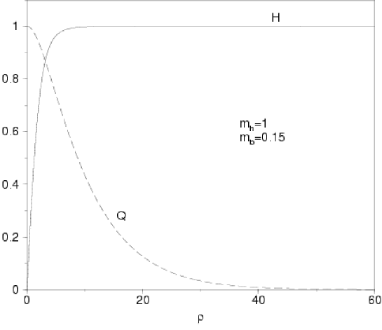
Figure 9.1: The solutions of the field equations for the vortex background. The Higgs field, $H$, takes its vacuum expectation value at infinity and the gauge bosons condensate in the vortex.

The system of Eqs. (9.20) being linear and involving only first order derivatives of the spinor components, a Runge-Kutta numerical method of integration has been used. However, as noted above, since we are interested only in normalizable solutions, it is more convenient to perform the resolution from an arbitrary cutoff at infinity, toward the string core. Let us introduce $\varrho_{\infty}$, the cutoff value on the dimensionless radial distance. From the asymptotic form of Eqs. (9.20) at infinity, and in order to suppress the exponential growth, the spinorial components $\widetilde{\alpha}_{i}$ have to verify

$$\widetilde{\alpha}_{1}(\varrho_{\infty}) = -\frac{\overline{m}}{\Omega m_{\mathrm{h}}}\widetilde{\alpha}_{2}(\varrho_{\infty})+\frac{m_{\mathrm{f}}}{\Omega m_{\mathrm{h}}}\widetilde{\alpha}_{4}(\varrho_{\infty}),$$ (9.34)

$$\widetilde{\alpha}_{3}(\varrho_{\infty}) = -\frac{m_{\mathrm{f}}}{\Omega m_{\mathrm{h}}}\widetilde{\alpha}_{2}(\varrho_{\infty})+\frac{\overline{m}}{\Omega m_{\mathrm{h}}}\widetilde{\alpha}_{4}(\varrho_{\infty}).$$ (9.35)

These conditions constrain two degrees of freedom, and another one is fixed by normalization of the wave functions at $\varrho_{\infty}$. As a result, only one free parameter can be used yet in order to achieve the matching between these well defined solutions and the two normalizable ones near the string core. It will be the case only for particular values of the mass $\overline{m}$. Numerically, the matching is performed in two steps. First, by means of the last free parameter, one of the usually divergent component near the string core is made to vanish at $\varrho=0$. Obviously, this component is chosen among those having a nonzero winding number since, in order to be single valued by rotation around the vortex, it necessarily vanishes at the string core. Once it is performed, the last divergent component at $\varrho=0$ is regularized, its turn, by calculating the mass of the mode $\overline{m}$ leading to a convergent solution. For the range of model parameters previously defined, the numerical computations thus lead to the mass of the trapped wave solutions as well as their components as function of the radial distance to the string core $\widetilde{\alpha}_{i}(\varrho)$.

Numerical results

In what follows, the Higgs winding number is assumed fixed to the value $n=1$, and the range of $c_{\psi_{\mathrm{L}}}$ restricted to $c_{\psi_{\mathrm{L}}}\geq c_{\phi}/2$, the other case being derivable from the symmetric properties discussed above.

The first results concern the “perturbative sector” where the fermion vacuum mass verifies $m_{\mathrm{f}}<m_{\mathrm{h}}$, or equivalently, for a smaller Yukawa coupling constant than the Higgs self-coupling, i.e. $g<\sqrt{\lambda}$. In this case, for reasonable values of the fermion charges, i.e. of the same order of magnitude than the Higgs one $c_{\psi_{\mathrm{L}}}\gtrsim c_{\phi}/2$, only one normalizable massive bound state is found with null winding number $m=0$. As a result, by means of transformations (9.28), there are also symmetric modes for $c_{\psi_{\mathrm{L}}}\leq c_{\phi}/2$, with winding number $m=2$. The dependency of the mode mass $\overline{m}$ with the fermion vacuum mass and charges (i.e. the coupling constants to Higgs and gauge fields) is plotted in Fig. 9.2 and Fig. 9.3. The study has been also extended to the nonperturbative sector where this massive mode thus appears as the lowest massive bound state. First, it is found that the mass of the trapped mode always decreases with respect to the coupling constant, i.e. with the fermion vacuum mass $m_{\mathrm{f}}$. Moreover, for small values of $m_{\mathrm{f}}/m_{\mathrm{h}}$, the derivative of the curve $\overline{m}(m_{\mathrm{f}}/m_{\mathrm{h}})$ vanishes near the origin (see Fig. 9.2). As a result, the mass modes in the full perturbative sector does not depend on the coupling constant to the Higgs field, at first order. On the other hand, Fig. 9.3 shows that the mass of the bound state hardy depends at all on its coupling with the gauge field (i.e. on the charges $c_{\psi_{\mathrm{L}}}$) in the nonperturbative sector, where all the curves have the same asymptotic behavior. Near the origin, the closest $c_{\psi_{\mathrm{L}}}$ is to $c_{\phi}/2$, the higher mode mass $\overline{m}$ is. In the particular limiting case $c_{\psi_{\mathrm{L}}}\sim c_{\phi}/2$, there is no normalizable massive bound state, and as can be seen in Fig. 9.3, already for $c_{\psi_{\mathrm{L}}}/c_{\phi}=2$, the mode mass is close to $m_{\mathrm{f}}$. It is not surprising since, as it was above noted, $c_{\psi_{\mathrm{L}}}=c_{\phi}/2$ is a frontier between two kinds of solutions with different winding numbers, and thus, at this point, the “normalizable” winding numbers are not well defined. Note that this is only true if $m\neq(n+1)/2$ as it is the case here in the perturbative sector with $n=1$ and $m=0$.

Figure 9.2: The mass of the lowest massive bound state, relative to the fermion vacuum mass, plotted as function of the coupling constant to the Higgs field, i.e. the fermion vacuum mass relative to the mass of the Higgs boson.

Figure 9.3: The mass of the lowest massive bound state, relative to the fermion vacuum mass, plotted as function of the coupling constant to the Higgs field, for several values of the fermionic charges. The closest $c_{\psi_{\mathrm{L}}}$ is to $c_{\phi}/2$, the higher mode mass $\overline{m}$ is. In the extreme case $c_{\psi_{\mathrm{L}}}\sim c_{\phi}/2$, $\overline{m}\sim m_{\mathrm{f}}$ there is no longer normalizable massive bound state in the perturbative sector.

The normalized scaled spinorial components $\widetilde{\alpha}(\varrho)$ have been plotted in Fig. 9.4 for the lowest massive bound state, with the normalization

$$\int{\varrho\,{\mathrm{d}}\varrho\,\widetilde{\alpha}_{i}^{{\dagger}}\widetilde{\alpha}_{i}}=1.$$ (9.36)

The corresponding transverse probability density has also been plotted in Fig. 9.4. Note that the massive mode wave function is larger around the string rather on it, as expected for a nonvanishing angular momentum.

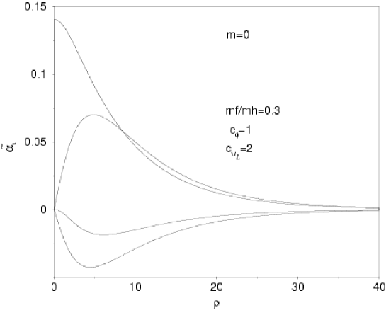
Figure 9.4: The transverse spinorial components of the $\Psi$ field, as functions of the distance to the string core, for the lowest massive bound state. The transverse normalized probability density is also plotted and takes its maximum value nearby the string core, as expected for massive bound states exploring the neighborhood of the core by means of nonvanishing angular momentum. Note that for $m=0$, one spinorial component behaves like a zero mode one, i.e. it condenses in the string core contrary to the others.

The nonperturbative cases with $m_{\mathrm{f}}>m_{\mathrm{h}}$, involve much more massive bound states. First, another mode appears in addition to the previous one, with the same winding number. Because of the fact that $\overline{m}$ decreases with $m_{\mathrm{f}}$ [see Fig. 9.2], for higher values of $m_{\mathrm{f}}$, another mode comes into the normalizable mass range. Since normalizability at infinity requires $\overline{m}<m_{\mathrm{f}}$, the number of massive modes increases with the value of $m_{\mathrm{f}}$. Moreover, there are also solutions involving all the other possible winding numbers. The evolution of the mass spectrum, for winding number $m=0$, and with respect to the coupling constant to the Higgs and gauge fields is plotted in Fig. 9.5. The behavior of each mass is the same as that of the lowest mode previously studied, the new properties resulting only in the appearance of new states for higher values of the fermion vacuum mass $m_{\mathrm{f}}$, as found for two-dimensional Weyl spinors in Ref. [108].

Figure 9.5: The evolution of the mass spectrum for $m=0$ winding number, as function of the coupling constants. Each main branch represents one massive mode whereas the substructures show its evolution with respect to the fermion charge $c_{\psi_{\mathrm{L}}}$. Five values of the fermion charge have been plotted, from $c_{\psi_{\mathrm{L}}}=2$ to $c_{\psi_{\mathrm{L}}}=10$, and the spectrum has been computed only in the nonperturbative sector, since only the lowest mode exists for lower values of $m_{\mathrm{f}}/m_{\mathrm{h}}$ (see Fig. 9.3). As expected, all the modes have mass $\overline{m}$ decreasing with their coupling constant to the Higgs field. Moreover, the substructures show that, for sufficiently large values of $m_{\mathrm{f}}/m_{\mathrm{h}}$, the mode mass is a decreasing function of the charge $c_{\psi_{\mathrm{L}}}$. However, note that this behavior can be inverted for some modes close to their appearance region, as it is the case for the second one.

Physically, the additional massive modes at a given winding number can be interpreted as normalizable eigenstates of the angular momentum operator in the vortex potential, with higher eigenvalues. From Fig. 9.4 and Fig. 9.6, one can see that for each value of $m$, the lowest massive state is confined around the string with a transverse probability density showing only one peak whereas the higher massive modes have transverse probability density profiles with an increasing number of maxima, as can be seen in Fig. 9.7. In fact, as for the structure of atomic spectra, the two spatial degrees of freedom of the attractive potential certainly lead to two quantum numbers labeling the observable eigenstates, one of them being clearly $m$, and the other appearing through the number of zeros of the spinorial components, or, equivalently, the number of maxima of the associated transverse probability density.

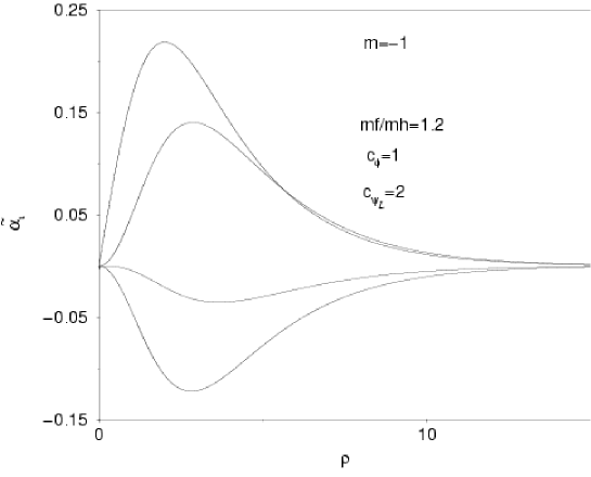
Figure 9.6: The transverse spinorial components of the $\Psi$ field, plotted as functions of the distance to the string core, for the $m=-1$ lowest massive bound state. The transverse normalized probability density is also plotted and vanishes in the string core. In this case, all components of the spinor wind around the string and the corresponding mode is thus centrifugally confined in a shell nearby the core, as expected for a nonzero angular momentum eigenstate.

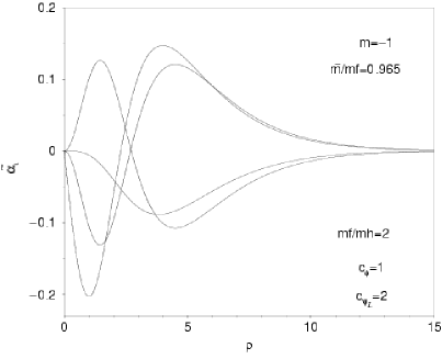
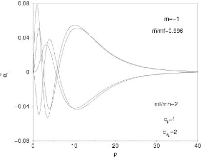
Figure 9.7: The components of the $\Psi$ field as function of the radial distance, and the corresponding transverse probability densities. The curves have been computed for $m=-1$ winding number, and for two additional incoming modes in the nonperturbative sector. As expected, interferences fringes appear from the nonzero angular momentum eigenvalues of these modes.

The massive modes with higher winding numbers behave in the same way. However, they exist only for nonzero values of the coupling constant $m_{\mathrm{f}}/m_{\mathrm{h}}$, this one increasing with the value of the winding number $m$. The scaled spinorial components and the transverse normalized probability density of the lowest massive bound state with next $m=-1$ winding number are plotted in Fig. 9.6. They are found to be normalizable for coupling constant $m_{\mathrm{f}}/m_{\mathrm{h}}\gtrsim 0.5$ when $c_{\psi_{\mathrm{L}}}/c_{\phi}=2$, as can be seen in Fig. 9.8. Contrary to the $m=0$ lowest massive state, all spinorial components wind around the string, and the transverse probability of finding such a mode vanishes in the string core, as expected for a nonzero angular momentum eigenstate. Obviously, this is also true for all higher values of $m$, as for the $m=-2$ massive mode which appears to be normalizable for $m_{\mathrm{f}}/m_{\mathrm{h}}\gtrsim 1.2$.

Figure 9.8: The mass of the $m=-1$ lowest massive bound state, relative to the fermion vacuum mass, with respect to the coupling constant to the Higgs field. Note that the mode does not exist in the perturbative sector.

It is clear from the numerical results that the fermions can be trapped in the string in the form of massive bound states, for a wide range of model parameters. The only exception takes place for fermion charges close to the particular value $c_{\psi_{\mathrm{L}}}=c_{\phi}/2$ where there is no normalizable massive bound state in the perturbative sector. Note, again, that all the previous results are also relevant for the massive modes with symmetric winding numbers $\widehat{m}=n+1-m$, as well as for the ${\mathcal{X}}$ spinor field and for the antiparticle states of both $\Psi$ and ${\mathcal{X}}$ fermions.

9.4 Fock space for massive modes

The existence of massive trapped waves requires that the quantum state space [303] be enlarged to include them. For each normalizable mode with mass $\overline{m}$, a two-dimensional Fock space can be constructed by spinor field expansion over the relevant massive plane waves. The full quantum theory can therefore be obtained from tensorial product of the different Fock spaces belonging to their own mass representation, together with the Fock space associated with the zero modes [303]. As a first step toward a full theory, we will only consider the plane waves associated with one massive mode of mass $\overline{m}$.

9.4.1 Quantum field operators

Quantization is performed through the canonical procedure by defining creation and annihilation operators satisfying anticommutation rules. However, the particular structure of the trapped massive waves yields relationships between longitudinal quantum operators with nontrivial transverse dependencies.

Fourier transform

In the previous section, it was shown that the fermions could propagate along the string direction with given mass $\overline{m}$ belonging to the spectrum. From Eq. (9.17), setting

$$\Psi_{\mathrm{p}}^{(+)}=u_{\psi}(k,r,\theta)\,{\mathrm{e}}^{i(\omega t-kz)}, \Psi_{\mathrm{p}}^{(-)}=v_{\psi}(k,r,\theta)\,{\mathrm{e}}^{-i(\omega t-kz)},$$ (9.37)

with

$$\omega=\sqrt{\overline{m}^{2}+k^{2}},$$ (9.38)

and using the symmetry properties shown in Sec. (9.3.2), the transverse parts of the massive trapped waves for particle and antiparticle states can be written as

$$\begin{array}[]{ccccc}u_{\psi}(k,x_{\perp})&=&\left(\begin{array}[]{c}\sqrt{\omega+k}\,\overline{\alpha}_{1}(r)\,{\mathrm{e}}^{-im\theta}\\ i\sqrt{\omega-k}\,\overline{\alpha}_{2}(r)\,{\mathrm{e}}^{-i(m-1)\theta}\\ \sqrt{\omega-k}\,\overline{\alpha}_{3}(r)\,{\mathrm{e}}^{-i(m-n)\theta}\\ i\sqrt{\omega+k}\,\overline{\alpha}_{4}(r)\,{\mathrm{e}}^{-i(m-n-1)\theta}\end{array}\right),\\ \\ v_{\psi}(k,x_{\perp})&=&\left(\begin{array}[]{c}\sqrt{\omega+k}\,\overline{\alpha}_{1}(r)\,{\mathrm{e}}^{-im\theta}\\ -i\sqrt{\omega-k}\,\overline{\alpha}_{2}(r)\,{\mathrm{e}}^{-i(m-1)\theta}\\ -\sqrt{\omega-k}\,\overline{\alpha}_{3}(r)\,{\mathrm{e}}^{-i(m-n)\theta}\\ i\sqrt{\omega+k}\,\overline{\alpha}_{4}(r)\,{\mathrm{e}}^{-i(m-n-1)\theta}\end{array}\right),\end{array}$$ (9.39)

with the notations

$$x_{\perp}=(r,\theta), \overline{\alpha}=\frac{m_{\mathrm{h}}}{\sqrt{2\pi}}\widetilde{\alpha}.$$ (9.40)

Contrary to the zero mode case, fermions can now propagate in both directions of the string, so that the momentum $k$ of the massive waves can take positive and negative values. As a result, the $\Psi$ field can be Fourier expanded over positive and negative energy states as

$$\Psi=\int{\frac{{\mathrm{d}}k}{2\pi 2\omega}\left[b^{{\dagger}}(k)\,u(k,x_{\perp})\,{\mathrm{e}}^{i(\omega t-kz)}+d(k)\,v(k,x_{\perp})\,{\mathrm{e}}^{-i(\omega t-kz)}\right]},$$ (9.41)

where the subscripts have been omitted. The normalization convention of the Fourier transform is chosen as in the zero modes case [303], i.e.

$$\int{{\mathrm{d}}z\,{\mathrm{e}}^{i(k-k^{\prime})z}}=2\pi\delta(k-k^{\prime}).$$ (9.42)

Obviously, the ${\mathcal{X}}$ field verifies similar relations with the transformation $n\rightarrow-n$, as was noted previously.

Commutation relations

In order to express the Fourier coefficients $b(k)$ and $d^{\dagger}(k)$ as function of the spinor field $\Psi$, let us introduce another unit spinors

$$\begin{array}[]{ccccc}\widehat{u}(k,x_{\perp})&=&\left(\begin{array}[]{c}\sqrt{\omega+k}\,\overline{\alpha}_{3}(r)\,{\mathrm{e}}^{-im\theta}\\ i\sqrt{\omega-k}\,\overline{\alpha}_{4}(r)\,{\mathrm{e}}^{-i(m-1)\theta}\\ \sqrt{\omega-k}\,\overline{\alpha}_{1}(r)\,{\mathrm{e}}^{-i(m-n)\theta}\\ i\sqrt{\omega+k}\,\overline{\alpha}_{2}(r)\,{\mathrm{e}}^{-i(m-n-1)\theta}\end{array}\right),\\ \\ \widehat{v}(k,x_{\perp})&=&\left(\begin{array}[]{c}\sqrt{\omega+k}\,\overline{\alpha}_{3}(r)\,{\mathrm{e}}^{-im\theta}\\ -i\sqrt{\omega-k}\,\overline{\alpha}_{4}(r)\,{\mathrm{e}}^{-i(m-1)\theta}\\ -\sqrt{\omega-k}\,\overline{\alpha}_{1}(r)\,{\mathrm{e}}^{-i(m-n)\theta}\\ i\sqrt{\omega+k}\,\overline{\alpha}_{2}(r)\,{\mathrm{e}}^{-i(m-n-1)\theta}\end{array}\right).\end{array}$$ (9.43)

They clearly verify $\widehat{u}=\gamma^{0}\gamma^{3}\widehat{v}$ and from Eq. (9.39)

$$\begin{array}[]{ccccl}\vspace{4pt}\displaystyle\widehat{u}^{\dagger}(k)u(k)&=&\widehat{v}^{\dagger}(k)v(k)&=&2\omega\,{\overline{\nu}}(r),\\ \vspace{4pt}\displaystyle\widehat{u}(k)^{\dagger}v(-k)&=&\widehat{v}^{\dagger}(k)u(-k)&=&0,\end{array}$$ (9.44)

where the dependency with respect to transverse coordinates have been omitted in order to simplify the notation, and where we introduced the function

$${\overline{\nu}}(r)=\overline{\alpha}_{1}(r)\overline{\alpha}_{3}(r)+\overline{\alpha}_{2}(r)\overline{\alpha}_{4}(r).$$ (9.45)

From Eqs. (9.41), (9.42), and (9.44), the Fourier coefficients are found to be functions of the $\Psi$ field, and read

$$\begin{array}[]{lcl}\vspace{4pt}\displaystyle b^{\dagger}(k)&=&\displaystyle\frac{1}{{\mathcal{N}}}\int{r\,{\mathrm{d}}r\,{\mathrm{d}}\theta\,{\mathrm{d}}z\,{\mathrm{e}}^{-i(\omega t-kz)}\widehat{u}^{\dagger}(k,x_{\perp})\Psi},\\ \vspace{4pt}\displaystyle d(k)&=&\displaystyle\frac{1}{{\mathcal{N}}}\int{r\,{\mathrm{d}}r\,{\mathrm{d}}\theta\,{\mathrm{d}}z\,{\mathrm{e}}^{i(\omega t-kz)}\widehat{v}^{\dagger}(k,x_{\perp})\Psi},\end{array}$$ (9.46)

where we have defined the normalization factor

$${\mathcal{N}}=\int{r\,{\mathrm{d}}r\,{\mathrm{d}}\theta\,{\overline{\nu}}(r)}=\int{\varrho\,{\mathrm{d}}\varrho\,\widetilde{\nu}(\varrho)}$$ (9.47)

Similarly, the expansion of the $\Psi^{\dagger}$ field on the same positive and negative energy solutions leads to the definition of its Fourier coefficients, namely $b(k)$ and $d^{{\dagger}}(k)$. From Eqs. (9.42) and (9.44), they can also be expressed as functions of $\Psi^{\dagger}$, and verify

$$b(k)=[b^{\dagger}(k)]^{\dagger}, d^{\dagger}(k)=[d(k)]^{\dagger}.$$ (9.48)

In order to perform a canonical quantization along the string world sheet, let us postulate the anticommutation rules, at equal times, between the spinor fields

$$\left\{\Psi_{i}(t,\vec{x}),\Psi^{{\dagger}j}(t,\vec{x}^{\prime})\right\} = \delta(z-z^{\prime})\left(\Gamma^{0}\right)_{i}^{j}(x_{\perp},x_{\perp}^{\prime}),$$ (9.49)

where $\Gamma^{0}$ is a matrix with respect to spinor components whose utility will be justified later, and which reads

$$\Gamma^{0}(x_{\perp},x_{\perp}^{\prime}) = \frac{1}{2\overline{m}^{2}}\left(\omega{\mathrm{I}}-k\gamma^{0}\gamma^{3}\right)\left[u(k,x_{\perp})u^{\dagger}(k,x_{\perp}^{\prime})+v(k,x_{\perp})v^{\dagger}(k,x_{\perp}^{\prime})\right].$$ (9.50)

Note that $\Gamma^{0}$ does not depend on $\omega$ and $k$. Explicit calculations show that the first terms involving $\omega$ and $k$ are mixed with $u(k)$ and $v(k)$, and yield Lorentz invariant quantities, such as $\overline{m}$. Moreover, $\Gamma^{0}$ has the following orthonormalization properties

$$\begin{array}[]{lcl}\vspace{4pt}\displaystyle\widehat{u}^{\dagger}(k,x_{\perp})\,\Gamma^{0}(x_{\perp},x_{\perp}^{\prime})\,\widehat{u}(k,x_{\perp}^{\prime})&=&2\omega\,{\overline{\nu}}(r){\overline{\nu}}(r^{\prime})\\ \vspace{4pt}\displaystyle\widehat{u}^{\dagger}(k,x_{\perp})\,\Gamma^{0}(x_{\perp},x_{\perp}^{\prime})\,\widehat{v}(-k,x_{\perp}^{\prime})&=&0,\end{array}$$ (9.51)

and similar relationships are obtained for $\widehat{v}$ by swapping $\widehat{u}$ and $\widehat{v}$.

The anticommutation rules for the $\Psi$ Fourier coefficients are immediately obtained from Eqs. (9.42), (9.46), (9.48), and Eq. (9.49), using the properties of $\Gamma^{0}$ in Eq. (9.51), and read

$$\begin{array}[]{ccccclll}\left\{b(k),b^{\dagger}(k^{\prime})\right\}&=&\left\{d(k),d^{\dagger}(k^{\prime})\right\}&=&2\pi 2\omega\delta(k-k^{\prime}),\end{array}$$ (9.52)

with all the other anticommutators vanishing. As a result, the Fourier coefficients $b^{\dagger}$ and $d^{\dagger}$ behave as well defined creation operators, whereas their complex conjugates, $b$ and $d$, act as annihilation operators of a particle and antiparticle massive state, respectively.

In order to verify the microcausality of the theory and to justify, a posteriori, the ansatz of Eq. (9.49), let us derive the anticommutator between the quantum field operators $\Psi$ and $\Psi^{\dagger}$, at any time. The $\Psi$ expansion in Eq. (9.41) and its complex conjugate yield

$$\left\{\Psi_{i}({\mathbf{x}}),\Psi^{{\dagger}j}({\mathbf{x}}^{\prime})\right\} = \int{\frac{{\mathrm{d}}k\,{\mathrm{d}}k^{\prime}}{(2\pi)^{2}2\omega 2\omega^{\prime}}}\left[\left\{b^{\dagger}(k),b(k^{\prime})\right\}u_{i}(k,x_{\perp})u^{{\dagger}j}(k^{\prime},x_{\perp}^{\prime}){\mathrm{e}}^{i[(\omega t-\omega^{\prime}t^{\prime})-(kz-k^{\prime}z^{\prime})]}\right.$$ (9.53)

$$+ \left.\left\{d(k),d^{\dagger}(k^{\prime})\right\}v_{i}(k,x_{\perp})v^{{\dagger}j}(k^{\prime},x_{\perp}^{\prime}){\mathrm{e}}^{-i[(\omega t-\omega^{\prime}t^{\prime})-(kz-k^{\prime}z^{\prime})]}\right].$$

Using Eq. (9.52), this equation simplifies to involve tensorial products of unit spinors evaluated at the same momentum. It is therefore convenient to introduce two additional matrices, namely $\Gamma^{3}(x_{\perp},x_{\perp}^{\prime})$ and ${\mathcal{M}}(x_{\perp},x_{\perp}^{\prime})$, which verify

$$\begin{array}[]{lcl}\vspace{4pt}\displaystyle u(k,x_{\perp})u^{{\dagger}}(k,x_{\perp}^{\prime})&=&\displaystyle\omega\Gamma^{0}(x_{\perp},x_{\perp}^{\prime})-k\Gamma^{3}(x_{\perp},x_{\perp}^{\prime})-{\mathcal{M}}(x_{\perp},x_{\perp}^{\prime})\\ \vspace{4pt}\displaystyle v(k,x_{\perp})v^{{\dagger}}(k,x_{\perp}^{\prime})&=&\displaystyle\omega\Gamma^{0}(x_{\perp},x_{\perp}^{\prime})-k\Gamma^{3}(x_{\perp},x_{\perp}^{\prime})+{\mathcal{M}}(x_{\perp},x_{\perp}^{\prime}).\end{array}$$ (9.54)

From Eq. (9.39), these matrices are simply related to $\Gamma^{0}$ by

$$\begin{array}[]{lcl}\vspace{4pt}\displaystyle\Gamma^{3}(x_{\perp},x_{\perp}^{\prime})&=&\Gamma^{0}(x_{\perp},x_{\perp}^{\prime})\,\gamma^{3}\gamma^{0},\\ \vspace{4pt}\displaystyle{\mathcal{M}}(x_{\perp},x_{\perp}^{\prime})&=&\displaystyle\Gamma^{0}(x_{\perp},x_{\perp}^{\prime})\,{\mathcal{M}}_{\mathrm{d}}(x_{\perp}^{\prime})\gamma^{0},\end{array}$$ (9.55)

where ${\mathcal{M}}_{\mathrm{d}}(x_{\perp})$ is the diagonal matrix

$${\mathcal{M}}_{\mathrm{d}}(x_{\perp}) = \overline{m}\,{\mathrm{Diag}}\left(\frac{\overline{\alpha}_{3}(r)}{\overline{\alpha}_{1}(r)}{\mathrm{e}}^{-in\theta},\frac{\overline{\alpha}_{4}(r)}{\overline{\alpha}_{2}(r)}{\mathrm{e}}^{-in\theta},\frac{\overline{\alpha}_{1}(r)}{\overline{\alpha}_{3}(r)}{\mathrm{e}}^{in\theta},\frac{\overline{\alpha}_{2}(r)}{\overline{\alpha}_{4}(r)}{\mathrm{e}}^{in\theta}\right).$$ (9.56)

From Eqs. (9.54) and (9.55), the anticommutator (9.53) reduces to

$$\left\{\Psi({\mathbf{x}}),\Psi^{{\dagger}}({\mathbf{x}}^{\prime})\right\} = \left[\Gamma^{0}(x_{\perp},x_{\perp}^{\prime})\,i\partial_{0}+\Gamma^{3}(x_{\perp},x_{\perp}^{\prime})\,i\partial_{3}+{\mathcal{M}}(x_{\perp},x_{\perp}^{\prime})\right]$$ (9.57)

$$\times i\Delta(x_{\parallel}-x_{\parallel}^{\prime}),$$

where $x_{\parallel}=(t,z)$, and $\Delta$ is the well-known Pauli Jordan function which reads

$$i\Delta(x_{\parallel}-x_{\parallel}^{\prime}) = \int{\frac{{\mathrm{d}}k}{2\pi 2\omega}\left[{\mathrm{e}}^{-ik(x_{\parallel}-x_{\parallel}^{\prime})}-{\mathrm{e}}^{ik(x_{\parallel}-x_{\parallel}^{\prime})}\right]},$$ (9.58)

and vanishes outside the light cone. As a result, the quantum fields indeed respect microcausality along the string. The matrices $\Gamma^{\mu}$ appear as the analogues of the matrices $\gamma^{\mu}$ for the Dirac spinors living in the vortex. The two-dimensional quantization along the string is thus not independent of the transverse structure. It is all the more so manifest in the anticommutator expression between $\Psi$ and $\overline{\Psi}$: from Eq. (9.57), and using Eq. (9.55), one gets

$$\left\{\Psi({\mathbf{x}}),\overline{\Psi}({\mathbf{x}}^{\prime})\right\} = \Gamma^{0}(x_{\perp},x_{\perp}^{\prime})\left[i\gamma^{0}\partial_{0}+i\gamma^{3}\partial_{3}+{\mathcal{M}}_{\mathrm{d}}(x_{\perp}^{\prime})\right]\,i\Delta(x_{\parallel}-x_{\parallel}^{\prime}).$$ (9.59)

The matrix $\Gamma^{0}$ now appears clearly as a local transverse normalization of the longitudinal quantum field operators. Note that the mass term also depends on the transverse coordinates due to the nontrivial profile of the Higgs field around the string. Moreover, setting $t=t^{\prime}$ in Eq. (9.57), leads to the postulated anticommutator at equal times (9.49), and therefore justifies the introduction of the $\Gamma^{0}$ term.

Fock states

In the following, $|{\mathcal{P}}\rangle$ will design a Fock state constructed by applying creation operators associated with a massive mode $\overline{m}$, on the relevant string vacuum. Such a state was similarly defined for zero modes in Ref. [303]. From the anticommutators (9.52), a massive $\Psi$ state with momentum $k$ is now normalized according to

$$\langle k^{\prime}|k\rangle=2\pi 2\omega\delta(k-k^{\prime}).$$ (9.60)

Similarly, it will turn out to be convenient to derive the average of the occupation number operator since it will appear in the derivation of the equation of state. From Eq. (9.52), and for a $\Psi$ massive mode, it reads

$$\frac{\langle{\mathcal{P}}|b^{\dagger}(k)b(k^{\prime})|{\mathcal{P}}\rangle}{\langle{\mathcal{P}}|{\mathcal{P}}\rangle}=\frac{2\pi}{L}2\omega 2\pi\sum_{i}\delta(k-k_{i})\delta(k^{\prime}-k_{i}),$$ (9.61)

where the summation runs over all $\Psi$ massive particle states present in the relevant $\overline{m}$ Fock state $|{\mathcal{P}}\rangle$, and $L$ is the physical string length, coming from the $\delta(0)$ regularization by means of Eq. (9.42).

9.4.2 Stress tensor and Hamiltonian

The classical stress tensor can immediately be derived from variation of the full Lagrangian (9.1) with respect to the metric, and the $\Psi$ fermionic part thus reads [303]

$$T_{\psi}^{\mu\nu}=\frac{i}{2}\overline{\Psi}\gamma^{(\mu}\partial^{\nu)}\Psi-\frac{i}{2}\left[\partial^{(\mu}\overline{\Psi}\right]\gamma^{\nu)}\Psi-B^{(\mu}j^{\nu)}_{{}_{\psi}}.$$ (9.62)

Hamiltonian

The quantum operators associated with the classically conserved charges can be obtained by replacing the classical fields by their quantum forms involving creation and annihilation operators. In this way, the Hamiltonian appears, from Noether theorem, as the charge associated with the time component of the energy momentum tensor

$$T^{tt}_{\psi}=i\overline{\Psi}\gamma^{0}\partial_{t}\Psi-i\left(\partial_{t}\overline{\Psi}\right)\gamma^{0}\Psi.$$ (9.63)

Using Eqs. (9.39) and (9.41) in the previous equation, and performing a spatial integration, the Hamiltonian operator reads, after some algebra,

$$P^{t}_{\psi}=\int{\frac{{\mathrm{d}}k}{2\pi 2\omega}}\int{{\mathrm{d}}^{2}x_{\perp}}\left[-b(k)b^{\dagger}(k)+d^{\dagger}(k)d(k)\right]\overline{u}(k,x_{\perp})\gamma^{0}u(k,x_{\perp}).$$ (9.64)

In order to simplify this expression, let us introduce the parameters

$$\overline{\Sigma}_{\mathrm{X}}^{2}=\overline{\alpha}_{2}^{2}+\overline{\alpha}_{3}^{2}, \overline{\Sigma}_{\mathrm{Y}}^{2}=\overline{\alpha}_{1}^{2}+\overline{\alpha}_{4}^{2}.$$ and (9.65)

From Eq. (9.39), the Hamiltonian now reads

$$P^{t}_{\psi}=\int{\frac{{\mathrm{d}}k}{2\pi 2\omega}}\left[-b(k)b^{\dagger}(k)+d^{\dagger}(k)d(k)\right]\left[(\omega-k)||\Sigma_{\mathrm{X}}^{2}||+(\omega+k)||\Sigma_{\mathrm{Y}}^{2}||\right],$$ (9.66)

with

$$||\Sigma^{2}||=\int{r\,{\mathrm{d}}r\,{\mathrm{d}}\theta\,\overline{\Sigma}^{2}}=\int{\varrho\,{\mathrm{d}}\varrho\,\widetilde{\Sigma}^{2}(\varrho)}.$$ (9.67)

Analogous relations also hold for the ${\mathcal{X}}$ field. It is interesting to note that Eq. (9.66) generalizes the expression previously derived in the zero modes case [303], being found again by setting $\omega=-k$ for the $\Psi$ zero modes, or $\omega=k$ for the ${\mathcal{X}}$ ones. The normal ordered Hamiltonian is obtained if one uses the anticommuting normal ordered product for creation and annihilation operators, i.e.

$$:P^{t}_{\psi}:=\int{\frac{{\mathrm{d}}k}{2\pi 2\omega}}\left[b^{\dagger}(k)b(k)+d^{\dagger}(k)d(k)\right]\left[(\omega-k)||\Sigma_{\mathrm{X}}^{2}||+(\omega+k)||\Sigma_{\mathrm{Y}}^{2}||\right].$$ (9.68)

Since $\omega\geq k$, this Hamiltonian is always positive definite and is thus well defined. Note that, as in the zero mode case, such a prescription overlooks the energy density difference between the vacuum on the string and the usual one, but it can be shown to vary as $1/L^{2}$ and therefore goes to zero in the infinite string limit [303, 143, 205].

Effective stress tensor

In order to make contact with the macroscopic formalism [80, 71, 70, 63], it is necessary to express the classically observable quantities with no explicit dependence in the microscopic structure. The relevant two-dimensional fermionic energy momentum tensor can be identified with the full one in Eq. (9.62), once the transverse coordinates have been integrated over. Due to the cylindrical symmetry around the string direction, $z$ say, all nondiagonal components, in a Cartesian basis, involving a transverse coordinate vanish after integration. Moreover, since the fermion fields are normalizable in the transverse plane, the diagonal terms, $T_{\mathcal{F}}^{rr}$ and $T_{\mathcal{F}}^{\theta\theta}$, are also well defined, and by means of local transverse stress tensor conservation, the integrated diagonal components, $T_{\mathcal{F}}^{xx}$ and $T_{\mathcal{F}}^{yy}$, also vanish [280, 279]. As expected, the only relevant terms in the macroscopic formalism are thus $T_{\mathcal{F}}^{\alpha\beta}$ with $\alpha,\beta\in\{t,z\}$, i.e. the ones that live only in the string world sheet. On the other hand, the macroscopic limit of the involved quantum operators is simply obtained by taking their average over the relevant Fock states.

Replacing the quantum fields in Eq. (9.62) by their expansion (9.41), and using Eq. (9.39), one gets the quantum expression of the energy momentum tensor. Averaging the relevant components $T_{\psi}^{\alpha\beta}$ in the Fock state $|{\mathcal{P}}\rangle$, by means of Eqs. (9.39) and (9.61), one obtains

$$\langle:T_{\psi}^{tt}:\rangle_{\mathcal{P}} = \frac{1}{L}\left[\sum_{i}^{N_{\psi}}\overline{u}(k_{i})\gamma^{0}u(k_{i})+\sum_{j}^{\overline{N}_{\psi}}\overline{u}(k_{j})\gamma^{0}u(k_{j})\right],$$ (9.69)

$$\langle:T_{\psi}^{zz}:\rangle_{\mathcal{P}} = \frac{1}{L}\left[\sum_{i}^{N_{\psi}}\frac{k_{i}}{\omega_{i}}\overline{u}(k_{i})\gamma^{3}u(k_{i})+\sum_{j}^{\overline{N}_{\psi}}\frac{k_{j}}{\omega_{j}}\overline{u}(k_{j})\gamma^{3}u(k_{j})\right],$$ (9.70)

$$\langle:T_{\psi}^{tz}:\rangle_{\mathcal{P}} = \frac{1}{2L}\left\{\sum_{i}^{N_{\psi}}\left[\overline{u}(k_{i})\gamma^{3}u(k_{i})+\frac{k_{i}}{\omega_{i}}\overline{u}(k_{i})\gamma^{0}u(k_{i})\right]+(i,N_{\psi})\leftrightarrow(j,\overline{N}_{\psi})\right\},\qquad$$ (9.71)

where the $i$ summations run over the $N_{\psi}$ particle states with momentum $k_{i}$ involved in the Fock state $|{\mathcal{P}}\rangle$, while the $j$ summations take care of the $\overline{N}_{\psi}$ antiparticle states with momentum $k_{j}$, all with mass $\overline{m}$. In order to simplify the notation, the transverse dependence of the unit spinors have not been written, and the averaged operators stand for

$$\langle T^{\alpha\beta}\rangle_{{\mathcal{P}}}=\frac{\langle{\mathcal{P}}|T^{\alpha\beta}|{\mathcal{P}}\rangle}{\langle{\mathcal{P}}|{\mathcal{P}}\rangle}.$$ (9.72)

Similarly, the same relationships can be derived for the ${\mathcal{X}}$ field, by replacing the $\Psi$ unit spinors by the ${\mathcal{X}}$ ones with the correct angular dependence, and certainly, in another mass representation $\overline{m}_{\chi}$. Once the transverse coordinates have been integrated over, Eqs. (9.69), (9.70), and (9.71), lead to the two-dimensional $\Psi$ stress tensor

$$\begin{array}[]{l}\displaystyle\langle\overline{T}_{\psi}^{\alpha\beta}\rangle_{\mathcal{P}}=\\ \\ \left(\begin{array}[]{ccc}\displaystyle E_{\psi_{\mathcal{P}}}||\Sigma_{\mathrm{Y}}^{2}||+\overline{E}_{\psi_{\mathcal{P}}}||\Sigma_{\mathrm{X}}^{2}||&\displaystyle\frac{E_{\psi_{\mathcal{P}}}+P_{\psi_{\mathcal{P}}}}{2}||\Sigma_{\mathrm{Y}}^{2}||-\frac{\overline{E}_{\psi_{\mathcal{P}}}-\overline{P}_{\psi_{\mathcal{P}}}}{2}||\Sigma_{\mathrm{X}}^{2}||\\ \\ \displaystyle\frac{E_{\psi_{\mathcal{P}}}+P_{\psi_{\mathcal{P}}}}{2}||\Sigma_{\mathrm{Y}}^{2}||-\frac{\overline{E}_{\psi_{\mathcal{P}}}-\overline{P}_{\psi_{\mathcal{P}}}}{2}||\Sigma_{\mathrm{X}}^{2}||&\displaystyle P_{\psi_{\mathcal{P}}}||\Sigma_{\mathrm{Y}}^{2}||-\overline{P}_{\psi_{\mathcal{P}}}||\Sigma_{\mathrm{X}}^{2}||\end{array}\right),\end{array}$$ (9.73)

with the notations

$$\begin{array}[]{lcl}\displaystyle E_{\psi_{\mathcal{P}}}&=&\displaystyle\frac{1}{L}\left[\sum_{i}^{N_{\psi}}\left(\omega_{i}+k_{i}\right)+\sum_{j}^{\overline{N}_{\psi}}\left(\omega_{j}+k_{j}\right)\right],\\ \\ \displaystyle\overline{E}_{\psi_{\mathcal{P}}}&=&\displaystyle\frac{1}{L}\left[\sum_{i}^{N_{\psi}}\left(\omega_{i}-k_{i}\right)+\sum_{j}^{\overline{N}_{\psi}}\left(\omega_{j}-k_{j}\right)\right],\\ \\ \displaystyle\end{array}$$ (9.74)

and

$$\begin{array}[]{lcl}P_{\psi_{\mathcal{P}}}&=&\displaystyle\frac{1}{L}\left[\sum_{i}^{N_{\psi}}\frac{k_{i}}{\omega_{i}}\left(\omega_{i}+k_{i}\right)+\sum_{j}^{\overline{N}_{\psi}}\frac{k_{j}}{\omega_{j}}\left(\omega_{j}+k_{j}\right)\right],\\ \\ \displaystyle\overline{P}_{\psi_{\mathcal{P}}}&=&\displaystyle\frac{1}{L}\left[\sum_{i}^{N_{\psi}}\frac{k_{i}}{\omega_{i}}\left(\omega_{i}-k_{i}\right)+\sum_{j}^{\overline{N}_{\psi}}\frac{k_{j}}{\omega_{j}}\left(\omega_{j}-k_{j}\right)\right].\end{array}$$ (9.75)

Recall that the full effective energy momentum tensor also involves the Higgs and gauge fields of the vortex background. Since they essentially describe a Goto-Nambu string [161, 261], their transverse integration yields a traceless diagonal tensor

$$\int{r\,{\mathrm{d}}r\,{\mathrm{d}}\theta\left(T^{tt}_{\mathrm{g}}+T^{tt}_{\mathrm{h}}\right)}=-\int{r\,{\mathrm{d}}r\,{\mathrm{d}}\theta\left(T^{zz}_{\mathrm{g}}+T^{zz}_{\mathrm{h}}\right)}\equiv M^{2}.$$ (9.76)

Note that the full stress tensor may also involve several massive $\Psi$ and ${\mathcal{X}}$ states, with different masses belonging to the spectrum. In this case, there will be as many additional terms in the form of Eq. (9.73), as different massive states there are in the chosen Fock states.

9.4.3 Fermionic currents

The quantum current operators can be derived from their classical expressions (9.14) by using Eq. (9.41), while the corresponding conserved charges are obtained from their spatial integration. By means of Eq. (9.61), the current operator, averaged in the relevant Fock state $|{\mathcal{P}}\rangle$, reads

$$\langle:j^{\alpha}_{\mathcal{F}}:\rangle_{\mathcal{P}} = q\displaystyle{\frac{c_{{\mathcal{F}}_{\mathrm{R}}}+c_{{\mathcal{F}}_{\mathrm{L}}}}{2}}\frac{1}{L}\left(-\sum_{i}^{N_{\mathcal{F}}}\frac{\overline{u}_{i}\gamma^{\alpha}u_{i}}{\omega_{i}}+\sum_{j}^{\overline{N}_{\mathcal{F}}}\frac{\overline{u}_{j}\gamma^{\alpha}u_{j}}{\omega_{j}}\right)$$ (9.77)

$$+ q\displaystyle{\frac{c_{{\mathcal{F}}_{\mathrm{R}}}-c_{{\mathcal{F}}_{\mathrm{L}}}}{2}}\frac{1}{L}\left(-\sum_{i}^{N_{\mathcal{F}}}\frac{\overline{u}_{i}\gamma^{\alpha}\gamma_{5}u_{i}}{\omega_{i}}+\sum_{j}^{\overline{N}_{\mathcal{F}}}\frac{\overline{u}_{j}\gamma^{\alpha}\gamma_{5}u_{j}}{\omega_{j}}\right),$$

with $\alpha\in\{t,z\}$, and once again, the sums run over $\Psi$, or ${\mathcal{X}}$, particle and antiparticle states. The $u_{i}$ are the unit spinors associated with the field dealt with. Concerning the transverse components, due to the properties of the unit spinors $u$ and $v$ in Eq. (9.39), only the orthoradial one does not vanish and reads

$$\langle:j^{\theta}_{\mathcal{F}}:\rangle_{\mathcal{P}} = -q\displaystyle{\frac{c_{{\mathcal{F}}_{\mathrm{R}}}+c_{{\mathcal{F}}_{\mathrm{L}}}}{2}}\frac{1}{L}\left(\sum_{i}^{N_{\mathcal{F}}}\frac{\overline{u}_{i}\gamma^{\theta}u_{i}}{\omega_{i}}+\sum_{j}^{\overline{N}_{\mathcal{F}}}\frac{\overline{u}_{j}\gamma^{\theta}u_{j}}{\omega_{j}}\right)$$ (9.78)

$$- q\displaystyle{\frac{c_{{\mathcal{F}}_{\mathrm{R}}}-c_{{\mathcal{F}}_{\mathrm{L}}}}{2}}\frac{1}{L}\left(\sum_{i}^{N_{\mathcal{F}}}\frac{\overline{u}_{i}\gamma^{\theta}\gamma_{5}u_{i}}{\omega_{i}}+\sum_{j}^{\overline{N}_{\mathcal{F}}}\frac{\overline{u}_{j}\gamma^{\theta}\gamma_{5}u_{j}}{\omega_{j}}\right),$$

whereas $\langle:j_{\mathcal{F}}^{r}:\rangle=0$ due to the bound state nature of the studied currents. As expected, the gauge charges carried by each trapped fermion in the form of massive mode, generate only macroscopic charge and current densities along the string, as was the case for the zero modes [303]. However, the nonvanishing orthoradial component shows that the local charges also wind around the string while propagating in the $z$ direction, as suggested by the above numerical studies. However, this component will be no longer relevant in the macroscopic formalism, since it vanishes in a Cartesian basis, once the transverse coordinates have been integrated over.
Nevertheless, this nonzero angular momentum of the massive modes is found to generate new properties for the longitudinal currents. Let us focus on the vectorial gauge currents generated by one exitation state, with energy $\omega$ and momentum $k$, of a $\Psi$ massive mode, $\overline{m}$ say. From Eq. (9.77), using Eqs. (9.39) and (9.65), the world sheet vectorial charge current reads

$$\langle:j^{0}_{\psi\mathrm{V}}:\rangle_{\varepsilon} = -q\frac{c_{\psi_{\mathrm{R}}}+c_{\psi_{\mathrm{L}}}}{2}\frac{\varepsilon}{L}\left[\left(1+\frac{k}{\omega}\right)\overline{\Sigma}_{\mathrm{Y}}^{2}+\left(1-\frac{k}{\omega}\right)\overline{\Sigma}_{\mathrm{X}}^{2}\right],$$ (9.79)

$$\langle:j^{3}_{\psi\mathrm{V}}:\rangle_{\varepsilon} = -q\frac{c_{\psi_{\mathrm{R}}}+c_{\psi_{\mathrm{L}}}}{2}\frac{\varepsilon}{L}\left[\left(1+\frac{k}{\omega}\right)\overline{\Sigma}_{\mathrm{Y}}^{2}-\left(1-\frac{k}{\omega}\right)\overline{\Sigma}_{\mathrm{X}}^{2}\right],$$ (9.80)

where $\varepsilon=\pm 1$ stands a one particle or antiparticle exitation state. Now, even setting $k=0$ in the previous equations yields a nonvanishing spatial current. Physically, it can be simply interpreted as an anomalous magnetic-like moment of the considered massive mode in its rest frame. Examining Eq. (9.80) shows that it could be null only if $\overline{\Sigma}_{\mathrm{Y}}^{2}(r)=\overline{\Sigma}_{\mathrm{X}}^{2}(r)$, which is generally not satisfied due to the particular shapes of massive spinor components trapped in the string (see Sec. 9.3). These ones being associated with nonzero winding numbers, it is therefore not surprising that, even for a massive stationary state along the string, the nonvanishing charge angular momentum around the string generates such additional magneticlike moment. Note that it does not concern the zero modes, first because they precisely involve vanishing winding numbers [303], and then because for them, there is no defined rest frame due to their vanishing mass. Obviously, this property can be generalized for the axial part of the current, and thus is also valid for the total current of any massive spinor field trapped in the string.

All the above construction of the Fock space and the derivation of the quantum operators associated with the energy momentum tensor and gauge currents remains valid for each $\Psi$ and ${\mathcal{X}}$ massive mode. More precisely, the other masses belonging to the $\Psi$ spectrum verify analogous relationships provided $\overline{m}$ is replaced by the relevant one, as for the unit spinors. In addition, the ${\mathcal{X}}$ massive states require to transform $n\rightarrow-n$ in Eq. (9.56), due to their coupling to the antivortex. At this stage, the averaged values of the stress tensor and currents have been obtained, and therefore allow the derivation of an equation of state, once the Fock states are known.

9.5 Equation of state

The energy per unit length and tension in a given Fock state $|{\mathcal{P}}\rangle$ are basically the eigenvalues associated with timelike and spacelike eigenvectors of the effective two-dimensional full stress tensor. Obviously this one includes the classical Goto-Nambu term resulting of the string forming Higgs and gauge fields [see Eq. (9.76)], with the fermionic part generated by the massive currents [see Eq. (9.73)]. Moreover, in order to describe the string by an adequate macroscopic formalism, it is necessary to choose a quantum statistics for the relevant Fock states, and for energy scales far below the ones where the string was formed, it is reasonable to consider a Fermi-Dirac distribution at zero temperature [303, 283]. In the following, the equation of state is first derived for the lowest massive modes associated with the $\Psi$ and ${\mathcal{X}}$ field, and simplified in the zero-temperature and infinite string limit. As a second step, these derivations are generalized to any number and kind of trapped fermionic mode.

9.5.1 Lowest massive modes

Energy per unit length and tension

In this section, we will only consider the lowest massive modes belonging to the $\Psi$ and ${\mathcal{X}}$ mass spectrums, with masses $\overline{m}_{\psi}$ and $\overline{m}_{\chi}$, respectively. From Eqs. (9.73) and (9.76), the full effective energy momentum tensor reads

$$\langle\overline{T}^{\alpha\beta}\rangle_{\mathcal{P}}=\int{r\,{\mathrm{d}}r\,{\mathrm{d}}\theta\,\left(T^{\alpha\beta}_{\mathrm{g}}+T^{\alpha\beta}_{\mathrm{h}}\right)}+\langle\overline{T}^{\alpha\beta}_{\psi}\rangle_{\mathcal{P}}+\langle\overline{T}^{\alpha\beta}_{\chi}\rangle_{\mathcal{P}},$$ (9.81)

where $\overline{T}^{\alpha\beta}_{\chi}$ takes the same form as $\overline{T}^{\alpha\beta}_{\psi}$ in Eqs. (9.73) and (9.74) once the $\Psi$ relevant parameters have been replaced by the ${\mathcal{X}}$ ones. In the preferred frame where the stress tensor is diagonal, we can identify its timelike and spacelike eigenvalues with energy per unit length $U$ and tension $T$. Upon using Eqs. (9.73), (9.76), and (9.81), these read

$$U_{\mathcal{P}} = M^{2}+\sum_{{\mathcal{F}}\in\{\Psi,{\mathcal{X}}\}}\left(\frac{E_{\mathcal{F}}-P_{\mathcal{F}}}{2}||\Sigma_{\mathrm{Y}{\mathcal{F}}}^{2}||+\frac{\overline{E}_{\mathcal{F}}+\overline{P}_{\mathcal{F}}}{2}||\Sigma_{\mathrm{X}{\mathcal{F}}}^{2}||\right)$$ (9.82)

$$+\quad\left(\sum_{{\mathcal{F}}\in\{\Psi,{\mathcal{X}}\}}\left(E_{\mathcal{F}}+P_{\mathcal{F}}\right)||\Sigma_{\mathrm{Y}{\mathcal{F}}}^{2}||\,\times\,\sum_{{\mathcal{F}}\in\{\Psi,{\mathcal{X}}\}}\left(\overline{E}_{\mathcal{F}}-\overline{P}_{\mathcal{F}}\right)||\Sigma_{\mathrm{X}{\mathcal{F}}}^{2}||\right)^{1/2}\,,$$

for the energy per unit length, and

$$T_{\mathcal{P}} = M^{2}+\sum_{{\mathcal{F}}\in\{\Psi,{\mathcal{X}}\}}\left(\frac{E_{\mathcal{F}}-P_{\mathcal{F}}}{2}||\Sigma_{\mathrm{Y}{\mathcal{F}}}^{2}||+\frac{\overline{E}_{\mathcal{F}}+\overline{P}_{\mathcal{F}}}{2}||\Sigma_{\mathrm{X}{\mathcal{F}}}^{2}||\right)$$ (9.83)

$$-\quad\left(\sum_{{\mathcal{F}}\in\{\Psi,{\mathcal{X}}\}}\left(E_{\mathcal{F}}+P_{\mathcal{F}}\right)||\Sigma_{\mathrm{Y}{\mathcal{F}}}^{2}||\,\times\,\sum_{{\mathcal{F}}\in\{\Psi,{\mathcal{X}}\}}\left(\overline{E}_{\mathcal{F}}-\overline{P}_{\mathcal{F}}\right)||\Sigma_{\mathrm{X}{\mathcal{F}}}^{2}||\right)^{1/2}\,,$$

for the tension. It is interesting to note first that $U_{\mathcal{P}}+T_{\mathcal{P}}\neq 2M^{2}$, and thus the fixed trace equation of state previously found for zero modes [303, 283] is no longer verified by massive modes, as expected since they are no longer eigenstates of the $\gamma^{0}\gamma^{3}$ operator. Moreover, the expression of energy density and tension does not seem to involve the conserved charge current magnitude, which played the role of a state parameter in the case of a scalar condensate in a cosmic string [80, 71, 70, 63, 282]. In fact, as it was the case at zeroth order for the zero modes [303], the charge currents are only involved in the stress tensor through their coupling to the gauge field [see Eq. (9.62)]. At zeroth order, when the back reaction is neglected, the only nonvanishing component of the gauge field is $B_{\theta}$, and it therefore couples only with $j_{\mathcal{F}}^{\theta}$, which vanishes once the transverse coordinates have been integrated over. As a result, it is not surprising that the equation of state does not involve the fermionic currents without back reaction. As a result, it is more natural from quantization to define the occupation numbers of the involved species as state parameters.

Zero-temperature and infinite string limit

Assuming a Fermi-Dirac distribution at zero temperature for the exitation states, the sums involved in Eq. (9.74) run over the successive values of the allowed momentum $k_{i}$ until the Fermi level of the considered species is reached. With periodic boundary conditions on spinor fields, the allowed momentum exitation values are discretized according to

$$k_{n}=\frac{2\pi}{L}n,$$ (9.84)

where $n$ is an integer, playing the role of a quantum exitation number. As a result, in the relevant $\overline{m}$ representation of each field, the exitation energies $\omega_{i}$ are also discrete according to Eq. (9.38), and for the $\Psi$ field, the parameters $E_{\psi}$ and $P_{\psi}$ in Eq. (9.74) simplify to sums of radical function of $n$, with $n$ running from the vacuum to the last filled state. In order to express them as explicit functions of the relevant Fermi level, it is convenient to consider the infinite string limit $L\rightarrow\infty$. In this limit one gets

$$\lim_{L\to\infty}\frac{1}{L}\sum_{i=-N_{\psi}^{-}}^{N_{\psi}^{+}}f(k_{i})=\frac{1}{2\pi}\int_{-2\pi\rho_{\psi}^{-}}^{2\pi\rho_{\psi}^{+}}{\mathrm{d}}k\,f(k),$$ (9.85)

where $\rho_{\psi}^{\pm}=N_{\psi}^{\pm}/L$ are the $\Psi$ up and down mover densities, $N_{\psi}^{+}$, $N_{\psi}^{-}$ standing for the number of $\Psi$ particle moving in the $+z$ or $-z$ directions, respectively. Note that the total number of particles of this kind is thus $N_{\psi}=N_{\psi}^{+}+N_{\psi}^{-}+1$ since there is the additional rest state obtained for $k=0$. After some algebra in Eq. (9.74), using Eq. (9.85), the parameters, for the $\Psi$ field, read

$$E_{\psi} = \frac{\overline{m}^{2}}{4\pi}\left\{\widetilde{\rho}_{\psi}^{+^{2}}-\widetilde{\rho}_{\psi}^{-^{2}}+\left(\widetilde{\rho}_{\psi}^{+}\sqrt{1+\widetilde{\rho}_{\psi}^{+^{2}}}+\widetilde{\rho}_{\psi}^{-}\sqrt{1+\widetilde{\rho}_{\psi}^{-^{2}}}\right)\right.$$ (9.86)

$$+\left.\ln{\left[\left(\sqrt{1+\widetilde{\rho}_{\psi}^{+^{2}}}+\widetilde{\rho}_{\psi}^{+}\right)\left(\sqrt{1+\widetilde{\rho}_{\psi}^{-^{2}}}+\widetilde{\rho}_{\psi}^{-}\right)\right]}\right\}+\left(\widetilde{\rho}_{\psi}^{\pm}\leftrightarrow\overline{\widetilde{\rho}}_{\psi}^{\pm}\right),$$

$$P_{\psi} = \frac{\overline{m}^{2}}{4\pi}\left\{\widetilde{\rho}_{\psi}^{+^{2}}-\widetilde{\rho}_{\psi}^{-^{2}}+\left(\widetilde{\rho}_{\psi}^{+}\sqrt{1+\widetilde{\rho}_{\psi}^{+^{2}}}+\widetilde{\rho}_{\psi}^{-}\sqrt{1+\widetilde{\rho}_{\psi}^{-^{2}}}\right)\right.$$ (9.87)

$$\left.-\ln{\left[\left(\sqrt{1+\widetilde{\rho}_{\psi}^{+^{2}}}+\widetilde{\rho}_{\psi}^{+}\right)\left(\sqrt{1+\widetilde{\rho}_{\psi}^{-^{2}}}+\widetilde{\rho}_{\psi}^{-}\right)\right]}\right\}+\left(\widetilde{\rho}_{\psi}^{\pm}\leftrightarrow\overline{\widetilde{\rho}}_{\psi}^{\pm}\right),$$

where $\widetilde{\rho}_{\psi}$ stands for the dimensionless $\Psi$ mover density

$$\widetilde{\rho}_{\psi}=\frac{2\pi}{\overline{m}}\rho_{\psi},$$ (9.88)

while $\overline{\widetilde{\rho}}_{\psi}$ is defined in the same way for the $\Psi$ antiparticle states. Similarly, the two other parameters $\overline{E}_{\psi}$ and $\overline{P}_{\psi}$ read

$$\overline{E}_{\psi} = \frac{\overline{m}^{2}}{4\pi}\left\{-\widetilde{\rho}_{\psi}^{+^{2}}+\widetilde{\rho}_{\psi}^{-^{2}}+\left(\widetilde{\rho}_{\psi}^{+}\sqrt{1+\widetilde{\rho}_{\psi}^{+^{2}}}+\widetilde{\rho}_{\psi}^{-}\sqrt{1+\widetilde{\rho}_{\psi}^{-^{2}}}\right)\right.$$ (9.89)

$$\left.+\ln{\left[\left(\sqrt{1+\widetilde{\rho}_{\psi}^{+^{2}}}+\widetilde{\rho}_{\psi}^{+}\right)\left(\sqrt{1+\widetilde{\rho}_{\psi}^{-^{2}}}+\widetilde{\rho}_{\psi}^{-}\right)\right]}\right\}+\left(\widetilde{\rho}_{\psi}^{\pm}\leftrightarrow\overline{\widetilde{\rho}}_{\psi}^{\pm}\right),$$

$$\overline{P}_{\psi} = \frac{\overline{m}^{2}}{4\pi}\left\{\widetilde{\rho}_{\psi}^{+^{2}}-\widetilde{\rho}_{\psi}^{-^{2}}-\left(\widetilde{\rho}_{\psi}^{+}\sqrt{1+\widetilde{\rho}_{\psi}^{+^{2}}}+\widetilde{\rho}_{\psi}^{-}\sqrt{1+\widetilde{\rho}_{\psi}^{-^{2}}}\right]\right.$$ (9.90)

$$\left.+\ln{\left[\left(\sqrt{1+\widetilde{\rho}_{\psi}^{+^{2}}}+\widetilde{\rho}_{\psi}^{+}\right)\left(\sqrt{1+\widetilde{\rho}_{\psi}^{-^{2}}}+\widetilde{\rho}_{\psi}^{-}\right)\right]}\right\}+\left(\widetilde{\rho}_{\psi}^{\pm}\leftrightarrow\overline{\widetilde{\rho}}_{\psi}^{\pm}\right).$$

Note that these parameters depend differently on the up and down mover densities as expected for chiral coupling of the fermions to the string forming Higgs field. Recall that in the massless case the zero modes associated with the $\Psi$ and ${\mathcal{X}}$ fields can only propagate in the $-z$ and $+z$ direction respectively [362, 303, 195]. The same relationships also hold for the ${\mathcal{X}}$ field by using the relevant dimensionless mover densities $\widetilde{\rho}^{\pm}_{\chi}$ and $\overline{\widetilde{\rho}}_{\chi}^{\pm}$. Although the equation of state can be derived as a function of these four parameters for each fermion field ${\mathcal{F}}$, it is convenient at this stage to perform some physical simplifications. Contrary to the zero mode case, the coupling between massive particles and antiparticles of the same species ${\mathcal{F}}$ does not vanish along the string. As a result, it is reasonable to consider that the only kind surviving at zero temperature corresponds to the one which was in excess in the plasma in which the string was formed during the phase transition. On the other hand, the energetically favored distribution at zero temperature involves necessarily the same number of ${\mathcal{F}}$ “up” and “down” movers, each filling the accessible states living on each branch of the mass hyperbola (see Fig. 9.9). As a result, in the considered energy scale, it seems reasonable to consider only one state parameter per mass instead of the four initially introduced by quantization, namely $\widetilde{\rho}_{\mathcal{F}}=\widetilde{\rho}_{\mathcal{F}}^{+}=\widetilde{\rho}_{\mathcal{F}}^{-}$, for a plasma dominated by particles, say.

Figure 9.9: The filling of massive states trapped in the string, as expected in the zero-temperature limit, for a particular mass and for one species, $\Psi$ or ${\mathcal{X}}$ say. All antiparticles have disappeared by annihilation with particles during cooling, and the interactions between particles moving in opposite directions, as their coupling to the gauge field, lead to the energetically favored configuration with same number of up and down movers. Obviously, the Fermi level is necessarily below the vacuum mass of the relevant fermion.

Setting these simplifications in Eqs. (9.86) to (9.90), by means of Eqs. (9.82) and (9.83) the energy density and the tension associated with the lowest massive modes now read

$$U = M^{2}+\frac{1}{2\pi}\sum_{{\mathcal{F}}}\overline{m}_{\mathcal{F}}^{2}\ln{\left(\sqrt{1+\widetilde{\rho}_{\mathcal{F}}^{2}}+\widetilde{\rho}_{\mathcal{F}}\right)}$$ (9.91)

$$+\frac{1}{\pi}\,\left(\sum_{\mathcal{F}}\overline{m}_{\mathcal{F}}^{2}\,||\Sigma_{\mathrm{Y}{\mathcal{F}}}^{2}||\,\widetilde{\rho}_{\mathcal{F}}\sqrt{1+\widetilde{\rho}_{\mathcal{F}}^{2}}\,\times\,\sum_{\mathcal{F}}\overline{m}_{\mathcal{F}}^{2}\,||\Sigma_{\mathrm{X}{\mathcal{F}}}^{2}||\,\widetilde{\rho}_{\mathcal{F}}\sqrt{1+\widetilde{\rho}_{\mathcal{F}}^{2}}\right)^{1/2}\,,$$

$$T = M^{2}+\frac{1}{2\pi}\sum_{{\mathcal{F}}}\overline{m}_{\mathcal{F}}^{2}\ln{\left(\sqrt{1+\widetilde{\rho}_{\mathcal{F}}^{2}}+\widetilde{\rho}_{\mathcal{F}}\right)}$$ (9.92)

$$-\frac{1}{\pi}\,\left(\sum_{\mathcal{F}}\overline{m}_{\mathcal{F}}^{2}\,||\Sigma_{\mathrm{Y}{\mathcal{F}}}^{2}||\,\widetilde{\rho}_{\mathcal{F}}\sqrt{1+\widetilde{\rho}_{\mathcal{F}}^{2}}\,\times\,\sum_{\mathcal{F}}\overline{m}_{\mathcal{F}}^{2}\,||\Sigma_{\mathrm{X}{\mathcal{F}}}^{2}||\,\widetilde{\rho}_{\mathcal{F}}\sqrt{1+\widetilde{\rho}_{\mathcal{F}}^{2}}\right)^{1/2}\,.$$

The sum runs over the two lowest massive bound states, each one being associated to the two fermion fields trapped in the vortex, namely $\Psi$ and ${\mathcal{X}}$, and have $\overline{m}_{\psi}$ and $\overline{m}_{\chi}$ masses, respectively. As a result, the equation of state involves two independent parameters, $\widetilde{\rho}_{\psi}$ and $\widetilde{\rho}_{\chi}$, in the zero-temperature and infinite string limit. The energy per unit length and the tension have been plotted in Fig. 9.10, for the lowest massive modes in the nonperturbative sector. The curves are essentially the same in the perturbative sector, but the variations around the Goto-Nambu case $U=T=M^{2}$ are much more damped. For reasonable values of the transverse normalizations, e.g. $||\Sigma_{\mathrm{X}}^{2}||\sim||\Sigma_{\mathrm{Y}}^{2}||\sim 0.5$, and for small values of the dimensionless parameters $\widetilde{\rho}_{\psi}$ and $\widetilde{\rho}_{\chi}$, the energy density is found to grow linearly with $\widetilde{\rho}_{\psi}$ and $\widetilde{\rho}_{\chi}$, whereas the tension varies quadratically. As can be seen in Eq. (9.91), due to the minus sign in $T$, all linear terms in $\widetilde{\rho}$ vanish near origin, whereas it is not the case for the energy density. However, for higher values of the densities, the quadratic terms dominate and both energy density and tension end up being quadratic functions of $\widetilde{\rho}$. On the other hand, according to the macroscopic formalism [80, 71, 70, 63], the string becomes unstable with respect to transverse perturbations when the tension takes on negative values, as in Fig. 9.10 for high densities. Moreover, the decrease of the tension is more damped in the perturbative sector, and the negative values cannot actually be reached for acceptable values of $\widetilde{\rho}$, i.e. $\widetilde{\rho}<m_{\mathrm{f}}/\overline{m}$. As a result, the rapid decrease of the tension with respect to the fermion densities constrains the nonperturbative sector where the string is able to carry massive fermionic currents. For each mass, the higher acceptable value of the $\widetilde{\rho}$ ensuring transverse normalizability is roughly $m_{\mathrm{f}}/\overline{m}$, and from Eq. (9.91), the tension becomes negative at this density for $m_{\mathrm{f}}^{2}\sim 4\pi M^{2}$. Much higher values of $m_{\mathrm{f}}$ will thus yield to empty massive states.

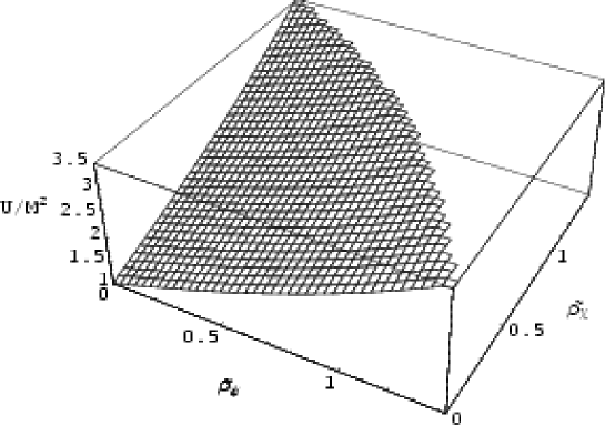
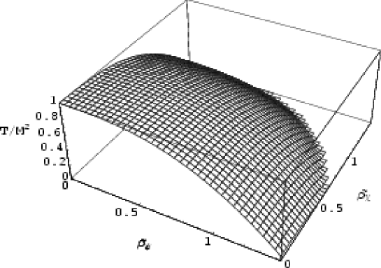
Figure 9.10: The energy per unit length and the tension, in unit of $M^{2}$, for the lowest massive modes alone, plotted as function of the dimensionless effective densities of the two fermion fields, $\widetilde{\rho}_{\psi}$ and $\widetilde{\rho}_{\chi}$. The parameters have been chosen in the nonperturbative sector, with $m_{\mathrm{f}}/m_{\mathrm{h}}\sim 3$ and $\overline{m}_{\chi}\sim\overline{m}_{\psi}\sim 0.6m_{\mathrm{f}}$. Note the linear variation of the energy density near the origin whereas the tension varies quadratically. Moreover, in the allowed range for fermion densities, i.e. less than the fermion vacuum mass, the tension vanishes and the string becomes unstable with respect to transverse perturbations.

As previously noted, the energy density and tension for massive modes no longer verify the fixed trace equation of state found with the zero modes alone. As a result, the longitudinal perturbation propagation speed $c_{\mathrm{L}}^{2}=-dT/dU$ is no longer equal to the speed of light, and it is even no longer well defined since the equation of state involves more than one state parameter. A necessary condition for longitudinal stability can nevertheless be stated by verifying that all the perturbation propagation speeds $-(\partial T/\partial\widetilde{\rho})/(\partial U/\partial\widetilde{\rho})$ obtained from variation of only one state parameter are positive and less than the speed of light. The longitudinal and transverse perturbation propagation speeds, $c^{2}_{\mathrm{L}}$ and $c^{2}_{\mathrm{T}}=T/U$, respectively, have been plotted in Fig. 9.11 in the case where there is only one species trapped as massive mode, $\Psi$ or ${\mathcal{X}}$ say. It is interesting to note that there is a transition between a supersonic regime obtained at low fermion density, and a subsonic at high fermion density. Moreover, the transition density between the two regimes is all the more so high as the coupling constant $m_{\mathrm{f}}/m_{\mathrm{h}}$ is weak. It is not surprising to recover such zero-mode-like subsonic behavior [303, 283] for densities much higher than the rest mass, since in these cases the ultrarelativistic limit applies. On the other hand, since the mass of the massive mode decreases with the coupling constant as in Fig. 9.5, the transition will occur earlier in the nonperturbative sector, as can be seen in Fig. 9.12. Note that the subsonic region is also limited by the maximum allowed values of the massive fermion densities, i.e, $\sim m_{\mathrm{f}}/\overline{m}$, and the regions of transverse instabilities where $c^{2}_{\mathrm{T}}$ becomes negative. Inclusion of the other species does not change significantly these behaviors, the main effect being to lower $c_{\mathrm{T}}^{2}$ with respect to the other fermion density, as can be seen in Fig. 9.10.

Figure 9.11: The squared longitudinal and transverse perturbations propagation speeds for one massive species only, plotted as functions of the dimensionless fermion density $\widetilde{\rho}$, for two values of the coupling constant $m_{\mathrm{f}}/m_{\mathrm{h}}$. Note the transition between subsonic and supersonic behaviors takes place at a cross density, $\widetilde{\rho}_{\times}$ say, which decreases with the coupling constant (see Fig. 9.12).

Figure 9.12: The cross dimensionless density $\widetilde{\rho}_{\times}$, i.e. the dimensionless fermion density for which the transverse and longitudinal perturbation propagation speeds are equal, plotted as function of the coupling constant $m_{\mathrm{f}}/m_{\mathrm{h}}$, for one massive species only. The dashed curve shows the maximum allowed values $m_{\mathrm{f}}/\overline{m}$ of the massive fermion density ensuring transverse normalizability. The transition from supersonic regime to subsonic can thus occurs only in the nonperturbative sector, below this frontier.

The current magnitude can also be derived from the averaged current operators in the zero temperature and infinite string limit. From Eq. (9.77), using Eqs. (9.39) and (9.61), once the transverse coordinates have been integrated over, the world sheet components read

$$\begin{array}[]{lcl}\vspace{4pt}\displaystyle\langle\overline{j}^{0}\rangle&=&\displaystyle-\sum_{\mathcal{F}}\frac{\overline{m}_{\mathcal{F}}}{\pi}\left(qc_{{\mathcal{F}}_{\mathrm{R}}}||\overline{\alpha}_{1}^{2}+\overline{\alpha}_{2}^{2}||+qc_{{\mathcal{F}}_{\mathrm{L}}}||\overline{\alpha}_{4}^{2}+\overline{\alpha}_{3}^{2}||\right)\,\widetilde{\rho}_{\mathcal{F}},\\ \vspace{4pt}\displaystyle\langle\overline{j}^{3}\rangle&=&\displaystyle-\sum_{\mathcal{F}}\frac{\overline{m}_{\mathcal{F}}}{\pi}\left(qc_{{\mathcal{F}}_{\mathrm{R}}}||\overline{\alpha}_{1}^{2}-\overline{\alpha}_{2}^{2}||+qc_{{\mathcal{F}}_{\mathrm{L}}}||\overline{\alpha}_{4}^{2}-\overline{\alpha}_{3}^{2}||\right)\,\widetilde{\rho}_{\mathcal{F}}.\end{array}$$ (9.93)

The current magnitude ${\mathcal{C}}^{2}=\langle\overline{j}^{0}\rangle^{2}-\langle\overline{j}^{3}\rangle^{2}$ therefore reads

$${\mathcal{C}}^{2} = 4\left(\sum_{\mathcal{F}}\frac{\overline{m}_{\mathcal{F}}}{\pi}F_{\mathrm{Y}{\mathcal{F}}}\,\widetilde{\rho}_{\mathcal{F}}\right)\left(\sum_{\mathcal{F}}\frac{\overline{m}_{\mathcal{F}}}{\pi}F_{\mathrm{X}{\mathcal{F}}}\,\widetilde{\rho}_{\mathcal{F}}\right),$$ (9.94)

where $F_{\mathrm{X}{\mathcal{F}}}$ and $F_{\mathrm{Y}{\mathcal{F}}}$ denote the transverse effective charges

$$\begin{array}[]{lcl}\vspace{4pt}\displaystyle F_{\mathrm{Y}{\mathcal{F}}}&=&\displaystyle qc_{{\mathcal{F}}_{\mathrm{R}}}||\overline{\alpha}_{1}^{2}||+qc_{{\mathcal{F}}_{\mathrm{L}}}||\overline{\alpha}_{4}^{2}||\\ \vspace{4pt}\displaystyle F_{\mathrm{X}{\mathcal{F}}}&=&\displaystyle qc_{{\mathcal{F}}_{\mathrm{R}}}||\overline{\alpha}_{2}^{2}||+qc_{{\mathcal{F}}_{\mathrm{L}}}||\overline{\alpha}_{3}^{2}||,\end{array}$$ (9.95)

already introduced for the zero mode currents [303]. In the case of one massive species only, the charge current magnitude simplifies to

$${\mathcal{C}}^{2}=4\frac{\overline{m}^{2}}{\pi^{2}}F_{\mathrm{X}}F_{\mathrm{Y}}\widetilde{\rho}^{2},$$ (9.96)

and thus the sign of ${\mathcal{C}}^{2}$ is only given by the sign of $F_{\mathrm{X}}F_{\mathrm{Y}}$, which is generally positive for reasonable values of the transverse normalizations, e.g. $||\Sigma_{\mathrm{X}}^{2}||\sim||\Sigma_{\mathrm{Y}}^{2}||\sim 0.5$. As a result, the charge current generated by only one massive species is always timelike [108], contrary to the zero mode charge current which was found to be possibly timelike, but also spacelike [303], owing to the allowed exitations of antiparticle zero mode states. As noted above, the antiparticle states cannot exist for massive modes due to the nonvanishing cross section along the string between massive particles and antiparticles. Moreover, and as it was the case for the zero modes, unless there is only one massive species trapped in the string, the magnitude of the charge current is not a sufficient state parameter, contrary to the bosonic current-carrier case [282].

9.5.2 General case

From the numerical approach in Sec. (9.3.2), as soon as the nonperturbative sectors are considered, additional massive bound states become relevant, and it is reasonable to consider that, in the zero-temperature limit, all these accessible massive states will be also be filled. Moreover, the complete description of the string state also requires the inclusion of the zero modes in addition to the massive ones.

Full stress tensor

The effective two-dimensional energy momentum tensor, involving all trapped modes in the cosmic string, can be obtained from Eq. (9.81) by replacing the sum over the two lowest massive modes with the sum over all the accessible masses, plus the zero mode terms previously derived in Ref. [303]. In the preferred frame where the stress tensor is diagonal, after some algebra, the energy density and tension therefore read

$$U = M^{2}+\frac{1}{2\pi}\sum_{{\mathcal{F}},\ell}\overline{m}_{{\mathcal{F}}_{\ell}}^{2}\ln\left(\sqrt{1+\widetilde{\rho}_{{\mathcal{F}}_{\ell}}^{2}}+\widetilde{\rho}_{{\mathcal{F}}_{\ell}}\right)$$ (9.97)

$$+ \frac{1}{\pi}\,\left[\left(4\pi^{2}{\mathcal{R}}_{\chi}^{2}+\sum_{{\mathcal{F}},\ell}\overline{m}_{{\mathcal{F}}_{\ell}}^{2}\,||\Sigma_{\mathrm{Y}{\mathcal{F}}_{\ell}}^{2}||\,\widetilde{\rho}_{{\mathcal{F}}_{\ell}}\sqrt{1+\widetilde{\rho}_{{\mathcal{F}}_{\ell}}^{2}}\right)\right.$$

$$\times\left.\left(4\pi^{2}{\mathcal{R}}_{\psi}^{2}+\sum_{{\mathcal{F}},\ell}\overline{m}_{{\mathcal{F}}_{\ell}}^{2}\,||\Sigma_{\mathrm{X}{\mathcal{F}}_{\ell}}^{2}||\,\widetilde{\rho}_{{\mathcal{F}}_{\ell}}\sqrt{1+\widetilde{\rho}_{{\mathcal{F}}_{\ell}}^{2}}\right)\right]^{1/2}\,,$$

$$T = M^{2}+\frac{1}{2\pi}\sum_{{\mathcal{F}},\ell}\overline{m}_{{\mathcal{F}}_{\ell}}^{2}\ln\left(\sqrt{1+\widetilde{\rho}_{{\mathcal{F}}_{\ell}}^{2}}+\widetilde{\rho}_{\mathcal{F}}\right)$$ (9.98)

$$- \frac{1}{\pi}\,\left[\left(4\pi^{2}{\mathcal{R}}_{\chi}^{2}+\sum_{{\mathcal{F}},\ell}\overline{m}_{{\mathcal{F}}_{\ell}}^{2}\,||\Sigma_{\mathrm{Y}{\mathcal{F}}_{\ell}}^{2}||\,\widetilde{\rho}_{{\mathcal{F}}_{\ell}}\sqrt{1+\widetilde{\rho}_{{\mathcal{F}}_{\ell}}^{2}}\right)\right.$$

$$\times\left.\left(4\pi^{2}{\mathcal{R}}_{\psi}^{2}+\sum_{{\mathcal{F}},\ell}\overline{m}_{{\mathcal{F}}_{\ell}}^{2}\,||\Sigma_{\mathrm{X}{\mathcal{F}}_{\ell}}^{2}||\,\widetilde{\rho}_{{\mathcal{F}}_{\ell}}\sqrt{1+\widetilde{\rho}_{{\mathcal{F}}_{\ell}}^{2}}\right)\right]^{1/2}\,.$$

The sums run over all accessible massive bound states $\ell$ with masses $\overline{m}_{{\mathcal{F}}_{\ell}}$ of each fermion ${\mathcal{F}}$, i.e. $\Psi$ and ${\mathcal{X}}$. The additional parameters ${\mathcal{R}}_{\chi}$ and ${\mathcal{R}}_{\psi}$ are the particle densities trapped in the string in the form of zero modes, for the ${\mathcal{X}}$ and $\Psi$ field, respectively, with same notation as in Ref. [303]. Note that the zero mode contribution can also be obtained from the null mass limit in Eq. (9.91). As a result, the full expression of energy per unit length and tension seems to involve as many state parameters as trapped modes in the string.

Equation of state

As for the lowest massive modes, it is convenient to perform some approximations owing to the energetically favored filling of the involved states, in the zero-temperature limit. In particular, it is reasonable to consider that the nonvanishing cross sections between massive modes, and between zero modes and massive modes, lead to the filling of all the accessible states with energy lower than a Fermi energy, ${\mathcal{E}}_{\mathcal{F}}$ say, for each fermion field ${\mathcal{F}}$. As a result, the energetically favored filling takes place by successive jumps from the lower masses to the highest ones, until the last mass hyperbola with $\overline{m}_{{\mathcal{F}}_{\ell}}\sim{\mathcal{E}}_{\mathcal{F}}$ is reached. Obviously, this filling begins with the zero modes, next with the lowest massive modes and so on. On the other hand, only the particle states are assumed to be relevant because of the assumed annihilation of the antiparticle states, as discussed in Sec. (9.5.1). As a result, the Fermi levels, $\nu_{\mathcal{F}}$ say, can be defined through the zero modes filling only, as the line densities of zero mode exitations trapped in the string (see Fig. 9.13), and thus play the role of state parameters.

Figure 9.13: The accessible states, for the ${\mathcal{X}}$ fermions, in the zero-temperature limit. The zero modes are represented by the chiral line $\omega=k$, while the massive modes appear as mass hyperbolae. The Fermi levels are therefore dependent of the considered energy scale ${\mathcal{E}}$, since the filling is performed by successive jumps from the zero modes to the massive ones, with $\overline{m}_{\ell}\sim{\mathcal{E}}$. As a result, under these approximations, each trapped species leads to only one state parameter which can be identified with the Fermi level of the zero mode exitations, namely $\nu={\mathcal{E}}/2\pi$. Note that the antiparticle states have not been represented due to their assumed annihilation.

According to the so-defined state parameters, the massive exitation densities $\rho_{{\mathcal{F}}_{\ell}}$, in Eqs. (9.97) and (9.98), reduce to

$$\rho_{{\mathcal{F}}_{\ell}} = \left(\nu_{\mathcal{F}}-\frac{\overline{m}_{{\mathcal{F}}_{\ell}}}{2\pi}\right)\Theta\!\!\left(\nu_{\mathcal{F}}-\frac{\overline{m}_{{\mathcal{F}}_{\ell}}}{2\pi}\right),$$ (9.99)

with $\Theta$ function is the Heavyside step function, as expected for energy scales less than the rest mass of the considered massive mode. The zero mode density simply reads

$${\mathcal{R}}_{\mathcal{F}} = \nu_{\mathcal{F}},$$ (9.100)

for zero mode particle states alone. From Eqs. (9.99) and (9.100), and the definition of the dimensionless densities in Eq. (9.88),

$$\widetilde{\rho}_{{\mathcal{F}}_{\ell}}=\frac{2\pi}{\overline{m}_{{\mathcal{F}}_{\ell}}}\rho_{{\mathcal{F}}_{\ell}},$$ (9.101)

the energy per unit length and the tension now depend explicitly of the two state parameters only, namely $\nu_{\psi}$ and $\nu_{\chi}$. By means of Eq. (9.97), the energy density reads

$$U = \displaystyle M^{2}+\frac{1}{2\pi}\sum_{\overline{m}_{{\mathcal{F}}_{\ell}}\leq 2\pi\nu_{\mathcal{F}}}\overline{m}_{{\mathcal{F}}_{\ell}}^{2}\ln{\left[\sqrt{1+\left(\frac{2\pi}{\overline{m}_{{\mathcal{F}}_{\ell}}}\nu_{\mathcal{F}}-1\right)^{2}}+\frac{2\pi}{\overline{m}_{{\mathcal{F}}_{\ell}}}\nu_{\mathcal{F}}-1\right]}$$ (9.102)

$$+ \,\frac{1}{\pi}\,\left[(2\pi\nu_{\chi})^{2}+\sum_{\overline{m}_{{\mathcal{F}}_{\ell}}\leq 2\pi\nu_{\mathcal{F}}}\overline{m}_{{\mathcal{F}}_{\ell}}^{2}\,||\Sigma_{\mathrm{Y}{\mathcal{F}}_{\ell}}^{2}||\,\left(\frac{2\pi}{\overline{m}_{{\mathcal{F}}_{\ell}}}\nu_{\mathcal{F}}-1\right)\sqrt{1+\left(\frac{2\pi}{\overline{m}_{{\mathcal{F}}_{\ell}}}\nu_{\mathcal{F}}-1\right)^{2}}\right]^{1/2}$$

$$\times \,\left[(2\pi\nu_{\psi})^{2}+\sum_{\overline{m}_{{\mathcal{F}}_{\ell}}\leq 2\pi\nu_{\mathcal{F}}}\overline{m}_{{\mathcal{F}}_{\ell}}^{2}\,||\Sigma_{\mathrm{X}{\mathcal{F}}_{\ell}}^{2}||\,\left(\frac{2\pi}{\overline{m}_{{\mathcal{F}}_{\ell}}}\nu_{\mathcal{F}}-1\right)\sqrt{1+\left(\frac{2\pi}{\overline{m}_{{\mathcal{F}}_{\ell}}}\nu_{\mathcal{F}}-1\right)^{2}}\right]^{1/2}\,,$$

while the tension is obtained from Eq. (9.98),

$$T = \displaystyle M^{2}+\frac{1}{2\pi}\sum_{\overline{m}_{{\mathcal{F}}_{\ell}}\leq 2\pi\nu_{\mathcal{F}}}\overline{m}_{{\mathcal{F}}_{\ell}}^{2}\ln{\left[\sqrt{1+\left(\frac{2\pi}{\overline{m}_{{\mathcal{F}}_{\ell}}}\nu_{\mathcal{F}}-1\right)^{2}}+\frac{2\pi}{\overline{m}_{{\mathcal{F}}_{\ell}}}\nu_{\mathcal{F}}-1\right]}$$ (9.103)

$$- \,\frac{1}{\pi}\,\left[(2\pi\nu_{\chi})^{2}+\sum_{\overline{m}_{{\mathcal{F}}_{\ell}}\leq 2\pi\nu_{\mathcal{F}}}\overline{m}_{{\mathcal{F}}_{\ell}}^{2}\,||\Sigma_{\mathrm{Y}{\mathcal{F}}_{\ell}}^{2}||\,\left(\frac{2\pi}{\overline{m}_{{\mathcal{F}}_{\ell}}}\nu_{\mathcal{F}}-1\right)\sqrt{1+\left(\frac{2\pi}{\overline{m}_{{\mathcal{F}}_{\ell}}}\nu_{\mathcal{F}}-1\right)^{2}}\right]^{1/2}$$

$$\times \,\left[(2\pi\nu_{\psi})^{2}+\sum_{\overline{m}_{{\mathcal{F}}_{\ell}}\leq 2\pi\nu_{\mathcal{F}}}\overline{m}_{{\mathcal{F}}_{\ell}}^{2}\,||\Sigma_{\mathrm{X}{\mathcal{F}}_{\ell}}^{2}||\,\left(\frac{2\pi}{\overline{m}_{{\mathcal{F}}_{\ell}}}\nu_{\mathcal{F}}-1\right)\sqrt{1+\left(\frac{2\pi}{\overline{m}_{{\mathcal{F}}_{\ell}}}\nu_{\mathcal{F}}-1\right)^{2}}\right]^{1/2}\,.$$

The full energy per unit length and tension have been plotted in Fig. 9.14 for a configuration including two massive bound states, in addition to the zero mode ones. Due to the zero-temperature limit, for densities smaller than the first accessible mass, the Heavyside functions in Eq. (9.99) vanish, as a result, from Eqs. (9.102) and (9.103) the fixed trace equation of state is recovered [303] with

$$\begin{array}[]{lclclcl}\displaystyle U&=&\displaystyle M^{2}+4\pi\nu_{\chi}\nu_{\psi},&&\displaystyle T&=&\displaystyle M^{2}-4\pi\nu_{\chi}\nu_{\psi}.\end{array}$$ (9.104)

Once the first mass hyperbola is reached, the behaviors of the energy per unit length and tension are clearly modified and become very rapidly dominated by the mass terms, and, as found for the lowest massive modes alone, the energy density begins to grow linearly with respect to the state parameters, whereas the tension decreases quadratically. Actually, the plotted curves in Fig. 9.14 show slope discontinuities each time the phase space is enlarged due to the income of accessible massive bound states (see Fig. 9.13).

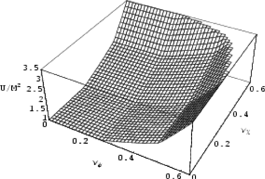
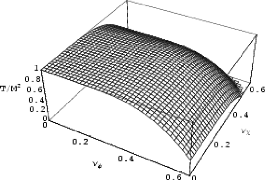
Figure 9.14: The energy per unit length and the tension plotted as function of the two state parameters, i.e. the zero mode densities, in the nonperturbative sector $m_{\mathrm{f}}/m_{\mathrm{h}}\sim 4$. Two additional massive bound states have been considered with respective masses $\overline{m}/m_{\mathrm{f}}\sim 0.4$ and $\overline{m}/m_{\mathrm{f}}\sim 0.6$. In the zero-temperature limit, the filling of the accessible states is performed by successive jumps as soon as the Fermi level reaches one mass hyperbola (see Fig. 9.13). As a result, for the lowest values of the state parameters, only the zero modes are relevant and the fixed trace equation of state, $U+T=2M^{2}$, is verified, then the first and second massive modes are successively reached and become rapidly dominant. As can be seen near the origin, the smooth variations induced by the zero modes appear completely negligible compared to the massive ones. In the perturbative sectors, these behaviors are essentially the same, but the induced variations of the density energy and the tension are all the more small.

On the other hand, it is reasonable to expect competition between the subsonic regimes induced by zero mode currents, or ultrarelativistic massive modes, and the supersonic ones coming from massive currents. In all cases, when the state parameters remain small, only the chiral massless states are accessible and the regime is obviously subsonic, as can be seen in Fig. 9.15. However, the massive mode filling modifies radically this behavior, and as found for the lowest massive modes alone, as soon as a mass hyperbola is reached, the longitudinal perturbations propagation speed falls drastically and ends up being less than the transverse perturbation velocity. There is a rapid transition from the subsonic to the supersonic regime. For higher densities $\nu$, the behavior depends on the coupling constant. More precisely, in the nonperturbative sector, the ultrarelativistic limit can be applied before the energy scales reach the fermion vacuum masses, and thus the subsonic regime is recovered, whereas it is not the case in the perturbative sector, as can be seen in Fig. 9.15.

Figure 9.15: The squared longitudinal and transverse perturbation propagation speeds for a spectrum involving two massive states in addition to the zero mode, plotted as functions of the state parameter $\nu_{\mathcal{F}}$ of one species, the other being fixed to a particular value. The curves have been plotted for two values of the coupling constant to the Higgs field, $m_{\mathrm{f}}/m_{\mathrm{h}}\sim 1$ and $m_{\mathrm{f}}/m_{\mathrm{h}}\sim 4$. Note the successive transitions between subsonic and supersonic behaviors according to the allowed jumps to the mass hyperbolae. However, the fermion vacuum mass limit does not allow the ultrarelativistic limit to take place in the perturbative sector, as it was the case for the lowest massive modes alone. In this case, the string dynamics follows a supersonic regime as soon as the first massive bound state is filled.

Discussion

All these results have been derived without considering the back reaction effects induced by the trapped charge currents along the string [see Eq. (9.93)]. As was already discussed for the zero modes in Ref. [303], these currents yield back reacted gauge field, $B_{t}$ and $B_{z}$, which might modify the vortex background and the fermionic equations of motion. However, such perturbations of the Higgs and orthoradial gauge field profiles (see Fig. 9.1) can be neglected for $B_{t}B^{t}$ and $B_{z}B^{z}$ small compared to the string forming gauge field $B_{\theta}B^{\theta}\sim m_{\mathrm{b}}^{2}$. Using Eqs. (9.40) and (9.93), the dimensionless charge currents associated with one massive bound state, and generating the dimensionless gauge fields $B_{\alpha}/m_{\mathrm{b}}$, roughly read

$$\widetilde{j}^{\alpha}\sim\frac{c_{\mathcal{F}}}{c_{\phi}}\widetilde{\rho}_{\mathcal{F}}\frac{\overline{m}_{\mathcal{F}}}{2\pi^{2}\eta},$$ (9.105)

with $c_{\mathcal{F}}$ the fermion charges, i.e. $c_{{\mathcal{F}}_{\mathrm{R}}}$ or $c_{{\mathcal{F}}_{\mathrm{L}}}$. As a result, the back reaction on the vortex background is negligible as long as $\overline{m}<2\pi^{2}\eta$, which is clearly satisfied in the full perturbative sector. Moreover, since $m_{\mathrm{h}}=\eta\sqrt{\lambda}$, the previous derivations of the equation of state are also valid in the nonperturbative sector provided $\overline{m}<2\pi^{2}m_{\mathrm{h}}/\sqrt{\lambda}$, and thus depend on the values of self-coupling constant of the Higgs field $\lambda$, but also on the mass spectrum. As can be seen in Fig. 9.5, the ratio $\overline{m}/m_{\mathrm{f}}$ decreases with the fermion vacuum mass $m_{\mathrm{f}}$, as a result $\overline{m}/m_{\mathrm{h}}$ increases all the more slowly, which allows to have both $m_{\mathrm{f}}>m_{\mathrm{h}}$ and $\overline{m}<2\pi^{2}m_{\mathrm{h}}/\sqrt{\lambda}$.

Moreover, in order for the new gauge fields $B_{t}$ and $B_{z}$ to not significantly modify the fermionic equations of motion, from Eq. (9.13), they have to verify $qc_{\phi}B_{\alpha}<\omega\sim\overline{m}_{\mathcal{F}}$. As a result, Eq. (9.105), and $B_{\alpha}/m_{\mathrm{b}}\sim\widetilde{j}^{\alpha}$ yield the condition

$$\frac{m_{\mathrm{b}}^{2}}{\eta^{2}}\frac{c_{\mathcal{F}}}{c_{\phi}}<1.$$ (9.106)

As expected, it is essentially the same condition as the one previously derived for the zero modes alone [303]. On the other hand, although the back reaction on the fermionic equations of motion can deeply modify the zero mode currents [302], since the massive bound states are no longer eigenstates of the $\gamma^{0}\gamma^{3}$ operator, it is reasonable to assume that rather than modify their nature and existence significantly, the back reaction gauge fields may only modify their mass spectrum. In this sense, back reaction would indeed be a correction.

9.6 Conclusion

The relevant characteristic features of Dirac fermions trapped in a cosmic string in the form of massive bound states have been study numerically, in the framework of the Witten model, and in the neutral limit. By means of a two-dimensional quantization of the associated spinor fields along the string world sheet, the energy per unit length and the tension of a cosmic string carrying any kind of fermionic current, massive or massless, have been computed, and found to involve as many state parameters as different trapped modes. However, in the zero-temperature limit, only two have been found to be relevant and they can be defined as the density numbers of the chiral zero mode exitations associated with the two fermions $\Psi$ and ${\mathcal{X}}$ coupled to the Higgs field.

As a result, it was shown that the fixed trace equation of state no longer applies, as soon as massive states are filled, i.e. for energy scales larger than the lowest massive mode belonging to the mass spectrum. Moreover, the filling of massive states leads to a rapid transition from the subsonic regime, relevant with massless, or ultrarelativistic currents, to supersonic. Such properties could be relevant in vorton evolution since it has been shown that supersonic regimes generally lead to their classical instabilities [64]. As a result, in the perturbative sectors for which $m_{\mathrm{f}}<m_{\mathrm{h}}$, the protovortons could be essentially produced at energy scales necessarily smaller than the lower mass of the spectrum, where the fermionic currents consist essentially in zero modes. In this way, vortons with fermionic currents could be included in the more general two energy scale models [54]. However, the present conclusions are restricted to parameter domains of the model where the back reaction can be neglected. Although it is reasonable to consider that the back reaction effects may simply modify the massive bound states through their mass values, their influence on zero modes are expected to be much more significant. In particular, the modified zero modes cannot be any longer eigenstates of the $\gamma^{0}\gamma^{3}$ operator [303], so one may conjecture that they acquire an effective mass, leading to massive states potentially instable for cosmic string loops

Acknowledgments

It is a pleasure to thank particularly P. Peter for many fruitful and helpfull discussions. I also wish to acknowledge M. Lemoine, J. Martin, and O. Poujade for advice and various enlightening discussions.

Quatrième partie Cosmologie en dimensions supplémentaires

Chapitre 10 Le modèle de Randall–Sundrum

10.1 Introduction

Les modèles standards de cosmologie et de physique des particules supposent que notre espace-temps possède quatre dimensions. La validité de leurs prédictions (voir chapitres 1 et 2), ainsi que notre perception du monde, semblent donner le statut “d’évidence” à cette hypothèse. Cependant, l’idée qu’il puisse exister des dimensions supplémentaires n’est pas nouvelle. Elle a été initialement motivée par les travaux de Weyl qui tentait d’unifier, de manière géométrique, la gravitation d’Einstein et l’électromagnétisme par l’adjonction de degrés de liberté supplémentaires à l’espace-temps, au travers d’une “covariance conforme” [360]. Dans les années 1920, Kaluza et Klein reprirent cette idée en associant ces degrés de liberté à une dimension spatiale additionnelle compactifiée sur une échelle de longueur $R$ [200, 217]. L’existence physique d’une telle dimension induit cependant des résonances des divers champs pouvant s’y propager, et dont les masses se retrouvent être des multiples entiers de $1/R$. L’absence de ces particules, dites de Kaluza Klein, a finalement repoussé les valeurs admissibles de $R$ aux petites échelles de longueur ($R\ll\,{\mathrm{TeV}}^{-1}$).

Ce sont les théories de cordes fondamentales qui ont ensuite motivé l’existence de dimensions supplémentaires par le fait qu’elles ne peuvent être quantifiées, de manière cohérente, que dans un espace-temps à plus de quatre dimensions [285]. Bien que les échelles de longueur typiques des théories quantiques de gravitation soient voisines de celle de Planck, certaines théories de cordes peuvent néanmoins être étendues jusqu’à des échelles de longueur, $R$, pouvant atteindre le millimètre [181, 182, 18, 17]. Un tel ordre de grandeur permet d’envisager des tests expérimentaux sur l’influence que pourraient avoir ces dimensions cachées, et de ce fait, de contraindre ces théories [189, 237]. Du point de vue de la physique des particules, ces théories ont l’avantage de résoudre les problèmes de hiérarchie des masses. On montre en effet que la compactification des dimensions supplémentaires mène à une échelle de masse effective, dans l’espace-temps usuel, dépendant à la fois de l’échelle de masse typique de la théorie et du volume des extra-dimensions [18, 19, 291]. Le rapport de seize ordres de grandeur existant entre la masse de Planck et l’échelle de brisure électrofaible peut ainsi être, du moins en partie, justifié par la présence de ce volume.

Afin de pouvoir étudier les conséquences physiques de l’existence de dimensions supplémentaires, il est plus commode de construire des modèles phénoménologiques à partir de la théorie des champs. Pour retrouver les propriétés des modèles standards, les champs observés doivent être confinés sur l’hypersurface à trois dimensions dans laquelle nous vivons qui est supposée être immergée dans un espace de dimension supérieure. L’autoconsistence de ces modèles requiert néanmoins de trouver des mécanismes de localisation des divers champs. En particulier, la gravité peut être localisée, comme dans les théories de Kaluza-Klein, par compactification des dimensions supplémentaires [18, 19], mais également par la courbure de l’espace-temps du bulk. Ce dernier cas, introduit par Randall et Sundrum [291], permet d’avoir des dimensions supplémentaires non compactes, et comme nous le verrons dans ce chapitre, on peut y calculer explicitement les écarts induits par les extra-dimensions à la gravité d’Einstein usuelle [291, 146]. Cette gravité modifiée autorise, par ailleurs, l’étude de la viabilité de ces modèles dans le contexte cosmologique [39, 38].

10.2 Gravité linéarisée sur la brane

Le modèle de Randall et Sundrum [291] suppose un espace-temps à cinq dimensions dont la métrique de fond est

$${\mathrm{d}}s^{2}=g_{AB}\,{\mathrm{d}}x^{A}{\mathrm{d}}x^{B}=-{\mathrm{d}}y^{2}+{\mathrm{e}}^{-2\sigma(y)}\eta_{\mu\nu}{\mathrm{d}}x^{\mu}{\mathrm{d}}x^{\nu},$$ (10.1)

où la fonction $\sigma$ est donnée par

$$\sigma(y)=\frac{|y|}{R},$$ (10.2)

$y$ étant la coordonnée dans la cinquième dimension, et $R$ une échelle de distance caractéristique. La théorie de la gravité est de plus supposée être une généralisation de celle d’Einstein à cinq dimensions, c’est-à-dire d’action

$${\mathcal{S}}_{{\mathrm{g}}}=\int\frac{1}{2\kappa_{{}_{5}}^{2}}\left(R-2\Lambda\right)\sqrt{g}\,{\mathrm{d}}^{5}x,$$ (10.3)

avec $g$ le déterminant de la métrique (10.1) et $\kappa_{{}_{5}}^{2}$ la constante de couplage gravitationnelle à cinq dimensions. Elle permet de définir la constante de Newton ${\mathcal{G}}_{{}_{5}}$ et la masse de Planck $m_{{}_{5}}$, dans le bulk, par

$$\kappa_{{}_{5}}^{2}=6\pi^{2}{\mathcal{G}}_{{}_{5}}=\frac{6\pi^{2}}{m_{{}_{5}}^{3}}.$$ (10.4)

Comme nous le verrons dans le chapitre suivant, la métrique (10.1) est solution des équations d’Einstein déduites de l’action (10.3),

$$G^{AB}+\Lambda g^{AB}=\kappa_{{}_{5}}^{2}T_{\infty}^{AB},$$ (10.5)

lorsque la source est une brane dont le tenseur énergie-impulsion, dans la limite d’épaisseur nulle, est donné par [146]

$$T_{\infty}^{\mu\nu}=T_{\infty}g^{\mu\nu}\delta(y).$$ (10.6)

L’existence de la solution statique (10.1) n’est cependant assurée que lorsque la tension $T_{\infty}$ de la brane, et la constante cosmologique $\Lambda$ dans le bulk vérifient les relations

$$T_{\infty}=\frac{1}{\pi^{2}R{\mathcal{G}}_{{}_{5}}}=\frac{m_{{}_{5}}^{3}}{\pi^{2}R},\quad\Lambda=-\frac{6}{R^{2}}.$$ (10.7)

La matière existant sur la brane va modifier cette solution, et en particulier le tenseur métrique $g_{AB}$. En notant $h_{AB}$ ces perturbations, et à partir de l’équation (10.1), on écrit donc la métrique perturbée sous la forme

$${\mathrm{d}}s^{2}=-{\mathrm{d}}y^{2}+{\mathrm{e}}^{-2\sigma(y)}{\mathrm{d}}x^{\mu}{\mathrm{d}}x^{\nu}+h_{AB}\,{\mathrm{d}}x^{A}{\mathrm{d}}x^{B}.$$ (10.8)

Comme dans le cas des équations du mouvement des cordes cosmiques (voir Chap. 4), l’invariance sous les transformations de de coordonnées requiert un choix de jauge. Il est ici commode de se placer dans la jauge dite transverse et sans trace pour $h$ [291], définie par

$$\partial_{\mu}h^{\mu\nu}=\eta_{\mu\nu}h^{\mu\nu}=0.$$ (10.9)

Ce choix de jauge n’est pas encore suffisant, et les degrés de liberté restant doivent être fixés. Cela peut se faire en se plaçant dans la jauge gaussienne normale définie par

$$h_{\mu 4}=h_{44}=0.$$ (10.10)

En reportant (10.8) dans les équations d’Einstein (10.5), et en utilisant les conditions de jauge (10.9) et (10.10), on trouve les équations du mouvement [146],

$$\left({\mathrm{e}}^{2\sigma}\partial_{\mu}^{2}+\partial_{y}^{2}-\frac{4}{R^{2}}\right)h_{\mu\nu}=0.$$ (10.11)

On peut montrer que les conditions de jauge ainsi choisies fixent également la position de la brane en $y=-f^{4}(x^{\mu})$, où $f^{4}$ est une certaine fonction des coordonnées internes à la brane. Cependant, la discontinuité induite par la brane, d’épaisseur nulle, impose des conditions de jonction [146] de la métrique sur celle-ci qu’il est plus commode de fixer en $y=0$. Pour cela, la condition (10.9) doit être relaxée, et il vient, en égalant les parties distributionnelles dans les équations d’Einstein (10.5), toujours pour la métrique (10.8),

$$\left(\partial_{y}+\frac{2}{R}\right)\overline{h}_{\mu\nu}=-\kappa_{{}_{5}}^{2}\left(T_{\mu\nu}-\frac{1}{3}{\mathrm{e}}^{-2\sigma}\eta_{\mu\nu}{T^{\alpha}}_{\alpha}\right),$$ (10.12)

où les perturbations surlignées sont exprimées dans la jauge GN, avec $y=0^{+}$. Afin de pouvoir utiliser cette relation dans les équations du mouvement (10.11), il convient de pouvoir passer d’une jauge à l’autre. D’après l’équation (10.10), la jauge gaussienne normale ne reste vérifiée que pour des changements de coordonnées engendrés par des vecteur $v^{A}$ de la forme

$$v^{4}=f^{4}(x^{\nu}),\quad v^{\mu}=f^{\mu}(x^{\nu})-\frac{R}{2}{\mathrm{e}}^{-2\sigma}\partial^{\mu}f^{4}(x^{\nu}),$$ (10.13)

avec $f^{\mu}$ des fonctions des coordonnées internes à la brane. Les perturbations de la métrique entre les deux jauges sont donc reliées par une transformation également engendrée par les vecteurs $v^{A}$ donnée par [146]

$$h_{\mu\nu}=\overline{h}_{\mu\nu}-R\partial_{\mu}\partial_{\nu}f^{4}-\frac{2}{R}{\mathrm{e}}^{-2\sigma}\eta_{\mu\nu}f^{4}+{\mathrm{e}}^{-2\sigma}\partial_{(\mu}f_{\nu)}.$$ (10.14)

Cette équation permet d’obtenir la condition de jonction (10.12) pour les perturbations $h$, c’est-à-dire,

$$\left(\partial_{y}+\frac{2}{R}\right)h_{\mu\nu}=-\kappa_{{}_{5}}^{5}\left(T_{\mu\nu}-\frac{1}{3}{\mathrm{e}}^{-2\sigma}\eta_{\mu\nu}{T^{\alpha}}_{\alpha}\right)-2\partial_{\mu}\partial_{\nu}f^{4}.$$ (10.15)

En combinant les équations (10.11) et (10.15), les perturbations de la métrique sont finalement solutions de

$$\left[{\mathrm{e}}^{2\sigma}\partial_{\mu}^{2}+\partial_{y}^{2}-\frac{4}{R^{2}}+\frac{4}{R}\delta(y)\right]h_{\mu\nu}=-2\kappa_{{}_{5}}^{5}S_{\mu\nu}\delta(y),$$ (10.16)

avec

$$S_{\mu\nu}=\left(T_{\mu\nu}-\frac{1}{3}{\mathrm{e}}^{-2\sigma}\eta_{\mu\nu}{T^{\alpha}}_{\alpha}\right)+\frac{2}{\kappa_{{}_{5}}^{2}}\partial_{\mu}\partial_{\nu}f^{4}.$$ (10.17)

À l’aide de la fonction de Green retardée $G({\mathbf{x}},y,{\mathbf{x}}^{\prime},y^{\prime})$ associée au membre de gauche de l’équation (10.16), les solutions générales sont données par

$$h_{\mu\nu}=-2\kappa_{{}_{5}}^{5}\int G_{{}_{0}}({\mathbf{x}},{\mathbf{x}}^{\prime})S_{\mu\nu}({\mathbf{x}}^{\prime})\,{\mathrm{d}}^{4}{\mathbf{x}}^{\prime},$$ (10.18)

avec $G_{{}_{0}}$ la fonction de Green $G$ prise sur la brane. Les conditions de jauge transverse (10.9) peuvent maintenant être fixées au travers du terme source $S_{\mu\nu}$. En particulier, l’annulation de sa trace donne l’expression de la coordonnée transverse $f^{4}$. D’après (10.17), il vient

$$\Box f^{4}=\frac{\kappa_{{}_{5}}^{2}}{6}{T^{\alpha}}_{\alpha}.$$ (10.19)

Le calcul explicite de la fonction de Green $G$ montre qu’elle se décompose en deux parties: l’une faisant intervenir des modes de masse nulle, similaires aux gravitons, et l’autre un continuum de modes massifs [146],

$$G({\mathbf{x}},y,{\mathbf{x}}^{\prime},y^{\prime})=\int\frac{{\mathrm{d}}^{4}{\mathbf{k}}}{(2\pi)^{4}}{\mathrm{e}}^{i{\mathbf{k}}({\mathbf{x}}-{\mathbf{x}}^{\prime})}\left[\frac{{\mathrm{e}}^{-2\sigma(y)}{\mathrm{e}}^{-2\sigma(y^{\prime})}/R}{(\omega+i\varepsilon)^{2}-\vec{k}^{{}^{2}}}+\int_{0}^{\infty}\frac{u_{m}(y)u_{m}(y^{\prime})}{(\omega+i\varepsilon)^{2}-\vec{k}^{{}^{2}}-m^{2}}{\mathrm{d}}m\right],$$ (10.20)

où les fonctions propres $u_{m}$ sont données par

$$u_{m}(y)=\sqrt{\frac{mR}{2}}\,\frac{J_{1}(mR)Y_{2}({\mathrm{e}}^{\sigma}mR)-Y_{1}(mR)J_{2}({\mathrm{e}}^{\sigma}mR)}{\sqrt{J_{1}^{2}(mR)+Y_{1}^{2}(mR)}},$$ (10.21)

avec $J_{n}$ et $Y_{n}$ les fonctions de Bessel de première et deuxième espèces, d’ordre $n$.

En choisissant de manière approprié les fonctions $f^{\mu}$, l’équation (10.14) peut être simplifiée, à l’aide de (10.17) et (10.18), en

$$\overline{h}_{\mu\nu}=-2\kappa_{{}_{5}}^{2}\int G_{{}_{0}}({\mathbf{x}},{\mathbf{x}}^{\prime})\left(T_{\mu\nu}-\frac{1}{3}{\mathrm{e}}^{-2\sigma}\eta_{\mu\nu}{T^{\alpha}}_{\alpha}\right){\mathrm{d}}^{4}{\mathbf{x}}^{\prime}+\frac{2}{R}{\mathrm{e}}^{-2\sigma}\eta_{\mu\nu}f^{4},$$ (10.22)

où la fonction $f^{4}$ est solution de l’équation (10.19). La gravité d’Einstein usuelle linéarisée est finalement retrouvée en tronquant la fonction de Green (10.20) à son mode zéro, et il vient

$$\overline{h}_{\mu\nu}=-\frac{2\kappa_{{}_{5}}^{2}}{R}\frac{1}{\nabla^{2}_{\rho}}\left(T_{\mu\nu}-\frac{1}{3}\eta_{\mu\nu}{T^{\alpha}}_{\alpha}\right).$$ (10.23)

Le premier terme dans le membre de droite de cette équation s’identifie naturellement au terme de couplage quadri-dimensionnel en $-16\pi{\mathcal{G}}$, et la constante de gravitation universelle ${\mathcal{G}}$ se trouve reliée à la constante de couplage gravitationnelle dans le bulk par

$$\kappa_{{}_{5}}^{2}=6\pi^{2}{\mathcal{G}}_{{}_{5}}=8\pi{\mathcal{G}}R.$$ (10.24)

Afin d’étudier l’influence du continuum de modes massifs dans la fonction de Green [voir Eq. (10.20)], on peut calculer le potentiel gravitationnel statique dans la brane généré par une masse placée sur celle-ci. En choisissant le tenseur énergie-impulsion de la matière de la forme

$$T_{\mu\nu}=\rho\,u_{\mu}u_{\nu},$$ (10.25)

les $u^{\mu}$ étant les quadrivecteurs vitesses associés, à l’aide des équations (10.19), (10.20) et (10.25), le potentiel newtonnien à l’extérieur de la source, en supposant la symétrie sphérique, est

$$\frac{1}{2}\overline{h}_{00}\simeq\frac{{\mathcal{G}}M}{r}\left(1+\frac{2}{3}\frac{R^{2}}{r^{2}}\right),$$ (10.26)

avec $r=|\vec{x}-\vec{x}^{\,{}^{\prime}\raisebox{2.2pt}[0.0pt][0.0pt]{\tiny}}|$ et $M$ la masse totale $M=\int{\rho}\,{\mathrm{d}}^{3}\vec{x}$. Les modes massifs induisent donc des corrections en $R^{2}/r^{2}$ au potentiel gravitationnel statique, potentiellement détectables aux petites distances telles que $r\simeq R$. Les tests de gravité aux échelles inférieures au millimètre permettent ainsi de fixer une limite supérieure à l’échelle de distance $R$ caractéristique de la cinquième dimension. Notons également que le modèle de Randall-Sundrum permet également de resituer le problème de la hiérarchie des masses. En effet, d’après l’équation (10.24), la masse de Planck dans la brane est donnée par

$$m_{\mathrm{Pl}}^{2}=\frac{1}{8\pi{\mathcal{G}}}=\frac{R}{6\pi^{2}}m_{{}_{5}}^{3}.$$ (10.27)

Pour $R$ voisin du millimètre, la masse de Planck dans le bulk $m_{{}_{5}}$ est abaissée à $10^{8}\,{\mathrm{GeV}}$ pour obtenir $m_{\mathrm{Pl}}\simeq 10^{19}\,{\mathrm{GeV}}$.

Le modèle de Randall-Sundrum donne un cadre phénoménologique, par la théorie des champs, à l’existence d’une dimension supplémentaire dont les effets pourraient être détectés aux petites échelles de longueur. Cependant, bien que le confinement des gravitons de masse nulle soit implicitement assuré, les mécanismes de confinement de la matière ne sont a priori pas inclus dans ce modèle.

10.3 Le confinement des fermions

De la même manière que les gravitons sont piégés sur la brane par la forme de la métrique (10.1), on peut chercher à confiner des fermions du bulk par la gravitation [306, 25]. Comme nous le verrons dans le chapitre suivant, il est possible de décrire des fermions de masse nulle, dans un espace-temps à cinq dimensions, par des spineurs à quatre composantes. Leur lagrangien, en espace-temps courbe de métrique (10.1), est donné par [40]

$${\mathcal{L}}=i\sqrt{g}\,\overline{\Psi}\Gamma^{A}\left[\partial_{A}-\frac{1}{2}\sigma^{\prime}(y){\mathrm{e}}^{-\sigma}\Gamma_{\mu}\Gamma^{4}\right]\Psi,$$ (10.28)

avec $\Gamma^{A}$ les matrices de Dirac en cinq dimensions. On peut maintenant chercher des solutions découplées de la forme

$$\Psi({\mathbf{x}},y)={\mathcal{U}}(y)\psi({\mathbf{x}}),$$ (10.29)

en imposant

$$\gamma^{\mu}\partial_{\mu}\psi=0,$$ (10.30)

pour retrouver un comportement dans la brane similaire à celui d’un fermion quadri-dimensionnel de masse nulle. Dans ce cas, les équations du mouvement déduites du lagrangien (10.28) donnent

$$\left[\partial_{y}-2\sigma^{\prime}(y)\right]{\mathcal{U}}=0,$$ (10.31)

dont la solution est

$${\mathcal{U}}\propto{\mathrm{e}}^{2\sigma}.$$ (10.32)

D’après l’équation (10.2), ces fermions sont complètement délocalisés de la brane. Il est également facile de se convaincre que l’ajout d’un terme de masse dans le lagrangien (10.28) du type $m\overline{\Psi}\Psi$ conduit également à des solutions qui ne sont pas normalisables dans la cinquième dimension. Le modèle de Randall Sundrum ne permet donc pas le confinement des fermions sur la brane.

10.4 Conclusion

La gravité usuelle dans l’espace-temps quadri-dimensionnel peut s’accommoder de l’existence d’une dimension supplémentaire non compacte pourvu que la géométrie dans cette dimension soit de type anti-de Sitter sur une échelle de longueur typiquement inférieure au millimètre. Concernant le secteur de la gravité, de nombreux travaux ont généralisé le modèle de Randall Sundrum à un nombre de dimensions additionnelles supérieur à l’unité [204, 150, 154]. Il est également possible de reproduire dans la brane un espace-temps de type FLRW présentant, comme dans le cas de Minkowski [(voir Eq. 10.1)], des corrections qui pourraient être observables en cosmologie [39, 38]. D’un autre côté, l’autoconsistence phénoménologique de ce modèle est altérée par l’impossibilité de piéger des fermions dans la brane. Une solution consiste à remarquer que, comme les gravitons, il est possible de piéger le mode zéro d’un champ scalaire additionnel [25], et de coupler celui-ci à des fermions. Comme nous le verrons dans le chapitre suivant, si le couplage entre ce champ et les fermions du bulk est suffisamment fort, des fermions de masse nulle peuvent exister sur la brane [25, 306]. Le problème est encore de leur donner une masse: ceci peut être finalement obtenu en supposant qu’il existe un autre champ scalaire sur la brane, de type Higgs, se couplant aux fermions initialement de masse nulle [25]. Ces mécanismes semblent cependant peu naturels vu le nombre de degrés de liberté qu’ils introduisent par rapport au simple modèle initial.

Une autre approche consiste à généraliser les résultats obtenus dans le chapitre 9 concernant les fermions piégés le long des cordes cosmiques. Nous avons vu qu’il existe tout un spectre de fermions, de masses quantifiées, se propageant le long de la corde pourvu que le champ de Higgs auquel ils sont couplés forme un défaut topologique. L’idée est de coupler, à cinq dimensions, des fermions à un unique champ scalaire ayant la propriété de former un mur de domaine qui s’identifie à la brane. Dans le chapitre suivant, publié dans la revue D, nous montrons que la gravité générée par un tel mur de domaine redonne asymptotiquement le modèle de Randall Sundrum, assurant ainsi le confinement des gravitons de masse nulle, et que le couplage des fermions à l’unique champ scalaire conduit à l’apparition de fermions piégés dans la brane ayant un spectre de masse discret [299].

Chapitre 11 Mur de domaine quadri-dimensionnel (article)

Localisation of massive fermions on the brane

Christophe Ringeval¹, Patrick Peter¹ and Jean–Philippe Uzan²

(1) Institut d’Astrophysique de Paris, 98bis Boulevard Arago, F–75014 Paris (France).
(2) Laboratoire de Physique Théorique, CNRS-UMR 8627, Bât. 210,
Université Paris XI, F–91405 Orsay Cedex (France).

We construct an explicit model to describe fermions confined on a four dimensional brane embedded in a five dimensional anti-de Sitter spacetime. We extend previous works to accommodate massive bound states on the brane and exhibit the transverse structure of the fermionic fields. We estimate analytically and calculate numerically the fermion mass spectrum on the brane, which we show to be discrete. The confinement life-time of the bound states is evaluated, and it is shown that existing constraints can be made compatible with the existence of massive fermions trapped on the brane for durations much longer than the age of the Universe.

11.1 Introduction

The idea that our universe may be a hypermembrane in a five dimensional spacetime has received some attention in the last few years after it was realized that gravity could be localized on a three-brane embedded in an anti-de Sitter spacetime [291]. Since then, much work has been done in a cosmological context [39, 100, 90, 38, 219, 315, 140, 241, 306] and there is hope that a consistent (i.e. mathematically self-contained and observationally satisfying) high dimensional model might soon be formulated. For instance, it has been proposed that a model [206, 118] based on such ideas could present itself as an alternative to the inflationary paradigm, although for the time being the controversy as to whether or not such a model might have anything in common with our Universe is still going on [198, 199].

The idea is not new however, but has evolved from the standard Kaluza-Klein approach to that of particle localization on a higher dimensional defect [7, 305, 348, 152]. In particular, it has been shown that massless bulk scalars and gravitons share the property to have a zero mode localized on the brane [25] in the Randall-Sundrum model. Various mechanisms [125, 126, 127, 111, 122, 270, 151, 8] have been invoked according to which it would be possible to confine massless gauge bosons on a brane, so that there is hope to achieve a reasonable model including all the known interactions in a purely four dimensional effective model.

A mechanism permitting localization of massless fermions on a domain wall was described in Refs. [7, 305, 348, 194]. However, although appealing this mechanism might be, it should be emphasized that actual fermions, as seen on an everyday basis in whatever particle physics experiment, are massive, so that a realistic fermionic matter model on the brane must accommodate for such a mass. The question of localization of massive fermions on the brane thus arises naturally, and it is the purpose of this work to provide the transverse brane and fermionic structure that leads to this localization. Up to now, fermions have been confined under the restricting hypothesis that the brane self gravity was negligible [121], or that it was embedded in a Minkowski spacetime with one [180] or two [300] transverse dimensions (see also [262] for the localization of fermion on a string-like defect in five dimension).

Our goal is to transpose the original work of Ref. [300] to the brane context. For that purpose, we realize the brane as a domain wall. Such domain wall configurations in anti-de Sitter space have already been studied [227, 44]. We will assume that five dimensional fermions are Yukawa-coupled to the domain wall forming Higgs field, as in the usual case of cosmic strings. In this respect, our work somehow extends Ref. [121], where the mass term was put by hand, and Ref. [180] where the gravity of the wall was neglected.

We start, in the following section, by recalling the domain wall configuration of a Higgs field in a five dimensional anti-de Sitter spacetime and discuss briefly its properties. In section 11.3, we describe the dynamical equations of fermions coupled to this domain wall in order to show that they obey a Schrödinger-like equation with an effective potential which can trap massive modes on the wall. The asymptotic structure, i.e. deep in the bulk (far from the brane), is not Minkowski space, so that the effective potential felt by the fermions possesses a local minimum at the brane location, but no global minimum, as first pointed out in Ref. [121]. As a consequence, the bound states are metastable and fermions can tunnel to the bulk.

We then provide an analytical approximation of the effective potential, thanks to which we compute analytically, in section 11.4, the mass spectrum of the fermions trapped on the brane. We obtain the mass of the heaviest fermion that can live on the brane and estimate its tunneling rate. This result is compared to a full numerical integration, performed in section 11.5. In a last section, we investigate the parameter space and, after having compared our results to previous ones, we conclude that there exists a wide region in the parameter space for which the fermion masses can be made arbitrary low, i.e. comparable to the observed small values (with respect to the brane characteristic energy scale), while their confinement life-time can be made much larger than the age of the Universe. Such models can therefore be made viable as describing realistic matter on the brane.

11.2 Membrane configuration in AdS₅

We consider the action for a real scalar field $\Phi$ coupled to gravity in a five dimensional spacetime

$$S=\int\left[\frac{1}{2\kappa_{{}_{5}}^{2}}(R-2\Lambda)+\frac{1}{2}g^{AB}\partial_{A}\Phi\partial_{B}\Phi-V(\Phi)\right]\sqrt{g}\,{\mathrm{d}}^{5}x\equiv\int\sqrt{g}\,{\mathrm{d}}^{5}x[{\cal L}_{{}_{\rm grav}}+{\cal L}_{\Lambda}+{\cal L}_{\Phi}]$$ (11.1)

where $g_{AB}$ is the five dimensional metric with signature $(+,-,-,-,-)$, $R$ its Ricci scalar, $\Lambda$ the five dimensional cosmological constant and $\kappa_{{}_{5}}^{2}\equiv 6\pi^{2}{\mathcal{G}}_{{}_{5}}$, ${\mathcal{G}}_{{}_{5}}$ being the five dimensional gravity constant. Capital Latin indices $A,B\ldots$ run from 0 to 4. The potential of the scalar field $\Phi$ is chosen to allow for topological membrane (domain wall like) configurations,

$$V(\Phi)=\frac{\lambda}{8}\left(\Phi^{2}-\eta^{2}\right)^{2},$$ (11.2)

where $\lambda$ is a coupling constant and $\eta=\langle|\Phi|\rangle$ is the magnitude of the scalar field vacuum expectation values (VEV).

Motivated by the brane picture, we choose the metric of the bulk spacetime to be of the warped static form

$${\mathrm{d}}s^{2}=g_{AB}{\mathrm{d}}x^{A}{\mathrm{d}}x^{B}=-{\mathrm{d}}y^{2}+\hbox{e}^{-2\sigma(y)}\eta_{\mu\nu}{\mathrm{d}}x^{\mu}{\mathrm{d}}x^{\nu}=-{\mathrm{d}}y^{2}+g_{\mu\nu}{\mathrm{d}}x^{\mu}{\mathrm{d}}x^{\nu},$$ (11.3)

where $\eta_{\mu\nu}$ is the four dimensional Minkowski metric of signature ($+,-,-,-$), and $y$ the coordinate along the extra-dimension. Greek indices $\mu,\nu\ldots$ run from 0 to 3.

With this metric ansatz, the Einstein tensor components reduce to

$$G_{\mu\nu}=-g_{\mu\nu}(6\sigma^{\prime 2}-3\sigma^{\prime\prime}),\ \ \ G_{yy}=-6\sigma^{\prime 2},$$ (11.4)

where a prime denotes differentiation with respect to $y$. The non-vanishing components of the matter stress-energy tensor

$$T_{AB}\equiv 2{\delta{\cal L}_{\Phi}\over\delta g^{AB}}-g_{AB}{\cal L}_{\Phi}$$ (11.5)

are given by

$$T_{\mu\nu}={1\over 2}g_{\mu\nu}(\Phi^{\prime 2}+2V),\ \ \ \ T_{yy}={1\over 2}(\Phi^{\prime 2}-2V).$$ (11.6)

It follows that the five dimensional Einstein equations

$$G_{AB}+\Lambda g_{AB}=\kappa_{5}^{2}T_{AB}$$ (11.7)

can be cast in the form

$$\frac{3}{\kappa_{{}_{5}}^{2}}\sigma^{\prime\prime} = \Phi^{\prime 2}$$ (11.8)

$$6\sigma^{\prime 2} = \frac{\kappa_{{}_{5}}^{2}}{2}\left(\Phi^{\prime 2}-2V\right)-\Lambda,$$ (11.9)

while the Klein–Gordon equation takes the form

$$\Phi^{\prime\prime}-4\sigma^{\prime}\Phi^{\prime}=\frac{{\mathrm{d}}V}{{\mathrm{d}}\Phi}.$$ (11.10)

Eqs. (11.8-11.10) is a set of three differential equations for two independent variables ($\Phi$ and $\sigma$). Indeed, as can easily be checked, the Klein-Gordon equation stems from the Einstein equations provided $\Phi^{\prime}\neq 0$. To study the domain wall configuration, we choose to solve the first Einstein equation (11.8) together with the Klein-Gordon equation (11.10).

This system of equations must be supplemented with boundary conditions. By definition of the topological defect like configuration, we require that the Higgs field vanishes on the membrane itself, i.e. $\Phi=0$ for $y=0$, while it recovers its VEV in the bulk, so that $\lim_{y\to\pm\infty}\Phi=\pm\eta$. Note that the sign choice made here is arbitrary and corresponds to the so-called kink solution ; the opposite choice (i.e. $\lim_{y\to\pm\infty}\Phi=\mp\eta$) would lead to an anti-kink whose physical properties, as far as we are concerned, are exactly equivalent. As for the metric function $\sigma$, it stems from the requirement that one wants to recover anti-de Sitter asymptotically, so that one demands that $\sigma^{\prime}$ tends to a constant for $y\to\pm\infty$. This constant can be determined using Eq. (11.9), so that $\lim_{y\to\pm\infty}\sigma^{\prime}=\pm\sqrt{-\Lambda/6}$. Note that as $y$ changes sign at the brane location, there is no choice for the sign of the function $\sigma$ in this case. Note also that, as is well known, the static hypothesis implies that the bulk cosmological constant $\Lambda$ must be negative, and therefore the five dimensional spacetime to be anti-de Sitter.

With the convenient dimensionless rescaled variables

$$\varrho\equiv y\sqrt{|\Lambda|},\ \ \ \ H\equiv\frac{\Phi}{\eta},\ \ \ \ \ S\equiv\frac{{\mathrm{d}}\sigma}{{\mathrm{d}}\varrho},$$ (11.11)

the dynamical equations read

$$\dot{S}=\frac{\alpha}{3}\dot{H}^{2},$$ (11.12)

$$\ddot{H}-4S\dot{H}=4\beta H(H^{2}-1),$$ (11.13)

where a dot refers to a derivative with respect to $\varrho$ and the two dimensionless (positive) parameters $\alpha$ and $\beta$ are defined by

$$\alpha\equiv\kappa_{{}_{5}}^{2}\eta^{2},\ \ \ \beta\equiv\frac{\lambda\eta^{2}}{8|\Lambda|}.$$ (11.14)

These parameters are not independent since, for an arbitrary value of $\beta$ say, there is only one value of $\alpha$ for which the boundary condition $S(0)=0$, or equivalently $\lim_{\varrho\to-\infty}S(\varrho)=-1/\sqrt{6}$, is satisfied. This stems from the fact that Eq. (11.12) is a first order equation in $S$, so that only one boundary condition is freely adjustable, and we choose it to be at $\varrho\to+\infty$. Once this choice is made, the value of $S$ on the brane is completely determined, and unless the parameters are given the correct values, it does not vanish. As the solution must be symmetric with respect to the extra dimension coordinate $y$, one must tune the parameters in order to have a meaningfull solution (i.e. for which the metric and its first derivative are continuous at $\varrho=0$). This is reminiscent of the relation that should hold between the brane and bulk cosmological constants [44].

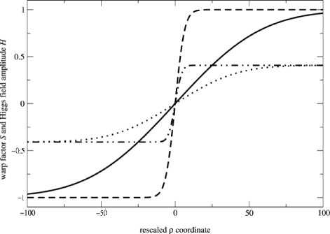
Figure 11.1: The rescaled Higgs field amplitude $H$ (full line for $\beta=0.01$ and dashed line for $\beta=0.1$) and warp factor derivative $S$ (dotted line for $\beta=0.01$ and dot-dashed line for $\beta=0.1$) as functions of the rescaled extra dimension coordinate $\varrho$.

Eqs. (11.12 -11.13) have been solved numerically with the relevant boundary conditions. The field profiles are depicted on Fig. 11.1 for two arbitrary values of the parameter $\beta$.

Figure 11.2: Relation between the dimensionless constants $\alpha$ and $\beta$. The thick curve represent the result of the numerical integration, while the (hardly distinguishable) thin curve is the best analytical fit.

The relation between the parameters $\alpha$ and $\beta$ such that the metric is regular at the brane location is depicted on Fig. 11.2. As can be seen on the figure, it consists essentially in two power laws. For small values of $\beta$, one finds roughly $\alpha\sim 1/\beta$, which becomes exact in the limit $\beta\to 0$, while for large values of $\beta$, one gets $\alpha\sim{4\over 3}\beta^{-1/2}$, which is, again, exact in the limit $\beta\to\infty$. We were able to find the best fit

$$\alpha^{2}={1\over\beta}\left[{1\over\beta}+\left({4\over 3}\right)^{2}\right],$$ (11.15)

which, as can be seen on the figure, is almost exact everywhere. This translates into the relation

$$|\Lambda|={1\over 9}\lambda\eta\left[\sqrt{1+\left({9\kappa_{5}^{2}\eta^{2}\over 8}\right)^{2}}-1\right]$$ (11.16)

between the five dimensional cosmological constant and the microscopic parameters, which corresponds to the usual relations between brane and bulk cosmological constants.

11.3 Localization of fermions on the wall

This section is devoted to the description of the Dirac equation in five dimensions with the domain wall configuration obtained in the previous section.

The minimal representation of spinors in five dimensions can be chosen to be four dimensional [286]. The five dimensional Clifford algebra can then be constructed from the usual four dimensional one by adding the $\gamma_{5}$ matrix to close the algebra. If $\gamma^{\mu}$ design the usual four dimensional Dirac matrices in Minkowski space in the chiral representation, the Dirac matrices in five dimensional Minkowski space, $\Gamma^{A}$, are

$$\Gamma^{\mu}=\gamma^{\mu},\qquad\Gamma^{4}=-i\gamma_{5}$$ (11.17)

and they satisfied the usual Clifford algebra

$$\{\Gamma^{A},\Gamma^{B}\}=2\eta^{AB}$$ (11.18)

where $\eta^{AB}$ stands for the five dimensional Minkowski metric. Since in this representation the Dirac matrices satisfy

$$\Gamma^{5}=i\Gamma^{0}\dots\Gamma^{4}=\mathrm{Id}$$ (11.19)

the five dimensional spinors have neither Weyl nor Majorana represention. It follows that the Dirac Lagrangian in five dimension for fermions coupled to the Higgs domain wall is necessary of the form

$${\mathcal{L}}_{\psi}=\sqrt{g}\left(i\overline{\Psi}\Gamma^{A}{\mathcal{D}}_{A}\Psi-g_{{}_{\rm F}}{\overline{\Psi}}\Phi\Psi\right)=\sqrt{g}\,{\overline{\Psi}}\left[i\hbox{e}^{\sigma(y)}\Gamma^{\mu}{\mathcal{D}}_{\mu}+i\Gamma^{4}\partial_{y}-g_{{}_{\rm F}}\Phi\right]\Psi$$ (11.20)

where the Lorentz covariant derivative with spin connection is [40]

$${\mathcal{D}}_{\mu}\equiv\partial_{\mu}-\frac{1}{2}\sigma^{\prime}(y)\hbox{e}^{-\sigma(y)}\Gamma_{\mu}\Gamma^{4}.$$ (11.21)

We emphasize that the sign of the coupling $g_{{}_{\rm F}}$ of the spinor $\Psi$ to the Higgs field is arbitrary and represents a coupling either to kink or to anti-kink domain wall. For definiteness, we shall consider in what follows only the case of a kink coupling, and thus assume without lack of generality that $g_{{}_{\rm F}}>0$.

The variation of the Lagrangian (11.20) leads to the equation of motion of the spinor field, namely the Dirac equation in five dimensional anti-de Sitter space for a fermionic field coupled to a Higgs field,

$$\left\{i\Gamma^{4}\left[\partial_{y}-2\sigma^{\prime}(y)\right]+i\hbox{e}^{\sigma(y)}\Gamma^{\mu}\partial_{\mu}-g_{{}_{\rm F}}\Phi\right\}\Psi=0.$$ (11.22)

This equation involves the matrix $\gamma_{5}$ (through $\Gamma_{4}$) and it is thus convenient to split the four dimensional right- and left-handed components of the five dimensional spinor and to separate the variables as

$$\Psi(x^{\mu},y)=\left[\frac{1+\gamma_{5}}{2}{\mathcal{U}}_{\rm R}(y)+\frac{1-\gamma_{5}}{2}{\mathcal{U}}_{\rm L}(y)\right]\psi(x^{\mu}),$$ (11.23)

where $\psi(x^{\mu})$ is a four dimensional Dirac spinor, while ${\mathcal{U}}_{\rm R}(y)$ and ${\mathcal{U}}_{\rm L}(y)$ are yet undetermined functions of $y$. In what follows, we want the five dimensional Dirac equation to yield an effective four dimensional massive Dirac equation, with an effective mass $m$ (energy eigenvalue of the bound state). Such a requirement implies that

$$i\gamma^{\mu}\partial_{\mu}\psi=m\psi,$$ (11.24)

or, equivalently, in terms of the right- and left- handed components

$$i\gamma^{\mu}\partial_{\mu}\psi_{\rm R}=m\psi_{\rm L},\qquad i\gamma^{\mu}\partial_{\mu}\psi_{\rm L}=m\psi_{\rm R},$$ (11.25)

where the right- and left-handed components of the four dimensional spinor are defined as

$$\psi_{\rm R}\equiv\frac{1+\gamma_{5}}{2}\psi,\quad\psi_{\rm L}\equiv\frac{1-\gamma_{5}}{2}\psi.$$ (11.26)

Contrary to the case studied in Ref. [121], the mass $m$ is not an arbitrary parameter and will be determined later.

Choosing $\psi_{\rm R}$ and $\psi_{\rm L}$ as the independent variables instead of $\Psi$ and $\overline{\Psi}$, and inserting equation (11.25) into the equation of motion (11.22) while using the splitting ansatz (11.23) yields the differential system for the two functions ${\mathcal{U}}_{{\rm R}/{\rm L}}(y)$,

$$\left[\partial_{y}-2\sigma^{\prime}(y)-g_{{}_{\rm F}}\Phi\right]{\mathcal{U}}_{\rm R}(y) = -m{\mathrm{e}}^{\sigma(y)}{\mathcal{U}}_{\rm L}(y),$$ (11.27)

$$\left[\partial_{y}-2\sigma^{\prime}(y)+g_{{}_{\rm F}}\Phi\right]{\mathcal{U}}_{\rm L}(y) = m{\mathrm{e}}^{\sigma(y)}{\mathcal{U}}_{\rm R}(y).$$ (11.28)

To simplify the notations, it is convenient to introduce the dimensionless rescaled bulk components of the fermions

$$\widetilde{\mathcal{U}}(\varrho)\equiv{\mathrm{e}}^{-\frac{3}{2}\sigma(\varrho)}\frac{{\mathcal{U}}(\varrho)}{|\Lambda|^{1/4}},$$ (11.29)

in terms of which the system (11.27-11.28) takes the form

$$\left[\partial_{\varrho}-\left(\gamma_{{}_{\mathrm{F}}}H+\frac{1}{2}S\right)\right]\,\widetilde{\mathcal{U}}_{\rm R} = -\mu\,{\mathrm{e}}^{\sigma}\widetilde{\mathcal{U}}_{\rm L},$$ (11.30)

$$\left[\partial_{\varrho}+\left(\gamma_{{}_{\mathrm{F}}}H-\frac{1}{2}S\right)\right]\,\widetilde{\mathcal{U}}_{\rm L} = \mu\,{\mathrm{e}}^{\sigma}\widetilde{\mathcal{U}}_{\rm R},$$ (11.31)

with the dimensionless rescaled mass and coupling constant

$$\mu\equiv\frac{m}{\sqrt{|\Lambda|}},\quad\gamma_{{}_{\mathrm{F}}}\equiv\frac{g_{{}_{\rm F}}\eta}{\sqrt{|\Lambda|}}.$$ (11.32)

Let us first concentrate on the special case $\mu=0$. The system (11.30-11.31) then consists in two decoupled differential equations and the zero mode states [292] are recovered. Asymptotically, these functions behave as

$$\widetilde{\mathcal{U}}_{\rm R}(\varrho\rightarrow\pm\infty) \sim {\mathrm{e}}^{\left(\gamma_{{}_{\mathrm{F}}}+\frac{1}{2\sqrt{6}}\right)|\varrho|},$$ (11.33)

$$\widetilde{\mathcal{U}}_{\rm L}(\varrho\rightarrow\pm\infty) \sim {\mathrm{e}}^{-\left(\gamma_{{}_{\mathrm{F}}}-\frac{1}{2\sqrt{6}}\right)|\varrho|}.$$ (11.34)

Thus, only the left-handed solution $\widetilde{\mathcal{U}}_{\rm L}$ may remain bounded [25, 194], and yet provided

$$\gamma_{{}_{\mathrm{F}}}>\frac{1}{2\sqrt{6}}.$$ (11.35)

Indeed, the right-handed zero modes could have been obtained by considering the coupling of fermions to the anti-kink Higgs profile. We thus recover the well-known fact that massless fermions must be single-handed in a brane model, contrary to the ordinary four dimensional field theory in which they simply can.

Let us now focus on the more interesting massive case for which $\mu\not=0$. Then the system (11.30-11.31) can be decoupled by eliminating $\widetilde{\mathcal{U}}_{\rm R}$ say. For that purpose, we differentiate (11.31) with respect to $\varrho$ and express $\partial_{\varrho}\widetilde{\mathcal{U}}_{\rm R}$ using equation (11.30) and $\widetilde{\mathcal{U}}_{\rm R}$ using equation (11.31) again to get

$$\left[\partial^{2}_{\varrho}-2S\,\partial_{\varrho}+\left(\mu^{2}{\mathrm{e}}^{2\sigma}+\frac{3}{4}S^{2}-\gamma_{{}_{\mathrm{F}}}^{2}H^{2}-\gamma_{{}_{\mathrm{F}}}SH-\frac{1}{2}\partial_{\varrho}S+\gamma_{{}_{\mathrm{F}}}\partial_{\varrho}H\right)\right]\widetilde{\mathcal{U}}_{\rm L}=0,$$ (11.36)

$$\widetilde{\mathcal{U}}_{\rm R}-\frac{{\mathrm{e}}^{-\sigma}}{\mu}\left[\partial_{\varrho}+\left(\gamma_{{}_{\mathrm{F}}}H-\frac{1}{2}S\right)\right]\widetilde{\mathcal{U}}_{\rm L}=0.$$ (11.37)

This system is strictly equivalent to the initial system (11.30-11.31) since differentiating Eq. (11.37) and then using Eq. (11.36) gives back Eq. (11.30). It is thus important to keep both equations. Note that the integration of the first equation (11.36) will require two initial conditions but that $\widetilde{\mathcal{U}}_{\rm R}$ will then be completely determined and thus requires no extra constant of integration. As a consequence, it is sufficient to solve the second order equation (11.36) for $\widetilde{\mathcal{U}}_{\rm L}$ in order to fully determine the left- and right-handed bulk fermion profiles.

Eq. (11.36) can be recast into a Schrödinger-like second order differential equation

$$\partial^{2}_{\varrho}\,\widehat{\mathcal{U}}_{\rm L}+\omega^{2}(\varrho)\,\widehat{\mathcal{U}}_{\rm L}=0,$$ (11.38)

where the function $\omega$ is defined by

$$\omega^{2}(\varrho)\equiv\mu^{2}{\mathrm{e}}^{2\sigma(\varrho)}+\partial_{\varrho}\left(\gamma_{{}_{\mathrm{F}}}H+\frac{1}{2}S\right)-\left(\gamma_{{}_{\mathrm{F}}}H+\frac{1}{2}S\right)^{2}$$ (11.39)

with the new function

$$\widehat{\mathcal{U}}(\varrho)\equiv{\mathrm{e}}^{-\sigma(\varrho)}\widetilde{\mathcal{U}}(\varrho).$$ (11.40)

Our aim will now be to find the zero modes of this new equation; as previously discussed, they will be equivalent to the massive bound states we are looking for on the brane.

In order for the fermions to be confined on the brane, the minimum of $\omega^{2}$ needs to be negative to imply an exponential decrease of $\widehat{\mathcal{U}}_{\rm L}$ in the bulk. This is essentially equivalent to the condition (11.35) that was obtained for the case of zero modes. We shall assume henceforth that this condition also holds for massive modes, i.e. that the value of $\gamma_{{}_{\mathrm{F}}}$ necessary to bind massive fermions on the brane is at least that to bind massless ones. Indeed, Eq. (11.39) shows that the minimum of $\omega^{2}$ can only be negative for large values of the parameter $\gamma_{{}_{\mathrm{F}}}$. However, since the first term of (11.39) increases exponentially at large distance from the brane, then, if $\mu\not=0$, $\omega^{2}$ will necessarily become positive. This will yield asymptotic radiative behaviors of the spinor bulk components. Physically, it can be interpreted as a tunneling of the fermions from the brane to the bulk [121]. On the other hand, on the brane, the Higgs field $H$ and the derivative of the warp factor $S$ vanish, so that $\omega^{2}(0)$ is positive. As a result, the fermions can freely propagate in a tiny region around the brane, but certainly only for particular values of $\omega^{2}$ (and thus of $\mu$) satisfying the boundary conditions with the surrounding exponential decreasing regions. The effective potential $V_{{}_{\rm eff}}=-\omega^{2}$, depicted in Fig. 11.3, exhibits a local minimum on the brane and minima at infinity. The modes trapped on the brane are thus expected to have discrete masses $\mu$ on the brane and non-zero probability of tunneling into the bulk.

Figure 11.3: The effective potential $V_{{}_{\rm eff}}=-\omega^{2}$ felt by $\widehat{\mathcal{U}}_{\rm L}$. We chose the parameters $\gamma_{{}_{\mathrm{F}}}=100$ and $\mu=0.5\gamma_{{}_{\mathrm{F}}}$ (an illustrative value, not necessarily leading to a bound state) in the Higgs and gravity background similar to those of Fig. 11.1, and we have assumed, for definiteness, the values $\alpha=1.63$, $\beta=1.23$. The fermions are trapped on the brane where $V_{{}_{\rm eff}}$ is negative and have a non-zero probability of tunneling into the bulk due to combined effects of Higgs and gravity which produce a finite potential barrier.

11.4 Mass spectrum and tunneling rate

Since the Higgs and warp factor profiles are not known analytically, it is a priori impossible to solve Eq. (11.38) analytically. Nevertheless, since the fermions are expected to be trapped in a neighborhood of the brane, we can look for series solutions in $\varrho$.

In § 11.4.1, we give an approximation of the effective potential $V_{{}_{\rm eff}}$ which will then be used to determine the bound states and the mass spectrum in § 11.4.2. We end this section by determining in § 11.4.3 the tunneling rate in this approximation. The validity of this approach is difficult to assess and it will be justified a posteriori on the ground of a full numerical integration of the system in the following section. In the whole section, it is assumed that $\mu>0$.

11.4.1 Approximation of the effective potential

In a neighborhood of the brane we can expand the Higgs and warp factor profiles as

$$H(\varrho) = H_{1}\varrho+H_{3}\varrho^{3}+{\mathcal{O}}(\varrho^{4}),$$ (11.41)

$$S(\varrho) = S_{1}\varrho+S_{3}\varrho^{3}+{\mathcal{O}}(\varrho^{4}),$$ (11.42)

where both the constant and quadratic terms vanish for symmetry reasons. To simplify the analysis, we shall make use of the equations of motion in the form

$$\dot{S}={2\over 3}F(S,H),$$ (11.43)

and

$$\dot{H}=\pm\sqrt{{2\over\alpha}F(S,H)},$$ (11.44)

where the function $F(S,H)$ is defined as

$$F(S,H)\equiv 6S^{2}+\alpha\beta(H^{2}-1)^{2}-1,$$ (11.45)

(recall that $\Lambda<0$).

Plugging the expansions (11.41) and (11.42) into Eqs. (11.43) and (11.44), it follows that the function $F(S,H)$ can be expanded up to third order as

$$F(S,H)\sim\alpha\beta-1+\left(6S_{1}^{2}-2\alpha\beta H_{1}^{2}\right)\varrho^{2}+{\mathcal{O}}(\varrho^{4}).$$ (11.46)

Inserting this expression back into the equations of motion yields the three coefficients

$$S_{1} = \frac{\alpha}{3}H_{1}^{2},$$ (11.47)

$$S_{3} = \frac{4}{9}\alpha H_{1}^{2}\left[\frac{\alpha}{3}H_{1}^{2}-\beta\right],$$ (11.48)

$$H_{3} = \frac{2}{3}H_{1}\left[\frac{\alpha}{3}H_{1}^{2}-\beta\right]$$ (11.49)

in terms of the coefficient $H_{1}$

$$H_{1}\equiv\left.\partial_{\varrho}H\right|_{\varrho=0}=\sqrt{\frac{2}{\alpha}(\alpha\beta-1)}.$$ (11.50)

Then, the frequency $\omega^{2}$ can be expanded as an harmonic oscillator potential

$$\omega^{2}(\varrho)=\omega_{\rm b}^{2}(\varrho)+{\mathcal{O}}(\varrho^{4})\qquad\hbox{with}\qquad\omega^{2}_{\rm b}(\varrho)\equiv\omega_{0}^{2}-\Omega\,\varrho^{2}$$ (11.51)

where $\omega_{0}^{2}$ and $\Omega$ are given by

$$\omega_{0}^{2} \equiv \mu^{2}+\gamma_{{}_{\mathrm{F}}}H_{1}\left(1+\frac{\alpha}{6\gamma_{{}_{\mathrm{F}}}}H_{1}\right)$$ (11.52)

$$\Omega \equiv H_{1}\gamma_{{}_{\mathrm{F}}}^{2}\left[H_{1}+\frac{2}{\gamma_{{}_{\mathrm{F}}}}\left(\beta-\frac{\alpha}{6}H_{1}^{2}\right)+\frac{\alpha}{3\gamma_{{}_{\mathrm{F}}}^{2}}H_{1}\left(2\beta-\mu^{2}-\frac{7\alpha}{12}H_{1}^{2}\right)\right].$$ (11.53)

The function $\omega^{2}$ is well approximated by $\omega_{\rm b}^{2}$ only near the brane and the expansion (11.51) is no longer valid at large distance where the exponential term dominates [see Eq. (11.39)]. Once the fixed asymptotic values of the Higgs and warp factor are reached, the frequency (11.39) behaves as $\omega^{2}\sim\omega^{2}_{\infty}(\varrho)$, with

$$\omega^{2}_{\infty}=\mu^{2}{\mathrm{e}}^{2|\varrho|/\sqrt{6}}-\left(\gamma_{{}_{\mathrm{F}}}+\frac{1}{2\sqrt{6}}\right)^{2}.$$ (11.54)

The analytical estimate of the function $\omega^{2}$ is thus obtained by matching the two limiting asymptotic behaviors (11.51) and (11.54), respectively $\omega_{\rm b}^{2}$ closes to the brane and $\omega^{2}_{\infty}$ far from it, as

$$\omega^{2}(\rho)=\left\{\begin{array}[]{cc}\omega_{\rm b}^{2},&|\rho|<\rho_{{}_{\rm m}}\\ \omega_{\infty}^{2},&|\rho|>\rho_{{}_{\rm m}}\end{array}\right..$$ (11.55)

The dimensionless matching distance $\varrho_{{}_{\rm m}}$ has to be solution of

$$\omega^{2}_{{}_{\rm b}}(\varrho_{{}_{\rm m}})=\omega^{2}_{\infty}(\varrho_{{}_{\rm m}}),$$ (11.56)

in order to get a continuous function. Note that, because of the symmetry on both sides of the wall, we can assume $\varrho_{{}_{\rm m}}>0$ without lack of generality. For large values of $\gamma_{{}_{\mathrm{F}}}$, and using Eq. (11.53), we get

$$\sqrt{\Omega}\sim\gamma_{{}_{\mathrm{F}}}H_{1},$$ (11.57)

leading to

$$\varrho_{{}_{\rm m}}\sim\frac{1}{H_{1}}.$$ (11.58)

As it turns out, the faster the asymptotic solution is reached, the better the approximation works. This is the case in particular for $H_{1}>1$,

The exact (numerically integrated) effective potential and its approximation are compared in Fig. 11.4. The global shapes are effectively the same, and in spite of uncertainties at intermediate regions due to this crude approximation, it is reasonable to expect the same fermion physical behaviors in both potentials. Note that for (cosmologically favored) higher value of $\alpha\beta$, the Higgs field and the warp factor reach more rapidly their asymptotic values leading thus to a better agreement between the two potentials, as can be seen on Fig. 11.4.

11.4.2 Determination of the bound states

Given the approximate frequency (11.55), the equation of motion for the left-handed bulk spinor component $\widehat{\mathcal{U}}_{\rm L}$ reduces to

$$\varrho>\varrho_{{}_{\mathrm{m}}} \Rightarrow \left[\partial_{\varrho}^{2}+\mu^{2}{\mathrm{e}}^{2|\varrho|/\sqrt{6}}-\left(\gamma_{{}_{\mathrm{F}}}+\frac{1}{2\sqrt{6}}\right)^{2}\right]\widehat{\mathcal{U}}_{\mathrm{L}}=0,$$ (11.59)

$$\varrho<\varrho_{{}_{\mathrm{m}}} \Rightarrow \left(\partial_{\varrho}^{2}+\omega_{0}^{2}-\Omega\varrho^{2}\right)\widehat{\mathcal{U}}_{\rm L}=0,$$ (11.60)

with the requirement that $\widehat{\mathcal{U}}_{\rm L}$ and its derivative are continuous at $\varrho_{{}_{\rm m}}$. Note also that we consider only the case $\varrho>0$, physics on both sides of the brane being completely symmetric under the transformation $\varrho\to-\varrho$. Let us consider the solutions in each region separately.

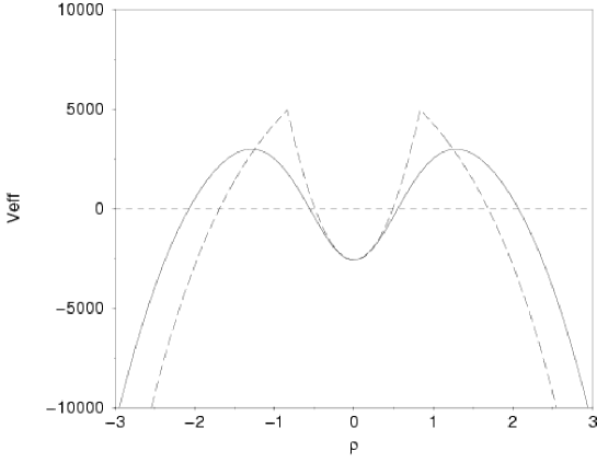
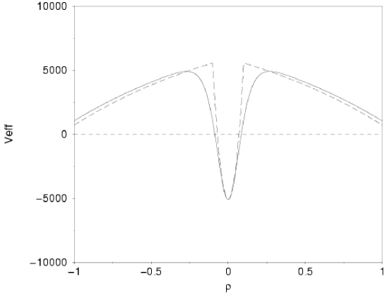
Figure 11.4: The effective potential $V_{{}_{\rm eff}}=-\omega^{2}$ and the approximate analytic effective potential (dashed curve) obtained from the matching of its two asymptotic expansions near the brane and at infinity. On the first panel, the parameters are the same as on Fig. 11.3, i.e. $\gamma_{{}_{\mathrm{F}}}=100$ and $\mu=0.5\gamma_{{}_{\mathrm{F}}}$. As the asymptotic solution is not reached very close to the brane, the approximation is rather poor and the two solutions are not in good agreement at intermediate regions. On the panel, we use the new parameter values $\gamma_{{}_{\mathrm{F}}}=100$ and $\mu=0.6\gamma_{{}_{\mathrm{F}}}$, obtained for $\alpha=0.1865$ and $\beta=53.62$, a much better approximation is obtained around the potential barrier provided the Higgs field and warp factor reach their vacuum value rapidely, i.e. for larger value of $\alpha\beta$. As on Fig. 11.3, the parameters are chosen to illustrate the point and do not necessarily correspond to existing bound states.

$\varrho>\varrho_{{}_{\rm m}}$:

we introduce the new variable

$$z\equiv\sqrt{6}\mu{\mathrm{e}}^{|\varrho|/\sqrt{6}},$$ (11.61)

in terms of which Eq. (11.59) reduces to a standard Bessel differential equation

$$\left[\frac{{\mathrm{d}}^{2}}{{\mathrm{d}}z^{2}}+\frac{1}{z}\frac{{\mathrm{d}}}{{\mathrm{d}}z}+\left(1-\frac{\ell^{2}}{z^{2}}\right)\right]\,\widehat{\mathcal{U}}_{\rm L}=0,$$ (11.62)

the order of which being given by

$$\ell=\sqrt{6}\gamma_{{}_{\mathrm{F}}}+\frac{1}{2}.$$ (11.63)

Since $\omega^{2}$ is positive at infinity, the asymptotic form of the solution is necessary radiative, as was already pointed out in the previous section. The most general solution of the Bessel equation (11.62) is a linear superposition of Hankel functions. Since we are interested only in ingoing waves in order to study a tunneling process, the most general solution takes the form

$$\widehat{\mathcal{U}}_{\rm L}(z)=B\,H^{(1)}_{\ell}(z),$$ (11.64)

where $H^{(1)}_{\ell}(z)$ is the Hankel function of the first kind, propagating towards the brane at infinity [2]

$$H^{(1)}_{\ell}(z\rightarrow\infty)\sim\sqrt{\frac{2}{\pi z}}\,{\mathrm{e}}^{i(z-\ell\pi/2-\pi/4)}.$$ (11.65)

and $B$ is an arbitrary complex constant.

$\varrho<\varrho_{{}_{\rm m}}$:

performing operations similar to those of the previous case, we cast Eq. (11.60) on the form

$$\left[\frac{{\mathrm{d}}^{2}}{{\mathrm{d}}x^{2}}-\left(\frac{1}{4}x^{2}+a\right)\right]\widehat{\mathcal{U}}_{\rm L}=0,$$ (11.66)

in which we have introduced the new variable and parameter

$$x\equiv\left(4\Omega\right)^{\frac{1}{4}}\varrho,\ \ \ \ \ a\equiv-\frac{\omega_{0}^{2}}{2\sqrt{\Omega}}.$$ (11.67)

The general solutions of Eq. (11.66) are the parabolic cylinder functions, namely $U(a,x)$ and $V(a,x)$, of which $\widehat{\mathcal{U}}_{\rm L}(x)$ can be expressed as linear superpositions. In the limit $x\gg|a|$, these solutions scale as [254]

$$U(a,x)\sim{\mathrm{e}}^{-\frac{1}{4}x^{2}}x^{-a-\frac{1}{2}}, V(a,x)\sim\sqrt{\frac{2}{\pi}}\,{\mathrm{e}}^{\frac{1}{4}x^{2}}x^{a-\frac{1}{2}}.$$ (11.68)

Since we are interested in confined fermion states on the brane, only the exponentially decreasing function is relevant, so that the general solution near the brane reads

$$\widehat{\mathcal{U}}_{\rm L}(x)=A\,U(a,x),$$ (11.69)

where $A$ is a complex integration constant.

The general solution $\widehat{\mathcal{U}}_{\rm L}(\varrho)$ for all $\varrho$ is obtained by matching the two different solutions at $\varrho=\varrho_{{}_{\rm m}}$. Since $\varrho_{{}_{\rm m}}$ corresponds to the maximum positive value of the effective potential [see Fig. 11.4], it is reasonable to consider that the Hankel function at that point can be expanded around small values of their argument with respect to their order [2], i.e.

$$H^{(1)}_{\ell}(z_{{}_{\rm m}})\sim-\frac{2^{\ell}}{\pi}\Gamma(\ell)z_{{}_{\rm m}}^{-\ell},$$ (11.70)

while the parabolic cylinder functions can be taken in their large argument asymptotic limit (11.68). This is the same kind of approximation as that made to derive the effective potential. Physically, the initial conditions on the brane, i.e. $\widehat{\mathcal{U}}_{\rm L}(0)$ and $\partial_{\varrho}\widehat{\mathcal{U}}_{\rm L}|_{0}$, are chosen in such a way that the asymptotic exponentially growing function $V(a,x)$ contribution is everywhere negligible. Once these initial conditions are fixed, they fully determine the solution on the other side of the brane, i.e. for $x<0$. The asymptotic expansion (11.68) can be analytically extended to $-|x|=|x|{\mathrm{e}}^{i\pi}$ and yields [163]

$$U(a,-|x|)\sim{\mathrm{e}}^{-\frac{1}{4}|x|^{2}}|x|^{-a-\frac{1}{2}}{\mathrm{e}}^{-i\pi\left(a+\frac{1}{2}\right)}.$$ (11.71)

Thus, once $\widehat{\mathcal{U}}_{\rm L}(0)$ and $\partial_{\varrho}\widehat{\mathcal{U}}_{\rm L}|_{0}$ are fixed, the matchings between $H^{(1)}_{\ell}(z_{{}_{\rm m}})$ and $U(a,-|x_{{}_{\rm m}}|)$ on one side, and $U(a,|x_{{}_{\rm m}}|)$ on the other side fully determine the bulk component $\widehat{\mathcal{U}}_{\rm L}$ for all $\varrho$.

The last constraint comes from Eq. (11.37) determining the right-handed spinor bulk function. It is well defined if and only if both $\widehat{\mathcal{U}}_{\rm L}$ and $\partial_{\varrho}\widehat{\mathcal{U}}_{\rm L}$ are not singular. In fact, the derivative of the parabolic cylinder function $U(a,x)$ is generally discontinuous at $x=0$. With the help of the Wronskian of $U(a,x)$ and $U(a,-x)$ [254]

$$U(a,x)\frac{{\mathrm{d}}U(a,-x)}{{\mathrm{d}}x}-U(a,-x)\frac{{\mathrm{d}}U(a,x)}{{\mathrm{d}}x}=\frac{2\pi}{\Gamma\left(\frac{1}{2}+a\right)},$$ (11.72)

we can construct the derivative discontinuity at $x=0$. This is

$$\frac{{\mathrm{d}}U(a,0^{-})}{{\mathrm{d}}x}-\frac{{\mathrm{d}}U(a,0^{+})}{{\mathrm{d}}x}=2^{\frac{a}{2}+\frac{3}{4}}\frac{\Gamma\left(\frac{3}{4}+\frac{a}{2}\right)}{\Gamma\left(\frac{1}{2}+a\right)},$$ (11.73)

where we have used the particular value [254]

$$U(a,0)=\frac{\sqrt{\pi}}{2^{\frac{a}{2}+\frac{1}{4}}\Gamma\left(\frac{3}{4}+\frac{a}{2}\right)}.$$ (11.74)

Imposing that the derivative of $\widehat{\mathcal{U}}_{\rm L}$ is continuous at $x=0$ results in imposing that the jump (11.73) vanishes. This is the case if and only if $a$ is solution of

$$\frac{\Gamma\left(\frac{3}{4}+\frac{a}{2}\right)}{\Gamma\left(\frac{1}{2}+a\right)}=0.$$ (11.75)

Since $\Gamma$ is singular for negative integer arguments, this condition is satisfied only for

$$-a-\frac{1}{2}=2n,$$ (11.76)

where $n$ is a positive integer. Note that $-a-1/2$ cannot be odd since then the numerator of the Wronskian (11.75) will also be singular resulting in a finite derivative jump at $x=0$. The condition (11.76) shows that the trapped fermions on the brane have necessarily discrete masses $\mu_{n}$ which read, using the values of the parameters (11.52), (11.53) and (11.67),

$$\mu^{2}_{n} = \gamma_{{}_{\mathrm{F}}}H_{1}\left[(4n+1)\sqrt{1+\frac{6\beta}{3\gamma_{{}_{\mathrm{F}}}H_{1}}+\frac{24\alpha\beta+\alpha^{2}H_{1}^{2}\left[(4n+1)^{2}-5\right]}{36\gamma_{{}_{\mathrm{F}}}^{2}}}\right.$$ (11.77)

$$-\left.\left(1+\frac{\alpha H_{1}}{6\gamma_{{}_{\mathrm{F}}}}\left[(4n+1)^{2}+1\right]\right)\right].$$

This mass spectrum is valid for $n>0$ since our derivation assumed that $\mu>0$. In the limiting case where $\gamma_{{}_{\mathrm{F}}}\gg 1$, it reduces to the much simpler form for the lowest masses

$$\mu_{n}\sim 2\sqrt{n}\sqrt{\gamma_{{}_{\mathrm{F}}}H_{1}}.$$ (11.78)

On the other hand, $\mu^{2}$ cannot reach very large values since it is necessary to have a potential barrier in order to have bound states. From the expression of the effective potential (11.54), the barrier is found to disappear when

$$\omega_{\infty}^{2}(\varrho_{{}_{\rm m}},\mu_{\max})\sim 0.$$ (11.79)

Again in the limit where $\gamma_{{}_{\mathrm{F}}}\gg 1$, using the value (11.58) of $\varrho_{{}_{\rm m}}$, one gets the maximum accessible reduced mass $\mu_{\max}$ for $\mu$ as

$$\mu_{\max}\sim\gamma_{{}_{\mathrm{F}}}{\mathrm{e}}^{-1/\sqrt{6}H_{1}}.$$ (11.80)

The maximum number of distinct massive states trapped on the brane can thus be estimated to be

$$n_{\max}\sim{\mathrm{Int}}\left[\gamma_{{}_{\mathrm{F}}}\frac{1}{4H_{1}}{\mathrm{e}}^{-2/\sqrt{6}H_{1}}\right].$$ (11.81)

For the parameters chosen in Fig. 11.3, one obtains $\mu_{\max}\sim 0.68\gamma_{{}_{\mathrm{F}}}$ and there are $n_{\max}=11$ massive modes trapped on the brane.

11.4.3 Fermion tunneling rate

Since the effective potential becomes negative at infinity, the massive modes trapped on the brane are subject only to a finite potential barrier. They are in a metastable state and can tunnel from the brane to the bulk. In this section we use our previous analytic solution to estimate the tunneling rate. Would this rate be too high, one would observe an effective violation of energy-momentum conservation on the brane, i.e. in four dimension, thereby contradicting observation.

Our starting point is the analytic solution for the left-handed bulk function that was derived in the previous section

$$\varrho<\varrho_{{}_{\rm m}} \Rightarrow \widehat{\mathcal{U}}_{\rm L}(\varrho)=A\,U\left(a,\sqrt{2}\Omega^{1/4}\varrho\right),$$ (11.82)

$$\varrho>\varrho_{{}_{\rm m}} \Rightarrow \widehat{\mathcal{U}}_{\rm L}(\varrho)=B\,H^{(1)}_{\ell}\left(\sqrt{6}\mu{\mathrm{e}}^{|\varrho|/\sqrt{6}}\right).$$ (11.83)

The transmission factor can easily be derived from the matching conditions of the left-handed bulk fermion component at $\varrho=\varrho_{{}_{\rm m}}$. First of all, $\widehat{\mathcal{U}}_{\rm L}$ has to be continuous. Using the expansions (11.68) and (11.70) and the value (11.76) of the parameter $a$, permits to find the relation

$$A\,{\mathrm{e}}^{-\frac{1}{2}\sqrt{\Omega}\varrho_{{}_{\rm m}}^{2}}\left(2\sqrt{\Omega}\right)^{n}\varrho_{{}_{\rm m}}^{2n}=-\frac{i}{\pi}B\,\Gamma(\ell)\left(\sqrt{\frac{3}{2}}\mu_{n}\right)^{-\ell}{\mathrm{e}}^{-\ell\varrho_{{}_{\rm m}}/\sqrt{6}}$$ (11.84)

between the coefficients $A$ and $B$. Making use of the expression (11.58) for $\varrho_{{}_{\rm m}}$ yields

$$\frac{B}{A}=\frac{i\pi}{\Gamma(\ell)}\left(\sqrt{\frac{3}{2}}\mu_{n}\right)^{\ell}\left(\frac{\ell^{2}}{3\sqrt{\Omega}}\right)^{n}\exp{\left(\frac{\ell^{2}}{12\sqrt{\Omega}}\right)}.$$ (11.85)

Assuming, as above, that $\gamma_{{}_{\mathrm{F}}}\gg 1$ (so that $\ell\gg 1$) we can expand $\Gamma(\ell)$ as

$$\Gamma(\ell)\sim\ell^{\ell-1/2}{\mathrm{e}}^{-\ell}\sqrt{2\pi},$$ (11.86)

so that, using expressions (11.57), (11.58) and (11.63) respectively of $\Omega$, $\varrho_{{}_{\rm m}}$, and $\ell$, we get that $B/A$ is approximated by

$$\frac{B}{A}\sim i\sqrt{\frac{\pi}{2}}\left(\frac{2}{H_{1}}\right)^{n}6^{1/4}\gamma_{{}_{\mathrm{F}}}^{n+1/2}\exp{\left[-\sqrt{6}\gamma_{{}_{\mathrm{F}}}\left(\ln{\frac{2\mu_{\max}}{\mu}}-1+\frac{1}{2\sqrt{6}H_{1}}\right)\right]}.$$ (11.87)

The transmission coefficient from the brane to the bulk associated with $\widehat{\mathcal{U}}_{\rm L}$ can thus be defined by

$$\widehat{\mathcal{T}}\equiv\frac{\widehat{\mathcal{U}}_{\rm L}(\ell)}{\widehat{\mathcal{U}}_{\rm L}(0)},$$ (11.88)

with $\widehat{\mathcal{U}}_{\rm L}(\ell)=BH_{\ell}^{(1)}(\ell)$, is evaluated at the turning point $\varrho=\ell$ where the spinor bulk component begins to propagate freely. Using the behaviour (11.74) of the function at the origin, the ratio (11.87) and the properties [2] of the Hankel function

$$H^{(1)}_{\ell}(\ell)=\left(\frac{4}{3}\right)^{2/3}\frac{{\mathrm{e}}^{-i\pi/3}}{\Gamma(2/3)}\,\ell^{-1/3},$$ (11.89)

the transmission coefficient (11.88) reduces to

$$\widehat{\mathcal{T}}\sim\frac{2^{4/3}\Gamma(1/2-n)}{3^{7/12}\Gamma(2/3)}{\mathrm{e}}^{i\pi/6}H_{1}^{-n}\gamma_{{}_{\mathrm{F}}}^{n+1/6}\exp{\left[-\sqrt{6}\gamma_{{}_{\mathrm{F}}}\left(\ln{\frac{2\mu_{\max}}{\mu}}-1+\frac{1}{2\sqrt{6}H_{1}}\right)\right]}.$$ (11.90)

It follows, using the definition (11.40), that the probability for a trapped particle on the brane to tunnel to the bulk is given by

$${\mathcal{P}}\equiv|\widetilde{\mathcal{T}}|^{2}={\mathrm{e}}^{2\ell/\sqrt{6}}\,|\widehat{\mathcal{T}}|^{2}.$$ (11.91)

The characteristic time for a fermionic mode trapped on the brane can be roughly estimated by

$$\tau_{{}_{\mathrm{b}}}\sim y_{{}_{\rm b}}=\frac{\varrho_{{}_{\rm b}}}{\sqrt{|\Lambda|}},$$ (11.92)

where $y_{{}_{\rm b}}$ represents the typical length, in the fifth dimension, felt by a particle on the brane. As can be seen on Fig. 11.5, the spinor bulk components are exponentially damped as soon as the effective potential becomes positive. Thus $\varrho_{{}_{\rm b}}$ can be estimated by the solution of $\omega_{{}_{\rm b}}^{2}(\varrho_{{}_{\rm b}})=0$ so that, keeping in mind that $\mu<\gamma_{{}_{\mathrm{F}}}$,

$${\varrho_{{}_{\rm b}}}^{-1}\sim\sqrt{H_{1}\gamma_{{}_{\mathrm{F}}}}.$$ (11.93)

The life-time $\tau_{n}$ of a fermionic bound state on the brane labelled by $n$

$$\tau_{n}=\frac{\tau_{{}_{\rm b}}}{{\mathcal{P}}}$$ (11.94)

can be estimated by

$$\tau_{n} \sim \frac{3^{7/6}\,\Gamma^{2}(2/3)}{2^{11/6}\,\Gamma^{2}(1/2-n)}H_{1}^{2n-1/2}\frac{\gamma_{{}_{\mathrm{F}}}^{-2n-5/6}}{\sqrt{|\Lambda|}}\,$$ (11.95)

$$\times\exp{\left[2\sqrt{6}\gamma_{{}_{\mathrm{F}}}\left(\ln{\frac{2\mu_{\max}}{\mu_{n}}}-1-{1\over\sqrt{6}}+\frac{1}{2\sqrt{6}H_{1}}\right)\right]}.$$

We recall that, due to the approximations performed in the previous derivation, this estimate is valid only for $\mu\ll\mu_{\max}$. Nevertheless, the argument in the exponential amplifies the transition from bound states to tunneling ones for masses $\mu\sim\mu_{\max}$, as intuitively expected. An order of magnitude of the minimal coupling constant $\gamma_{{}_{\mathrm{F}}}$ leading to stable bound states can thus be estimated by requiring that the lowest massive state does not tunnel,

$$\mu_{1}<2\mu_{\max}\exp{\left(-1-{1\over\sqrt{6}}+\frac{1}{2\sqrt{6}H_{1}}\right)}.$$ (11.96)

Using the two values (11.78) and (11.80), this implies that

$$\gamma_{{}_{\mathrm{F}}}\gtrsim H_{1}\exp{\left(2+{2\over\sqrt{6}}+\frac{1}{\sqrt{6}H_{1}}\right)}.$$ (11.97)

As a numerical application, for the Higgs and gravity parameters used in Fig. 11.3, we get $\gamma_{{}_{\mathrm{F}}}\gtrsim 25$.

11.5 Numerical investigation

Numerically, it is simpler and more convenient to solve the first order differential system (11.30-11.31). A Runge-Kutta integration method was used, on both sides of the brane. In order to suppress the exponential growth, we integrate from the turning point, $\varrho=\ell$, where the solution begins to propagate freely, toward the brane. In this way, we get only $U(a,x)$ near the brane. The radiative solution for $\varrho>\ell$, is simply obtained by integrating from the turning point toward infinity, with initial conditions determined by the matching with the exponential decreasing solution near the wall. The same method is used on the other side of the brane, but this time, by means of the last free parameter, we impose the continuity of one bulk spinor component on the brane ($\widetilde{\mathcal{U}}_{\rm L}$ say). Generally, the other bulk spinor component will be discontinuous at $\varrho=0$, as expected from the analytical study since $U^{\prime}(a,0)$ is generally discontinuous. The mass spectrum is thus obtained by requiring the continuity of $\widetilde{\mathcal{U}}_{\rm R}$ on the brane.

The bulk spinor components computed this scheme have been plotted for the first massive modes trapped on the brane in Fig. 11.6, for $\gamma_{{}_{\mathrm{F}}}=100$. The lowest mass is numerically found to be $\mu_{1}\sim 0.209\gamma_{{}_{\mathrm{F}}}$ and was estimated analytically, from (11.78), to be $\mu_{1}\sim 0.210\gamma_{{}_{\mathrm{F}}}$ leading to a precision of 0.5% for the analytical estimate. The second mass is numerically found to be $\mu_{2}\sim 0.291\gamma_{{}_{\mathrm{F}}}$, which has to be compared to its analytical estimate $\mu_{2}\sim 0.295\gamma_{{}_{\mathrm{F}}}$. Again, the precision of this estimate is of about 1%. As predicted from (11.81), there are $n_{\max}=11$ massive bound states the lightest masses of which are summed up in table 11.1. On Fig. 11.5, we plot the last $n=11$ trapped mode; it has a tiny radiative component, as expected for a tunneling mode.

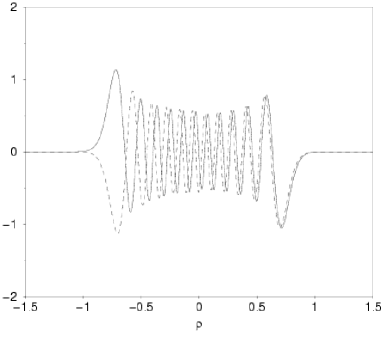
Figure 11.5: [Left] The right (dashed line) and left (solid line) bulk spinor components $\widetilde{\mathcal{U}}_{\rm R}$ and $\widetilde{\mathcal{U}}_{\rm L}$, as functions of the dimensionless distance $\varrho$ to the brane, for the heaviest massive state ($n=11$) and $\gamma_{{}_{\mathrm{F}}}=100$. [Right] Zoom near the turning point and transition to the radiative behaviour which takes place at a finite distance to the brane due to the tunneling of this mode from the brane to the bulk.

$n$	1	2	3	4	5	6	…	11
$\mu_{n}$ (numerical)	0.209	0.291	0.353	0.402	0.444	0.480	…	0.593
$\mu_{n}$ (estimates)	0.210	0.295	0.359	0.412	0.458	0.499	…	0.657
precision (%)	0.5	1.3	1.7	2.4	3	3.8	…	9.7

Table 11.1: Comparison of the numerical values and analytical estimates of the first six bound states reduced mass $\mu$, together with the heaviest mode, computed for $\gamma_{{}_{\mathrm{F}}}=100$.

In conclusion, the numerics confirm that the approximations of the previous section and our estimates are accurate up to 1%-10% (see table 11.1).

Figure 11.6: The right (dashed curve) and left bulk spinor components, $\widetilde{\mathcal{U}}_{\rm R}$ and $\widetilde{\mathcal{U}}_{\rm L}$, as functions of the dimensionless distance $\varrho$ from the brane for the lightest massive bound states. They have been computed for $\gamma_{{}_{\mathrm{F}}}=100$ and in the Higgs and warp factor profiles obtained with parameter of Fig. 11.3. The numerical values of the corresponding reduced masses are reported on table 11.1.

11.6 Discussion and conclusions

We shall now discuss the cosmological constraints existing on the kind of model we have been considering here. Most of these constraints come from brane models in which the wall structure is replaced by an infinitely thin four dimensional layer. As discussed in the previous sections, such an approximation is equivalent, within our framework, to asking that the combination $\alpha\beta$ be much larger than unity. In this limit, equivalent to the large $\beta$ limit since, from Eq. (11.15), $\alpha\beta\sim{4\over 3}\beta^{1/2}$, we can replace the stress-energy tensor (11.6) by the effective four dimensional surface distribution

$$T^{{}^{\rm eff}}_{\mu\nu}=T_{\infty}g_{\mu\nu}\delta(y),$$ (11.98)

whose isotropic tension $T_{\infty}$ is obtained by integration in the transverse direction to yield

$$T_{\infty}=\sqrt{|\Lambda|}\eta^{2}\int{\mathrm{d}}\varrho\,{\mathrm{e}}^{-6\sigma(\varrho)}\left[{1\over 2}\Phi^{\prime 2}+2V\right]\equiv\sqrt{|\Lambda|}\eta^{2}\xi(\beta)$$ (11.99)

where the function $\xi(\beta)$ can be expressed as

$$\xi=\int{\mathrm{d}}\varrho\,{\mathrm{e}}^{-6\sigma(\varrho)}\left[{6S^{2}-1\over\alpha}+2\beta(H^{2}-1)^{2}\right].$$ (11.100)

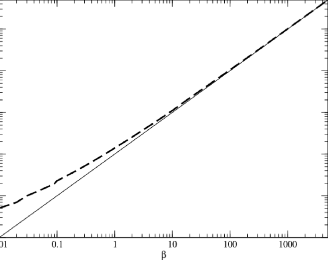
Figure 11.7: Effective four dimensional brane tension, in units of $\sqrt{|\Lambda|}\eta^{2}$, of the domain wall as a function of $\beta$ (dashed line). It is clear that in the thin brane limit, $\xi\simeq\beta$ (thin line).

Fig. 11.7 shows the variation of $\xi$ as a function of $\beta$. In the limit $\beta\gg 1$, it is clear that $\xi\simeq\beta$, so that the brane tension behaves as

$$T_{\infty}\simeq{\lambda\eta^{4}\over 8\sqrt{|\Lambda|}},$$ (11.101)

which will be used to derive the relevant cosmological constraints. Note also that the discrepancy between the above formula and the actual value of $T_{\infty}$ becomes important (more than 100 % error say) for $\beta\lesssim 0.1$, which is already rather far from the thin brane limit usually considered.

11.6.1 Investigation of the parameter space

The model described in this article depends of five parameters, four describing the spacetime and scalar field dynamics $({\mathcal{G}}_{{}_{5}},\Lambda,\eta,\lambda)$ and one concerning the fermions $(g_{{}_{\rm F}}$). With the domain wall structure assumed, only four of these parameters are independent [see Eq. (11.16)]. It is convenient to replace this set of parameters by the three mass scales

$$m_{{}_{5}}\equiv{\mathcal{G}}_{{}_{5}}^{-1/3},\qquad m_{{}_{\Lambda}}\equiv\frac{\sqrt{-\Lambda}}{6},\qquad m_{{}_{\infty}}\equiv T_{{}_{\infty}}^{1/4},$$ (11.102)

and the dimensionless parameter $\gamma_{{}_{\rm F}}$. These parameters are subject to a number of constraints, namely:

The four dimensional gravitational constant must agree with its observed value $G_{{}_{4}}\equiv m_{{}_{4}}^{-2}$ with $m_{{}_{4}}\sim 10^{19}\,$GeV. Using the expression of the four dimensional Planck mass in terms of the five dimensional analog and of the brane tension gives [39, 100, 90, 38, 219, 315, 140, 241, 306, 77, 28]

$$m_{{}_{5}}^{3}\sim m_{{}_{4}}m_{{}_{\infty}}^{2}.$$ (11.103)

The brane cosmological constant [39, 100, 90, 38, 219, 315, 140, 241, 306, 77, 28]

$$2\Lambda_{{}_{4}}=\Lambda+6\pi^{4}{\mathcal{G}}_{{}_{5}}^{2}T_{{}_{\infty}}^{2},$$ (11.104)

must also agree with the standard observational bound $m_{\Lambda_{4}}<10^{-60}m_{{}_{4}}$. This implies

$$m_{{}_{\Lambda}}=\frac{\pi^{2}}{\sqrt{6}}\frac{m_{{}_{\infty}}^{4}}{m_{{}_{5}}^{3}} \Rightarrow m_{\infty}^{4}\sim m_{\Lambda}m_{5}^{3}.$$ (11.105)

Note that in the limit $\beta\gg 1$, this relation is equivalent to Eq. (11.101). This means that this condition is readily satisfied in the thin brane limit. At this point, it is worth emphasizing that this is precisely the limit in which the analytic approximation for fermion masses are the most accurate.

There must not be any deviation of the law of gravity on the brane with respect to the inverse square Newton law above 1 millimeter [238]. This implies [88]

$$m_{{}_{\Lambda}}\gtrsim 10^{-3}\,\mathrm{eV}.$$ (11.106)

Finally, we require the fermion stress-energy tensor to be negligible with the brane stress-energy, so that we impose that the mass of the heaviest fermion is smaller than the brane mass scale. By means of Eq. (11.80), this condition reads

$$m_{\max}\sim m_{\Lambda}\gamma_{{}_{\mathrm{F}}}{\mathrm{e}}^{-1/(\sqrt{6}H_{1})}<m_{\infty},$$ (11.107)

where $H_{1}$ ends up being function of $\beta$ only by means of Eqs (11.15) and (11.50),

$$H_{1}^{2}=2\beta-\frac{6\beta}{\sqrt{16\beta+9}}.$$ (11.108)

In the limit $\beta\gg 1$, Eqs. (11.107) and (11.108) combine to give the constraint on the coupling constant

$$\gamma_{{}_{\mathrm{F}}}<{m_{\infty}\over m_{\Lambda}}{\mathrm{e}}^{1/\sqrt{12\beta}}\simeq{m_{\infty}\over m_{\Lambda}}.$$ (11.109)

It follows from the relations (11.103) and (11.105) that $m_{\infty}^{2}\sim m_{\Lambda}m_{4}$ so that the three mass scales must satisfy

$$m_{{}_{\Lambda}}\gtrsim 10^{-3}\,{\rm eV},\qquad m_{{}_{\infty}}\gtrsim 1\,{\rm TeV},\qquad m_{{}_{5}}\gtrsim 10^{6}\,{\rm TeV},$$ (11.110)

which, together with Eq. (11.109) and (11.35) yields

$${1\over 2\sqrt{6}}<\gamma_{{}_{\mathrm{F}}}\lesssim 10^{15}\left({m_{\infty}\over 1\,\hbox{TeV}}\right),$$ (11.111)

where, as discussed below Eq. (11.40), the lower bound is very conservative.

Now, let us examine the stability of the fermion confinement on the brane and the restriction on their life-time imposed by the previous conditions. We require, at least, one massive bound state to have a life-time longer than the age of the Universe, i.e.

$$\tau_{1}>\tau_{\mathrm{univ}}\sim 10^{17}\mathrm{s}.$$ (11.112)

Using Eq. (11.95), one roughly gets

$$m_{\Lambda}\tau_{1}\sim\Upsilon(\beta,\gamma_{{}_{\mathrm{F}}})\equiv H_{1}^{3/2}\gamma_{{}_{\mathrm{F}}}^{-17/6}\exp{\left[2\sqrt{6}\gamma_{{}_{\mathrm{F}}}\left(\frac{1}{2}\ln{\frac{\gamma_{{}_{\mathrm{F}}}}{H_{1}}}-1-1/\sqrt{6}-\frac{1}{2\sqrt{6}H_{1}}\right)\right]}.$$ (11.113)

The condition (11.112) together with the former constraint (11.110) can be written as

$$\Upsilon(\beta,\gamma_{{}_{\mathrm{F}}})\gtrsim 10^{30}.$$ (11.114)

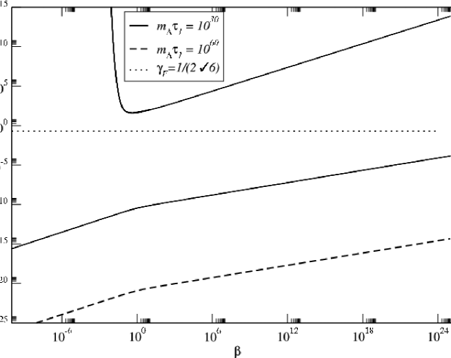
Figure 11.8: Contour plot of the function $\Upsilon(\beta,\gamma_{{}_{\mathrm{F}}})$ for $\Upsilon=10^{30}$ [solid lines] and $10^{60}$ [dashed line], i.e. respectively a particle life-time of the order of the age of the Universe, and of the proton life-time lower limit. Note that both top curves are indistinguishable due to the exponential behavior of $\Upsilon$ in $\gamma_{{}_{\mathrm{F}}}$. They turn out to be equivalent to the analytical requirement given by Eq. (11.97). Points above the highest curve and below the lowest curves satisfy the contraint. We also superimpose the conservative constraint (11.35) necessary for the existence of a massless bound state, the allowed region being above the dotted line.

On Fig. 11.8, we present the contour plot of the dimensionless function $\Upsilon(\beta,\gamma_{{}_{\mathrm{F}}})$, for $\Upsilon=10^{30}$ and $10^{60}$, which correspond respectively to a particle life-time of the order of the age of the Universe, and of the proton life-time lower limit. For $\beta\gtrsim 1$, there are in principle two allowed regions, corresponding to strong and weak coupling limits, i.e. $\gamma_{{}_{\mathrm{F}}}\gg 1$ and $\gamma_{{}_{\mathrm{F}}}\ll 1$. However, the lower bound on $\gamma_{{}_{\mathrm{F}}}$, which comes from the requirement that fermions are actually trapped on the brane, pushes the weak coupling allowed region to very high values of $\beta$, in practice $\beta\gtrsim 7.5\times 10^{57}$ for $\Upsilon=10^{30}$. Note also that this already rather extreme value is based on the conservative estimate given by Eq. (11.35).

For $\beta\lesssim 1$, the weak coupling region completely disappears, while the strong coupling allowed region shrinks rapidely: for $\beta\lesssim 8.5\times 10^{-3}$, the life-time cannot exceed the age of the Universe because $\gamma_{{}_{\mathrm{F}}}\gtrsim 10^{15}$. Considering $\beta\gtrsim 1$ therefore turns out to be the relevant limit if one wishes to have fermionic bound states living on the brane.

11.6.2 Conclusion

In this article, we have considered fermions coupled to a Higgs field with a domain wall structure in a five dimensional anti-de Sitter spacetime. This domain wall can be thought of as a realization of a brane universe.

After, studying the domain wall configuration, we solved the Dirac equation and showed that there exists massive fermionic bound states trapped on the wall. We develop both analytic approximation to compute the mass spectrum and the tunneling time. This was compared to a full numerical integration of the dynamical equations that revealed the accuracy of our approximation scheme.

We recover the fact that massive fermions tunnel to the bulk [121]. Investigation in the parameter space shows that, for models satisfying the cosmological constraints, the relevant confinement life-time can be much greater that either the age of the Universe or the proton life-time. This was made possible by the derivation of the analytic estimate.

One of our central result is the derivation of an analytic mass spectrum for fermions trapped on a brane-like four dimensional spacetime. In particular, as could have been anticipated [262], it was shown that the allowed masses are quantized, with a spectrum varrying, in the strong coupling limit, as $\sqrt{n}$. Such a spectrum is indeed in contradiction with experimental measurements of particle masses [164], which is not surprising given the simplicity of the model. It however opens the possibility to build more realistic theories in which mass quantization would stem naturally from extra dimensions.

Acknowledgments

We thank Jérôme Martin for numerous enlightening discussion, and in particular for pointing to us Ref. [254] on parabolic cylinder functions. JPU thanks l’Institut d’Astrophysique de Paris for hospitality while this work was carried out.

Conclusion

Les principaux résultats de cette thèse concernent le confinement de fermions sur des objets étendus de type cordes cosmiques et branes en dimensions supplémentaires.

Du point de vue de la physique des particules, il y est montré qu’un couplage de Yukawa entre des champs fermioniques et un champ de Higgs inhomogène, de type défaut topologique, conduisait, de manière générique, à l’existence d’états liés dont le spectre de masse a été étudié en détail. La prise en compte de l’effet des courants générés par le remplissage de ces états sur le spectre lui-même semble montrer que l’état fondamental ne peut pas être de masse nulle, invalidant de ce fait l’existence physique de modes zéros dans ces modèles. Ce résultat remet en cause les études précédentes sur les courants de fermions dans les cordes, tant du point de vue microscopique que cosmologique.

D’un point de vue cosmologique, ces résultats nous ont permis, dans un premier temps, d’étudier la dynamique des cordes cosmiques parcourues par des courants de fermions, et d’en extraire une équation d’état. Contrairement aux cas connus des cordes possédant des courants de bosons, cette équation d’état met en jeu plusieurs paramètres internes qui s’identifient aux densités des divers fermions présents dans la corde. Ce résultat fait qu’il n’est pas toujours possible d’appliquer le formalisme covariant à un paramètre pour les courants de fermions. Ces courants se distinguent également de ceux de bosons, dans la dynamique des cordes, par le fait qu’ils privilégient à la fois des régimes subsoniques, lorsque les courants sont ultrarelativistes, et des régimes supersoniques, lorsque les modes massifs sont prédominants. Les vortons associés à ces deux types de dynamique sont alors classiquement respectivement stables et instables. Leur persistance au cours de l’évolution de l’univers pouvant conduire à une catastrophe cosmologique, les conséquences des transitions entre les régimes de stabilité et d’instabilité de ces vortons pourraient être importantes.

En ce qui concerne la cosmologie en dimensions supplémentaires, le mécanisme de confinement étudié sur les cordes a permis de proposer une solution simple au problème de la localisation des fermions massifs sur une brane représentant notre univers. Il est ainsi possible de donner une explication à la quantification de la masse, en général, par l’existence d’un spectre de masse naturellement discret des états liés fermioniques. La prise en compte des effets gravitationnels a cependant montré que ces modes pouvaient s’échapper dans la dimension supplémentaire, et, en imposant que la durée de vie de ces états soit plus grande que l’âge de l’univers, des contraintes numériques sur les paramètres du modèle ont pu être trouvées.

Le prolongement naturel de ces travaux porte à la fois sur l’aspect cosmologique et microscopique. Concernant le premier, la réalisation de simulations numériques d’évolution de cordes conductrices permettrait de fixer précisément les contraintes cosmologiques qu’elles doivent vérifier, et, par le biais de l’équation d’état, de contraindre la physique des particules sous-jacente. Par analogie avec des cordes sans structure interne, l’évolution de ces réseaux doit être étroitement liée à la formation et à la persistance des vortons qu’ils produisent. Bien que classiquement stables pour les régimes subsoniques, des effets quantiques pourraient toutefois les déstabiliser. Il serait donc intéressant de pouvoir généraliser l’approche introduite dans cette thèse aux cas de cordes courbées, et d’en étudier les conséquences sur les états liés fermioniques.

En prolongement de l’étude du confinement des fermions massifs sur un mur de domaine quadri-dimensionnel, leur localisation sur une corde quadri-dimensionnelle plongée dans un espace-temps à six dimensions permettrait d’introduire leur charge. En effet, la corde étant générée par la brisure d’une symétrie locale, elle met en jeu un champ de jauge auquel les fermions sont couplés. Le spectre de masse des fermions chargés pourrait ainsi être comparé aux observations afin d’étudier la viabilité de ces modèles. De plus, comme pour les cordes, l’influence de la courbure de la brane sur le spectre de masse reste à étudier.

Annexes

Parallélisation numérique

11.7 Introduction

Dans le chapitre 5, nous avons présenté des résultats issus de simulations numériques faisant évoluer un réseau de cordes cosmiques de Goto-Nambu dans un univers de FLRW, à partir de diverses configurations initiales. La physique régissant l’évolution d’un tel réseau ayant été décrite dans les chapitres 4 et 5, cette annexe est consacrée aux aspects purement numériques du calcul. La résolution des équations du mouvements (5.18), ainsi que la détection et la réalisation des intercommutations entre les cordes, sont les deux tâches essentielles qui guident le calcul numérique. Cependant, celles-ci doivent être en permanence accompagnées de multiples vérifications et corrections afin d’éviter la croissance d’erreurs purement numériques, dues à la précision finie des machines. Dans le code utilisé ici, ce travail a été effectué par F. Bouchet et D. Bennett dans les années 1980 [33, 31], à l’aide du langage de programmation Fortran77. Cependant, l’utilisation actuelle de ce code, pour le calcul du spectre de fluctuation du CMBR induit par les cordes, requiert une grande dynamique temporelle de simulation. Or, la taille finie du volume dans lequel le réseau évolue fixe également la durée de la simulation, l’horizon devant y être toujours confiné pour éviter des effets de bord parasites (voir Chap. 5). Typiquement, les volumes, et donc les durées de simulation maximales de l’époque, étaient de l’ordre de $(26\ell_{\mathrm{c}})^{3}$, permettant d’étudier l’évolution cosmologique du réseau pour un accroissement du facteur d’échelle d’un facteur quinze dans l’ère de matière, contre un facteur six dans l’ère de radiation. Le nombre initial de points, par unité de longueur, utilisé pour décrire chaque corde est également un paramètre significatif. Il fixe la taille physique admissible des plus petites boucles qui ne peuvent être représentées que par trois points minimum. Ce cutoff est également exprimé en fonction de la longueur de corrélation de la transition de phase $\ell_{\mathrm{c}}$ (voir Chap. 5), et sa valeur typique est d’environ $0.3\ell_{\mathrm{c}}$, soit un nombre initial de points par longueur de corrélation de $10/\ell_{\mathrm{c}}$. Si l’on souhaite augmenter la résolution des simulations sur la taille des petites boucles, ce paramètre est également à augmenter.

Hormis l’accroissement des performances des machines actuelles, la mise en place de simulations numériques de hautes résolutions peut être opérée par le biais de méthodes de parallélisation. Celles-ci consistent essentiellement à reprogrammer le code afin que ses calculs, initialement opérés successivement, soient partagés entre différents processeurs, ou machines, dans le but d’augmenter la vitesse effective d’exécution. Il n’est cependant pas possible de paralléliser tout un code, certaines parties nécessitant toujours une exécution séquentielle. Les sections suivantes illustrent les améliorations effectuées, ainsi que les difficultés rencontrées, lorsque ces méthodes ont été développées sur le code de F. Bouchet, et dont les résultats provisoires ont été présentés dans le chapitre 5.

11.8 Directives de compilation OpenMP

Le langage qui a été utilisé pour paralléliser le code correspond au standard OpenMP apparu en 1997 [296], et remis à jour en novembre 2000 [296]. Bien que la parallélisation multitâches existe depuis quelques années, chaque constructeur possède son propre jeu de directives, et le standard OpenMP est actuellement le seul langage unifié et répandu. Sa jeunesse est cependant également responsable de son instabilité, et son fonctionnement correct à requis certaines reprogrammations du code à l’aide du langage Fortran90.

11.8.1 Parallélisation des autocommutations

L’identification des parties du programme pouvant être parallélisées est souvent directement donnée par la physique qu’elles modélisent. Le critère déterminant est que les sections parallèles doivent être indépendantes, c’est-à-dire que le résultat donné par une section parallèle doit être indépendant du résultat donné par l’autre section. Lorsque ce n’est pas le cas, la structure et l’exécution séquentielle du programme doivent être préservées pour conserver la validité des résultats.

Dans le code d’évolution de cordes cosmiques, l’étape demandant le plus de temps de calcul est la détection et la réalisation des autocommutations. Comme on peut le voir sur la figure 11.9, le sous programme nommé “iniselfc” occupe près de $80\%$ du temps d’exécution. Sa fonction dans le code est d’initialiser des variables relatives aux autocommutations de chaque boucle de corde en construisant une liste de points, sur la boucle en question, susceptibles de se croiser. Il est appelé pour chaque point de chaque boucle de corde et ne concerne que les points de la dite boucle. Il est clair qu’une telle opération peut être exécutée en parallèle car la détection d’un croisement est propre à chaque boucle. En fait, dans le but d’augmenter au maximum “l’épaisseur” des sections parallèles, ceci suggère de séparer le calcul de l’évolution de chaque corde sur les différents processeurs accessibles. Cette opération est cependant limitée par le fait qu’il existe des intercommutations entre les différentes cordes. Dans ce cas, il faut revenir à une exécution en série.

Figure 11.9: Temps de calcul passé dans les plus lents sous programmes du code d’évolution de cordes cosmiques lorsqu’il est exécuté en série. La détection des autocommutation occupe près de $80\%$ du temps total.

La séparation des tâches entre les divers processeurs peut simplement être mise en place à l’aide de directives de compilation, i.e. de commandes insérées dans le code donnant les instructions nécessaires au compilateur. Dans le langage OpenMP, la parallélisation sur chaque corde s’est effectuée par la directive !$OMP PARALLEL DO appliquée à une boucle de calcul DO séparant le traitement des différentes cordes (voir Fig. 11.10).

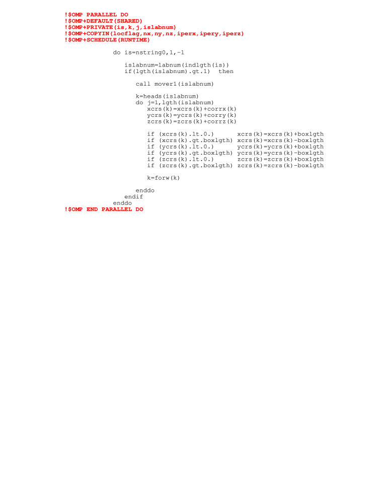
Figure 11.10: Directive de compilation !$OMP PARALLEL DO permettant l’exécution en parallèle de la boucle de calcul, selon son indice, ici is. L’ensemble des jeux d’instruction intérieurs à la boucle de calcul DO est exécuté par un processeur différent pour chaque valeur de is, modulo le nombre total de processeurs.

L’effet de cette directive est de faire calculer chaque bloc de commandes, situé entre !$OMP PARALLEL DO et !$OMP END PARALLEL DO, par chaque processeur accessible, le numéro du processeur étant relié à l’indice is, modulo le nombre total de processeurs. Il est de plus possible d’améliorer la dynamique de répartition des tâches par une directive nommée !$OMP SCHEDULE (voir Fig. 11.10). Celle-ci spécifie dans quel ordre les blocs de calcul indexés par is sont répartis sur les processeurs. Le choix le plus efficace est obtenu par l’option DYNAMIC qui affecte une tâche is quelconque au premier processeur libre ayant terminé le calcul d’un bloc antérieur. On évite de cette manière que des blocs de calcul plus long que les autres ne ralentissent l’exécution en parallèle.

Les autres directives de compilation apparaissant dans tout le reste du code (voir Fig. 11.11) gèrent le partage de la mémoire entre les différentes régions parallèles.

Figure 11.11: Le code d’évolution de cordes cosmiques de F. Bouchet et D. Bennett [33, 31]. Environ deux cents directives de compilation OpenMP ont été introduites pour sa parallélisation et sont représentées en rouge.

11.8.2 Les variables partagées

La principale difficulté lorsqu’une partie du code est parallélisée est de définir exactement quelles sont les variables qui vont être communes, ou non, à chaque section parallèle, i.e. à chaque corde dans le cas qui nous concerne. Par exemple, la plus évidente des variables privées est l’indice is: sa valeur est nécessairement différente pour chaque corde, par contre, le nombre total de cordes nstring0 est une variable partagée (voir Fig. 11.10). Les spécifications de partage des variables sont exécutées par les clauses SHARED ou PRIVATE sur la figure 11.10, pour déclarer des variables communes ou privées, respectivement.

Dans le code utilisé ici, près de deux cents directives de ce type ont été introduites afin de correctement déclarer le type de chaque variable (voir fig. 11.11). La deuxième difficulté apparaît lorsqu’une section parallèle modifie une variable partagée entre tous les processeurs. C’est par exemple le cas de nstring0: lors des autocommutations de chaque corde, de nombreuses petites boucles sont formées (voir Chap. 5) et dans toutes les sections parallèles il y a une instruction du type

$$\mathtt{nstring0}=\mathtt{nstring0}+1.$$ (11.115)

Pour que la valeur finale soit correcte, il ne faut absolument pas que deux processeurs accèdent en même temps à nstring0. Ceci peut être spécifié par les commandes !$OMP CRITICAL et !$OMP END CRITICAL qui assurent que le bloc d’instruction compris entre ces deux directives n’est jamais effectué simultanément par deux sections parallèles. L’écriture correcte de l’instruction (11.115) devient finalement

$$\begin{array}[]{lll}\mathtt{!{\$}OMP\ CRITICAL}&&\\ &\mathtt{nstring0}=\mathtt{nstring0}+1&\\ \mathtt{!{\$}OMP\ END\ CRITICAL}&&\end{array}$$ (11.116)

Enfin, une fois les variables correctement déclarées et calculées dans les sections parallèles, il faut s’assurer qu’elles sont correctement reliées à leur analogue dans les parties en série du programme, et inversement. Pour cela, on utilise la clause !$OMP COPYIN. Sur la figure 11.10, elle permet de copier la valeur des variables utilisées dans la section en série vers les variables privées des sections parallèles.

Le test suffisant, mais non nécessaire, permettant de vérifier si ces diverses étapes de parallélisation ont été correctement programmées, est ensuite de comparer les résultats entre le programme initial et le programme parallélisé. Les valeurs des diverses quantités physiques ont ainsi été retrouvées, à la précision de la machine près, entre les deux types d’exécution. Sur la figure 11.12, sont représentés les courbes de vitesse d’exécution instantanée du programme parallélisé lorsqu’il fonctionne sur deux, quatre, six ou huit processeurs. On voit clairement que l’augmentation du nombre de processeurs est de moins en moins efficace: le gain de temps entre six et huit processeurs est relativement minime. Cette limite dépend de plusieurs critères qui seront évoqués dans la section suivante.

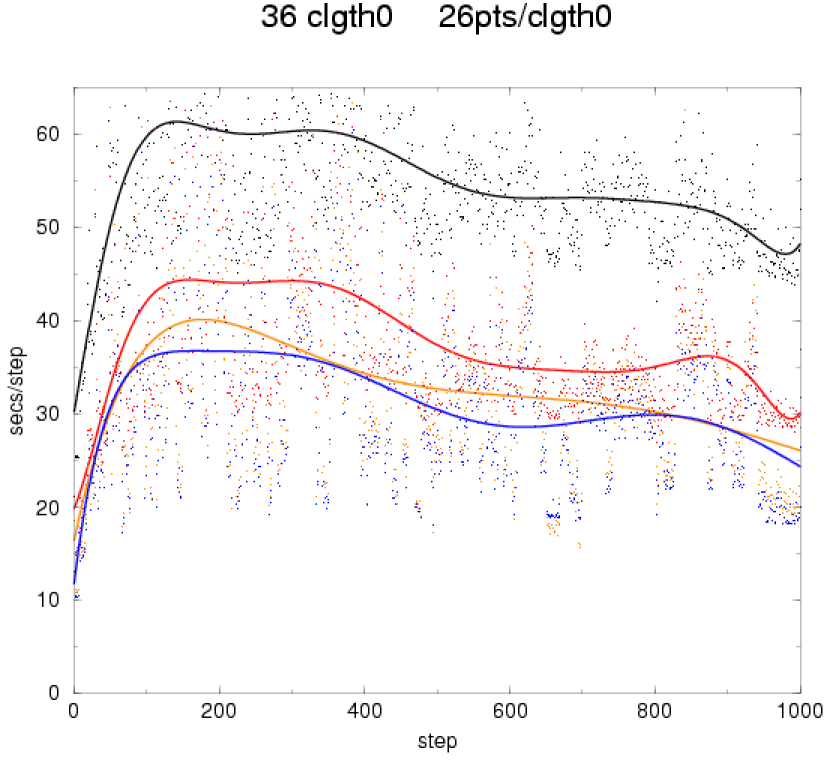
Figure 11.12: Temps d’exécution, par pas de temps, du code d’évolution de cordes lorsqu’il fonctionne en parallèle sur deux (noir), quatre (rouge), six (orange) ou huit (bleu) processeurs. Les courbes sont des ajustement des points de mesure par un polynôme du dixième degrés. L’augmentation du nombre de processeurs n’est plus efficace au delà de six, pour les paramètres de la simulation testée, i.e un volume initial de $(36\ell_{\mathrm{c}})^{3}$ pour $26/\ell_{\mathrm{c}}$ points par longueur de corrélation.

11.9 Limites physiques

La contrainte la plus naturelle limitant la rapidité du programme parallélisé est l’existence de sections en série pour traiter les intercommutations. Celles-ci sont en effet exécutées sur un seul processeur, et lorsque le temps d’exécution des sections parallèles devient négligeable, les parties exécutées séquentiellement fixent la vitesse d’exécution du programme qui ne dépend plus du nombre de processeurs. En fait, on peut montrer que ce n’est pas ce problème qui sature le temps d’exécution sur la figure 11.12, ses effets ne deviennent apparents que pour de très longues simulations, typiquement $(50\ell_{\mathrm{c}})^{3}$. Le facteur limitant est ici le load balancing.

Celui-ci apparaît dans les sections parallèles lorsque un processeur reçoit un jeu d’instructions beaucoup plus long que les autres. Si il n’a pas finit de le traiter à la fin de l’exécution parallèle, les autres processeurs vont l’attendre avant de pouvoir continuer l’exécution du programme en série. Sur la figure 11.12, ce phénomène correspond aux groupes de points formant des pics s’écartant sensiblement des courbes moyennes. Dans les cas extrêmes, le temps d’exécution pour les pics est déjà saturé pour quatre processeurs, les points rouges se mélangeant aux points noirs sur la figure 11.12. Physiquement, on montre que ces pics correspondent aux longues cordes. Celles-ci nécessitent beaucoup plus de détections de voisins, lors de leur autocommutation, qu’il en est nécessaire pour des cordes de plus petites tailles. La dynamique de parallélisation, par la directive !$OMP SCHEDULE, attribuant de manière aléatoire les cordes sur les processeurs disponibles, peut donner une longue corde à un processeur à la fin d’une section parallèle, et on se retrouve précisément dans le cas problématique. La solution adoptée consiste finalement à classer les cordes selon leur longueur et à les attribuer successivement, par ordre décroissant de longueur, aux processeurs libres.

Un autre facteur limitant l’accroissement du nombre de processeurs résulte des limites physiques des machines utilisées. Celles-ci sont de type multiprocesseurs à mémoire partagée, c’est-à-dire que les différents processeurs stockent les variables dans des zones mémoires communes. Les variables déclarées privées sont copiées autant de fois qu’il y a de processeurs utilisés, alors que les variables communes ne le sont qu’une fois. La taille de mémoire physique occupée par le programme augmente ainsi proportionnellement au nombre de processeurs utilisés. Typiquement, pour huit processeurs, des simulations de $(48\ell_{\mathrm{c}})^{3}$ avec une densité de point de $26/\ell_{\mathrm{c}}$, occupent près de $6\,\mathrm{Go}$ de mémoire. De telles tailles ralentissent de manière significative les temps d’accès aux variables, et de ce fait l’exécution du programme. On peut cependant montrer que cette limite n’évolue plus au delà d’une certaine taille mémoire, ce qui signifie que l’efficacité de la parallélisation augmente encore avec le nombre de processeurs pour des simulations de plus grande résolution.

Finalement, la parallélisation du code d’évolution de corde a permis de gagner près d’un ordre de grandeur en vitesse d’exécution par rapport à sa version originale. Les résultats présentés dans le chapitre 5 en sont le fruit, et il est actuellement envisageable de réaliser des simulations de volume $(100\ell_{\mathrm{c}})^{3}$ pour le calcul du spectre de fluctuation du CMBR.

11.10 Conclusion

La parallélisation du code d’évolution de cordes cosmiques permet de réaliser des simulations numériques de hautes résolutions nécessaires au calcul du spectre des fluctuations qu’elles engendrent sur le CMBR. Son efficacité pourrait cependant être encore améliorée. Bien que le classement des cordes selon leur longueur soit indispensable, la limite de load balancing pourrait être encore abaissée en coupant virtuellement les grandes cordes pour pouvoir répartir le calcul de leur autocommutations sur différents processeurs. De plus, quelques sections encore en série pourraient être parallélisées moyennant des modifications du code. La programmation parallèle améliore de manière significative la vitesse d’exécution du code sans recourir à des machines extrêmement puissantes. Il existe également des directives de compilation, nommées MPI et similaires à OpenMP, permettant de paralléliser un code sur différentes machines, à mémoire séparée. Il devient ainsi possible d’utiliser un réseau d’ordinateurs de bureau comme un super-calculateur.

Effondrement d’un polytrope homogène (article) Dans cette annexe, le mécanisme d’instabilité gravitationnelle de Jeans [196], donnant naissance aux grandes structures de l’univers (voir Chap. 1), est illustré sur l’exemple très simple de l’effondrement gravitationnel d’une étoile modélisée par un gaz polytropique homogène. On y étudie l’évolution newtonienne des perturbations de densité par une approche analytique. Cet article a été publié dans la revue  [301].

Dynamical stability for the gravitational evolution of a homogeneous polytrope

Christophe Ringeval and Serge Bouquet

Commissariat à l’Énergie Atomique, Centre d’étude de Bruyères-le-Châtel, DAM/DIF,
Département de Physique Théorique et Appliquée, Service de Physique des Plasmas et Électromagnetisme,
91680 Bruyères-le-Châtel, France.

The dynamic stability of the spherical gravitational evolution (collapse or expansion) for a homogeneous polytropic gas with any exponent $\gamma$, is studied using the lagrangian formalism. We obtain the analytical expression for density perturbations at the first order. In the case $\gamma=4/3$, the Jeans’ criterion is easily generalized to a self-similar expanding background. The collapsing case is found to be always unstable. The stability of density modes obtained for $\gamma\neq 4/3$ does not introduce any conditions on the wavelength perturbation, but only a criterion on the polytropic index. As a result, stability is obtained for an expanding gas provided $\gamma<4/3$, and for a collapsing one, for $\gamma>5/3$.

11.11 Introduction

Within the framework of high energy laser experiments, the study of dynamic stability for a gas in a microtarget under an external field becomes experimentally possible (Kane et al. [201], [202]; [203]; Remington et al. [295]). The extrapolation of the results to large self-gravitating masses opens the way to the “laboratory astrophysics”. In particular, instabilities in giant molecular hydrogen clouds can be considered as initial seeds to the gravitational collapse and, consequently, to the birth of stars. Due to simple models, it is therefore conceivable to find conditions on protostellar configurations which do, or do not lead to their own gravitational collapse. A first method for dealing with this process is the analysis of non-linear equations by eulerian self-similar techniques (Blottiau et al. [42]; Bouquet et al. [52]; Shu [316]; Yahil [366]). The lagrangian way, often prefered in numerical studies, has also been used by Blottiau ([42]). However, whereas the numerical results seem to agree with theoretical stability obtained from self-similarity analysis, (Blottiau et al. [42]), analytical lagrangian approaches remain in discrepancy (Bonnor [45]; Buff & Gerola [57]).

In this study we use widely and intensively the analytical lagrangian approach to check and to compare our results with the ones previously found by eulerian self-similar ways. The “predilection” model is still the one describing the evolution of a homogeneous polytropic spherical mass. The stability is discussed from the study of the time evolution of density perturbations at the first order (Bonnor [45]; Bouquet [49]). From the simplicity of the assumptions, it is obvious that such treatment cannot describe thoroughly stellar explosions or collapses. However, it can provide relevant conditions and results for the starting processes leading to the dynamic evolution. On the other hand, laboratory experiments will allow us to delimit the domain of validity of such “simple” models, but which are almost the only ones fully computable analytically.

In Sect. 11.12, similar results of Blottiau et al. ([42]) and Bouquet ([49]) are refered to and used to generalize the Jeans’ criterion in the case of an expanding homogeneous polytropic gas with $\gamma=4/3$.

Sect. 11.13 deals with the lagrangian description. The system which consists in the hydrodynamical equations for the density perturbations, at first order, has been solved analytically. The stability criteria are obtained from the study of the asymptotic behaviour of these solutions for any value of $\gamma$. The analytical expression is obtained from an infinite summation over eigenmodes satisfying the appropriate boundary conditions. It turns out that the results confirm and extend those presented in Sect. 11.12. The conclusion is given in Sect. 11.14.

11.12 Eulerian collapse

11.12.1 Previous results

The study of self-gravitating configurations can be made with the use of scaling transformations (Bouquet et al. [52]; Blottiau et al. [42]; Chièze et al. [86]; Hanawa & Nakayama [169]; Saigo & Hanawa [307]; Nakamura et al. [259]; Hanawa et al. [170]). The equations governing the evolution of the gravitational system, written in the new space (rescaled space) of transformed physical quantities (rescaled quantities) are often easier to solve and to understand than in the physical one. In particular, the dynamic stability problem may reduce to a static one. The Euler self-similar approach of Blottiau et al. ([42]) deals with a homogeneous self-gravitating infinite mass which follows a polytropic equation of state

$$P=K\rho^{\gamma},$$ (11.117)

with an exponent $\gamma=4/3$ and where $P$ and $\rho$ are respectively the pressure and the density of the medium. The case $\gamma\neq 4/3$ was also studied but only in a numerical way. In the present paper, we first recall the Euler analytical study for $\gamma=4/3$, and we recast it into the lagrangian frame. Second, we extend this approach, analytically, to any value of the polytropic exponent $\gamma$.

The evolution of the system is governed by the Euler, Poisson and continuity equations which read respectively

$$\frac{\partial v}{\partial t}+v\frac{\partial v}{\partial r} = -\frac{1}{\rho}\frac{\partial P}{\partial r}+g,$$ (11.118)

$$\frac{1}{r^{2}}\frac{\partial}{\partial r}\left(r^{2}g\right) = -4\pi\rho{\mathcal{G}},$$ (11.119)

$$\frac{\partial\rho}{\partial t} = -\frac{1}{r^{2}}\frac{\partial}{\partial r}\left(r^{2}\rho v\right),$$ (11.120)

where $r$, $t$, $v(r,t)$ and $g(r,t)$ are respectively the radial position, the time, the eulerian velocity field and the value of the gravitational field at the event $(r,t)$. A newtonian self-similar solution for these equations is a parabolic homogeneous collapse, therefore without any velocity at infinity (Blottiau et al. [42]; Henriksen & Wesson [172])

$$r_{{}_{0}}(m,t) = \hat{r}_{{}_{0}}(1+\Omega t)^{\frac{2}{3}},$$ (11.121)

$$\rho_{{}_{0}}(t) = \hat{\rho}_{{}_{0}}(1+\Omega t)^{-2},$$ (11.122)

$$\hat{r}_{{}_{0}} = \left(\frac{9{\mathcal{G}}m}{2\Omega^{2}}\right)^{\frac{1}{3}},$$ (11.123)

$$\hat{\rho}_{{}_{0}} = \frac{\Omega^{2}}{6\pi{\mathcal{G}}},$$ (11.124)

where $r_{{}_{0}}(m,t)$ and $\rho_{{}_{0}}(t)$ are, respectively, the position of the shell whose interior mass is $m$, and the uniform density, both of them being taken at time $t$. The quantities $\hat{r}_{{}_{0}}$ and $\hat{\rho}_{{}_{0}}$ represent, respectively, the position of the shell (labelled by $m$) and the uniform density at the initial time $t=0$. The parameter $\Omega$ (Blottiau et al. [42]; Bouquet et al. [52]) is an integrating constant which reflects the freedom in the choice of the time-origin. It is just proportional to the initial Jeans frequency, $\hat{\Omega}_{\mathrm{J}}$, given by

$$\hat{\Omega}_{\mathrm{J}}=\sqrt{4\pi\hat{\rho}_{{}_{0}}{\mathcal{G}}},$$ (11.125)

and the relationship between $\Omega$ and $\hat{\Omega}_{\mathrm{J}}$ is just [Eq. (11.124)]

$$\Omega^{2}=\frac{3}{2}\hat{\Omega}_{\mathrm{J}}^{2}.$$ (11.126)

This parameter may seen redundant with the Jeans frequency. However, we are going to explain how relevant it can be. Usually, one works with the variable $t$ which varies from $-\infty$ up to $+\infty$. But, generally, a singularity arises at $t=0$ which, in our opinion, is not so easy to be managed. For instance, the spatial extension of the configuration must be zero.

In opposition, the introduction of the parameter $\Omega$ allows us to leave $t=0$ as the initial time in any case. In order to describe expansions, we take the positive solution in Eq. (11.126), $\Omega=+\sqrt{3/2}\leavevmode\nobreak\ \hat{\Omega}_{\mathrm{J}}$ and $t$ elapses from $0$ up to $+\infty$. In contrast, collapses will be obtained for $\Omega=-\sqrt{3/2}\leavevmode\nobreak\ \hat{\Omega}_{\mathrm{J}}$ [negative solution in Eq. (11.126)] and the final gravitational singularity will arise for $1+\Omega t_{\mathrm{sing}}=0$, i.e. at $t_{\mathrm{sing}}=-1/\Omega$ (which, of course, is a positive value since $\Omega$ is negative). It should be noted that this very simple remark provides, in a very straightforward and easy way, the free fall-time for a homogeneous gravitational system

$$t_{\mathrm{ff}}=\sqrt{\frac{1}{6\pi\hat{\rho}_{{}_{0}}{\mathcal{G}}}}.$$

In addition, and for any situation, $t$ remains positive and its initial value is finite, always $t=0$. Moreover, since at $t=0$ no singularity arises, the extension of the configuration can be not (and is not) zero whereas removing the parameter $\Omega$ could give rise to expansions beginning at the singularity ($r=0$ and $t=0$) which, in our mind, does not make sense. Thanks to the parameter $\Omega$, we may specify any spatial profile (for the density, for the velocity, etc.) at the initial time and study its influence on the further evolution of the system. These properties are very convenient from a physical viewpoint. This parameter is not only useful in astrophysical studies but it can also be used very fruitfully in evolution problems plasma physics (Bouquet et al. [51]; Burgan et al. [59], [58]), nonlinear evolution equations and dynamic systems (Bouquet [50]; Cairó & Feix [61]; Cairó et al. [60]) and other interesting domains.

We are going to see that by means of scaling transformations, the time dependence of the solutions [Eq. (11.121) and Eq. (11.122)] can be removed. The dynamic problem of stability reduces, therefore, to a static one. The new physical quantities in this rescalled space are written with a hat “$\hat{\quad}$” and, according to Blottiau et al. ([42]) and Bouquet et al. ([52]), we have

$$\hat{r} = r(1+\Omega t)^{\gamma-2},$$ (11.127)

$$\hat{t} = \frac{1}{\Omega}\ln{(1+\Omega t)},$$ (11.128)

$$\hat{\rho}(r,t) = (1+\Omega t)^{2}\rho(r,t),$$ (11.129)

$$\hat{P}(r,t) = (1+\Omega t)^{2\gamma}P(r,t),$$ (11.130)

$$\hat{g}(r,t) = (1+\Omega t)^{\frac{4}{3}}g(r,t),$$ (11.131)

where we set $\gamma=4/3$ in the following. From these equations, it is clear that at the initial time $t=\hat{t}=0$, the quantities with and without “$\hat{\quad}$” coincide (the rescaled space and the physical one are initially identical). Moreover, for $\Omega>0$ ($t$ and $\hat{t}$ go from $0$ to $+\infty$), the transformation describes an expansion, while for $\Omega<0$, the configuration collapses up to the central singularity in a finite time given by $t=-1/\Omega$. It must be noted that for this case ($\Omega<0$), the times $t$ and $\hat{t}$ vary respectively, in the ranges $[0,-1/\Omega[$ and $[0,+\infty[$. It can be easily shown (Blottiau et al. [42]; Bouquet et al. [52]; Bouquet [49]) that the system formed by equations (11.118) to (11.120), becomes stationary in the new space without any explicit dependence upon $\hat{t}$. Moreover, assuming that

$$\hat{\rho}(\hat{r},\hat{t}) = \hat{\rho}_{{}_{0}}+\delta\hat{\rho}(\hat{r},\hat{t}),$$ (11.132)

$$\delta\hat{\rho}(\hat{r},\hat{t}) = A(\hat{t})\sin(\hat{k}\hat{r})/(\hat{k}\hat{r}),$$ (11.133)

where $\hat{k}$ is the wave number in the rescaled space and where

$$A(\hat{t}) = A_{{}_{0}}\exp(\omega\hat{t}).$$ (11.134)

$A_{{}_{0}}$ and $\omega$ are two constants. The study of the evolution of the perturbations for the various transformed quantities, at the first order, provides a dispersion equation for the density modes. This dispersion relationship is (Blottiau et al. [42])

$$\omega^{2}+\frac{\Omega}{3}\omega+\hat{k}^{2}\hat{c}^{2}-\hat{\Omega}_{\mathrm{J}}^{2}=0.$$ (11.135)

where $\hat{c}$ is the initial sound velocity given by

$$\hat{c}^{2}=\gamma K\hat{\rho}_{{}_{0}}^{\gamma-1},$$ (11.136)

and where $\hat{\Omega}_{\mathrm{J}}$ is related to $\Omega$ from Eq. (11.126). Their physical values at time $t$ are obtained from the inverse scale transformation (Blottiau et al. [42])

$$\Omega_{\mathrm{J}}(t) = \hat{\Omega}_{\mathrm{J}}(1+\Omega t)^{-1},$$ (11.137)

$$c(t) = \hat{c}(1+\Omega t)^{-\frac{1}{3}}.$$ (11.138)

Coming back to Eq. (11.135), the eigenmodes are obtained by the resolution of the dispersion equation, quadratic in $\omega$ with the discriminant

$$\Delta_{\hat{k}}=\frac{25\hat{\Omega}_{\mathrm{J}}^{2}-24\hat{k}^{2}\hat{c}^{2}}{6}.$$ (11.139)

According to the sign of $\Delta_{\hat{k}}$, we obtain, therefore, the two solutions for $\omega$

$$\hat{k}<\hat{k}_{\mathrm{trans}}\Rightarrow\omega_{\mathrm{r}\pm} = -\frac{\Omega}{6}\pm\frac{\sqrt{\Delta_{\hat{k}}}}{2},$$ (11.140)

$$\hat{k}>\hat{k}_{\mathrm{trans}}\Rightarrow\omega_{\mathrm{i}\pm} = -\frac{\Omega}{6}\pm i\frac{\sqrt{-\Delta_{\hat{k}}}}{2},$$ (11.141)

$$\textrm{with}\quad\hat{k}_{\mathrm{trans}} = \sqrt{\frac{25}{24}}\frac{\hat{\Omega}_{\mathrm{J}}}{\hat{c}}.$$ (11.142)

The imaginary values, $\omega_{\mathrm{i}\pm}$, for $\omega$ are obtained for $\hat{k}>\hat{k}_{\mathrm{trans}}$. These solutions give rise to evanescent modes. This is the stability criterion, in the rescaled space, found by Blottiau et al. ([42]). In the next section, we are going to show that it is equivalent to the Jeans’ criterion in the physical space.

11.12.2 Equivalence to the Jeans’ criterion

The time dependence of the density perturbations, in the physical space, is deduced from Eq. (11.128), Eq. (11.133) and Eq. (11.134). We obtain,

$$A(t)=A_{{}_{0}}(1+\Omega t)^{\frac{\omega}{\Omega}}.$$ (11.143)

Moreover, since $\rho$ and $\delta\rho$ rescale in the same way, we have, at the first order

$$\frac{\delta\rho}{\rho}=\frac{\delta\hat{\rho}}{\hat{\rho}}\sim\frac{\delta\hat{\rho}}{\hat{\rho}_{{}_{0}}}.$$ (11.144)

The asymptotic time evolution of $\delta\rho/\rho$ is, therefore, directly given by the real part sign of the exponent $\omega/\Omega$.
First, for $\hat{k}<\hat{k}_{\mathrm{trans}}$, $\omega$ is real but a critical value of $\hat{k}$, $\hat{k}_{\mathrm{crit}}$, makes changing the sign of $\omega_{\mathrm{r}+}/\Omega$. With Eq. (11.140) it comes

$$\hat{k}<\hat{k}_{\mathrm{crit}}<\hat{k}_{\mathrm{trans}} \Rightarrow \frac{\omega_{\mathrm{r}+}}{\Omega}>0,$$ (11.145)

$$\hat{k}_{\mathrm{crit}}<\hat{k}<\hat{k}_{\mathrm{trans}} \Rightarrow \frac{\omega_{\mathrm{r}+}}{\Omega}<0,$$ (11.146)

where

$$\hat{k}_{\mathrm{crit}}=\frac{\hat{\Omega}_{\mathrm{J}}}{\hat{c}}.$$ (11.147)

We notice that $\hat{k}_{\mathrm{crit}}$ corresponds to the value given by Jeans ([196]). In addition, keeping in mind the permanent negative sign of $\omega_{\mathrm{r}-}/\Omega$, and since the solution is written as the linear superposition of the two modes, the asymptotic behaviour is given by the leading term. We get

$$\hat{k}<\hat{k}_{\mathrm{crit}}<\hat{k}_{\mathrm{trans}}\Rightarrow \left\{\begin{array}[]{lll}\forall\Omega>0&\displaystyle\lim_{t\rightarrow\infty}\frac{\delta\rho}{\rho}=\infty,\\ \\ \forall\Omega<0&\displaystyle\lim_{t\rightarrow-\frac{1}{\Omega}}\frac{\delta\rho}{\rho}=\infty,\end{array}\right.$$ (11.151)

$$\hat{k}_{\mathrm{crit}}<\hat{k}<\hat{k}_{\mathrm{trans}}\Rightarrow \left\{\begin{array}[]{lll}\forall\Omega>0&\displaystyle\lim_{t\rightarrow\infty}\frac{\delta\rho}{\rho}=0,\\ \\ \forall\Omega<0&\displaystyle\lim_{t\rightarrow-\frac{1}{\Omega}}\frac{\delta\rho}{\rho}=\infty.\end{array}\right.$$ (11.155)

Second, for $\hat{k}>\hat{k}_{\mathrm{trans}}$, the imaginary part of $\omega$ [given by Eq. (11.141)] produces an oscillating contribution to $A(t)$. In contrast, the real part gives a time-power evolution with a negative exponent $-1/6$. Consequently, one gets

$$\hat{k}>\hat{k}_{\mathrm{trans}}\Rightarrow \left\{\begin{array}[]{lll}\forall\Omega>0&\displaystyle\lim_{t\rightarrow\infty}\frac{\delta\rho}{\rho}=0,\\ \\ \forall\Omega<0&\displaystyle\lim_{t\rightarrow-\frac{1}{\Omega}}\frac{\delta\rho}{\rho}=\infty.\end{array}\right.$$ (11.159)

Equations (11.151) to (11.159) emphasize that the asymptotic behaviour of the density perturbations depends strongly on the value of the wave number $\hat{k}$, which is connected to the value of $k$ in the physical space by the inverse transformation of Eq. (11.127) (Blottiau et al. [42])

$$k=\hat{k}(1+\Omega t)^{-\frac{2}{3}}.$$ (11.160)

As a result, for explosions ($\Omega>0$), the density perturbations are unstable as soon as the instantaneous wave number, $k(t)$, satisfies $k(t)<k_{\mathrm{crit}}(t)$ with $k_{\mathrm{crit}}(t)=\Omega_{\mathrm{J}}(t)/c(t)$ is the instantaneous Jeans wave number. However, since $k$ and $k_{\mathrm{crit}}$ have the same time-dependence, if the criteria is satisfied at $t=0$, it is satisfied for any time. Consequently, the result obtained by Jeans ([196]) for a static background is also valid for an expanding one provided $\gamma=4/3$. This is closely akin to Bonnor’s results ([45]). On the other hand, in the implosion case ($\Omega<0$), we always have instabilities: every density perturbation is amplified during the collapse. Finally, note that the value $\hat{k}_{\mathrm{trans}}$ is not relevant to stability, but indicates only changes in behaviour with wave number: beyond this value, the perturbation oscillates and increases, and below, it explodes as a time-power dependence.

11.12.3 Conclusion

The stability criterion for an eulerian self-similar evolution does not agree with the one given by Buff & Gerola ([57]). Instead of Eq. (11.147), they find a Jeans wave number equal to $\sqrt{3/2}\leavevmode\nobreak\ k_{\mathrm{crit}}$. As a matter of fact, their dispersion equation, derived in the physical space, for a fixed mass collapse is

$$\omega^{2}-\frac{2}{3}\Omega_{\mathrm{J}}^{2}+k^{2}c^{2}=0.$$ (11.161)

Buff & Gerola ([57]) have chosen a density perturbation, at first order, under the form $A(t)\sin(kr)/(kr)$ with $A(t)=A_{{}_{0}}\exp(\omega t)$. In our opinion, this ansatz is not possible. The reason for this is that, in opposition to our approach in which we obtain a second order automous differential equation for the density perturbations, they get a linearized equation with time-varying coefficients. But, in that case, it is well known that the exponential solution, $\exp(\omega t)$, is no longer valid. Consequently, the meaning of Eq. (11.161) is not clear and one would have to assume that $\omega$ be an explicit function of time. However, under this assumption, additional terms proportional to ${\mathrm{d}}\omega/{\mathrm{d}}t$ should appear and Eq. (11.161) would be modified. In the next section, an analytical lagrangian calculation is performed. It is shown that obtaining a dispersion relation is not necessary and we are going to recover and to extend the results found by Blottiau et al. ([42]) and by Bonnor ([45]).

11.13 Lagrangian collapse

Let $M$ be the mass of a spherical homogeneous configuration with initial radius $\hat{R}$ submitted to its own gravitational field and initially at rest. In the following, the physical quantities will be expressed, either as a function of the lagrangian variable $m$ (where $m$ is the internal mass of a shell), or in terms of $\hat{r}_{{}_{0}}$ (with $\hat{r}_{{}_{0}}$ being the initial radius of the shell labelled by $m$), plus the time, $t$, in both cases. The stability is again studied via the time-evolution of density perturbations at the first order, $\delta\rho$. All parameters with the subscript “₀” are associated with the non-perturbated solution. Finally, it must be pointed out that this study is performed analytically for any arbitrary value of the polytropic exponent.

11.13.1 Equation of evolution

The evolution of the non-perturbed system obeys the hydrodynamical equations (11.117) to (11.120) with the solution given by (11.121) and (11.122). The perturbation is then written in the form

$$\rho(m,t) = \rho_{{}_{0}}(t)+\delta\rho(m,t),$$ (11.162)

$$r(m,t) = r_{{}_{0}}(m,t)+\delta r(m,t).$$ (11.163)

The solution will no longer be homogeneous and we have to keep the pressure gradient term in the Euler equation (11.118). This gradient is expressed as a function of the density according to the polytropic equation of state (11.117). After elimination of the zero order terms from equations (11.121) and (11.122), the Euler equation reads

$$\frac{\partial^{2}\delta r}{\partial t^{2}}=-4\pi r_{{}_{0}}^{2}c^{2}\frac{\partial\delta\rho}{\partial m}+\frac{8\pi}{3}{\mathcal{G}}\rho_{{}_{0}}\delta r.$$ (11.164)

The time-dependent sound velocity, $c$, is written at the zero order

$$c^{2}(t) \simeq c_{{}_{0}}^{2}(t)=\frac{\gamma P}{\rho}=\hat{c}_{{}_{0}}^{2}(1+\Omega t)^{2(1-\gamma)},$$ (11.165)

with

$$\hat{c}_{{}_{0}}^{2}=\gamma K\hat{\rho}_{{}_{0}}^{\gamma-1}.$$ (11.166)

In addition, the conservation of mass from the non-perturbed to the perturbed configuration provides the second equation

$${\mathrm{d}}m=4\pi r^{2}\rho\,{\mathrm{d}}r=4\pi r_{{}_{0}}^{2}\rho_{{}_{0}}\,{\mathrm{d}}r_{{}_{0}},$$ (11.167)

which becomes,

$$(3m)^{\frac{2}{3}}\frac{\partial\delta r}{\partial m}+2(3m)^{-\frac{1}{3}}\delta r=-\frac{\delta\rho}{\left(4\pi\rho_{{}_{0}}^{4}\right)^{\frac{1}{3}}}.$$ (11.168)

The differential system formed by (11.164) and (11.168) can be solved by direct integration with the physical assumption that there is no perturbation at the center of the configuration ($\delta r<<r_{{}_{0}}$ in $r_{{}_{0}}=0$ gives $\delta r|_{{}_{0}}=0$), which is a zero mass point. The solution of Eq. (11.168) is, therefore

$$\delta r(m,t)=-\frac{1}{\left(36\pi\rho_{{}_{0}}^{4}m^{2}\right)^{\frac{1}{3}}}\int_{0}^{m}\delta\rho(\mu,t)\,{\mathrm{d}}\mu.$$ (11.169)

Plugging this solution into Eq. (11.164), the evolution equation for the density perturbation writes

$$m^{\frac{4}{3}}\frac{\partial^{2}\delta\rho}{\partial m^{2}}+\frac{4}{3}m^{\frac{1}{3}}\frac{\partial\delta\rho}{\partial m}$$ (11.170)

$${}=\displaystyle\frac{1}{(36\pi\rho_{{}_{0}})^{\frac{2}{3}}c_{{}_{0}}^{2}}\left(\frac{\partial^{2}\delta\rho}{\partial t^{2}}+8\frac{|\Omega|}{\Omega}\sqrt{\frac{8\pi{\mathcal{G}}\rho_{{}_{0}}}{3}}\frac{\partial\delta\rho}{\partial t}+24\pi{\mathcal{G}}\rho_{{}_{0}}\delta\rho\right).$$

As expected, Eq. (11.170) is linear but with a partial differentiation with respect to the independant variables $m$ and $t$. The eigenmodes may be found by the technique of separation of variables. Then, the general solution will be the superposition of all modes with the constraint that the boundary conditions must be satisfied.

11.13.2 Density eigenmodes

Introducing the separation of variables for $\delta\rho(m,t)$ under the form

$$\delta\rho=\delta T(t)\delta R(m)$$ (11.171)

the equation for the mass dependence becomes

$$\frac{{\mathrm{d}}^{2}\delta R}{{\mathrm{d}}l^{2}}+\frac{2}{l}\frac{{\mathrm{d}}\delta R}{{\mathrm{d}}l}-9\,\varepsilon\,\eta_{k}^{2}\,\delta R=0,$$ (11.172)

where the independant variable, $l$, is given by

$$l=m^{1/3}.$$ (11.173)

In Eq. (11.172), we have decided to write the separation constant as $\varepsilon\,\eta_{k}^{2}$ with $\eta_{k}\geq 0$ which has the dimension $[M]^{-1/3}$. The parameter $\varepsilon=\pm 1$ has been introduced for choosing the sign. From $\eta_{k}$, let us introduce, now, the wave number, $k$, labelling each density eigenmode, and a dimensionless number, lets say $N_{k}$, which will help to separate the various stability regimes

$$k = (36\pi)^{\frac{1}{3}}\hat{\rho}_{{}_{0}}^{\frac{1}{3}}\eta_{k},$$ (11.174)

$$N_{k} = \frac{k\hat{c}_{{}_{0}}}{|\Omega|}.$$ (11.175)

The quantity $\eta_{k}$ is equivalent to a “massic pulsation” since we have

$$3\eta_{k}m^{\frac{1}{3}}=k\hat{r}_{{}_{0}}.$$ (11.176)

On the other hand, it comes from Eq. (11.170) that the time differential equation, for $\gamma\neq 4/3$, is

$$z^{2}\frac{{\mathrm{d}}^{2}\delta S}{{\mathrm{d}}z^{2}}+z\frac{{\mathrm{d}}\delta S}{{\mathrm{d}}z}-(\varepsilon z^{2}+n^{2})\delta S=0,$$ (11.177)

where the new variable, $z$, and function, $\delta S(z)$, are given by

$$z = \frac{N_{k}(1+\Omega t)^{\mu}}{|\mu|},$$ (11.178)

$$\delta T(t) = N_{k}^{-\frac{13}{6\mu}}(1+\Omega t)^{-\frac{13}{6}}\delta S(z),$$ (11.179)

$$\mu = \frac{4}{3}-\gamma,$$ (11.180)

$$n = \frac{5}{6|\mu|}.$$ (11.181)

The special case $\gamma=4/3$ gives, from Eq. (11.170), the second order differential equation

$$\frac{{\mathrm{d}}^{2}\delta T}{{\mathrm{d}}y^{2}}+\frac{13}{3}\frac{{\mathrm{d}}\delta T}{{\mathrm{d}}y}+(4-\varepsilon N_{k}^{2})\delta T=0,$$ (11.182)

with the new independant variable

$$y=\ln(1+\Omega t).$$ (11.183)

It turns out that equations (11.172) and (11.177) are the so-called classical and modified Bessel equations according to the value of $\varepsilon$. On the other hand, for $\gamma=4/3$, Eq. (11.182) is a linear homogeneous differential equation with constant coefficients. It is therefore readily integrable in terms of the exponential functions. This separation naturally leads us to distinguish between the eigenmodes for $\gamma=4/3$ from the ones for $\gamma\neq 4/3$ (see Sect. 11.13.2).

Mass dependence of the solution

The requirement of having a finite density perturbation at the center of the configuration restricts the solutions of Eq. (11.172) to

$$\delta R_{\varepsilon=-1}^{k}(m) \propto \frac{\sin(3\eta_{k}m^{\frac{1}{3}})}{3\eta_{k}m^{\frac{1}{3}}},$$ (11.184)

$$\delta R_{\varepsilon=1}^{k}(m) \propto \frac{\sinh(3\eta_{k}m^{\frac{1}{3}})}{3\eta_{k}m^{\frac{1}{3}}}.$$ (11.185)

Note that the hyperbolic sine appears in the case $\varepsilon=1$.

Time dependence of the solution

Case $\gamma=4/3$.

The roots, $s_{\pm}^{\varepsilon}(k)$, of the characteristic equation associated with Eq. (11.182) are

$$s_{\pm}^{\varepsilon}(k) = -\frac{13}{6}\pm\frac{\sqrt{\Delta_{k}^{\varepsilon}}}{2},$$ (11.186)

where the discriminant is

$$\Delta_{k}^{\varepsilon}=\frac{25+36\,\varepsilon\,N_{k}^{2}}{9} = \frac{25\hat{\Omega}_{\mathrm{J}}^{2}+24\,\varepsilon\,k^{2}\hat{c}_{{}_{0}}^{2}}{9\hat{\Omega}_{\mathrm{J}}^{2}}.$$ (11.187)

Then, for the hyperbolic modes ($\varepsilon=1$), we have

$$\delta T_{+}^{k}(t)=\beta_{k}(1+\Omega t)^{s_{+}^{+}(k)}+\gamma_{k}(1+\Omega t)^{s_{-}^{+}(k)}$$ (11.188)

where $\beta_{k}$ and $\gamma_{k}$ are two arbitrary real constants and where the superscript sign in the exponents is just the sign of the parameter $\varepsilon$.
The trigonometric modes (with $\varepsilon=-1$) introduce roots with imaginary part provided $N_{k}<5/6$, i.e. $k<\sqrt{25/24}\leavevmode\nobreak\ \hat{\Omega}_{\mathrm{J}}/\hat{c}_{{}_{0}}$. We have, therefore, two kinds of solution:

$$k<\sqrt{\frac{25}{24}}\frac{\hat{\Omega}_{\mathrm{J}}}{\hat{c}_{{}_{0}}}\Rightarrow\delta T_{-}^{k}(t)=\beta_{k}(1+\Omega t)^{s_{+}^{-}(k)}{}+$$

$${}+\gamma_{k}(1+\Omega t)^{s_{-}^{-}(k)},$$ (11.189)

$$k>\sqrt{\frac{25}{24}}\frac{\hat{\Omega}_{\mathrm{J}}}{\hat{c}_{{}_{0}}}\Rightarrow\delta T_{-}^{k}(t)=\alpha_{k}(1+\Omega t)^{-\frac{13}{6}}{}\times$$

$${}\times\cos\frac{\sqrt{|\Delta_{k}^{-}|}\ln(1+\Omega t)}{2},$$ (11.190)

where $\alpha_{k}$ is an arbitrary real constant and where the unimportant phase in the cosine have been dropped. Let us notice the transition at the same value of the wave number than in the eulerian self-similar case, $k_{\mathrm{trans}}$, which according to Eq. (11.142), is given by

$$k_{\mathrm{trans}}=\sqrt{\frac{25}{24}}\frac{\hat{\Omega}_{\mathrm{J}}}{\hat{c}_{{}_{0}}}.$$ (11.191)

It must be noted that, now, the transition wave number is no longer defined in a rescaled space, but it applies directly in the physical one.

Case $\gamma\neq 4/3$.

From the inversion of the independent variables [$z$ and $t$ in Eq. (11.178)] and the dependent ones [$\delta S$ and $\delta T$ in Eq. (11.179)], it turns out that for all $k$ and for $\varepsilon=1$, we have

$$\delta T_{+}^{k}(t)=(1+\Omega t)^{-\frac{13}{6}}{}\times$$ (11.192)

$${}\displaystyle\times\left\{\alpha_{k}I_{n}\left[\frac{N_{k}(1+\Omega t)^{\mu}}{|\mu|}\right]+\beta_{k}K_{n}\left[\frac{N_{k}(1+\Omega t)^{\mu}}{|\mu|}\right]\right\},$$

where $I_{n}$ and $K_{n}$ are respectively, the modified Bessel functions of first and second kind of order $n$.
The other case is $\varepsilon=-1$, and we get

$$\delta T_{-}^{k}(t)=(1+\Omega t)^{-\frac{13}{6}}{}\times$$ (11.193)

$${}\displaystyle\times\left\{\alpha_{k}J_{n}\left[\frac{N_{k}(1+\Omega t)^{\mu}}{|\mu|}\right]+\beta_{k}Y_{n}\left[\frac{N_{k}(1+\Omega t)^{\mu}}{|\mu|}\right]\right\}.$$

The functions $J_{n}$ and $Y_{n}$ are respectively the first and second, classical Bessel functions.

11.13.3 Stability of eigenmodes

From the analytical expressions of the eigenmodes, it is possible to derive their asymptotic behaviour. In the case where $\Omega>0$ (expanding background), the time elapses from $t=0$ to $t\rightarrow+\infty$. On the other hand, in a collapsing background ($\Omega<0$), the initial time is again $t=0$, while the final one is defined when the singularity at $r_{{}_{0}}=0$ arises, i.e. $t\rightarrow-1/\Omega$.

Stability of the eigenmodes for $\gamma=4/3$

According to Eq. (11.13.2) and Eq. (11.13.2), the asymptotic time behaviour of the perturbation is given by the value of the limit of $(1+\Omega t)^{q}$ where the exponent $q$ is either $s^{\varepsilon}_{\pm}$ or $-13/6$, according to the studied case. This value depends upon the sign of $q$ and $\Omega$.
Now, the relevant quantity is the density contrast $\delta\rho/\rho_{{}_{0}}$. Keeping in mind the square contained into Eq. (11.122), the asymptotic variations of the hyperbolic modes ($\varepsilon=1$) are readily obtained. Since from Eq. (11.186), we have the inegality $s_{+}^{+}(k)>s_{-}^{+}(k)$, it is clear that in equation (11.188) the asymptotic leading behaviour for a collapse (resp. for an expansion) is given by the variation of the second term (resp. the first term) of the right hand side of Eq. (11.188), i.e.

$$\Omega<0 \Rightarrow \frac{\delta T_{+}^{k}}{\rho_{{}_{0}}}\propto\lim_{t\rightarrow-\frac{1}{\Omega}}(1+\Omega t)^{s_{-}^{+}(k)+2}=\infty,$$ (11.194)

$$\Omega>0 \Rightarrow \frac{\delta T_{+}^{k}}{\rho_{{}_{0}}}\propto\lim_{t\rightarrow\infty}(\Omega t)^{s_{+}^{+}(k)+2}=\infty.$$ (11.195)

As a consequence, all hyperbolic modes are unstable for any value of the wave number.
The behaviour of trigonometric modes ($\varepsilon=-1$) introduces the Jeans wave number through the exponant sign, like in the eulerian derivation. A transition beetween oscillating and non-oscillating modes is also obtained for the “pivot” value, $k_{\mathrm{trans}}$, given by Eq. (11.191). For the implosions ($\Omega<0$), it becomes

$$k<k_{\mathrm{trans}} \Rightarrow \frac{\delta T_{-}^{k}}{\rho_{{}_{0}}}\propto\lim_{t\rightarrow-\frac{1}{\Omega}}(1+\Omega t)^{s_{-}^{-}(k)+2}=\infty,$$ (11.196)

$$k>k_{\mathrm{trans}} \Rightarrow \frac{\delta T_{-}^{k}}{\rho_{{}_{0}}}\propto\lim_{t\rightarrow-\frac{1}{\Omega}}\frac{\cos\left(\ln(1+\Omega t)\right)}{(1+\Omega t)^{\frac{1}{6}}}=\infty,$$ (11.197)

and for the explosion ($\Omega>0$),

$$0<k<k_{\mathrm{J}} \Rightarrow \frac{\delta T_{-}^{k}}{\rho_{{}_{0}}}\propto\lim_{t\rightarrow\infty}(\Omega t)^{s_{+}^{-}(k)+2}=\infty,$$ (11.198)

$$k_{\mathrm{J}}<k<k_{\mathrm{trans}} \Rightarrow \frac{\delta T_{-}^{k}}{\rho_{{}_{0}}}\propto\lim_{t\rightarrow\infty}(\Omega t)^{s_{+}^{-}(k)+2}=0,$$ (11.199)

$$k>k_{\mathrm{trans}} \Rightarrow \frac{\delta T_{-}^{k}}{\rho_{{}_{0}}}\propto\lim_{t\rightarrow\infty}\frac{\cos\left(\ln(\Omega t)\right)}{(\Omega t)^{\frac{1}{6}}}=0,$$ (11.200)

where $k_{\mathrm{J}}$ is the Jeans wave number given by

$$k_{\mathrm{J}}=\frac{\hat{\Omega}_{\mathrm{J}}}{\hat{c}_{{}_{0}}}.$$ (11.201)

Similarly to $k_{\mathrm{trans}}$, the wave number $k_{\mathrm{J}}$ is now significant in the physical space. Here, again, we have kept the leading order term in $\delta T_{-}^{k}(t)$. The trigonometric modes are found to be unstable only for $k<k_{\mathrm{J}}$ in a expanding background and for all $k$ in a collapsing one. This wave number is identical to $k_{\mathrm{crit}}$ defined in Sect. 11.12.2. We fit closely, therefore, with the self-similar approach. However, an oscillating phase occurs before the final divergence for $k>k_{\mathrm{trans}}$ for collapses. For expansions, an oscillating phase arises for the stable case too [see Eq. (11.200)].

Stability of eigenmodes with $\gamma\neq 4/3$

We use the same method as in the previous section. However the eigenmodes are now expressed in terms of the Bessel functions. It is, therefore, necessary to know their asymptotic form when their argument goes to zero or to infinity. We have (Abramowitz & Stegun [2])

$$x\rightarrow 0 \Rightarrow \left\{\begin{array}[]{lll}J_{n}(x)&\sim&\displaystyle\frac{1}{\Gamma(n+1)}\left(\frac{x}{2}\right)^{n},\\ \\ Y_{n}(x)&\sim&\displaystyle-\frac{\Gamma(n)}{\pi}\left(\frac{2}{x}\right)^{n},\\ \\ I_{n}(x)&\sim&\displaystyle\frac{1}{\Gamma(n+1)}\left(\frac{x}{2}\right)^{n},\\ \\ K_{n}(x)&\sim&\displaystyle\frac{\Gamma(n)}{2}\left(\frac{2}{x}\right)^{n},\end{array}\right.$$ (11.209)

and

$$x\rightarrow\infty \Rightarrow \left\{\begin{array}[]{lll}J_{n}(x)&\sim&\displaystyle\sqrt{\frac{2}{\pi x}}\cos\left(x-\frac{n\pi}{2}-\frac{\pi}{4}\right),\\ \\ Y_{n}(x)&\sim&\displaystyle\sqrt{\frac{2}{\pi x}}\sin\left(x-\frac{n\pi}{2}-\frac{\pi}{4}\right),\\ \\ I_{n}(x)&\sim&\displaystyle\sqrt{\frac{1}{2\pi x}}\exp{(x)},\\ \\ K_{n}(x)&\sim&\displaystyle\sqrt{\frac{\pi}{2x}}\exp{(-x)}.\end{array}\right.$$ (11.217)

Moreover, in equations (11.192) and (11.193), the exponent $\mu$, i.e. the quantity $(\gamma-4/3)$ appears and, consequently, the asymptotic behaviour will be dependent on whether $\gamma<4/3$ or $\gamma>4/3$.

Hyperbolic modes ($\varepsilon=1$).

From equations (11.192), (11.209) and (11.217), the explosion case ($\Omega>0$) behaves according to

$$\gamma<\frac{4}{3} \Rightarrow \frac{\delta T_{+}^{k}}{\rho_{{}_{0}}}\propto\lim_{t\rightarrow\infty}\frac{\exp{(\Omega t)^{\frac{4}{3}-\gamma}}}{(\Omega t)^{\frac{5/3-\gamma}{2}}}=\infty,$$ (11.218)

$$\gamma>\frac{4}{3} \Rightarrow \frac{\delta T_{+}^{k}}{\rho_{{}_{0}}}\propto\lim_{t\rightarrow\infty}(\Omega t)^{\frac{2}{3}}=\infty.$$ (11.219)

and for $\Omega<0$ (implosions), we have

$$\gamma<\frac{4}{3} \Rightarrow \frac{\delta T_{+}^{k}}{\rho_{{}_{0}}}\propto\lim_{t\rightarrow-\frac{1}{\Omega}}(1+\Omega t)^{-1}=\infty,$$ (11.220)

$$\gamma>\frac{4}{3} \Rightarrow \frac{\delta T_{+}^{k}}{\rho_{{}_{0}}}\propto\lim_{t\rightarrow-\frac{1}{\Omega}}\frac{\exp{(1+\Omega t)^{\frac{4}{3}-\gamma}}}{(1+\Omega t)^{\frac{5/3-\gamma}{2}}}=\infty.$$ (11.221)

We conclude that all hyperbolic modes are unstable for any values of both the wave number $k$ and the polytropic exponent $\gamma$. It is important to notice the exponential rise of the perturbation in equations (11.218) and (11.221). Moreover, it is quite surprising to see that expansions and collapses behave exactly in the same way for $\gamma<4/3$ and $\gamma>4/3$, respectively. The dependence upon the value of $\gamma$ is very sensitive and it is interesting that, in addition to the “critical value” $\gamma=4/3$, the difference $\gamma-5/3$ arises quite naturally. This was not expected from the beginning of the study. On the other hand, we see that for $\gamma>4/3$ (resp. $\gamma<4/3$), the leading time evolution of the instability for explosions (resp. implosions) does not depend any more upon the value of $\gamma$.

Trigonometric modes ($\varepsilon=-1$).

In the same way, from the asymptotic form of the classical Bessel functions (Abramowitz & Stegun [2]), we have in the explosive case ($\Omega>0$)

$$\gamma<\frac{4}{3} \Rightarrow \frac{\delta T_{-}^{k}}{\rho_{{}_{0}}}\propto\lim_{t\rightarrow\infty}(\Omega t)^{\frac{\gamma-5/3}{2}}\cos{\left[(\Omega t)^{\frac{4}{3}-\gamma}\right]}=0,$$ (11.222)

$$\gamma>\frac{4}{3} \Rightarrow \frac{\delta T_{-}^{k}}{\rho_{{}_{0}}}\propto\lim_{t\rightarrow\infty}(\Omega t)^{\frac{2}{3}}=\infty.$$ (11.223)

and for implosions ($\Omega<0$)

$$\gamma<\frac{4}{3} \Rightarrow \frac{\delta T_{-}^{k}}{\rho_{{}_{0}}}\propto\lim_{t\rightarrow-\frac{1}{\Omega}}(1+\Omega t)^{-1}=\infty,$$ (11.224)

$$\frac{4}{3}<\gamma<\frac{5}{3} \Rightarrow \frac{\delta T_{-}^{k}}{\rho_{{}_{0}}}\propto\lim_{t\rightarrow-\frac{1}{\Omega}}\frac{\cos{\left[(1+\Omega t)^{\frac{4}{3}-\gamma}\right]}}{(1+\Omega t)^{\frac{5/3-\gamma}{2}}}=\infty,$$ (11.225)

$$\gamma>\frac{5}{3} \Rightarrow \frac{\delta T_{-}^{k}}{\rho_{{}_{0}}}\propto\lim_{t\rightarrow-\frac{1}{\Omega}}\frac{\cos{\left[(1+\Omega t)^{\frac{4}{3}-\gamma}\right]}}{(1+\Omega t)^{\frac{5/3-\gamma}{2}}}=0.$$ (11.226)

It turns out that, for an expanding background, all modes with polytropic exponent $\gamma<4/3$ are stable. This property is valid for any value of the wave number $k$. For the collapsing case, only the modes with $\gamma>5/3$ vanish. In particular, and in the frame of this simple model, the core of a supernova, which can be described by a polytrope with $\gamma\simeq 2$, is stable during the implosion regarding the evolution of density perturbations.
On the other hand, from Eq. (11.209) and Eq. (11.217), the bessel function of the second kind, $Y_{n}$, behaves near the origin, like a power divergent function, whereas it is oscillating for arguments greater than the first zero. It is, therefore, possible that the initial value of the argument $z$ be greater than the first zero of $Y_{n}$. In addition, if $z$ decreases with time, we may have transient oscillating modes.
Let $z_{n}^{{}_{0}}$ be the first zero of $Y_{n}$. From equation (11.178), the argument $z(0)$ of $Y_{n}$ at $t=0$ is

$$z(0)=\frac{N_{k}}{|\mu|}=\sqrt{6}\frac{k\hat{c}_{{}_{0}}}{\hat{\Omega}_{\mathrm{J}}|4-3\gamma|}.$$ (11.227)

Consequently, for a given $\gamma$, the value of this argument can be greater than $z_{n}^{{}_{0}}$ if the wave number is large enough, and satisfies

$$k>\frac{|4-3\gamma|}{\sqrt{6}}z_{n}^{{}_{0}}k_{\mathrm{J}}=k_{\mathrm{J},\gamma}.$$ (11.228)

In this derivation, we have used equation (11.201). At time $t$, the argument of $Y_{n}$ is written from equation (11.178)

$$z(t)=z(0)(1+\Omega t)^{\frac{4}{3}-\gamma},$$ (11.229)

and provided the condition $\Omega(\gamma-4/3)>0$ is satisfied, the variable $z$ will decrease to zero as the time will elapse. This is the proof of our claim that, if $z(0)>z_{n}^{{}_{0}}$, the first zero will be crossed over in that case. The consequence for the evolution is that the expanding (resp. collapsing) configuration will oscillate for $\gamma>4/3$ (resp. $\gamma<4/3$) before the final divergence at $t\rightarrow\infty$ (resp. $t\rightarrow-1/\Omega$). The amplitude of such oscillating modes increases with time and as soon as $z<z_{n}^{{}_{0}}$, the mode grows as a power of time according to Eq. (11.223) and Eq. (11.224). Note that this behaviour is observed only for eigenmodes with $k>k_{J,\gamma}$. The other ones grow immediatly as a power of time. This is also a result found by Bouquet ([49]) and he calls it the “dynamic Jeans criterion”. In fact, this is just a change in the behaviour, but it might lead to a true criterion in an improved model. Thus, we have

$$k<k_{J,\gamma} \Rightarrow \frac{\delta T_{-}^{k}}{\rho_{{}_{0}}}\rightarrow\infty\quad\textrm{no oscillation},$$ (11.230)

$$k>k_{\mathrm{J},\gamma} \Rightarrow \frac{\delta T_{-}^{k}}{\rho_{{}_{0}}}\rightarrow\infty\quad\textrm{transient oscillations}.$$ (11.231)

11.13.4 Perturbations in a finite medium

Each eigenmode, of wave number $k$, can be written as (11.171)

$$\delta\rho_{\varepsilon}^{k}(m,t)=\delta R_{\varepsilon}^{k}(m)\delta T_{\varepsilon}^{k}(t).$$ (11.232)

Moreover, we have to distinguish between the two cases $\gamma=4/3$ and $\gamma\neq 4/3$. The evolution of the radius, $R$, of a configuration with total mass, $M$, is given by Eq. (11.121) and the special form of the density, Eq. (11.122), means that the mass is preserved during the evolution. Considering that the configuration is embedded into the interstellar medium, we consider that the pressure remains constant at the surface $r=R(t)$. The equation of state (11.117) and the continuity of the pressure through the surface make the density perturbation zero at $r=R(t)$. Thus, we must have $\delta\rho(M,t)=0$ at all times. Since each eigenmode has its own time variation, this condition should be applied to each of them. Equations (11.184) and (11.185) provide respectively, for all $k$

$$\delta\rho_{\varepsilon=-1}^{k}(M,t)=0 \Rightarrow \frac{\sin(k\hat{R})}{k\hat{R}}=0,$$ (11.233)

$$\delta\rho_{\varepsilon=1}^{k}(M,t)=0 \Rightarrow \frac{\sinh(k\hat{R})}{k\hat{R}}=0,$$ (11.234)

where $\hat{R}$ is the initial radius of the configuration. The second condition leads to $k=0$, and, thus, all hyperbolic modes are zero. The first one (trigonometric modes, $\varepsilon=-1$) gives a quantification for the values of the wave number $k$

$$k_{q}=\frac{\pi q}{\hat{R}}=\left(\frac{\hat{\Omega}_{\mathrm{J}}^{2}}{3{\mathcal{G}}}\right)^{\frac{1}{3}}\frac{\pi q}{M^{\frac{1}{3}}},\qquad\textrm{with}\quad q\in\mathbf{N^{*}}.$$ (11.235)

As we can see in this equation, the lagrangian representation with $(\hat{R},t)$ is more useful than the $(M,t)$ one. However, both of them are strictly equivalent and the connection between the $(\hat{r}_{{}_{0}},t)$ and the $(m,t)$ coordinates is obtained from the conservation of mass

$$\frac{\partial}{\partial m}=\frac{1}{4\pi r_{{}_{0}}^{3}\rho_{{}_{0}}}\frac{\partial}{\partial r_{{}_{0}}}=\frac{1}{4\pi\hat{r}_{{}_{0}}^{3}\hat{\rho}_{{}_{0}}}\frac{\partial}{\partial\hat{r}_{{}_{0}}}.$$ (11.236)

The most general expression for the density perturbation is a discrete sum over the eigenmodes satisfaying Eq. (11.235)

$$\delta\rho(\hat{r}_{{}_{0}},t)=\sum_{q=1}^{\infty}\delta\rho_{\varepsilon=-1}^{k_{q}}(\hat{r}_{{}_{0}},t).$$ (11.237)

Case $\gamma\neq 4/3$.

Plugging Eq. (11.235) into Eq. (11.193) and using Eq. (11.171) the density perturbation is, therefore

$$\delta\rho(\hat{r}_{{}_{0}},t)=(1+\Omega t)^{-\frac{13}{6}}\sum_{q=1}^{\infty}\frac{\sin(k_{q}\hat{r}_{{}_{0}})}{k_{q}\hat{r}_{{}_{0}}}{}$$ (11.238)

$${}\displaystyle\times\left\{\alpha_{q}J_{n}\left[\frac{N_{q}(1+\Omega t)^{\mu}}{|\mu|}\right]+\beta_{q}Y_{n}\left[\frac{N_{q}(1+\Omega t)^{\mu}}{|\mu|}\right]\right\},$$

where constant factors and integration constants have been absorbed in the coefficients $\alpha_{q}$ and $\beta_{q}$. The orthonormalization of trigonometric functions allow us to find their expressions (Abramowitz & Stegun [2]). For the sake of simplicity, let us introduce the quantities

$$I_{\rho}^{p} = \int_{0}^{2\hat{R}}\delta\rho(\hat{r}_{{}_{0}},0)\hat{r}_{{}_{0}}\sin(k_{p}\hat{r}_{{}_{0}})\,{\mathrm{d}}\hat{r}_{{}_{0}},$$ (11.239)

$$\dot{I}_{\rho}^{p} = \int_{0}^{2\hat{R}}\frac{\partial\delta\rho}{\partial t}(\hat{r}_{{}_{0}},0)\hat{r}_{{}_{0}}\sin(k_{p}\hat{r}_{{}_{0}})\,{\mathrm{d}}\hat{r}_{{}_{0}}$$ (11.240)

$$J_{n}^{p}=J_{n}\left(\frac{k_{p}\hat{c}_{{}_{0}}}{|\mu\Omega|}\right), J_{n}^{p^{\prime}}=\frac{{\mathrm{d}}J_{n}(x)}{{\mathrm{d}}x}\left|{}_{x=\frac{k_{p}\hat{c}_{{}_{0}}}{|\mu\Omega|}}\right.,$$ (11.241)

$$Y_{n}^{p}=Y_{n}\left(\frac{k_{p}\hat{c}_{{}_{0}}}{|\mu\Omega|}\right), Y_{n}^{p^{\prime}}=\frac{{\mathrm{d}}Y_{n}(x)}{{\mathrm{d}}x}\left|{}_{x=\frac{k_{p}\hat{c}_{{}_{0}}}{|\mu\Omega|}}\right..$$ (11.242)

After some algebra, one gets,

$$\alpha_{p}=\frac{\displaystyle\frac{|\mu\Omega|}{\mu\Omega}\frac{Y_{n}^{p}}{\hat{c}_{{}_{0}}}\dot{I}_{\rho}^{p}-\left(k_{p}Y_{n}^{p^{\prime}}-\frac{13}{6}\frac{|\mu\Omega|}{\mu\hat{c}_{{}_{0}}}\right)I_{\rho}^{p}}{{\hat{R}(J_{n-1}^{p}Y_{n}^{p}-J_{n}^{p}Y_{n-1}^{p})}},$$ (11.243)

$$\beta_{p}=\frac{\displaystyle\frac{|\mu\Omega|}{\mu\Omega}\frac{J_{n}^{p}}{\hat{c}_{{}_{0}}}\dot{I}_{\rho}^{p}-\left(k_{p}J_{n}^{p^{\prime}}-\frac{13}{6}\frac{|\mu\Omega|}{\mu\hat{c}_{{}_{0}}}\right)I_{\rho}^{p}}{{\hat{R}(J_{n}^{p}Y_{n-1}^{p}-J_{n-1}^{p}Y_{n}^{p})}}.$$ (11.244)

Case $\gamma=4/3$.

The discretization of wave numbers obeys Eq. (11.235). However, because of the critical value, $k_{\mathrm{trans}}$ [see Eq. (11.13.2) to Eq. (11.191)], of the wave number, $k$, we are obliged to separate the sum in two parts. With $p_{\mathrm{trans}}\in\mathbf{N}$ defined as

$$p_{\mathrm{trans}}=\mathrm{Int}\left(\frac{5}{6}\frac{|\Omega|}{\pi\hat{c}_{{}_{0}}}\hat{R}\right),$$ (11.245)

the perturbation is expressed as

$$\delta\rho(\hat{r}_{{}_{0}},t)=\sum_{q=1}^{p_{\mathrm{trans}}-1}\frac{\sin(k_{q}\hat{r}_{{}_{0}})}{k_{q}\hat{r}_{{}_{0}}}\left[\beta_{q}(1+\Omega t)^{s_{+}^{-}(k_{q})}\right.{}$$ (11.246)

$$+\left.\gamma_{q}(1+\Omega t)^{s_{-}^{-}(k_{q})}\right]+\sum_{q=p_{\mathrm{trans}}}^{\infty}\frac{\sin(k_{q}\hat{r}_{{}_{0}})}{k_{q}\hat{r}_{{}_{0}}}(1+\Omega t)^{-\frac{13}{6}}{}$$

$$\times\alpha_{q}\cos\frac{\sqrt{-\Delta_{k_{q}}^{-}}\ln{(1+\Omega t)}}{2}.$$

As in the case $\gamma\neq 4/3$, the initial conditions, $\delta\rho(\hat{r}_{{}_{0}},0)$ and $\delta\dot{\rho}(\hat{r}_{{}_{0}},0)$, completely define the parameters $\alpha_{q}$, $\beta_{q}$ and $\gamma_{q}$. From the orthonormalization conditions, it comes

$$\alpha_{p} = \frac{\pi p}{\hat{R}^{2}}I_{\rho}^{p},$$ (11.247)

$$\beta_{p} = \frac{\hat{\Omega}_{\mathrm{J}}k_{p}}{\sqrt{\Delta_{k_{p}}^{-}}}\left[\dot{I_{\rho}^{p}}-s_{-}^{-}(k_{p})I_{\rho}^{p}\right],$$ (11.248)

$$\gamma_{p} = \frac{\hat{\Omega}_{\mathrm{J}}k_{p}}{\sqrt{\Delta_{k_{p}}^{-}}}\left[-\dot{I_{\rho}^{p}}-s_{+}^{-}(k_{p})I_{\rho}^{p}\right].$$ (11.249)

11.14 Conclusion

In this paper, we have studied the dynamic stability of a homogeneous collapsing or expanding spherical polytropic configuration. In opposition to the usual studies performed up to now, we have used the lagrangian formalism instead of the eulerian one. It turns out that the polytrope must be split in the two cases $\gamma=4/3$ and $\gamma\neq 4/3$. This is not really surprising because the $\gamma=4/3$–polytrope is highly self-similar: $\partial v/\partial t\propto v\partial v/\partial r\propto(1/\rho)\partial p/\partial r\propto g\propto(1+\Omega t)^{-4/3}$ (Blottiau et al. [42]). However the langrangian approach makes the study more difficult than the eulerian one because of the lack of dispersion relation. Nevertheless, we have been able to come to a conclusion about the gravitational stability and, unexpectedly, it comes out that the polytrope $\gamma=5/3$ also plays a special role.
Let us come back to the particular $\gamma=4/3$–polytrope in more detail. In spite of the decelerated (or accelerated) motion of the expanding background, part of the stability criterion is still given by the Jeans’ result derived for a static configuration (Jeans [196]). We recover the classical threshold for the wave number, $k_{\mathrm{J}}=\hat{\Omega}_{\mathrm{J}}/\hat{c}_{{}_{0}}$, but, in addition, a second pivot value, $k_{\mathrm{trans}}=\sqrt{25/24}\leavevmode\nobreak\ k_{\mathrm{J}}$, separates oscillating solutions ($k>k_{\mathrm{trans}}$) from monotonic ones ($k<k_{\mathrm{trans}}$), and both of them are stable provided $k>k_{\mathrm{J}}$. It is really amazing that the macroscopic expanding motion of the background does not alter the Jeans’ criterion. In our opinion, this is due to the beautiful property of “sharp” self-similarity. Collapses behave in a quite different way: although, the pivot value, $k_{\mathrm{trans}}$, plays exactly the same role as in expansions, we find that any disturbance is instable.
Now, let us examine the case $\gamma\neq 4/3$. As written above, the lagrangian treatment does not lead to a dispersion relation. The condition derived by Buff & Gerola ([57]) does not agree with our results. According to us, the time variation of the coefficients arising in their linearized dispersion equation has not been taken into account. In opposition to the case $\gamma=4/3$, we find that the stability does not depend any longer on the value of the wave number (excepted for the apparition of transcient oscillating phases). The critical parameter for the stability is just the value of the polytropic exponent $\gamma$. For expansions, $\gamma=4/3$ is a threshold and stability (resp. unstability) is obtained for $\gamma<4/3$ (resp. $\gamma>4/3$). Collapses are more complicated since two critical values arise, i.e. $\gamma=4/3$ and $\gamma=5/3$. For $\gamma<5/3$, unstable collapse occurs with monotonic (resp. oscillating) behaviour for $\gamma<4/3$ (resp. for $\gamma>4/3$). On the other hand, for $\gamma>5/3$, collapses are always stable. To our knowledge, this is the first time that the $\gamma=5/3$ has been derived as a threshold for gravitational stability. The case $\gamma=4/3$ is not surprising, it corresponds to a perfect gas of photons plus matter and it is very relevant in astrophysics (Chandrasekhar [85]). The value $\gamma=5/3$ corresponds to the monoatomic perfect gas but, up to now, we have not been able to associate this value with a specially important phenomena in astrophysics.
Finally, it would be very interesting to check numerically these theoritical predictions. This will be the next step in further studies.

acknowledgements

The authors thank Prof. R.N. Henriksen for his pertinent comments and for providing relevant references dealing with this problem.

Table des figures

1. 1.1 Diagramme de Hubble représentant la distance luminosité en fonction du redshift.
2. 1.2 Les paramètres de densité actuels.
3. 1.3 Le spectre de corp noir du rayonnement fossile.
4. 1.4 Abondance des éléments légers issus de la nucléosynthèse primordiale.
5. 2.1 Le potentiel de Higgs dans le modèle $U(1)$ abélien.
6. 2.2 Observation d’une éventuelle résonance du boson de Higgs à $115\,{\mathrm{GeV}}$.
7. 2.3 Évolution de la constante de couplage de l’interaction forte avec l’échelle d’énergie.
8. 2.4 Évolution des constantes de couplage des trois interactions fondamentales avec l’échelle d’énergie.
9. 3.1 Unification supersymétrique des constantes de couplage.
10. 3.2 Formation des cordes cosmiques par le mécanisme de Kibble.
11. 3.3 Le champ de Higgs et le champ vectoriel d’une corde cosmique.
12. 3.4 Métrique d’une corde cosmique sous critique.
13. 3.5 Simulation de distorsions lumineuses induites par une corde cosmique possédant une microstructure.
14. 3.6 Déflexion des rayons lumineux par une corde cosmique parcourue par un courant de genre lumière.
15. 3.7 Le spectre de puissance du rayonnement fossile prédit par différentes théories d’inflation.
16. 3.8 Le spectre de puissance du rayonnement fossile observé.
17. 3.9 Le spectre de puissance du rayonnement fossile prédit par la coexistence d’une phase d’inflation avec des défauts topologiques.
18. 4.1 Schématisation d’un vorton.
19. 4.2 Domaines d’instabilité des vortons.
20. 5.1 Intercommutation de deux cordes cosmiques.
21. 5.2 Formation de boucles de corde cosmique par intercommutation.
22. 5.3 Configurations d’un réseau de cordes cosmiques à sa formation.
23. 5.4 Évolution cosmologique de la densité d’énergie d’un réseau de cordes cosmiques.
24. 5.5 Évolution cosmologique de la densité d’énergie associée aux boucles de corde cosmique.
25. 5.6 Configuration cosmologique d’un réseau de cordes cosmiques dans l’ére de radiation et de matière.
26. 6.1 Profils transverses des champs dans une corde cosmique possédant un condensât de Bose.
27. 6.2 Intensités des courants de bosons sur une corde cosmique.
28. 6.3 Énergie par unité de longueur et tension d’une corde cosmique parcourue par des bosons.
29. 6.4 Approximation analytique de l’équation d’état d’une corde possédant un courant de bosons.
30. 6.5 Vitesses de propagation des perturbations d’une corde cosmique parcourue par des bosons.
31. 6.6 Contraintes cosmologiques sur l’existence de vortons.
32. 7.1 Énergie par unité de longueur d’une corde cosmique parcourue par des fermions de masse nulle.
33. 7.2 Tension d’une corde cosmique parcourue par des fermions sans masse.
34. 7.3 Domaines de stabilité d’une corde cosmique parcourue par des fermions de masse nulle.
35. 7.4 Profils transverses des champs d’une corde cosmique.
36. 7.5 Densités de probabilité de présence des fermions de masse nulle piégés sur une corde cosmique.
37. 7.6 Densité transverse de charge associée aux modes zéros fermioniques.
38. 7.7 Le champ de jauge généré par les modes zéros.
39. 7.8 Influence du champ de jauge généré par les modes zéros sur la densité d’énergie de la corde.
40. 7.9 Domaines de variation de la densité d’énergie d’une corde cosmique parcourue par des fermions sans masse.
41. 7.10 Influence du champ de jauge généré par les modes zéros sur la tension de la corde.
42. 7.11 Domaines de variation de la tension d’une corde cosmique parcourue par des fermions de masse nulle.
43. 7.12 Influence du champ de jauge généré par les modes zéros sur la stabilité de la corde.
44. 8.1 Intéractions particulaires dans une corde cosmique possédant des fermions de masse nulle.
45. 9.1 Solutions des équations de champ d’une corde cosmique.
46. 9.2 Existence de fermions massifs dans une corde cosmique.
47. 9.3 Influence des constantes de couplage sur la masse des fermions piégés dans une corde cosmique.
48. 9.4 Fonctions d’onde des fermions massifs dans la corde.
49. 9.5 Le spectre de masse des fermions dans une corde cosmique.
50. 9.6 Influence du moment angulaire des fermions sur leur probabilité de présence dans la corde.
51. 9.7 Franges d’interférences des fermions piégés dans une corde cosmique.
52. 9.8 Masse des fermions de moment angulaire non nul autour d’une corde cosmique.
53. 9.9 L’occupation des états massifs fermioniques.
54. 9.10 Influence des modes massifs fermioniques sur la densité d’énergie de la corde.
55. 9.11 Influence des modes massifs sur les vitesses de propagations des perturbations transverses et longitudinales.
56. 9.12 Densité des fermions en régime transonique.
57. 9.13 Spectre des états accessibles fermioniques dans une corde cosmique.
58. 9.14 L’équation d’état d’une corde cosmique parcourue par des fermions.
59. 9.15 Régimes subsoniques et supersoniques d’une corde cosmique parcourue par des fermions.
60. 11.1 Profils des champs formant la brane dans la dimension supplémentaire.
61. 11.2 Contraintes imposées par le confinement de gravitons de masse nulle sur la brane.
62. 11.3 Le potentiel des fermions dans la cinquième dimension.
63. 11.4 Approximation analytique du potentiel des fermions dans la dimension supplémentaire.
64. 11.5 Fonctions d’onde des fermions piégés sur la brane.
65. 11.6 Probabilité de présence, dans la cinquième dimension, des fermions les plus légers piégés sur la brane.
66. 11.7 Tension effective de la brane en fonction des constantes de couplage.
67. 11.8 Domaines de stabilité des fermions piégés sur la brane.
68. 11.9 Chronométrages du code d’évolution de cordes cosmiques.
69. 11.10 La parallélisation d’une boucle de calcul.
70. 11.11 Vue d’ensemble du code d’évolution de cordes cosmiques après parallélisation.
71. 11.12 Temps d’exécution dynamiques en fonction du nombre de processeurs.

Cette thèse est une étude détaillée de la structure interne d’objets cosmologiques, de type défaut topologique et membrane en dimensions supplémentaires, possédant des courants de fermions.

La première partie présente le cadre général de la cosmologie primordiale dans lequel ces objets peuvent se former lors des brisures de symétrie associées aux théories de physique des particules. Dans la deuxième partie, la dynamique des cordes cosmiques, une classe privilégiée de défauts, est décrite à l’aide d’un formalisme macroscopique covariant. Qu’elles soient ou non parcourues par des courants, ce formalisme offre une description unifiée des cordes permettant de prédire leur évolution cosmologique par le biais de simulations numériques. Après avoir justifié la validité de l’approche macroscopique pour des cordes possédant un courant de particules scalaires, le cas des courants fermioniques est détaillé dans la troisième partie. Dans un premier temps, le spectre de masse des fermions piégés dans une corde est déterminé, et suggère que leurs modes de propagation privilégiés sont de masse non nulle. Dans un deuxième temps, l’équation d’état d’une telle corde est obtenue à l’aide d’une quantification des modes de propagation des fermions le long de la corde. Il apparaît que l’approche macroscopique usuelle à un paramètre n’est pas toujours suffisante pour décrire les fermions. D’autres parts, contrairement aux cordes parcourues par des bosons, les courants de fermions engendrent des transitions, dans la dynamique des cordes, entre des régimes subsoniques et supersoniques dont les conséquences cosmologiques pourraient être importantes. La quatrième partie généralise ces résultats au cas d’un mur de domaine quadri-dimensionnel, modélisant notre univers, et plongé dans un espace-temps à cinq dimensions. Dans le cadre du modèle de Randall-Sundrum, il est ainsi possible de prédire la masse des fermions stables piégés sur la membrane.

Cosmologie, défauts topologiques, dimensions supplémentaires, fermions

This PhD thesis discusses the internal structure of topological defects, and branes in extra-dimensions, carrying fermionic currents.

The general framework in which these objects may appear, from spontaneous symmetry breaking, is at the frontier between particle physics and cosmology, and is presented in the first part. The second part is devoted to the dynamic of cosmic strings, a class of topological defects of uttermost importance to modern cosmology, as it can be obtained from a macroscopic covariant formalism. This formalism offers a unified description of cosmic strings, including the case for which they carry internal currents, and allows the study of their cosmological evolution, and implications, by means of numerical simulations. Its validity has already been confirmed for cosmic string carrying bosonic currents, and the third part provides new results concerning the fermionic currents case. First, the fermion mass spectrum in a cosmic string is computed, and suggests that fermionic currents are usually built on massive propagation modes. As a result, a new equation of state describing such cosmic strings is derived by means of a quantization of the relevant spinor fields along the string. This highlights that the usual one parameter macroscopic formalism is not always sufficient in case of fermionic currents. Moreover, contrary to the bosonic case, the dynamics stemming from this equation of state exhibits transitions between the subsonic and supersonic regimes whose consequences in cosmology could be important. The last part is an extension of these results to brane cosmology for which our universe is viewed as a four dimensional domain wall embedded in a five dimensional space-time. In the framework of the Randall-Sundrum model, the masses of the trapped fermions on the brane can be predicted.

Cosmology, topological defects, extra-dimensions, fermions