hep-ph/0211124

Big Corrections from a Little Higgs

Csaba Csáki^a, Jay Hubisz^a, Graham D. Kribs^b,

Patrick Meade^a, and John Terning^c

^a Newman Laboratory of Elementary Particle Physics,
Cornell University, Ithaca, NY 14853

^b Department of Physics, University of Wisconsin, Madison, WI 53706

^c Theory Division T-8, Los Alamos National Laboratory, Los Alamos, NM 87545

csaki@mail.lns.cornell.edu, hubisz@mail.lns.cornell.edu, kribs@physics.wisc.edu, meade@mail.lns.cornell.edu, terning@lanl.gov

We calculate the tree-level expressions for the electroweak precision observables in the $SU(5)/SO(5)$ littlest Higgs model. The source for these corrections are the exchange of heavy gauge bosons and a triplet Higgs VEV. Weak isospin violating contributions are present because there is no custodial $SU(2)$ global symmetry. The bulk of these weak isospin violating corrections arise from heavy gauge boson exchange while a smaller contribution comes from the triplet Higgs VEV. A global fit is performed to the experimental data and we find that throughout the parameter space the symmetry breaking scale is bounded by $f>4$ TeV at 95% C.L. Stronger bounds on $f$ are found for generic choices of the high energy gauge couplings. We find that even in the best case scenario one would need fine tuning of less than a percent to get a Higgs mass as light as 200 GeV.

1 Introduction

Recently there has been excitement generated by the revival [2, 3, 4, 5, 6, 7] of the idea that the Higgs is a pseudo-Goldstone boson [8, 9, 10]. New models have been generated that provide plausible realizations of this scenario with the feature that they cancel all quadratically divergent contributions to the Higgs mass at one-loop. For a recent review see [11]. These “little” Higgs models were originally motivated [2] by extra dimensional theories where the Higgs is an extra component of the gauge fields [12, 13, 14, 15, 16, 17], however the simplest little Higgs models [3, 4, 5] do not retain any resemblance to extra dimensional theories. At first glance these models seem to allow a cutoff as large as 10 TeV without more than 10% fine tuning in the Higgs mass squared. In particular a littlest Higgs model has been proposed which is based on breaking an $SU(5)$ symmetry down to $SO(5)$. When two $SU(2)$ subgroups (as well as two non-orthogonal $U(1)$’s) of the $SU(5)$ are gauged they are broken down to a diagonal $SU(2)_{L}\times U(1)_{Y}$ which can be identified with the electroweak interaction gauge group of the standard model (SM). The main idea behind the little Higgs models is that there are enough symmetries in the theory that the simultaneous introduction of two separate symmetry breaking terms is needed to force the Higgs to be a pseudo-Goldstone boson rather than an exact Goldstone boson. For example in the gauge sector of the $SU(5)/SO(5)$ model both $SU(2)$ gauge interactions are required to give a mass term to the Higgs, thus the quadratically divergent mass contributions must be proportional to powers of both $SU(2)$ gauge couplings and hence can only appear at two-loop order.

Since the weak interaction gauge group is a mixture of two different gauge groups there are a variety of corrections to the predictions for electroweak observables. This type of mixing correction is well known from previous extensions of the SM such as the ununified model [18] and the $SU(3)$ electroweak model [19]. Current precision electroweak data place constraints on the masses of the heavy analogues of the $W$ and $Z$ to be of order 2-10 TeV depending on the model [20, 21]. However in the little Higgs models the corrections are more dangerous since a “custodial” $SU(2)$ symmetry is not automatically enforced as it is in the SM or in other words weak isospin is violated. (The importance of custodial $SU(2)$ was recently emphasized in [7].) These weak isospin violating effects come both from heavy gauge boson exchange and to a lesser extent from the presence of a triplet Higgs VEV.

In the little Higgs models raising the masses of the heavy gauge bosons means that log divergent terms become large and hence that the fine-tuning becomes more severe. A similar effect happens with the masses of the fermions that cancel the (even larger) top loop, which can make the situation even worse than one might have expected. For sufficiently large masses the large fine-tuning needed means that the model fails to address the original motivation that inspired it. In general there are two ways to try to satisfy the precision electroweak bounds in these models. First one can take one of the two $SU(2)$ gauge couplings to be large which reduces the direct coupling of quarks and leptons to the heavy gauge boson; we will see that this approach turns out to be unfavorable since it maximizes the mass mixing between heavy and light gauge bosons which thus requires that the scale where the two gauge groups break to $SU(2)_{L}$ to be large. This is problematic since it raises the heavy gauge boson and fermion masses and thus increases the fine-tuning as described above. The second approach is to tune the two couplings (especially the two $U(1)$ couplings) to be equal, then the mass mixing effects vanish and the bounds on the high breaking scale are driven by the weak-isospin breaking effects in four-fermion interactions, which again result in a strong bound on the breaking scale. In fact the correction to the weak isospin violating $\Delta\rho_{*}$ parameter is independent of the choice of the gauge couplings and can be brought to an acceptably small value only by raising the symmetry breaking scale $f$.

In this paper we calculate the corrections to electroweak observables in the littlest Higgs model. We restrict ourselves to tree-level effects. We then perform a global fit to the precision electroweak data which allows us to quantify the bounds on the masses of the heavy gauge bosons and fermions and thus also quantify the required amount of fine-tuning. To illustrate the importance of weak isospin breaking we perform fits with and without the $SU(2)_{L}$ triplet VEV. We find that artificially setting the triplet VEV to zero does not significantly improve the situation, since there is still isospin breaking from heavy gauge boson exchange.

2 The Littlest Higgs Model at Tree-Level

We consider the little Higgs model based on the non-linear $\sigma$ model describing an $SU(5)/SO(5)$ symmetry breaking [3]. This symmetry breaking can be thought of as originating from a VEV of a symmetric tensor of the $SU(5)$ global symmetry. A convenient basis for this breaking is characterized by the direction $\Sigma_{0}$ given by

$$\Sigma_{0}=\left(\begin{array}[]{ccccc}&&&1&\\ &&&&1\\ &&1\\ 1\\ &1\end{array}\right).$$ (2.1)

The Goldstone fluctuations are then described by the pion fields $\Pi=\pi^{a}X^{a}$, where the $X^{a}$ are the broken generators of $SU(5)$. The non-linear sigma model field is then

$$\Sigma(x)=e^{i\Pi/f}\Sigma_{0}e^{i\Pi^{T}/f}=e^{2i\Pi/f}\Sigma_{0}.$$ (2.2)

where $f$ is the scale of the VEV that accomplishes the breaking. An $[SU(2)\times U(1)]^{2}$ subgroup of the $SU(5)$ global symmetry is gauged, where the generators of the gauged symmetries are given by

$$Q_{1}^{a}=\left(\begin{array}[]{ccc}\sigma^{a}/2&0&0\\ 0&0&0\\ 0&0&0\end{array}\right),\ \ \ Y_{1}={\rm diag}(-3,-3,2,2,2)/10$$ (2.6)

$$Q_{2}^{a}=\left(\begin{array}[]{ccc}0&0&0\\ 0&0&0\\ 0&0&-\sigma^{a*}/2\end{array}\right), Y_{2}={\rm diag}(-2,-2,-2,3,3)/10~{},$$ (2.10)

where $\sigma^{a}$ are the Pauli $\sigma$ matrices. The $Q^{a}$’s are $5\times 5$ matrices written in terms of $2\times 2$, 1, and $2\times 2$ blocks. The Goldstone boson matrix $\Pi$, in terms of the uneaten fields, is then given by

$$\Pi=\left(\begin{array}[]{ccc}0&\frac{H^{\dagger}}{\sqrt{2}}&\phi^{\dagger}\\ \frac{H}{\sqrt{2}}&0&\frac{H^{*}}{\sqrt{2}}\\ \phi&\frac{H^{T}}{\sqrt{2}}&0\end{array}\right),$$ (2.11)

where $H$ is the little Higgs doublet $(h^{0},h^{+})$ and $\phi$ is a complex triplet Higgs, forming a symmetric tensor $\phi_{ij}$. This triplet should have a very small expectation value ($\cal{O}$(GeV)) in order to not give too large a contribution to the $T$ parameter.

We will write the gauge couplings of the $SU(2)$’s as $g_{1}$ and $g_{2}$, and similarly for the $U(1)$’s: $g_{1}^{\prime}$ and $g_{2}^{\prime}$. We can assume that the quarks and leptons have their usual quantum numbers under $SU(2)_{L}$ $\times$ U(1)_Y, but they are assigned under the first $SU(2)\times U(1)$ gauge groups.

The kinetic energy term of the non-linear $\sigma$ model is

$$\frac{f^{2}}{8}{\rm Tr}D_{\mu}\Sigma(D^{\mu}\Sigma)^{\dagger}$$ (2.12)

where

$$D_{\mu}\Sigma=\partial_{\mu}\Sigma-i\sum_{j}\left[g_{j}W_{j}^{a}(Q_{j}^{a}\Sigma+\Sigma Q_{j}^{aT})+g_{j}^{\prime}B_{j}(Y_{j}\Sigma+\Sigma Y_{j})\right]~{}.$$ (2.13)

Thus at the scale of symmetry breaking $f$ (neglecting for the moment the Higgs VEV) the gauge bosons of the four groups mix to form the the light electroweak gauge bosons and heavy partners. In the ($W_{1}^{a}$, $W_{2}^{a}$) basis (for $a=1,2,3$) the mass matrix is:

$$\frac{f^{2}}{4}\left(\begin{array}[]{cc}g_{1}^{2}&-g_{1}g_{2}\\ -g_{1}g_{2}&g_{2}^{2}\end{array}\right)$$ (2.16)

Thus the light and heavy mass eigenstates are:

$$W_{L}^{a} = sW_{1}^{a}+cW_{2}^{a}$$ (2.17)

$$W_{H}^{a} = -cW_{1}^{a}+sW_{2}^{a}$$ (2.18)

with masses

$$M_{W_{L}} = 0$$ (2.19)

$$M_{W_{H}} = \sqrt{g_{1}^{2}+g_{2}^{2}}\frac{f}{2}$$ (2.20)

where

$$s=\frac{g_{2}}{\sqrt{g_{1}^{2}+g_{2}^{2}}},\ \ \ \ c=\frac{g_{1}}{\sqrt{g_{1}^{2}+g_{2}^{2}}}~{}.$$ (2.21)

The $SU(2)$ singlet gauge bosons arise from the U(1) gauge bosons $B_{1}$ and the $B_{2}$. The mass matrix in the ($B_{1}$,$B_{2}$) basis at the high scale is

$$\frac{f^{2}}{20}\left(\begin{array}[]{cc}g_{1}^{\prime 2}&-g_{1}^{\prime}g_{2}^{\prime}\\ -g_{1}^{\prime}g_{2}^{\prime}&g_{2}^{\prime 2}\end{array}\right)$$ (2.24)

Thus the light and heavy mass eigenstates are:

$$B_{L} = s^{\prime}B_{1}+c^{\prime}B_{2}$$ (2.25)

$$B_{H} = -c^{\prime}B_{1}+s^{\prime}B_{2}$$ (2.26)

with masses

$$M_{B_{L}} = 0$$ (2.27)

$$M_{B_{H}} = \sqrt{g_{1}^{\prime 2}+g_{2}^{\prime 2}}\frac{f}{\sqrt{20}}$$ (2.28)

where

$$s^{\prime}=\frac{g_{2}^{\prime}}{\sqrt{g_{1}^{\prime 2}+g_{2}^{\prime 2}}},\ \ \ \ c^{\prime}=\frac{g_{1}^{\prime}}{\sqrt{g_{1}^{\prime^{2}}+g_{2}^{\prime 2}}}~{}.$$ (2.29)

The effective gauge couplings of the $SU(2)_{L}$ $\times$ U(1)_Y groups are:

$$g = g_{1}s$$ (2.30)

$$g^{\prime} = g_{1}^{\prime}s^{\prime}~{}.$$ (2.31)

Assuming that the first and second generation fermions transform only under the $SU(2)_{1}\times U(1)_{1}$ gauge group, the coupling of $W^{a}_{H}$ $(B_{H})$ to quarks and leptons is $-g_{1}c$ $(-g_{1}^{\prime}c^{\prime})$.

3 The Low-energy Effective Action

We now construct the effective theory below the mass scale of the heavy gauge bosons. We obtain the gauge boson mass terms by expanding the non-linear sigma field in the kinetic term to quadratic order in $\Pi$. At first glance, a quartic expansion is necessary, however, the contributions coming from higher powers of the expansion can be all absorbed by the shift of the bare Higgs VEV $v$. Therefore even though the higher powers could contribute to expressions in terms of bare parameters at the same order as the leading piece, their effects will disappear from the final expressions in terms of physical input parameters. Also, all little Higgs physics which lead to cancellations of quadratic divergences are captured at second order.

Integrating out $W^{a}_{H}$ and $B_{H}$ induces additional operators in the effective theory. These operators modify the usual relations between the standard model parameters, and therefore their coefficients can be constrained from electroweak precision measurements. There are three types of operators that will be relevant for us: four-fermion interactions, corrections of the coupling of the $SU(2)_{L}\times U(1)_{Y}$ gauge bosons to their corresponding currents, and operators that are quadratic in the $SU(2)_{L}\times U(1)_{Y}$ gauge fields. For simplicity we will work in a unitary gauge and only keep track of the $h\equiv{\rm Re}\ h^{0}$ component of the Higgs field.

Exchanges of the heavy $W^{a}_{H}$ and $B_{H}$ gauge bosons give the following operators which are quadratic in the light gauge fields:

$${\cal L}_{2{\rm mix}} = -\frac{g^{2}(s^{2}-c^{2})^{2}}{8f^{2}}W^{a\mu}_{L}W^{a}_{\mu L}h^{4}-\frac{5g^{2}(s^{\prime 2}-c^{\prime 2})^{2}}{8f^{2}}W^{3\mu}_{L}W^{3}_{\mu L}h^{4}$$ (3.2)

$$-\frac{g^{\prime 2}(s^{2}-c^{2})^{2}}{8f^{2}}B^{\mu}_{L}B_{\mu L}h^{4}-\frac{5g^{\prime 2}(s^{\prime 2}-c^{\prime 2})^{2}}{8f^{2}}B^{\mu}_{L}B_{\mu L}h^{4}$$

$$+\frac{gg^{\prime}(s^{2}-c^{2})^{2}}{4f^{2}}W^{3\mu}_{L}B_{\mu L}h^{4}$$

For example, the first term arises in the following way. The kinetic term of the little Higgs field contains the coupling

$${\cal L}_{\tilde{W}^{2}h^{2}}=\frac{g_{1}g_{2}}{4}W^{a}_{1\mu}W_{2}^{a\mu}h^{2}~{}.$$ (3.3)

Expressing $W_{1}$ and $W_{2}$ in terms of $W_{L}$ and $W_{H}$ we obtain a coupling between the heavy and light gauge bosons of the form

$${\cal L}_{W_{L}W_{H}h^{2}}=-\frac{g_{1}g_{2}(g_{1}^{2}-g_{2}^{2})}{4(g_{1}^{2}+g_{2}^{2})}W^{a}_{\mu L}W^{a\mu}_{H}{h}^{2}~{}.$$ (3.4)

The first term in ${\cal L}_{2{\rm mix}}$ then arises by integrating out the heavy gauge boson $W^{a\mu}_{H}$ by taking its equation of motion and expressing it in terms of the light fields.

In addition there are terms in the effective theory that are quadratic in light gauge fields and quartic in Higgs fields due to the expansion of the non-linear sigma field as well as couplings to the $SU(2)_{L}$ triplet $\phi$:

$${\cal L}_{2{\rm nl}\sigma} = \frac{g^{2}}{4f^{2}}W^{a\mu}_{L}W^{a}_{\mu L}h^{4}+\frac{g^{\prime 2}}{4f^{2}}B^{\mu}_{L}B_{\mu L}h^{4}-\frac{gg^{\prime}}{2f^{2}}B^{\mu}_{L}W^{3}_{\mu L}h^{4}~{},$$

$${\cal L}_{2\phi} = \frac{g^{2}}{2}W^{a\mu}_{L}W^{a}_{\mu L}\phi^{2}+\frac{g^{2}}{2}W^{3\mu}_{L}W^{3}_{\mu L}\phi^{2}+g^{\prime 2}B^{\mu}_{L}B_{\mu L}\phi^{2}-2gg^{\prime}B^{\mu}_{L}W^{3}_{\mu L}\phi^{2}~{}.$$ (3.5)

We will only keep terms to order $\phi^{2}$ since $\langle\phi\rangle$ is phenomenologically required to be small and is parametrically of order $v^{2}/f$ so corrections of order $h^{4}/(v^{2}f^{2})$ and $\phi^{2}/v^{2}$ are actually the same order in the $v/f$ expansion.

The operators in (3.2) and (3.5) give corrections to the light gauge boson masses after the Higgs gets a VEV. Thus after $h$ and $\phi$ get VEVs:

$$\langle h\rangle = \frac{v}{\sqrt{2}}~{},$$ (3.6)

$$\langle\phi\rangle = v^{\prime}~{},$$ (3.7)

and including the effects of the higher dimension operators (3.2,3.5), we find that the mass of the $W$ is

$$M_{W}^{2} = g^{2}\frac{v^{2}}{4}\left(1+\frac{(s^{4}+6s^{2}c^{2}+c^{4})v^{2}}{4f^{2}}+4\frac{v^{\prime 2}}{v^{2}}\right)~{}.$$ (3.8)

Similarly, the mass of the $Z$ is

$$M_{Z}^{2} = (g^{2}+g^{\prime 2})\frac{v^{2}}{4}\left(1+\frac{(s^{4}+6s^{2}c^{2}+c^{4})v^{2}}{4f^{2}}-\frac{5(s^{\prime 2}-c^{\prime 2})^{2}v^{2}}{4f^{2}}+8\frac{v^{\prime 2}}{v^{2}}\right)~{}.$$ (3.9)

In addition, exchanges of $W^{a}_{H}$ and $B_{H}$ give corrections to the coupling of the $SU(2)_{L}\times U(1)_{Y}$ gauge bosons to their corresponding currents and additional four-fermion operators:

$${\cal L}_{\rm c}=gW^{a}_{L\mu}J^{a\mu}\left(1+\frac{c^{2}(s^{2}-c^{2})h^{2}}{f^{2}}\right)+g^{\prime}B_{L\mu}J^{\mu}_{Y}\left(1-\frac{5c^{\prime 2}(s^{\prime 2}-c^{\prime 2})h^{2}}{f^{2}}\right)$$

$$+gW^{3}_{L\mu}J^{\mu}_{Y}\frac{5(s^{\prime 2}-c^{\prime 2})h^{2}}{f^{2}}-g^{\prime}B_{L\mu}J^{3\mu}\frac{c^{2}(s^{2}-c^{2})h^{2}}{f^{2}}-J_{\mu}^{a}J^{a\mu}\frac{2c^{4}}{f^{2}}-J_{\mu}^{Y}J^{Y\mu}\frac{10c^{\prime 4}}{f^{2}}$$ (3.10)

Using this expression we can now evaluate the effective Fermi coupling $G_{F}$ in this theory. The simplest way to obtain the answer for this is by integrating out the $W_{L}$ bosons from the theory by adding the $W$ mass term to (3.10). The expression we obtain for the effective four-fermion operator is

$$-\frac{g^{2}}{2M_{W}^{2}}J^{+\mu}J^{-}_{\mu}\left[1+\frac{c^{2}(s^{2}-c^{2})v^{2}}{f^{2}}\right]-J^{+\mu}J^{-}_{\mu}\frac{2c^{4}}{f^{2}}=-2\sqrt{2}G_{F}J^{+\mu}J^{-}_{\mu},$$ (3.11)

where $J^{\pm}=\frac{1}{2}(J^{1}\pm iJ^{2})$. Plugging in the correction to the $W$ mass we obtain that $G_{F}$ in this model is corrected by

$$\frac{1}{G_{F}}=\sqrt{2}v^{2}\left(1+\frac{v^{2}}{4f^{2}}+4\frac{v^{\prime 2}}{v^{2}}\right).$$ (3.12)

Finally, to fix all SM parameters we need to identify the photon and the neutral-current couplings from (3.10):

$${\cal L}_{\rm nc}=eA_{\mu}J^{\mu}_{Q}+\frac{e}{s_{W}c_{W}}Z_{\mu}\left[J^{3\mu}\left(1+\frac{c^{2}(s^{2}-c^{2})h^{2}}{f^{2}}+\frac{5c^{\prime 2}(s^{\prime 2}-c^{\prime 2})h^{2}}{f^{2}}\right)\right.$$

$$\left.-J^{\mu}_{Q}\left(s_{w}^{2}+5\frac{c^{\prime 2}(s^{\prime 2}-c^{\prime 2})h^{2}}{f^{2}}\right)\right]-(J^{3}-J_{Q})^{\mu}(J^{3}-J_{Q})_{\mu}\frac{10c^{\prime 4}}{f^{2}}-\frac{2c^{4}}{f^{2}}J^{3\mu}J_{\mu}^{3}~{}.$$ (3.13)

Here $e=gg^{\prime}/\sqrt{g^{2}+g^{\prime 2}}$ as in the standard model, thus there is no correction to the expression of the electric charge $e$ compared to the SM. Also $s_{W}^{2}$ in the above expression is the SM value of the tree-level weak mixing angle $s_{W}^{2}=g^{\prime 2}/(g^{2}+g^{\prime 2})$. Similarly to the evaluation of the effective $G_{F}$ we can calculate the low-energy effective four-fermion interactions from the neutral currents. The result we obtain is

$${\cal L}_{NC}= -\frac{g^{2}+g^{\prime 2}}{2M_{Z}^{2}}\left[J_{3}-s_{W}^{2}J_{Q}+\frac{v^{2}}{2f^{2}}(c^{2}(s^{2}-c^{2})J_{3}-5c^{\prime 2}(s^{\prime 2}-c^{\prime 2})J_{Y})\right]^{2}$$ (3.14)

$$-\frac{10c^{\prime 4}}{f^{2}}J_{Y}^{2}-\frac{2c^{4}}{f^{2}}J_{3}^{2}.$$

where $M_{Z}$ is the physical $Z$ mass given in (3.9).

4 The Contributions to Electroweak Observables

To relate the model parameters to observables we use $\alpha(M_{z})$, $G_{F}$, and $M_{Z}$ as input parameters. We then use the standard definition of the weak mixing angle $\sin\theta_{0}$ from the $Z$ pole [22],

$$\sin^{2}\theta_{0}\cos^{2}\theta_{0} = \frac{\pi\alpha(M_{Z}^{2})}{\sqrt{2}G_{F}M_{Z}^{2}}~{},$$ (4.1)

$$\sin^{2}\theta_{0} = 0.23105\pm 0.00008~{},$$ (4.2)

where [23] $\alpha(M_{Z}^{2})^{-1}=128.92\pm 0.03$ is the running SM fine-structure constant evaluated at $M_{Z}$. We can relate this measured value with the bare value $s_{W}^{2}$ in this class of models, by using the expressions

$$s_{0}^{2}\equiv\sin^{2}\theta_{0} = s_{W}^{2}+\delta s_{W}^{2}=s_{W}^{2}-\frac{s_{W}^{2}c_{W}^{2}}{c_{W}^{2}-s_{W}^{2}}\left[\frac{\delta G_{F}}{G_{F}}+\frac{\delta M_{Z}^{2}}{M_{Z}^{2}}\right]$$ (4.3)

$$= s_{W}^{2}-\frac{s_{W}^{2}c_{W}^{2}}{c_{W}^{2}-s_{W}^{2}}\left[4\Delta^{\prime}+\Delta\left(-\frac{5}{4}+c^{2}(1-c^{2})+5c^{\prime 2}(1-c^{\prime 2})\right)\right],$$

where we have defined

$$\Delta\equiv\frac{v^{2}}{f^{2}},\qquad\Delta^{\prime}\equiv\frac{v^{\prime 2}}{v^{2}}~{}.$$ (4.4)

Also, we have the simple result that the running couplings defined by Kennedy and Lynn [24] which appear in $Z$-pole asymmetries are the same as the bare couplings:

$$s^{2}_{*}(M_{Z}^{2})=s_{W}^{2},\ \ \ e^{2}_{*}(M_{Z}^{2})=e^{2}~{}.$$ (4.5)

In order to compare to experiments, we can relate our corrections of the neutral-current couplings to the generalized modifications of the $Z$ couplings as defined by Burgess et al. [25],

$${\cal L}=\frac{e}{s_{W}c_{W}}\sum_{i}\bar{f}_{i}\gamma^{\mu}\left((g_{L}^{f,SM}+\delta\tilde{g}_{L}^{ff})P_{L}+(g_{R}^{f,SM}+\delta\tilde{g}_{R}^{ff})P_{R}\right)f_{i}Z_{\mu},$$ (4.6)

where $P_{L,R}$ are left and right projectors,

$$g_{L}^{f,SM}=t_{3}^{f}-q^{f}s_{W}^{2}\quad,\quad g_{R}^{f,SM}=-q^{f}s_{W}^{2}$$ (4.7)

are the SM couplings expressed in terms of $s_{W}^{2}$ that gets the correction (4.3), and the overall coupling becomes

$$\frac{1}{s_{W}c_{W}}=\frac{1}{s_{0}c_{0}}\left[1-2\Delta^{\prime}-\frac{\Delta}{2}\left(-\frac{5}{4}+c^{2}(1-c^{2})+5c^{\prime 2}(1-c^{\prime 2})\right)\right]\;.$$ (4.8)

From (3.13) we obtain that

$$\delta\tilde{g}^{ff}=\Delta\left[\frac{5t_{3}^{f}}{2}(c^{\prime 2}-2c^{\prime 4})+\frac{t_{3}^{f}}{2}(c^{2}-2c^{4})-q^{f}\frac{5}{2}(c^{\prime 2}-2c^{\prime 4})\right].$$ (4.9)

For the individual couplings this implies

$$\delta\tilde{g}_{L}^{uu} = \frac{\Delta}{12}\left[3c^{2}(1-2c^{2})-5c^{\prime 2}(1-2c^{\prime 2})\right],\qquad\>\>\delta\tilde{g}_{R}^{uu}=-\frac{5\Delta}{3}c^{\prime 2}(1-2c^{\prime 2}),$$

$$\delta\tilde{g}_{L}^{dd} = \frac{\Delta}{12}\left[-3c^{2}(1-2c^{2})-5c^{\prime 2}(1-2c^{\prime 2})\right],\quad\delta\tilde{g}_{R}^{dd}=\frac{5\Delta}{6}c^{\prime 2}(1-2c^{\prime 2}),$$

$$\delta\tilde{g}_{L}^{ee} = -\frac{\Delta}{4}\left[c^{2}(1-2c^{2})-5c^{\prime 2}(1-2c^{\prime 2})\right],\qquad\delta\tilde{g}_{R}^{ee}=-\frac{5\Delta}{2}c^{\prime 2}(1-2c^{\prime 2}),$$

$$\delta\tilde{g}_{L}^{\nu\nu} = -\frac{\Delta}{4}\left[-c^{2}(1-2c^{2})-5c^{\prime 2}(1-2c^{\prime 2})\right],$$ (4.10)

where $\delta\tilde{g}^{\mu\mu}=\delta\tilde{g}^{\tau\tau}=\delta\tilde{g}^{ee}$, and similarly $\delta\tilde{g}^{tt}=\delta\tilde{g}^{cc}=\delta\tilde{g}^{uu}$, $\delta\tilde{g}^{bb}=\delta\tilde{g}^{ss}=\delta\tilde{g}^{dd}$.

In order to calculate the corrections to the low-energy precision observables for neutrino scattering and for atomic parity violation we need to write the low-energy effective neutral current interaction (3.14) in the form

$$-\frac{4G_{F}}{\sqrt{2}}\rho_{*}(J_{3}-s_{*}^{2}(0)J_{Q})^{2}+\alpha J_{Q}^{2}.$$ (4.11)

Here $s_{*}^{2}(0)$ is the low-energy value of the effective Weinberg angle, different from $s_{*}^{2}(M_{Z}^{2})$. The last term proportional to $\alpha$ will not contribute to any of the low-energy processes we are constraining, therefore what one needs to do is to express $\rho_{*}$ and $s_{*}^{2}$ in terms of our variables $\Delta,\Delta^{\prime},c,c^{\prime}$. We find the following expressions:

$$\rho_{*}=1-4\Delta^{\prime}+\frac{5}{4}\Delta$$

$$s_{*}^{2}(0)=s_{W}^{2}-\frac{\Delta}{2}\left[s_{W}^{2}(c^{2}+5c^{\prime 2})-5c^{\prime 2}\right],$$ (4.12)

where $s_{W}^{2}$ has to be expressed in terms of $s_{0}^{2}$ using (4.3). Note that $s_{*}^{2}(0)\neq s_{*}^{2}(M_{Z})$ due to the corrections to four-fermion interactions from heavy gauge boson exchange. The low-energy observables can then be expressed using the relations

$$g_{L}^{2}=\rho_{*}^{2}\left[\frac{1}{2}-s_{*}^{2}(0)+\frac{5}{9}s_{*}^{4}(0)\right]~{},\ \ \ \ g_{eV}(\nu e\rightarrow\nu e)=2\rho_{*}\left[s_{*}^{2}(0)-\frac{1}{4}\right]~{},$$ (4.13)

$$g_{R}^{2}=\rho_{*}^{2}\frac{5}{9}s_{*}^{4}(0), g_{eA}(\nu e\rightarrow\nu e)=-\frac{\rho_{*}}{2}~{},$$

$$Q_{W}(Z,N)=-\rho_{*}\left[N-(1-4s_{*}^{2}(0))Z\right]~{}.$$

In the Appendix we calculate the shifts in the electroweak precision observables in terms of the parameters $c,c^{\prime},\Delta$ and $\Delta^{\prime}$ defined above.

Until now we have treated $\Delta$ and $\Delta^{\prime}$ as independent variables. However the triplet VEV is not independent from the Higgs VEV, since it arises from the same operators that give rise to the quartic scalar potential of the little Higgs [3]. The leading terms are the quadratically divergent pieces in the Coleman-Weinberg (CW) potential (which by construction does not contribute to the little Higgs mass) and their tree-level counter terms. For example the gauge boson contribution to the CW potential is

$$\frac{\Lambda^{2}}{16\pi^{2}}{\rm Tr}M_{V}^{2}(\Sigma),$$ (4.14)

where $M_{V}^{2}$ is the gauge boson mass matrix in an arbitrary $\Sigma$ background. For example the first 3$\times$3 block of the gauge boson mass matrix (corresponding to the first $SU(2)$ gauge group) is [3]

$$M_{V}^{2\ ab}=g_{1}^{2}{\rm Tr}(Q_{1}^{a}\Sigma+\Sigma Q_{1}^{a\,T})(\Sigma^{\dagger}Q_{1}^{b}+Q_{1}^{b\,T}\Sigma^{\dagger}).$$ (4.15)

Evaluating the full expression for the gauge boson contributions results in a potential (to cubic order) of the form

$$V_{GB}=af^{2}\left[(g_{2}^{2}+g_{2}^{\prime 2})\left|\phi_{ij}+\frac{i}{4f}(h_{i}h_{j}+h_{j}h_{i})\right|^{2}+(g_{1}^{2}+g_{1}^{\prime 2})\left|\phi_{ij}-\frac{i}{4f}(h_{i}h_{j}+h_{j}h_{i})\right|^{2}\right],$$ (4.16)

where $a$ is a constant of order one determined by the relative size of the tree-level and loop induced terms, and we have used $\Lambda\sim 4\pi f$. Similarly, the fermion loops contribute

$$-a^{\prime}\lambda_{1}^{2}f^{2}\left|\phi_{ij}+\frac{i}{4f}(h_{i}h_{j}+h_{j}h_{i})\right|^{2},$$ (4.17)

where $\lambda_{1}$ (and $\lambda_{2}$) are the Yukawa couplings and mass terms.

The Yukawa couplings for the light and heavy top quarks come from expansion of the operator

$$\frac{1}{2}\lambda_{1}f\epsilon_{ijk}\epsilon_{xy}\chi_{i}\Sigma_{jx}\Sigma_{ky}u^{\prime c}_{3}$$ (4.18)

where $\chi=(b_{3}\ t_{3}\ \tilde{t})$. The resulting Lagrangian (up to irrelevant phase redefinitions of the quarks) is given by

$${\cal L}_{fermion}=\lambda_{1}(\sqrt{2}q_{3}h+f\tilde{t})u^{\prime c}_{3}+\lambda_{2}f\tilde{t}\tilde{t}^{c}.$$ (4.19)

where $q_{3}=(b_{3}\ t_{3})$. Here $\tilde{t},\tilde{t}^{c}$ are the extra vector-like color triplet fermions necessary to cancel the quadratic divergences to the little Higgs mass from the top loops, and the physical right-handed top is $(\lambda_{2}u^{\prime c}_{3}-\lambda_{1}\tilde{t}^{c})/\sqrt{\lambda_{1}^{2}+\lambda_{2}^{2}}$ with a Yukawa coupling $\lambda_{t}=\sqrt{2}\lambda_{1}\lambda_{2}/\sqrt{\lambda_{1}^{2}+\lambda_{2}^{2}}$. The mass of the heavy fermion is $\sqrt{\lambda_{1}^{2}+\lambda_{2}^{2}}f\equiv\lambda_{H}f$.

Thus one can see from (4.16) and (4.17) that there must be a triplet VEV of order $v^{\prime}\sim v^{2}/f$ as we have assumed before. In terms of the parameters $a$, $a^{\prime}$,and $\lambda_{1}$ the triplet VEV is given by

$$v^{\prime}=-\frac{iv^{2}}{4f}\frac{a(g_{2}^{2}+g_{2}^{\prime 2}-g_{1}^{2}-g_{1}^{\prime 2})-a^{\prime}\lambda_{1}^{2}}{a(g_{2}^{2}+g_{2}^{\prime 2}+g_{1}^{2}+g_{1}^{\prime 2})-a^{\prime}\lambda_{1}^{2}}.$$ (4.20)

However, since the terms (4.16) and (4.17) are also responsible for the quartic scalar coupling of the little Higgs, one can eliminate the parameters $a^{\prime},\lambda_{1}$ from the expression for the triplet VEV. The quartic scalar coupling is given by [3]

$$\lambda=\frac{[a(g_{2}^{2}+g_{2}^{\prime 2})-a^{\prime}\lambda_{1}^{2}][a(g_{1}^{2}+g_{1}^{\prime 2})]}{a(g_{2}^{2}+g_{2}^{\prime 2}+g_{1}^{2}+g_{1}^{\prime 2})-a^{\prime}\lambda_{1}^{2}},$$ (4.21)

and thus we obtain that

$$\Delta^{\prime}\equiv\frac{|v^{\prime}|^{2}}{v^{2}}=\frac{\Delta}{16}\left[\frac{2\lambda}{a(g_{1}^{2}+g_{1}^{\prime 2})}-1\right]^{2}~{}.$$ (4.22)

For a Higgs mass of order 200 GeV, $\lambda\approx 1/3$ (at tree-level). The above formula can then be used for the fit with reasonable values of the coefficient $a$. There is one further constraint on the parameters of the model. In ref. [3] it was shown that in order to have a positive mass squared for the triplet one must have:

$$a(g_{1}^{2}+g_{1}^{\prime 2}+g_{2}^{2}+g_{2}^{\prime 2})>a^{\prime}\lambda_{1}^{2}$$ (4.23)

which is equivalent (using our previous constraint (4.21)) to requiring

$$a>\frac{\lambda}{g_{1}^{2}+g_{1}^{\prime 2}}~{}.$$ (4.24)

If the triplet mass squared is negative it implies that the triplet gets a VEV of order $f$, which is impossible to reconcile with electroweak data. This constraint will prove to be important since it excludes the region of large triplet VEVs. From Eq. (4.22) we see that it enforces

$$\Delta^{\prime}<\frac{\Delta}{16}~{}.$$ (4.25)

Actually the bound on $a$ is more severe than Eq. (4.24) due to the non-observation of the triplet scalar at LEP, but Eq. (4.24) will be sufficient for our purposes.

There will also be contributions to observables due to heavy quark loop modifications of the light gauge boson propagators. For example, these would result in contributions to the $\rho_{*}$-parameter. To compute these loops, we diagonalize the top quarks into a mass eigenbasis,

$$t_{3}=s_{2}t_{3}^{H}+c_{2}t_{3}^{L}$$

$$\tilde{t}=c_{2}t_{3}^{H}-s_{2}t_{3}^{L}$$ (4.26)

with

$$s_{2}=\frac{\lambda_{1}^{2}}{\lambda_{1}^{2}+\lambda_{2}^{2}}\frac{v}{f}$$ (4.27)

After expressing the interactions with the SM gauge bosons in terms of heavy and light Dirac fermions, we compute all loop corrections, and subtract off standard model contributions. We find that for generic values of the Yukawa couplings $\lambda_{1}$ and $\lambda_{2}$, these corrections to $\rho$ are suppressed by $\Delta$, as well as a $\frac{1}{16\pi^{2}}$ loop factor. The leading order term is given by:

$$\Delta\rho_{\mathrm{top}}=\frac{N_{c}\Delta}{16\pi^{2}}\left(\frac{\lambda_{t}^{4}}{2\lambda_{H}^{2}}\right)\log\left[\frac{2\lambda_{H}^{2}}{\lambda_{t}^{2}\Delta}\right].$$ (4.28)

This expression should be compared to the smaller of the contributions we have included in our calculation, arising from the triplet VEV $\Delta\rho_{triplet}=-4\Delta^{\prime}\sim\Delta/4$ for large values of $a$. However $\lambda_{H}\geq\sqrt{2}$, and since $\frac{\log 2\lambda_{H}^{2}/\Delta}{\Lambda_{H}^{2}}$ has its maximum for $\lambda_{H}=\sqrt{2}$, the leading piece of the top contribution is at most $-\frac{3}{64\pi^{2}}\log(\frac{v^{2}}{4f^{2}})\Delta$, which for $f\sim 4\;\mbox{TeV}$ is about $0.032\Delta$, almost an order of magnitude smaller  than the maximal contribution of the triplet vev. Thus it is well justified to ignore these loop effects in the fits.

5 Results and Interpretation

Since the parameter $a$ is expected to be ${\cal O}(1)$, we will consider fixed values of $a$ in the range 0.1 - 2. However to begin the discussion of our results we will artificially set the triplet VEV to zero. This not only makes the analysis and interpretation simpler it also contains the essential physics that constrains generic little Higgs models. We performed a three parameter global fit (as described in [26]) to the 21 precision electroweak observables given in Table 1. The best fit was found to be for $c\simeq 1$, $c^{\prime}\simeq 0.32$, and $f\approx 8.9$ TeV, with a $\chi^{2}$ per degree of freedom ($21-3=18$):

$$\frac{\chi^{2}_{\rm best}}{(\mbox{d.\ of f.})}\simeq 1.54$$ (5.1)

that is slightly worse than the fit to the SM,

$$\frac{\chi^{2}_{\rm SM}}{(\mbox{d.\ of f.})}\simeq 1.38\;.$$ (5.2)

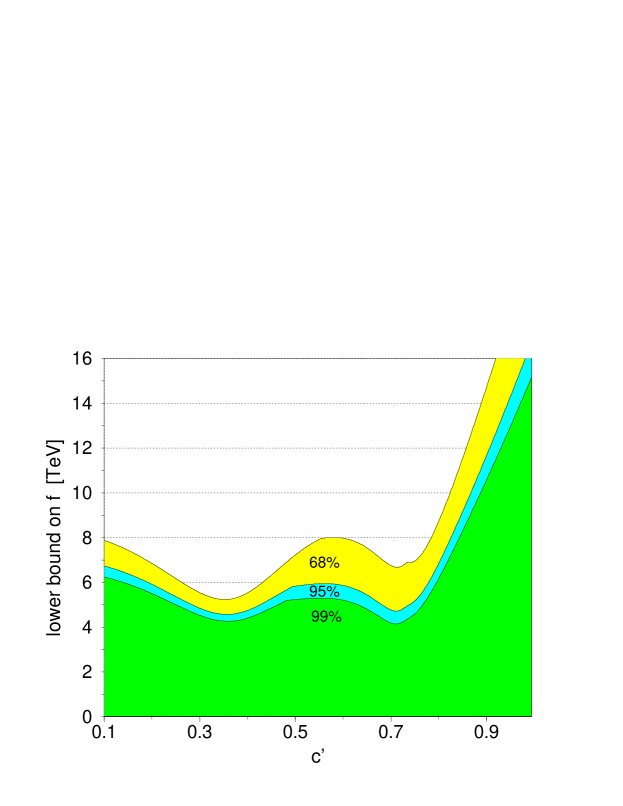
Figure 1: The region of parameters excluded to 68%, 95%, and 99% C.L. is shown as a function of $c^{\prime}$. The parameter $c$ was allowed to vary between $0.1<c<0.995$ for each $c^{\prime}$ to give the least restrictive bound on $f$. (See also Fig. 2.)

First consider the region of parameters relevant to the model. To ensure the high energy gauge couplings $g_{1,2},g^{\prime}_{1,2}$ are not strongly coupled, the angles $c=g/g_{2}$, $s=g/g_{1}$ $c^{\prime}=g^{\prime}/g^{\prime}_{2}$, $s^{\prime}=g^{\prime}/g^{\prime}_{1}$ cannot be too small. We conservatively allow for $c,s,c^{\prime},s^{\prime}>0.1$, or equivalently $0.1<c,c^{\prime}<0.995$. We allow $f$ to take on any value (although for small enough $f$ there will be constraints from direct production of $B_{H}$). The general procedure we used is to systematically step through values of $c$ and $c^{\prime}$, finding the lowest value of $f$ that leads to a shift in the $\chi^{2}$ corresponding to the 68%, 95%, and 99% confidence level (C.L.). For a three-parameter fit, this corresponds to a $\Delta\chi^{2}$ of about $3.5$, $7.8$, $11.3$ from the minimum, respectively. Globally, for any choice of high energy gauge couplings, we find

$$f>(4.1,\,4.6,\,5.2)\;{\rm TeV}\quad{\rm at}\quad(99\%,\,95\%,68\%)\;{\rm C.L.}$$ (5.3)

We used $m_{h}=115$ GeV, and verified that the bound is not lowered for larger values of the Higgs mass. Of course these bounds are saturated only for very specific values of the gauge couplings. The bound on $f$ is perhaps best illustrated as a function of $c^{\prime}$, which we do in Fig. 1. The shaded area below the lines shows the region of parameter space excluded by precision electroweak data. Note that we numerically found the value of $c$ that gave the least restrictive bound on $f$ for every $c^{\prime}$. For a specific choice of $c$ the bound on $f$ can be stronger. This is shown in Fig. 2

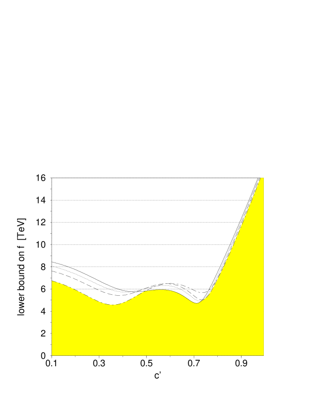
Figure 2: The region of parameters excluded to 95% C.L. is shown as a function of $c^{\prime}$. The region below the contours is excluded to 95% C.L. for $c$ equal to $0.1$ (solid), $0.5$ (dotted), $0.7$ (dashed), $0.99$ (dot-dashed). The shaded region is excluded for any choice of $c$.

where we show contours of the 95% excluded region for fixed $c$ while $c^{\prime}$ was allowed to vary. This figure makes it clear that the least restrictive bound is obtained for different values of $c$ as $c^{\prime}$ is varied. The shaded region is identical to the 95% C.L. region shown in Fig. 1, illustrating how the exclusion regions in Fig. 1 were obtained.

While we fit to 21 observables, inevitably certain observables are more sensitive to the new physics. To gain some insight into the main observables leading to the bounds shown in Figs. 1–2, we show in Fig. 3 the deviation of $\Gamma_{Z}$, $A^{b}_{FB}$,

Figure 3: The difference between the predicted and the experimentally measured values for four observables in standard deviations (the pull). In both figures the decay constant was fixed to $f=4$ TeV. The figure on the left (right) has a fixed $c=0.1$ ($c=0.99$); other values interpolate between these two figures. Notice that the observable that gives the largest contribution varies depending on $c^{\prime}$.

$A_{LR}$, and $Q_{W}$ from the experimental value (the pull) as a function of $c^{\prime}$ for fixed $f=4$ TeV and two choices of $c=0.1$ and $0.99$. A set of parameters is typically ruled out by the global fit once a single observable has a pull greater than of order $\pm 4$. The variation of $A^{b}_{FB}$ and $A_{LR}$ also explains the appearance in Figs. 1–2 of a rise in the bound on $f$ for small $c^{\prime}$ (where $A^{b}_{FB}$ is important) large $c^{\prime}$ (where many observables are important) and the bump in the middle (where $A_{LR}$ is important). Note that the region of large $c^{\prime}$ corresponds to the $U(1)_{1}$ gauge coupling (the gauge coupling of the quarks and leptons) getting strong.

We can now move on to discuss the fits done for reasonable values of the parameter $a$. We have redone the fit with $a=(0.1,0.5,1,2)$ and the results are displayed in Fig. 4. For generic couplings we see that the 95% C.L. bound is well above 4 TeV. However, for certain choices of the parameters the contribution from the triplet VEV can partially cancel against the gauge boson contributions accidentally. This happens near $c^{\prime}\sim 0.3$ when the triplet VEV, Eq. (4.22), is maximized which occurs when either

$$\frac{\lambda}{a(g_{1}^{2}+g_{1}^{\prime 2})}\sim 1\quad{\rm or}\quad\frac{\lambda}{a(g_{1}^{2}+g_{1}^{\prime 2})}\ll 1\;.$$ (5.4)

The first region corresponds to very small $a\sim 0.025$ where the triplet mass, Eq. (4.23), nearly vanishes. The second region corresponds to larger values of $a\mathrel{\>{\hbox{\raise 1.50696pt\hbox{$>$}}\kern-3.8889pt\kern-3.8889pt\hbox{\lower 2.79857pt\hbox{$\sim$}}}\>}1$, as illustrated by the bottom two figures. However, as pointed out in [3] the triplet VEV is naturally expected to be small, and we see from Fig. 4 that it is generically a sub-leading effect. The weakest bound, $f>4.0$ TeV, arises for $a=0.025$ or $a\mathrel{\>{\hbox{\raise 1.50696pt\hbox{$>$}}\kern-3.8889pt\kern-3.8889pt\hbox{\lower 2.79857pt\hbox{$\sim$}}}\>}1$. Another way to obtain an approximate bound is to redo the fit imposing a maximal triplet VEV, $\Delta^{\prime}=\Delta/16$, shown in Fig. 5. In general the real bound on $f$ could be stronger than what is found by this method, because the point corresponding to this bound might be eliminated by imposing the constraint of a positive triplet mass squared. This method gives a bound similar to that obtained from Figure 4 because at the lowest value of $f$ the triplet mass squared is positive. Similarly, one finds that the lower bound on the heavy gauge boson masses are: $M_{B_{H}}>650$ GeV and $M_{W_{H}}>2.7$ TeV.

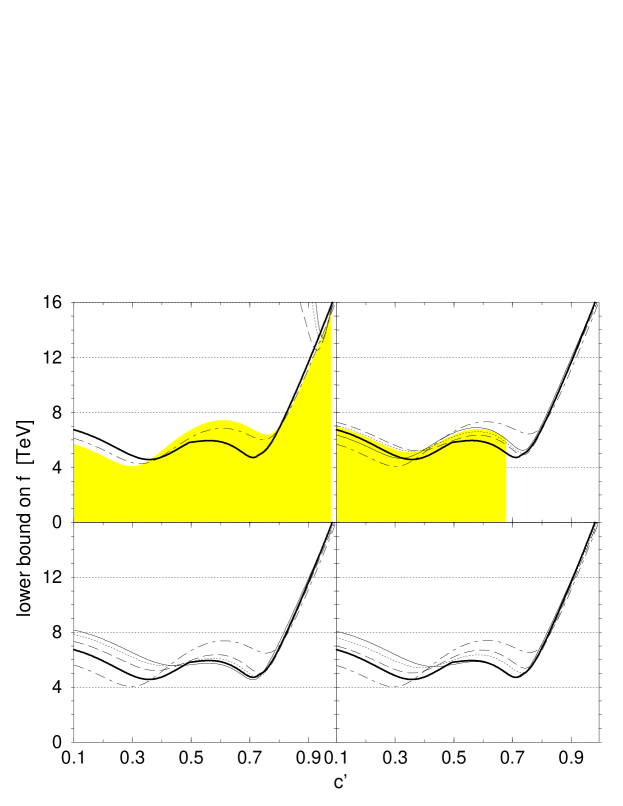
Figure 4: The region of parameters excluded to 95% C.L. is shown as a function of $c^{\prime}$. The four figures correspond to $a=0.1,0.5,1,2$ corresponding to top-left, top-right, bottom-left, and bottom-right. The region below the contours is excluded to 95% C.L. for $c$ equal to $0.1$ (solid), $0.5$ (dotted), $0.7$ (dashed), $0.99$ (dot-dashed). The heavy solid line displays the bound from Fig. 2. The shaded region corresponds to the extension of the excluded region obtained by requiring a positive triplet mass squared.

Figure 5: The region of parameters excluded to 95% C.L. is shown below the lines. The solid curve is for $\Delta^{\prime}=0$ as in Fig. 1, while the dashed curve is for $\Delta^{\prime}=\Delta/16$. The weakest bound at $c^{\prime}=0.29$ corresponds to $a=0.025$ [using Eq.(4.22)].

Given the above bound on the scale $f$ we can quantify the amount of fine-tuning in the model using the fine-tuning measure proposed in [3]. The contribution to the Higgs mass squared from the heavy partner of the top (with mass $m^{\prime}$) is

$$-\frac{3\lambda_{t}^{2}}{4\pi^{2}}m^{\prime 2}\log\frac{4\pi f}{m^{\prime}}~{}.$$ (5.5)

From the definition of $\lambda_{t}$ and $\lambda_{H}$ one can show that $m^{\prime}>\sqrt{2}f$, so with our bound on $f$ we have $m^{\prime}>5.7$ TeV, which for a 200 GeV Higgs implies a fine-tuning of 0.8%.

The generic reason for obtaining relatively strong constraints on the symmetry breaking scale in this model is that weak isospin is violated. In the SM there is an $SU(2)$ global symmetry (called “custodial” $SU(2)$) which protects the $\rho_{*}$ parameter from large corrections. These corrections in the SM can only come from custodial $SU(2)$ violating interactions like hypercharge and Yukawa couplings. The importance of custodial $SU(2)$ was noted in the early literature on composite Higgs models [9], and recently emphasized again in [7]. However, in the littlest Higgs model the heavy gauge bosons break custodial symmetry since the embeddings of $SU(2)_{1}$ and $SU(2)_{2}$ into $SU(5)$ as $\mathbf{5}\rightarrow(\mathbf{2},\mathbf{1})+(\mathbf{1},\mathbf{2})+(\mathbf{1},\mathbf{1})$ break all non-Abelian global symmetries acting on the Higgs. Interactions of these heavy gauge bosons shift observables from their standard model values. Indeed, we find that the $\rho_{*}$ parameter in (4.12) gets corrections of order $v^{2}/f^{2}$ independently of the mixing angles (even in the absence of a triplet VEV), therefore it is not hard to understand the bounds found above.

6 Conclusions

We have calculated the electroweak precision constraints on the littlest Higgs model, incorporating corrections resulting from heavy gauge boson exchange and the triplet VEV. Using a global fit to 21 observables, we found that generically throughout the parameter space the smallest symmetry breaking scale consistent with present experimental measurements is well above 4 TeV and for particular parameters the bound is $f>4.0$ TeV at 95% C.L, which implies that the Higgs mass squared is tuned to 0.8%. This bound arises for a specific choice of the high energy gauge couplings, roughly $a=0.025$, $c=g/g_{2}\sim 0.99$, and $c^{\prime}=g^{\prime}/g^{\prime}_{2}\sim 0.3$. The origin of the strong constraints on this model is the absence of a custodial $SU(2)$ symmetry, leading to large contributions to $\Delta\rho_{*}=\alpha T$, even in the absence of a triplet Higgs VEV. To the best of our knowledge, no little Higgs model constructed to date has a custodial $SU(2)$ symmetry, suggesting that similarly strong constraints are expected in other little Higgs models.

Appendix A: Predictions for Electroweak Observables

In this appendix we give the predictions for the shifts in the electroweak precision observables due to new tree-level physics beyond the SM in the $SU(5)/SO(5)$ littlest Higgs model. The electroweak observables depend on three parameters, $c,c^{\prime}$ and $\Delta$. Using the results given in [22, 25] we find the following results:

$$\Gamma_{Z} = \left(\Gamma_{Z}\right)_{SM}\left[1+\Delta(1.7-0.23c^{2}-0.89c^{4}-3.8c^{\prime 2}+0.83c^{\prime 4})-5.4\Delta^{\prime}\right]$$

$$R_{e} = \left(R_{e}\right)_{SM}\left[1+\Delta(0.34-0.18c^{2}+0.08c^{4}-3.0c^{\prime 2}+4.6c^{\prime 4})-1.1\Delta^{\prime}\right]$$

$$R_{\mu} = \left(R_{\mu}\right)_{SM}\left[1+\Delta(0.34-0.18c^{2}+0.08c^{4}-3.0c^{\prime 2}+4.6c^{\prime 4})-1.1\Delta^{\prime}\right]$$

$$R_{\tau} = \left(R_{\tau}\right)_{SM}\left[1+\Delta(0.34-0.18c^{2}+0.08c^{4}-3.0c^{\prime 2}+4.6c^{\prime 4})-1.1\Delta^{\prime}\right]$$

$$\sigma_{h} = \left(\sigma_{h}\right)_{SM}\left[1+\Delta(-0.04+0.02c^{2}+0.01c^{4}+0.31c^{\prime 2}-0.48c^{\prime 4})+0.12\Delta^{\prime}\right]$$

$$R_{b} = \left(R_{b}\right)_{SM}\left[1+\Delta(-0.08+0.04c^{2}-0.02c^{4}+0.66c^{\prime 2}-1.0c^{\prime 4})+0.24\Delta^{\prime}\right]$$

$$R_{c} = \left(R_{c}\right)_{SM}\left[1+\Delta(0.15-0.08c^{2}+0.04c^{4}-1.3c^{\prime 2}+1.9c^{\prime 4})-0.47\Delta^{\prime}\right]$$

$$A_{FB}^{e} = \left(A_{FB}^{e}\right)_{SM}+\Delta(0.73-0.38c^{2}+0.18c^{4}-6.4c^{\prime 2}+9.8c^{\prime 4})-2.3\Delta^{\prime}$$

$$A_{FB}^{\mu} = \left(A_{FB}^{\mu}\right)_{SM}+\Delta(0.73-0.38c^{2}+0.18c^{4}-6.4c^{\prime 2}+9.8c^{\prime 4})-2.3\Delta^{\prime}$$

$$A_{FB}^{\tau} = \left(A_{FB}^{\tau}\right)_{SM}+\Delta(0.73-0.38c^{2}+0.18c^{4}-6.4c^{\prime 2}+9.8c^{\prime 4})-2.3\Delta^{\prime}$$

$$A_{\tau}(P_{\tau}) = \left(A_{\tau}(P_{\tau})\right)_{SM}+\Delta(3.2-1.7c^{2}+0.78c^{4}-28c^{\prime 2}+43c^{\prime 4})-10\Delta^{\prime}$$

$$A_{e}(P_{\tau}) = \left(A_{e}(P_{\tau})\right)_{SM}+\Delta(3.2-1.7c^{2}+0.78c^{4}-28c^{\prime 2}+43c^{\prime 4})-10\Delta^{\prime}$$

$$A_{FB}^{b} = \left(A_{FB}^{b}\right)_{SM}+\Delta(2.3-1.2c^{2}+0.54c^{4}-20c^{\prime 2}+30c^{\prime 4})-7.2\Delta^{\prime}$$

$$A_{FB}^{c} = \left(A_{FB}^{c}\right)_{SM}+\Delta(1.8-0.91c^{2}+0.42c^{4}-15c^{\prime 2}+23c^{\prime 4})-5.6\Delta^{\prime}$$

$$A_{LR} = \left(A_{LR}\right)_{SM}+\Delta(3.2-1.7c^{2}+0.78c^{4}-28c^{\prime 2}+43c^{\prime 4})-10\Delta^{\prime}$$

$$M_{W} = \left(M_{W}\right)_{SM}\left[1+\Delta(0.89-0.21c^{2}+0.21c^{4}-3.6c^{\prime 2}+3.6c^{\prime 4})-2.9\Delta^{\prime}\right]$$

$$g_{L}^{2}(\nu N\rightarrow\nu X) = \left(g_{L}^{2}(\nu N\rightarrow\nu X)\right)_{SM}+\Delta(1.1-0.16c^{2}+0.25c^{4}-2.7c^{\prime 2}+1.2c^{\prime 4})$$

$$-3.4\Delta^{\prime}$$

$$g_{R}^{2}(\nu N\rightarrow\nu X) = \left(g_{R}^{2}(\nu N\rightarrow\nu X)\right)_{SM}+\Delta(-0.032+0.055c^{2}-0.085c^{4}+0.92c^{\prime 2}$$

$$-0.42c^{\prime 4})+0.10\Delta^{\prime}$$

$$g_{eV}(\nu e\rightarrow\nu e) = \left(g_{eV}(\nu e\rightarrow\nu e)\right)_{SM}+\Delta(-0.87+0.43c^{2}-0.66c^{4}+7.1c^{\prime 2}-3.3c^{\prime 4})$$

$$+2.8\Delta^{\prime}$$

$$g_{eA}(\nu e\rightarrow\nu e) = \left(g_{eA}(\nu e\rightarrow\nu e)\right)_{SM}-\frac{5\Delta}{8}+2\Delta^{\prime}$$

$$Q_{W}(Cs) = \left(Q_{W}(Cs)\right)_{SM}+\Delta(-1.5-47c^{2}+73c^{4}-786c^{\prime 2}+363c^{\prime 4})+4.7\Delta^{\prime}$$

We also give in Table (1) the experimental data [23, 27] and the SM predictions used for our fit.

Quantity	Experiment	SM($m_{h}=115$ GeV)
$\Gamma_{Z}$	2.4952 $\pm$ 0.0023	2.4965
$R_{e}$	20.804 $\pm$ 0.050	20.744
$R_{\mu}$	20.785 $\pm$ 0.033	20.744
$R_{\tau}$	20.764 $\pm$ 0.045	20.744
$\sigma_{h}$	41.541 $\pm$ 0.037	41.480
$R_{b}$	0.2165 $\pm$ 0.00065	0.2157
$R_{c}$	0.1719 $\pm$ 0.0031	0.1723
$A_{FB}^{e}$	0.0145 $\pm$ 0.0025	0.0163
$A_{FB}^{\mu}$	0.0169 $\pm$ 0.0013	0.0163
$A_{FB}^{\tau}$	0.0188 $\pm$ 0.0017	0.0163
$A_{\tau}(P_{\tau})$	0.1439 $\pm$ 0.0043	0.1475
$A_{e}(P_{\tau})$	0.1498 $\pm$ 0.0048	0.1475
$A_{FB}^{b}$	0.0994 $\pm$ 0.0017	0.1034
$A_{FB}^{c}$	0.0685 $\pm$ 0.0034	0.0739
$A_{LR}$	0.1513 $\pm$ 0.0021	0.1475
$M_{W}$	80.450 $\pm$ 0.034	80.389
$g_{L}^{2}(\nu N\rightarrow\nu X)$	0.3020 $\pm$ 0.0019	0.3039
$g_{R}^{2}(\nu N\rightarrow\nu X)$	0.0315 $\pm$ 0.0016	0.0301
$g_{eA}(\nu e\rightarrow\nu e)$	-0.507 $\pm$ 0.014	-0.5065
$g_{eV}(\nu e\rightarrow\nu e)$	-0.040 $\pm$ 0.015	-0.0397
$Q_{W}(Cs)$	-72.65 $\pm$ 0.44	-73.11

Table 1: The experimental results [23, 27] and the SM predictions for the various electroweak precision observables used for the fit. The SM predictions are for $m_{h}=115$ GeV and $\alpha_{s}=0.12$ and calculated [28] using GAPP [29].

References

• [1]
• [2] N. Arkani-Hamed, A. G. Cohen and H. Georgi, Phys. Lett. B 513, 232 (2001) [hep-ph/0105239].
• [3] N. Arkani-Hamed, A. G. Cohen, E. Katz and A. E. Nelson, JHEP 0207, 034 (2002) [hep-ph/0206021].
• [4] N. Arkani-Hamed, A. G. Cohen, E. Katz, A. E. Nelson, T. Gregoire and J. G. Wacker, JHEP 0208, 021 (2002) [hep-ph/0206020].
• [5] I. Low, W. Skiba and D. Smith, Phys. Rev. D 66, 072001 (2002) [hep-ph/0207243].
• [6] N. Arkani-Hamed, A. G. Cohen, T. Gregoire and J. G. Wacker, JHEP 0208, 020 (2002) [hep-ph/0202089]; K. Lane, Phys. Rev. D 65, 115001 (2002) [hep-ph/0202093]. T. Gregoire and J. G. Wacker, JHEP 0208, 019 (2002) [hep-ph/0206023]; hep-ph/0207164.
• [7] R. S. Chivukula, N. Evans and E. H. Simmons, Phys. Rev. D 66, 035008 (2002) [hep-ph/0204193].
• [8] H. Georgi and A. Pais, Phys. Rev. D 10, 539 (1974); Phys. Rev. D 12, 508 (1975).
• [9] D. B. Kaplan and H. Georgi, Phys. Lett. B 136, 183 (1984); D. B. Kaplan, H. Georgi and S. Dimopoulos, Phys. Lett. B 136, 187 (1984); H. Georgi, D. B. Kaplan and P. Galison, Phys. Lett. B 143, 152 (1984); M. J. Dugan, H. Georgi and D. B. Kaplan, Nucl. Phys. B 254, 299 (1985).
• [10] D. B. Kaplan and H. Georgi, Phys. Lett. B 145, 216 (1984).
• [11] M. Schmaltz, hep-ph/0210415.
• [12] N. S. Manton, Nucl. Phys. B 158, 141 (1979) P. Forgács and N. S. Manton, Commun. Math. Phys.  72, 15 (1980); S. Randjbar-Daemi, A. Salam and J. Strathdee, Nucl. Phys. B 214, 491 (1983); D. Kapetanakis and G. Zoupanos, Phys. Rept.  219, 1 (1992); G. R. Dvali, S. Randjbar-Daemi and R. Tabbash, Phys. Rev. D 65, 064021 (2002) [hep-ph/0102307].
• [13] Y. Hosotani, Phys. Lett. B 126, 309 (1983); Phys. Lett. B 129, 193 (1983); Annals Phys.  190, 233 (1989).
• [14] H. Hatanaka, T. Inami and C. S. Lim, Mod. Phys. Lett. A 13, 2601 (1998) [hep-th/9805067]; H. Hatanaka, Prog. Theor. Phys.  102, 407 (1999) [hep-th/9905100]; M. Kubo, C. S. Lim and H. Yamashita, hep-ph/0111327.
• [15] I. Antoniadis and K. Benakli, Phys. Lett. B 326, 69 (1994) [hep-th/9310151]; I. Antoniadis, K. Benakli and M. Quirós, Nucl. Phys. B 583, 35 (2000) [hep-ph/0004091]; I. Antoniadis, K. Benakli and M. Quirós, New J. Phys.  3, 20 (2001) [hep-th/0108005]; G. von Gersdorff, N. Irges and M. Quirós, Nucl. Phys. B 635, 127 (2002) [hep-th/0204223]; hep-ph/0206029; hep-ph/0210134.
• [16] L. J. Hall, Y. Nomura and D. R. Smith, Nucl. Phys. B 639, 307 (2002) [hep-ph/0107331]. G. Burdman and Y. Nomura, hep-ph/0210257.
• [17] C. Csáki, C. Grojean and H. Murayama, hep-ph/0210133.
• [18] H. Georgi, E. E. Jenkins and E. H. Simmons, Phys. Rev. Lett.  62, 2789 (1989) [Erratum-ibid.  63, 1540 (1989)]; Nucl. Phys. B 331, 541 (1990).
• [19] S. Dimopoulos and D. E. Kaplan, Phys. Lett. B 531, 127 (2002) [hep-ph/0201148].
• [20] R. S. Chivukula, E. H. Simmons and J. Terning, Phys. Lett. B 346, 284 (1995) [hep-ph/9412309].
• [21] C. Csáki, J. Erlich, G. D. Kribs and J. Terning, Phys. Rev. D 66, 075008 (2002) [hep-ph/0204109].
• [22] M. E. Peskin and T. Takeuchi, Phys. Rev. D 46, 381 (1992).
• [23] J. Erler and P. Langacker, review in “The Review of Particle Properties,” K. Hagiwara et al. [Particle Data Group Collaboration], Phys. Rev. D 66, 010001 (2002), updated version online: http://www-pdg.lbl.gov/2001/stanmodelrpp.ps.
• [24] D. C. Kennedy and B. W. Lynn, Nucl. Phys. B 322, 1 (1989); D. C. Kennedy, B. W. Lynn, C. J. Im and R. G. Stuart, Nucl. Phys. B 321, 83 (1989).
• [25] C. P. Burgess, S. Godfrey, H. Konig, D. London and I. Maksymyk, Phys. Rev. D 49, 6115 (1994) [hep-ph/9312291].
• [26] C. Csáki, J. Erlich and J. Terning, Phys. Rev. D 66, 064021 (2002) [hep-ph/0203034].
• [27] LEP Electroweak Working Group, LEPEWWG/2002-01,
http://lepewwg.web.cern.ch/LEPEWWG/stanmod/.
• [28] J. Erler, private communication.
• [29] J. Erler, hep-ph/0005084.