Abstract

We show that initial-state interactions contribute to the $\cos 2\phi$ distribution in unpolarized Drell-Yan lepton pair production $p\,p$ and $p\,\overline{p}\to\ell^{+}\ell^{-}X$, without suppression. The asymmetry is expressed as a product of chiral-odd distributions $h_{1}^{\perp}(x_{1},\mbox{\boldmath$p$}_{\perp}^{2})\times\overline{h}_{1}^{\perp}(x_{2},\mbox{\boldmath$k$}_{\perp}^{2})$, where the quark-transversity function $h_{1}^{\perp}(x,\mbox{\boldmath$p$}_{\perp}^{2})$ is the transverse momentum dependent, light-cone momentum distribution of transversely polarized quarks in an unpolarized proton. We compute this (naive) $T$-odd and chiral-odd distribution function and the resulting $\cos 2\phi$ asymmetry explicitly in a quark-scalar diquark model for the proton with initial-state gluon interaction. In this model the function $h_{1}^{\perp}(x,\mbox{\boldmath$p$}_{\perp}^{2})$ equals the $T$-odd (chiral-even) Sivers effect function $f^{\perp}_{1T}(x,\mbox{\boldmath$p$}_{\perp}^{2})$. This suggests that the single-spin asymmetries in the SIDIS and the Drell-Yan process are closely related to the $\cos 2\phi$ asymmetry of the unpolarized Drell-Yan process, since all can arise from the same underlying mechanism. This provides new insight regarding the role of quark and gluon orbital angular momentum as well as that of initial- and final-state gluon exchange interactions in hard QCD processes.

1 Introduction

Single-spin asymmetries in hadronic reactions have been among the most challenging phenomena to understand from basic principles in QCD. Several such asymmetries have been observed in experiment, and a number of theoretical mechanisms have been suggested [1, 2, 3, 4, 5, 6]. Recently, a new way of producing single-spin asymmetries in semi-inclusive deep inelastic scattering (SIDIS) and the Drell-Yan process has been put forward [7, 8]. It was shown that the exchange of a gluon, viewed as initial- or final-state interactions, could produce the necessary phase leading to a single transverse spin asymmetry. The main new feature is that despite the presence of an additional gluon, this asymmetry occurs without suppression by a large energy scale appearing in the process under consideration. It has been recognized since then [9], that this mechanism can be viewed as the so-called Sivers effect [1, 10], which was thought to be forbidden by time-reversal invariance [4]. Apart from generating Sivers effect asymmetries, the mechanism offers new insight regarding the role of orbital angular momentum of quarks in a hadron and their spin-orbit couplings; in fact, the same $\vec{S}\cdot\vec{L}$ matrix elements enter the anomalous magnetic moment of the proton [7]. The new mechanism for single target-spin asymmetries in SIDIS necessarily requires non-collinear quarks and gluons, and in the Sivers asymmetry the quarks carry no polarization on average. As such it is very different from mechanisms involving transversity (often denoted by $h_{1}$ or $\delta q$), which correlates the spin of the transversely polarized hadron with the transverse polarization of its quarks.

In further contrast, the exchange of a gluon can also lead to transversity of quarks inside an unpolarized hadron. This chiral-odd partner of the Sivers effect has been discussed in Refs. [6, 11], and in this paper we will show explicitly how initial-state interactions generate this effect. Goldstein and Gamberg reported recently that $h_{1}^{\perp}(x,\mbox{\boldmath$p$}_{\perp}^{2})$ is proportional to $f^{\perp}_{1T}(x,\mbox{\boldmath$p$}_{\perp}^{2})$ in the quark-scalar diquark model [12]. We confirm this and find that these two distribution functions are in fact equal in this model. Although this property is not expected to be satisfied in general, nevertheless, one may expect these functions to be comparable in magnitude, since both functions can be generated by the same mechanism. We investigate the consequences of the present model result for the unpolarized Drell-Yan process. We obtain an expression for the $\cos{2\phi}$ asymmetry in the lepton pair angular distribution. Here $\phi$ is the angle between the lepton plane and the plane of the incident hadrons in the lepton pair center of mass. This asymmetry was measured a long time ago [13, 14] and was found to be large. Several theoretical explanations (some of which will be briefly discussed below) have been put forward, but we will show that a natural explanation can come from initial-state interactions which are unsuppressed by the invariant mass of the lepton pair.

2 The unpolarized Drell-Yan process

The unpolarized Drell-Yan process cross section has been measured in pion-nucleon scattering: $\pi^{-}\,N\rightarrow\mu^{+}\,\mu^{-}\,X$, with $N$ deuterium or tungsten and a $\pi^{-}$-beam with energy of 140, 194, 286 GeV [13] and 252 GeV [14]. Conventionally the differential cross section is written as

$$\frac{1}{\sigma}\frac{d\sigma}{d\Omega}=\frac{3}{4\pi}\,\frac{1}{\lambda+3}\,\left(1+\lambda\cos^{2}\theta+\mu\sin^{2}\theta\cos\phi+\frac{\nu}{2}\sin^{2}\theta\cos 2\phi\right).$$ (1)

These angular dependencies can all be generated by perturbative QCD corrections, where for instance initial quarks radiate off high energy gluons into the final state. Such a perturbative QCD calculation at next-to-leading order leads to $\lambda\approx 1,\mu\approx 0,\nu\approx 0$ at very small transverse momentum of the lepton pair. More generally, the Lam-Tung relation $1-\lambda-2\nu=0$ [17] is expected to hold at order $\alpha_{s}$ and the relation is hardly modified by next-to-leading order ($\alpha_{s}^{2}$) perturbative QCD corrections [18]. However, this relation is not satisfied by the experimental data [13, 14]. The Drell-Yan data shows remarkably large values of $\nu$, reaching values of about 30% at transverse momenta of the lepton pair between 2 and 3 GeV (for $Q^{2}=m_{\gamma^{*}}^{2}=(4-12\,\hbox{GeV})^{2}$ and extracted in the Collins-Soper frame [19] to be discussed below). These large values of $\nu$ are not compatible with $\lambda\approx 1$ as also seen in the data.

A number of explanations have been put forward, such as a higher twist effect [20, 21], following the ideas of Berger and Brodsky [22]. In Ref. [20] the higher twist effect is modeled using an asymptotic pion distribution amplitude, and it appears to fall short in explaining the large values of $\nu$.

In Ref. [18] factorization-breaking correlations between the incoming quarks are assumed and modeled in order to account for the large $\cos 2\phi$ dependence. Here the correlations are both in the transverse momentum and the spin of the quarks. In Ref. [6] this idea was applied in a factorized approach [23] involving the chiral-odd partner of the Sivers effect, which is the transverse momentum dependent distribution function called $h_{1}^{\perp}$. From this point of view, the large $\cos 2\phi$ azimuthal dependence can arise at leading order, i.e. it is unsuppressed, from a product of two such distribution functions. It offers a natural explanation for the large $\cos 2\phi$ azimuthal dependence, but at the same time also for the small $\cos\phi$ dependence, since chiral-odd functions can only occur in pairs. The function $h_{1}^{\perp}$ is a quark helicity-flip matrix element and must therefore occur accompanied by another helicity flip. In the unpolarized Drell-Yan process this can only be a product of two $h_{1}^{\perp}$ functions. Since this implies a change by two units of angular momentum, it does not contribute to a $\cos\phi$ asymmetry. In the present paper we will discuss this scenario in terms of initial-state interactions, which can generate a nonzero function $h_{1}^{\perp}$.

We would also like to point out the experimental observation that the $\cos 2\phi$ dependence as observed by the NA10 collaboration does not seem to show a strong dependence on $A$, i.e. there was no significant difference between the deuterium and tungsten targets. Hence, it is unlikely that the asymmetry originates from nuclear effects, and we shall assume it to be associated purely with hadronic effects. We refer to Ref. [24] for investigations of nuclear enhancements.

We compute the function $h_{1}^{\perp}(x,\mbox{\boldmath$p$}_{\perp}^{2})$ and the resulting $\cos 2\phi$ asymmetry explicitly in a quark-scalar diquark model for the proton with an initial-state gluon interaction. In this model $h_{1}^{\perp}(x,\mbox{\boldmath$p$}_{\perp}^{2})$ equals the $T$-odd (chiral-even) Sivers effect function $f^{\perp}_{1T}(x,\mbox{\boldmath$p$}_{\perp}^{2})$. Hence, assuming the $\cos 2\phi$ asymmetry of the unpolarized Drell-Yan process does arise from nonzero, large $h_{1}^{\perp}$, this asymmetry is expected to be closely related to the single-spin asymmetries in the SIDIS and the Drell-Yan process, since each of these effects can arise from the same underlying mechanism.

The Tevatron and RHIC should both be able to investigate azimuthal asymmetries such as the $\cos 2\phi$ dependence. Since polarized proton beams are available, RHIC will be able to measure single-spin asymmetries as well. Unfortunately, one might expect that the $\cos 2\phi$ dependence in $p\,p\rightarrow\ell\,\overline{\ell}\,X$ (measurable at RHIC) is smaller than for the process $\pi^{-}\,N\rightarrow\mu^{+}\,\mu^{-}\,X$, since in the former process there are no valence antiquarks present. In this sense, the cleanest extraction of $h_{1}^{\perp}$ would be from $p\,\overline{p}\rightarrow\ell\,\overline{\ell}\,X$.

3 Cross section calculation

In this section we will assume nonzero $h_{1}^{\perp}$ and discuss the calculation of the leading order unpolarized Drell-Yan cross section (given in Ref. [6] with slightly different notation)

$$\frac{d\sigma(h_{1}h_{2}\to\ell\overline{\ell}X)}{d\Omega dx_{1}dx_{2}d^{2}{\mbox{\boldmath$q$}_{\perp}}}=\frac{\alpha^{2}}{3Q^{2}}\;\sum_{a,\overline{a}}e_{a}^{2}\;\Bigg{\{}A(y)\;{\cal F}\left[f_{1}\overline{f}_{1}\right]$$ (2)

$$\mbox{}\qquad+B(y)\cos(2\phi)\;{\cal F}\left[\left(2\,\mbox{\boldmath$\hat{h}$}\!\cdot\!\mbox{\boldmath$p$}_{\perp}\,\,\mbox{\boldmath$\hat{h}$}\!\cdot\!\mbox{\boldmath$k$}_{\perp}\,-\,\mbox{\boldmath$p$}_{\perp}\!\cdot\!\mbox{\boldmath$k$}_{\perp}\,\right)\frac{h_{1}^{\perp}\overline{h}_{1}^{\perp}}{M_{1}M_{2}}\right]\Bigg{\}}.$$

This is expressed in the so-called Collins-Soper frame [19], for which one chooses the following set of normalized vectors (for details see e.g. [25]):

$$\hat{t} \equiv q/Q,$$ (3)

$$\hat{z} \equiv \frac{x_{1}}{Q}\tilde{P_{1}}-\frac{x_{2}}{Q}\tilde{P_{2}},$$ (4)

$$\hat{h} \equiv q_{\perp}/Q_{\perp}=(q-x_{1}\,P_{1}-x_{2}\,P_{2})/Q_{\perp},$$ (5)

where $\tilde{P_{i}}\equiv P_{i}-q/(2x_{i})$, $P_{i}$ are the momenta of the two incoming hadrons and $q$ is the four momentum of the virtual photon or, equivalently, of the lepton pair. This can be related to standard Sudakov decompositions of these momenta

$$P_{1}^{\mu} \equiv \frac{Q}{2x_{1}}\,\overline{n}^{\mu}+\frac{x_{1}M_{1}^{2}}{2Q}\,n^{\mu},$$ (6)

$$P_{2}^{\mu} \equiv \frac{x_{2}M_{2}^{2}}{2Q}\,\overline{n}^{\mu}+\frac{Q}{2x_{2}}\,n^{\mu},$$ (7)

$$q^{\mu} \equiv \frac{Q}{2}\,\overline{n}^{\mu}+\frac{Q}{2}\,n^{\mu}+q_{\perp}^{\mu},$$ (8)

with $Q_{\perp}^{2}\equiv-q_{\perp}^{2}\equiv\mbox{\boldmath$q$}_{\perp}^{2}\ll Q^{2}$, via the identification of the light-like vectors

$$\overline{n}^{\mu} = \left[\hat{t}^{\mu}+\hat{z}^{\mu}-\,\frac{Q_{\perp}}{Q}\hat{h}^{\mu}\right],$$ (9)

$$n^{\mu} = \left[\hat{t}^{\mu}-\hat{z}^{\mu}-\,\frac{Q_{\perp}}{Q}\,\hat{h}^{\mu}\right].$$ (10)

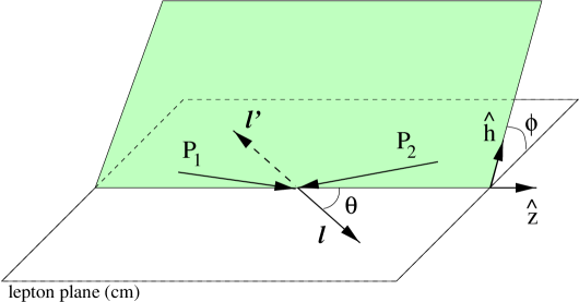
The azimuthal angles lie inside the plane orthogonal to $t$ and $z$. In particular, $d\Omega$ = $2dy\,d\phi^{l}$, where $\phi^{l}$ gives the orientation of $\hat{l}_{\perp}^{\mu}\equiv\left(g^{\mu\nu}-\hat{t}^{\mu}\hat{t}^{\nu}+\hat{z}^{\mu}\hat{z}^{\nu}\right)l_{\nu}$, the perpendicular part of the lepton momentum $l$; $\phi$ is the angle between $\hat{h}$ (the direction of $\mbox{\boldmath$q$}_{\perp}$) and $\hat{l}_{\perp}$. In the cross sections we also encounter the following functions of $y=l^{-}/q^{-}$, which in the lepton center of mass frame equals $y=(1+\cos\theta)/2$, where $\theta$ is the angle of the momentum of the outgoing lepton $l$ with respect to $\hat{z}$ (cf. Fig. 1):

$$A(y) = \left(\frac{1}{2}-y+y^{2}\right)\stackrel{{\scriptstyle cm}}{{=}}\frac{1}{4}\left(1+\cos^{2}\theta\right),$$ (11)

$$B(y) = y\,(1-y)\stackrel{{\scriptstyle cm}}{{=}}\frac{1}{4}\sin^{2}\theta.$$ (12)

Furthermore, we use the convolution notation

$${\cal F}\left[f\overline{f}\,\right]\equiv\;\int d^{2}\mbox{\boldmath$p$}_{\perp}\;d^{2}\mbox{\boldmath$k$}_{\perp}\;\delta^{2}(\mbox{\boldmath$p$}_{\perp}+\mbox{\boldmath$k$}_{\perp}-\mbox{\boldmath$q$}_{\perp})f^{a}(\Delta,\mbox{\boldmath$p$}_{\perp}^{2})\overline{f}{}^{a}(\overline{\Delta},\mbox{\boldmath$k$}_{\perp}^{2}),$$ (13)

where $\Delta,\overline{\Delta}$ are lightcone momentum fractions and $a$ is the flavor index.

Figure 1: Kinematics of the Drell-Yan process in the lepton center of mass frame.

In order to obtain the cross section expression one contracts the lepton tensor with the hadron tensor [6, 23]

$${\cal W}^{\mu\nu}=\frac{1}{3}\int dp^{-}dk^{+}d^{2}\mbox{\boldmath$p$}_{\perp}d^{2}\mbox{\boldmath$k$}_{\perp}\,\delta^{2}(\mbox{\boldmath$p$}_{\perp}+\mbox{\boldmath$k$}_{\perp}-\mbox{\boldmath$q$}_{\perp})\,\left.\hbox{Tr}\left(\Phi(p)\,\gamma^{\mu}\,\overline{\Phi}(k)\,\gamma^{\nu}\right)\right|_{p^{+},\,k^{-}}+\left(\begin{array}[]{c}q\leftrightarrow-q\\ \mu\leftrightarrow\nu\end{array}\right),$$ (14)

where $p^{+}=\Delta P_{1}^{+}=\Delta q^{+}/x_{1},\,k^{-}=\overline{\Delta}P_{2}^{-}=\overline{\Delta}q^{-}/x_{2}$. The correlation function $\Phi$ is parameterized in terms of the transverse momentum dependent quark distribution functions [11]

$$\Phi(\Delta,{\mbox{\boldmath$r$}}_{\perp};P,S)$$

$$= {M\over 2P^{+}}{\Big{[}}f_{1}(\Delta,{\mbox{\boldmath$r$}}_{\perp}){{\mbox{$\not\!P$}}\over M}+f_{1T}^{\perp}(\Delta,{\mbox{\boldmath$r$}}_{\perp}){\epsilon}_{\mu\nu\rho\sigma}{\gamma}^{\mu}{P^{\nu}r_{\perp}^{\rho}S_{T}^{\sigma}\over M^{2}}-g_{1s}(\Delta,{\mbox{\boldmath$r$}}_{\perp}){{\mbox{$\not\!P$}}{\gamma}_{5}\over M}$$

$$-h_{1T}(\Delta,{\mbox{\boldmath$r$}}_{\perp}){i{\sigma}_{\mu\nu}{\gamma}_{5}S_{T}^{\mu}P^{\nu}\over M}-h_{1s}^{\perp}(\Delta,{\mbox{\boldmath$r$}}_{\perp}){i{\sigma}_{\mu\nu}{\gamma}_{5}r_{\perp}^{\mu}P^{\nu}\over M^{2}}+h_{1}^{\perp}(\Delta,{\mbox{\boldmath$r$}}_{\perp}){{\sigma}_{\mu\nu}r_{\perp}^{\mu}P^{\nu}\over M^{2}}{\Big{]}}\ ,$$

and similarly for $\overline{\Phi}$.

We end this section by giving the resulting expression for $\nu$ [6]

$$\nu=2\sum_{a,\overline{a}}e_{a}^{2}\,{\cal F}\left[\left(2\,\mbox{\boldmath$\hat{h}$}\!\cdot\!\mbox{\boldmath$p$}_{\perp}\,\,\mbox{\boldmath$\hat{h}$}\!\cdot\!\mbox{\boldmath$k$}_{\perp}\,-\,\mbox{\boldmath$p$}_{\perp}\!\cdot\!\mbox{\boldmath$k$}_{\perp}\,\right)\frac{h_{1}^{\perp}\overline{h}_{1}^{\perp}}{M_{1}M_{2}}\right]\Bigg{/}\sum_{a,\overline{a}}e_{a}^{2}\,{\cal F}\left[f_{1}\overline{f}_{1}\right].$$ (16)

4 Asymmetry calculation

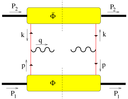
The above cross section in terms of $\Phi$ and $\overline{\Phi}$ can be represented by the diagram in Fig. 3.

Figure 2: The leading order contribution to the Drell-Yan process

.

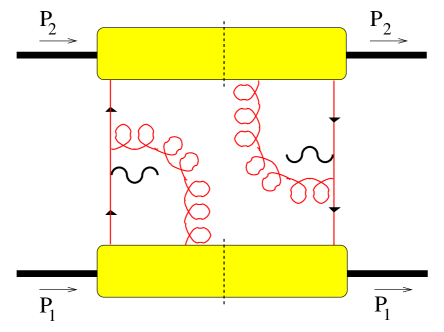
Figure 3: The initial-state interaction contribution to the Drell-Yan process.

Insertion of the parameterization of $\Phi$ and $\overline{\Phi}$ will yield the $\cos 2\phi$ asymmetry, among many other terms. However, in the lowest order quark-scalar diquark model the diagram Fig. 3 will not lead to nonzero $h_{1}^{\perp}$ in $\Phi$, and consequently, also not to a nonzero $\cos 2\phi$ asymmetry. To generate such an asymmetry we will include initial-state interactions corresponding to diagrams such as those depicted in Fig. 3. Following the reasoning of Refs. [9, 26], this should be equivalent to Fig. 3 with an effective $\Phi$ (and $\overline{\Phi}$) with nonzero $h_{1}^{\perp}$ function. Here we do not intend to give a full demonstration of this in the Drell-Yan process; a generalized factorization theorem which includes transverse momentum dependent functions and initial/final-state interactions remains to be proven [27]. Instead we present how to arrive at an effective $\Phi$ from initial/final-state interactions and use this effective $\Phi$ in Fig. 3. Also, for simplicity we will perform the explicit calculation in QED. Our analysis can be generalized to the corresponding calculation in QCD. The final-state interaction from gluon exchange has the strength ${|e_{1}e_{2}|\over 4\pi}\to C_{F}\alpha_{s}(\mu^{2})$, where $e_{i}$ are the photon couplings to the quark and diquark.

The diagram in Fig. 3 coincides with Fig. 6(a) of Ref. [28] used for the evaluation of a twist-4 contribution ($\sim 1/Q^{2}$) to the unpolarized Drell-Yan cross section. The differences compared to Ref. [28] are that in the present case there is nonzero transverse momentum of the partons, and the assumption that the matrix elements are nonvanishing in case the gluon has vanishing light-cone momentum fraction (but nonzero transverse momentum). This results in an unsuppressed asymmetry which is a function of the transverse momentum $Q_{\perp}$ of the lepton pair with respect to the initial hadrons. If this transverse momentum is integrated over, then the unsuppresed asymmetry will average to zero and the diagrams will only contribute at order $1/Q^{2}$ as in Ref. [28].

First we will calculate the $\Phi$ matrix to lowest order (called $\Phi_{L}^{\alpha\beta}$) in the quark-scalar diquark model which was used in Ref. [7]. (Although the model is based on a point-like coupling of a scalar diquark to elementary fermions, it can be softened to simulate a hadronic bound state by differentiating the wavefunction formally with respect to a parameter such as the proton mass.) As indicated earlier, no nonzero $f_{1T}^{\perp}$ and $h_{1}^{\perp}$ will arise from $\Phi_{L}^{\alpha\beta}$. Next we will include an additional gluon exchange to model the initial/final-state interactions (relevant for timelike/spacelike processes) to calculate $\Phi_{I/F}^{\alpha\beta}$ and do obtain nonzero values for $f_{1T}^{\perp}$ and $h_{1}^{\perp}$. Our results agree with those recently obtained in the same model by Goldstein and Gamberg [12]. We can then obtain an expression for the $\cos 2\phi$ asymmetry from Eq. (16) and perform a numerical estimation of the asymmetry.

4.1 $\Phi$ matrix in the lowest order ($\Phi_{L}^{\alpha\beta}$)

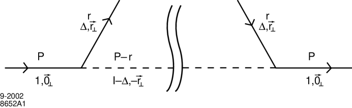
As indicated in Fig. 4 the initial proton has its momentum given by $P^{\mu}=(P^{+},P^{-},{\mbox{\boldmath$P$}}_{\perp})=(P^{+},{M^{2}\over P^{+}},{\mbox{\boldmath$0$}}_{\perp})$, and the final diquark ${P^{\prime}}^{\mu}=({P^{\prime}}^{+},{P^{\prime}}^{-},{\mbox{\boldmath$P$}}^{\prime}_{\perp})=(P^{+}(1-\Delta),{{\lambda}^{2}+{\mbox{\boldmath$r$}}_{\perp}^{2}\over P^{+}(1-\Delta)},{\mbox{\boldmath$r$}}_{\perp})$. We use the convention $a^{\pm}=a^{0}\pm a^{3}$, $a\cdot b={1\over 2}(a^{+}b^{-}+a^{-}b^{+})-{\mbox{\boldmath$a$}}_{\perp}\cdot{\mbox{\boldmath$b$}}_{\perp}$.

Figure 4: Diagram which gives the lowest order $\Phi$ (called $\Phi_{L}^{\alpha\beta}$.

We will first calculate the $\Phi$ matrix to lowest order ($\Phi_{L}^{\alpha\beta}$) in the quark-scalar diquark model used in Ref. [7]. By calculation of Fig. 4 one readily obtains

$$\Phi_{L}^{\alpha\beta} = ag^{2}{\Big{[}}{\overline{u}}(P,S){{\mbox{$\not\!r$}}+m\over r^{2}-m^{2}}{\Big{]}}^{\beta}{\Big{[}}{{\mbox{$\not\!r$}}+m\over r^{2}-m^{2}}{u}(P,S){\Big{]}}^{\alpha}\ {1\over P^{+}(1-\Delta)}$$

$$= ag^{2}{\Big{[}}{\overline{u}}(P,S)({\mbox{$\not\!r$}}+m){\Big{]}}^{\beta}{\Big{[}}({\mbox{$\not\!r$}}+m){u}(P,S){\Big{]}}^{\alpha}\ {1\over P^{+}(1-\Delta)}\$$

$$\times\Bigl{(}{1\over\Delta(M^{2}-{m^{2}+{\mbox{\boldmath$r$}}_{\perp}^{\,2}\over\Delta}-{\lambda^{2}+{\mbox{\boldmath$r$}}_{\perp}^{\,2}\over 1-\Delta})}{\Bigr{)}}^{2}\ ,$$

with a constant $a=1/(2(2\pi)^{3})$. The normalization is fixed by the condition

$$\int\ d\Delta\ d^{2}{\mbox{\boldmath$r$}}_{\perp}\ f_{1}(\Delta,{\mbox{\boldmath$r$}}_{\perp})\ =\ 1\ .$$ (18)

In Eq. (4.1) we used the relation

$$r^{2}-m^{2} = r^{+}(r^{-}-{m^{2}+{\mbox{\boldmath$r$}}_{\perp}^{\,2}\over r^{+}})\ =\ r^{+}(P^{-}-{\lambda^{2}+{\mbox{\boldmath$r$}}_{\perp}^{\,2}\over(1-\Delta)P^{+}}-{m^{2}+{\mbox{\boldmath$r$}}_{\perp}^{\,2}\over r^{+}})$$ (19)

$$= \Delta(M^{2}-{\lambda^{2}+{\mbox{\boldmath$r$}}_{\perp}^{\,2}\over 1-\Delta}-{m^{2}+{\mbox{\boldmath$r$}}_{\perp}^{\,2}\over\Delta})\ .$$

This model is similar to the so-called spectator model (see e.g. Ref. [29]), where in addition a vector diquark is included and the coupling constant $g$ is treated as a form factor (in order to guarantee convergence). Of course, this can be assumed in the present model calculation as well and will be discussed in Section 4.4. Assuming real form factors, the functions $f_{1T}^{\perp}$ and $h_{1}^{\perp}$ are strictly zero in the spectator model.

4.1.1 Calculation of $f_{1}(\Delta,{\mbox{\boldmath$r$}}_{\perp})$

For the calculation of the denominator of the asymmetry one needs to know the function $f_{1}(\Delta,{\mbox{\boldmath$r$}}_{\perp})$, which can be obtained from $\Phi^{\alpha\beta}$ given in Eq. (3):

$$f_{1}(\Delta,{\mbox{\boldmath$r$}}_{\perp})={1\over 2}\sum_{\pm S}{1\over 2}\Phi^{\alpha\beta}(\gamma^{+})^{\beta\alpha}\ .$$ (20)

We now take $\Phi=\Phi_{L}$ and for the numerator spinor contraction, we calculate

$${1\over 2}\sum_{\pm S}{\Big{[}}{\overline{u}}(P,S)({\mbox{$\not\!r$}}+m){\Big{]}}^{\beta}{\Big{[}}({\mbox{$\not\!r$}}+m){u}(P,S){\Big{]}}^{\alpha}\ (\gamma^{+})^{\beta\alpha}$$ (21)

$$= {1\over 2}{\rm Tr}\Big{[}({\mbox{$\not\!P$}}+M)({\mbox{$\not\!r$}}+m)\gamma^{+}({\mbox{$\not\!r$}}+m)\Big{]}$$

$$= 2P^{+}\Big{[}{\mbox{\boldmath$r$}}_{\perp}^{\,2}+(\Delta M+m)^{2}\Big{]}\ .$$

Then, from Eqs. (4.1), (20) and (21), we arrive at

$$f_{1}(\Delta,{\mbox{\boldmath$r$}}_{\perp}) = ag^{2}\ \Big{[}{\mbox{\boldmath$r$}}_{\perp}^{\,2}+(\Delta M+m)^{2}\Big{]}\ \ {1\over(1-\Delta)}\ \Bigl{(}{1\over\Delta(M^{2}-{m^{2}+{\mbox{\boldmath$r$}}_{\perp}^{\,2}\over\Delta}-{\lambda^{2}+{\mbox{\boldmath$r$}}_{\perp}^{\,2}\over 1-\Delta})}{\Bigr{)}}^{2}$$ (22)

$$= {g^{2}\over 2(2\pi)^{3}}\ {(1-\Delta)\ \Big{[}{\mbox{\boldmath$r$}}_{\perp}^{\,2}+(\Delta M+m)^{2}\Big{]}\over({\mbox{\boldmath$r$}}_{\perp}^{\,2}+B)^{2}}\ =\ C\frac{{\mbox{\boldmath$r$}}_{\perp}^{\,2}+D}{({\mbox{\boldmath$r$}}_{\perp}^{\,2}+B)^{2}},$$

where we define $C\equiv g^{2}(1-\Delta)/(2(2\pi)^{3})$, $D\equiv(\Delta M+m)^{2}$ and

$$B\ \equiv\ \Delta(1-\Delta)(-M^{2}+{m^{2}\over\Delta}+{\lambda^{2}\over 1-\Delta})\ .$$ (23)

Since we consider the proton state with mass $M$ as a bound state composed of a quark with mass $m$ and a diquark with mass $\lambda$, the function $B$ as given in Eq. (23) is always nonzero and positive.The integral in Eq. (18) with $f_{1}(\Delta,{\mbox{\boldmath$r$}}_{\perp})$ given in Eq. (22) can for instance be regulated by assuming a cutoff in the invariant mass: ${\cal M}^{2}=\sum_{i}{{\mbox{\boldmath$k$}}^{2}_{\perp i}+m^{2}_{i}\over x_{i}}<\Lambda^{2}$, and the value of $g^{2}$ is adjusted to satisfy the normalization condition Eq. (18) [30].

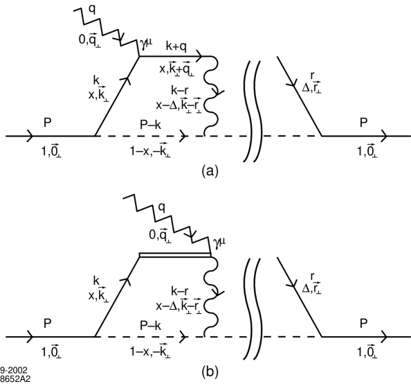
4.2 $\Phi$ matrix with final-state interaction ($\Phi_{F}^{\alpha\beta}$)

In order to obtain the $\Phi$ matrix with final-state interaction (called $\Phi_{F}^{\alpha\beta}$), from which one can trivially obtain the one with initial-state interaction, we calculate the diagram given in Fig. 5(b). This is equal to the diagram calculated by Ji and Yuan [31] to obtain nonzero $f_{1T}^{\perp}$, starting from the formal gauge invariant definition of this transverse momentum dependent distribution function [9, 26]. In Fig. 5(b) we attached the virtual photon line to the later end of the eikonal line in order to emphasize that the final-state interaction effect has become an ingredient of the distribution functions of the target proton. In reality, the whole eikonal line should be considered to be at the same point.

Figure 5: Diagrams which yield $\Phi$ with final-state interaction ($\Phi_{F}^{\alpha\beta})$.

Defining $\Phi_{F}^{\alpha\beta}$ through Fig. 5(b) (in the Feynman gauge), we have

$$\Phi_{F}^{\alpha\beta}$$

$$= iag^{2}\ e_{1}e_{2}\ \int{d^{4}k\over(2\pi)^{4}}\ {1\over 2}\ {-P^{+}((1-x)+(1-\Delta))\over P^{+}(1-\Delta)}$$

$$\times{2\over P^{+}((x-\Delta)+i\epsilon)}$$

$$\times{{\Big{[}}{\overline{u}}(P,S)({\mbox{$\not\!r$}}+m){\Big{]}}^{\beta}{\Big{[}}({\mbox{$\not\!k$}}+m){u}(P,S){\Big{]}}^{\alpha}\over(k^{2}-m^{2}+i\epsilon)((k-r)^{2}-\lambda_{g}^{2}+i\epsilon)((k-P)^{2}-\lambda^{2}+i\epsilon)}\ {1\over r^{2}-m^{2}}$$

$$+\ ({\rm h.c.})$$

$$= -iag^{2}\ e_{1}e_{2}\ \int{d^{2}{\mbox{\boldmath$k$}}_{\perp}\over 2(2\pi)^{4}}\int P^{+}dx\ {1\over P^{+3}\ x\ (x-\Delta)\ (1-x)}\ {(-(1-x)-(1-\Delta))\over 2P^{+}(1-\Delta)}$$

$$\times{2\over((x-\Delta)+i\epsilon)}\ {1\over\Delta(M^{2}-{m^{2}+{\mbox{\boldmath$r$}}_{\perp}^{\,2}\over\Delta}-{\lambda^{2}+{\mbox{\boldmath$r$}}_{\perp}^{\,2}\over 1-\Delta})}$$

$$\times\int dk^{-}{\Big{[}}{\overline{u}}(P,S)({\mbox{$\not\!r$}}+m){\Big{]}}^{\beta}{\Big{[}}({\mbox{$\not\!k$}}+m){u}(P,S){\Big{]}}^{\alpha}$$

$$\times{1\over\left(k^{-}-{(m^{2}+{\mbox{\boldmath$k$}}_{\perp}^{2})-i\epsilon\over xP^{+}}\right)\left((k^{-}-r^{-})-{(\lambda_{g}^{2}+({\mbox{\boldmath$k$}}_{\perp}-{\mbox{\boldmath$r$}}_{\perp})^{2})-i\epsilon\over(x-\Delta)P^{+}}\right)\left((k^{-}-P^{-})+{(\lambda^{2}+{\mbox{\boldmath$k$}}_{\perp}^{2})-i\epsilon\over(1-x)P^{+}}\right)}$$

$$+\ ({\rm h.c.})\ ,$$

where we used $k^{+}=xP^{+}.$ The derivation of the starting formula of Eq. (4.2) is given in the Appendix. This underlies the step from Fig. 5(a) to Fig. 5(b) and hence the step from Fig. 3 to Fig. 3.

For $\Phi_{F}^{\alpha\beta}$ in Eq. (4.2), we consider only the contribution from the imaginary part of ${1\over((x-\Delta)+i\epsilon)}$, that is, the contribution from $-i\pi\delta(x-\Delta)$. There is no contribution from the real part of ${1\over((x-\Delta)+i\epsilon)}$, since the hermitian conjugate term cancels it. Then, we have

$$\Phi_{F}^{\alpha\beta}$$

$$= 4\ (-iag^{2}\ e_{1}e_{2})\ \int{d^{2}{\mbox{\boldmath$k$}}_{\perp}\over 2(2\pi)^{4}}\int P^{+}dx\ {1\over P^{+3}\ x\ (x-\Delta)\ (1-x)}\ {(-(1-x)-(1-\Delta))\over 2P^{+}(1-\Delta)}$$

$$\times\Big{[}-i\pi\delta(x-\Delta)\Big{]}\ {1\over\Delta(M^{2}-{m^{2}+{\mbox{\boldmath$r$}}_{\perp}^{\,2}\over\Delta}-{\lambda^{2}+{\mbox{\boldmath$r$}}_{\perp}^{\,2}\over 1-\Delta})}$$

$$\times\int dk^{-}{\Big{[}}{\overline{u}}(P,S)({\mbox{$\not\!r$}}+m){\Big{]}}^{\beta}{\Big{[}}({\mbox{$\not\!k$}}+m){u}(P,S){\Big{]}}^{\alpha}$$

$$\times{1\over\left(k^{-}-{(m^{2}+{\mbox{\boldmath$k$}}_{\perp}^{2})-i\epsilon\over xP^{+}}\right)\left((k^{-}-r^{-})-{(\lambda_{g}^{2}+({\mbox{\boldmath$k$}}_{\perp}-{\mbox{\boldmath$r$}}_{\perp})^{2})-i\epsilon\over(x-\Delta)P^{+}}\right)\left((k^{-}-P^{-})+{(\lambda^{2}+{\mbox{\boldmath$k$}}_{\perp}^{2})-i\epsilon\over(1-x)P^{+}}\right)}\ .$$

When we perform the $k^{-}$ integration, we have

$$\Phi_{F}^{\alpha\beta}$$

$$= 4\ \pi\ ag^{2}\ e_{1}e_{2}\ \int{d^{2}{\mbox{\boldmath$k$}}_{\perp}\over 2(2\pi)^{4}}\int dx\ {1\over P^{+3}\ x\ (x-\Delta)\ (1-x)}\ {((1-x)+(1-\Delta))\over 2(1-\Delta)}$$

$$\times\delta(x-\Delta)\ {1\over\Delta(M^{2}-{m^{2}+{\mbox{\boldmath$r$}}_{\perp}^{\,2}\over\Delta}-{\lambda^{2}+{\mbox{\boldmath$r$}}_{\perp}^{\,2}\over 1-\Delta})}$$

$$\times{\Big{[}}{\overline{u}}(P,S)({\mbox{$\not\!r$}}+m){\Big{]}}^{\beta}{\Big{[}}({\mbox{$\not\!k$}}+m){u}(P,S){\Big{]}}^{\alpha}$$

$$\times 2\pi i\ {1\over\left(P^{-}-{(\lambda^{2}+{\mbox{\boldmath$k$}}_{\perp}^{2})-i\epsilon\over(1-x)P^{+}}-{(m^{2}+{\mbox{\boldmath$k$}}_{\perp}^{2})-i\epsilon\over xP^{+}}\right)\left((P^{-}-{(\lambda^{2}+{\mbox{\boldmath$k$}}_{\perp}^{2})-i\epsilon\over(1-x)P^{+}}-r^{-})-{(\lambda_{g}^{2}+({\mbox{\boldmath$k$}}_{\perp}-{\mbox{\boldmath$r$}}_{\perp})^{2})-i\epsilon\over(x-\Delta)P^{+}}\right)}\ .$$

When we perform the $x$ integration, we have

$$\Phi_{F}^{\alpha\beta}$$

$$= -\ i\ ag^{2}\ e_{1}e_{2}\ \int{d^{2}{\mbox{\boldmath$k$}}_{\perp}\over(2\pi)^{2}}\ {1\over P^{+}\ \Delta\ (1-\Delta)}\$$

$$\times{1\over\Delta(M^{2}-{m^{2}+{\mbox{\boldmath$r$}}_{\perp}^{\,2}\over\Delta}-{\lambda^{2}+{\mbox{\boldmath$r$}}_{\perp}^{\,2}\over 1-\Delta})}$$

$$\times{\Big{[}}{\overline{u}}(P,S)({\mbox{$\not\!r$}}+m){\Big{]}}^{\beta}{\Big{[}}({\mbox{$\not\!k$}}+m){u}(P,S){\Big{]}}^{\alpha}$$

$$\times{1\over\left(M^{2}-{(\lambda^{2}+{\mbox{\boldmath$k$}}_{\perp}^{2})\over(1-\Delta)}-{(m^{2}+{\mbox{\boldmath$k$}}_{\perp}^{2})-i\epsilon\over\Delta}\right)\left(\lambda_{g}^{2}+({\mbox{\boldmath$k$}}_{\perp}-{\mbox{\boldmath$r$}}_{\perp})^{2})\right)}$$

$$= -\ i\ ag^{2}\ e_{1}e_{2}\ {(1-\Delta)\over P^{+}({\mbox{\boldmath$r$}}_{\perp}^{\,2}+B)}\ \int{d^{2}{\mbox{\boldmath$k$}}_{\perp}\over(2\pi)^{2}}{{\Big{[}}{\overline{u}}(P,S)({\mbox{$\not\!r$}}+m){\Big{]}}^{\beta}{\Big{[}}({\mbox{$\not\!k$}}+m){u}(P,S){\Big{]}}^{\alpha}\over({\mbox{\boldmath$k$}}_{\perp}^{\,2}+B)\ (({\mbox{\boldmath$k$}}_{\perp}-{\mbox{\boldmath$r$}}_{\perp})^{2}+\lambda_{g}^{2})}\ ,$$

where $B$ is given in Eq. (23).

4.2.1 Calculation of $f_{1T}^{\perp}(\Delta,{\mbox{\boldmath$r$}}_{\perp})$

One obtains $f_{1T}^{\perp}(\Delta,{\mbox{\boldmath$r$}}_{\perp})$ from $\Phi^{\alpha\beta}$ given in Eq. (3) by extracting the proton spin dependent part of $\Phi^{\alpha\beta}(\gamma^{+})^{\beta\alpha}$:

$$\Phi^{\alpha\beta}(\gamma^{+})^{\beta\alpha}=2{\epsilon}^{ij}S_{T}^{i}r_{\perp}^{j}{f_{1T}^{\perp}\over M}\ ,$$ (28)

where $\epsilon^{12}=+1$.

We now apply this to $\Phi_{F}$ and for the numerator spinor contraction we calculate

$${\Big{[}}{\overline{u}}(P,S)({\mbox{$\not\!r$}}+m){\Big{]}}^{\beta}{\Big{[}}({\mbox{$\not\!k$}}+m){u}(P,S){\Big{]}}^{\alpha}\ (\gamma^{+})^{\beta\alpha}$$ (29)

$$= {\rm Tr}\Big{[}({\mbox{$\not\!P$}}+M)({1\over 2}\gamma_{5}{\mbox{$\not\!S$}})({\mbox{$\not\!r$}}+m)\gamma^{+}({\mbox{$\not\!k$}}+m)\Big{]}$$

$$= (-{1\over 2})(-4i\epsilon^{+}_{\ \ \nu\rho\sigma})\Big{[}mP^{\nu}S^{\rho}(k-r)^{\sigma}+Mr^{\nu}S^{\rho}(k-r)^{\sigma}\Big{]}$$

$$= -2iP^{+}(\Delta M+m)\epsilon^{ij}S_{T}^{i}(k_{\perp}-r_{\perp})^{j}\ \ \ {\rm when}\ \ x=\Delta\ ,$$

where we used $\epsilon^{0123}=+1$ and ${\rm Tr}\Big{[}\gamma_{5}{\mbox{$\not\!a$}}{\mbox{$\not\!b$}}{\mbox{$\not\!c$}}{\mbox{$\not\!d$}}\Big{]}=-4i\epsilon_{\mu\nu\rho\sigma}a^{\mu}b^{\nu}c^{\rho}d^{\sigma}$.

When we insert Eq. (29) into Eq. (4.2), we obtain

$$\Phi_{F}^{\alpha\beta}(\gamma^{+})^{\beta\alpha}\ [S\ {\rm dependent\ part}]$$

$$= -\ i\ ag^{2}\ e_{1}e_{2}\ {(1-\Delta)\over P^{+}({\mbox{\boldmath$r$}}_{\perp}^{\,2}+B)}\ \int{d^{2}{\mbox{\boldmath$k$}}_{\perp}\over(2\pi)^{2}}{-2iP^{+}(\Delta M+m)\epsilon^{ij}S_{T}^{i}(k_{\perp}-r_{\perp})^{j}\over({\mbox{\boldmath$k$}}_{\perp}^{\,2}+B)\ (({\mbox{\boldmath$k$}}_{\perp}-{\mbox{\boldmath$r$}}_{\perp})^{2}+\lambda_{g}^{2})}$$

$$= -\ 2\ ag^{2}\ e_{1}e_{2}\ {(\Delta M+m)(1-\Delta)\over({\mbox{\boldmath$r$}}_{\perp}^{\,2}+B)}\ \epsilon^{ij}S_{T}^{i}\ \int{d^{2}{\mbox{\boldmath$k$}}_{\perp}\over(2\pi)^{2}}{(k_{\perp}-r_{\perp})^{j}\over({\mbox{\boldmath$k$}}_{\perp}^{\,2}+B)\ (({\mbox{\boldmath$k$}}_{\perp}-{\mbox{\boldmath$r$}}_{\perp})^{2}+\lambda_{g}^{2})}\ .$$

Then, from Eqs. (28) and (4.2.1) we get

$$f_{1T}^{\perp}(\Delta,{\mbox{\boldmath$r$}}_{\perp})\ =\ -\ {1\over 4\pi}\ ag^{2}\ e_{1}e_{2}\ \ {M(\Delta M+m)(1-\Delta)\over({\mbox{\boldmath$r$}}_{\perp}^{\,2}+B)}\ {1\over{\mbox{\boldmath$r$}}_{\perp}^{\,2}}\ln\left(\frac{{\mbox{\boldmath$r$}}_{\perp}^{\,2}+B}{B}\right)\ .$$ (31)

From Eq. (3) we find that in terms of $f_{1}$ and $f_{1T}^{\perp}$ the single-spin asymmetry transverse to the production plane in the SIDIS is given by (with ${\mbox{\boldmath$S$}}_{T}=S_{T}^{2}\,{\hat{y}}$)

$${\cal P}_{y}\ S_{T}^{2}\ =\ {{\epsilon}^{+-}_{\ \ \ \,\,ij}\,\,r_{\perp}^{i}\,S_{T}^{j}\,f_{1T}^{\perp}(\Delta,{\mbox{\boldmath$r$}}_{\perp})\over 2\,M\,f_{1}(\Delta,{\mbox{\boldmath$r$}}_{\perp})}\ =\ -\ {r_{\perp}^{1}\over M}\ {f_{1T}^{\perp}(\Delta,{\mbox{\boldmath$r$}}_{\perp})\over f_{1}(\Delta,{\mbox{\boldmath$r$}}_{\perp})}\ S_{T}^{2}\ .$$ (32)

Then, using the results in Eqs. (22) and (31), we get

$${\cal P}_{y}\ =\ {e_{1}e_{2}\over 4\pi}\ {(\Delta M+m)\ r_{\perp}^{1}\over{\mbox{\boldmath$r$}}_{\perp}^{\,2}+(\Delta M+m)^{2}}\ {{\mbox{\boldmath$r$}}_{\perp}^{\,2}+B\over{\mbox{\boldmath$r$}}_{\perp}^{\,2}}\ \ln\left(\frac{{\mbox{\boldmath$r$}}_{\perp}^{\,2}+B}{B}\right)\ ,$$ (33)

which agrees with Eq. (21) of Ref. [7].

4.2.2 Calculation of $h_{1}^{\perp}(\Delta,{\mbox{\boldmath$r$}}_{\perp})$

Similarly, one obtains $h_{1}^{\perp}(\Delta,{\mbox{\boldmath$r$}}_{\perp})$ from $\Phi^{\alpha\beta}$ given in Eq. (3) by extracting the proton spin independent part of $\Phi^{\alpha\beta}(\sigma^{i+})^{\beta\alpha}$:

$$\Phi^{\alpha\beta}(\sigma^{i+})^{\beta\alpha}=2r_{\perp}^{i}{h_{1}^{\perp}\over M}\ ,$$ (34)

where $\sigma^{\mu\nu}={i\over 2}[\gamma^{\mu},\gamma^{\nu}]$.

We again apply this to $\Phi_{F}$ and for the numerator spinor contraction, we obtain

$${1\over 2}\sum_{\pm S}{\Big{[}}{\overline{u}}(P,S)({\mbox{$\not\!r$}}+m){\Big{]}}^{\beta}{\Big{[}}({\mbox{$\not\!k$}}+m){u}(P,S){\Big{]}}^{\alpha}\ (\sigma^{i+})^{\beta\alpha}$$ (35)

$$= {1\over 2}{\rm Tr}\Big{[}({\mbox{$\not\!P$}}+M)({\mbox{$\not\!r$}}+m)({i\over 2}(\gamma^{i}\gamma^{+}-\gamma^{+}\gamma^{i}))({\mbox{$\not\!k$}}+m)\Big{]}$$

$$= -2i\ P^{+}\Big{[}M(\Delta k^{i}-xr^{i})+m(k-r)^{i}\Big{]}$$

$$= -2i\ P^{+}(\Delta M+m)\ (k_{\perp}-r_{\perp})^{i}\ \ \ {\rm when}\ \ x=\Delta\ .$$

Then, from Eqs. (4.2), (34) and (35) we obtain

$$h_{1}^{\perp}(\Delta,{\mbox{\boldmath$r$}}_{\perp})\ =\ -\ {1\over 4\pi}\ ag^{2}\ e_{1}e_{2}\ \ {M(\Delta M+m)(1-\Delta)\over({\mbox{\boldmath$r$}}_{\perp}^{\,2}+B)}\ {1\over{\mbox{\boldmath$r$}}_{\perp}^{\,2}}\ln\left(\frac{{\mbox{\boldmath$r$}}_{\perp}^{\,2}+B}{B}\right)\ .$$ (36)

Thus, from Eqs. (31) and (36) we find the relation

$$f_{1T}^{\perp}(\Delta,{\mbox{\boldmath$r$}}_{\perp})\ =\ h_{1}^{\perp}(\Delta,{\mbox{\boldmath$r$}}_{\perp})\ .$$ (37)

We note that the equality Eq. (37) is a special property of the quark-scalar diquark model.

We can write $f_{1T}^{\perp}$ and $h_{1}^{\perp}$ given in Eqs. (31) and (36) schematically as

$$f_{1T}^{\perp}(\Delta,{\mbox{\boldmath$r$}}_{\perp})=h_{1}^{\perp}(\Delta,{\mbox{\boldmath$r$}}_{\perp})=\frac{A}{{\mbox{\boldmath$r$}}_{\perp}^{\,2}\ ({\mbox{\boldmath$r$}}_{\perp}^{\,2}+B)}\ln\left(\frac{{\mbox{\boldmath$r$}}_{\perp}^{\,2}+B}{B}\right),$$ (38)

with $B$ as given in Eq. (23) and

$$A\ =\ {g^{2}\over 2(2\pi)^{3}}\ \Bigl{(}-\ {e_{1}e_{2}\over 4\pi}\Bigr{)}\ {M\ (\Delta M+m)}(1-\Delta)\ .$$ (39)

We have the same formulas for $\overline{f}_{1T}^{\perp}$ and $\overline{h}_{1}^{\perp}$ with $\Delta,{\mbox{\boldmath$r$}}_{\perp},A,B$ replaced by $\overline{\Delta},{\mbox{\boldmath$\overline{r}$}}_{\perp},\overline{A},\overline{B}$.

We note that we obtained $f_{1T}^{\perp}$ and $h_{1}^{\perp}$ in Eq. (38) from the final-state interaction diagram shown in Fig. 5(b). These are the functions relevant for semi-inclusive DIS [7]. The functions arising from initial-state interactions have an overall minus sign compared to those in Eq. (38), as pointed out by [9] and confirmed in [8]. However, $\overline{f}_{1T}^{\perp}$ and $\overline{h}_{1}^{\perp}$ also have this property, therefore, the asymmetry factor $\nu$ given in Eq. (16) is in fact independent of whether we use $h_{1}^{\perp}$ and $\overline{h}_{1}^{\perp}$ from initial- or final-state interactions.

4.3 The $\cos 2\phi$ asymmetry

We now consider the convolution terms in the numerator and denominator of the analyzing power $\nu$ of the asymmetry (Eq. (16)):

$$F \equiv {\cal F}\left[\left(2\,\mbox{\boldmath$\hat{h}$}\!\cdot\!\mbox{\boldmath$p$}_{\perp}\,\,\mbox{\boldmath$\hat{h}$}\!\cdot\!\mbox{\boldmath$k$}_{\perp}\,-\,\mbox{\boldmath$p$}_{\perp}\!\cdot\!\mbox{\boldmath$k$}_{\perp}\,\right)h_{1}^{\perp}\overline{h}_{1}^{\perp}\right]$$

$$= \int d^{2}\mbox{\boldmath$p$}_{\perp}d^{2}\mbox{\boldmath$k$}_{\perp}\delta^{2}(\mbox{\boldmath$p$}_{\perp}+\mbox{\boldmath$k$}_{\perp}-\mbox{\boldmath$q$}_{\perp})\left(2\,\mbox{\boldmath$\hat{h}$}\!\cdot\!\mbox{\boldmath$p$}_{\perp}\,\mbox{\boldmath$\hat{h}$}\!\cdot\!\mbox{\boldmath$k$}_{\perp}-\mbox{\boldmath$p$}_{\perp}\!\cdot\!\mbox{\boldmath$k$}_{\perp}\right)h_{1}^{\perp}(\Delta,\mbox{\boldmath$p$}_{\perp}^{2})\overline{h}_{1}^{\perp}(\overline{\Delta},\mbox{\boldmath$k$}_{\perp}^{2}),$$

$$G \equiv {\cal F}\left[f_{1}\overline{f}_{1}\right]$$ (40)

$$= \int d^{2}\mbox{\boldmath$p$}_{\perp}\;d^{2}\mbox{\boldmath$k$}_{\perp}\;\delta^{2}(\mbox{\boldmath$p$}_{\perp}+\mbox{\boldmath$k$}_{\perp}-\mbox{\boldmath$q$}_{\perp})f_{1}(\Delta,\mbox{\boldmath$p$}_{\perp}^{2})\overline{f}_{1}(\overline{\Delta},\mbox{\boldmath$k$}_{\perp}^{2}),$$

where we left out the flavor indices. With these definitions we can write

$$\nu=\frac{2}{M_{1}M_{2}}\frac{\sum_{a,\overline{a}}e_{a}^{2}\,F_{a}}{\sum_{a,\overline{a}}e_{a}^{2}\,G_{a}}.$$ (41)

We will insert the schematic form Eq. (22) for $f_{1}$ and $\overline{f}_{1}$ and Eq. (38) for $h_{1}^{\perp}$ and $\overline{h}_{1}^{\perp}$.

We first rewrite the denominator term $G$:

$$G=\int\frac{d^{2}\mbox{\boldmath$b$}_{\perp}}{(2\pi)^{2}}\,\exp\left(-i\mbox{\boldmath$b$}_{\perp}\cdot\mbox{\boldmath$q$}_{\perp}\right)\,\tilde{f}_{1}(\Delta,\mbox{\boldmath$b$}_{\perp}^{2})\,\tilde{\overline{f}}{}_{1}(\overline{\Delta},\mbox{\boldmath$b$}_{\perp}^{2}),$$ (42)

where we have defined the Fourier transform of $f_{1}(\Delta,\mbox{\boldmath$k$}_{\perp}^{2})$

$$\tilde{f}_{1}(\Delta,\mbox{\boldmath$b$}_{\perp}^{2}) \equiv \int\,d^{2}\mbox{\boldmath$p$}_{\perp}\,\exp\left(i\mbox{\boldmath$b$}_{\perp}\cdot\mbox{\boldmath$p$}_{\perp}\right)\,f_{1}(\Delta,\mbox{\boldmath$p$}_{\perp}^{2})$$ (43)

$$= 2\pi C\left(K_{0}(\sqrt{B}b)+{(D-B)\over 2{\sqrt{B}}}bK_{1}(\sqrt{B}b)\right),$$

where $b\equiv|\mbox{\boldmath$b$}_{\perp}|$, and similarly for $\overline{f}_{1}$. Thus, we obtain the exact expression for $G$:

$$G = 2\pi C\overline{C}\int_{0}^{\infty}db\,b\,J_{0}(b|\mbox{\boldmath$q$}_{\perp}|)\,\left(K_{0}(\sqrt{B}b)+{(D-B)\over 2{\sqrt{B}}}bK_{1}(\sqrt{B}b)\right)$$ (44)

$$\times\left(K_{0}(\sqrt{\overline{B}}b)+{(\overline{D}-\overline{B})\over 2{\sqrt{\overline{B}}}}bK_{1}(\sqrt{\overline{B}}b)\right).$$

Obtaining such an exact expression for $F$ is much more difficult (if possible at all), hence we will express $F$ in a form amenable to numerical evaluation. We first write

$$F=-\int_{0}^{\infty}\frac{db}{2\pi}\,b\,J_{2}(b|\mbox{\boldmath$q$}_{\perp}|)\,\tilde{h}_{1}^{\perp}(\Delta,b)\,\tilde{\overline{h}}{}_{1}^{\perp}(\overline{\Delta},b),$$ (45)

where we have defined the Fourier transform

$$\tilde{h}_{1}^{\perp}(\Delta,b) \equiv \int\,d^{2}\mbox{\boldmath$p$}_{\perp}\,\exp\left(i\mbox{\boldmath$b$}_{\perp}\cdot\mbox{\boldmath$p$}_{\perp}\right)\,\frac{\mbox{\boldmath$b$}_{\perp}\cdot\mbox{\boldmath$p$}_{\perp}}{b}\,h_{1}^{\perp}(\Delta,\mbox{\boldmath$p$}_{\perp})$$ (46)

$$= 2\pi iA\int dpJ_{1}(bp)\ln\left(\frac{p^{2}+B}{B}\right)\frac{1}{p^{2}+B},$$

where $p\equiv|\mbox{\boldmath$p$}_{\perp}|$. This can be approximated from below by expanding

$$\ln\left(\frac{p^{2}+B}{B}\right)=\left(\frac{p^{2}}{p^{2}+B}\right)+{1\over 2}\left(\frac{p^{2}}{p^{2}+B}\right)^{2}+{1\over 3}\left(\frac{p^{2}}{p^{2}+B}\right)^{3}+\cdots\ .$$ (47)

For each term an exact Fourier transform expression can be obtained in terms of $K_{i}$ functions. Keeping only the first term will lead for instance to

$$\tilde{h}_{1}^{\perp}(\Delta,b)\raisebox{-4.0pt}{$\,\stackrel{{\scriptstyle\textstyle>}}{{\sim}}\,$}-\frac{i\pi A}{\sqrt{B}}\left(K_{1}(\sqrt{B}b)-{1\over 2}b\sqrt{B}\left[K_{0}(\sqrt{B}b)+K_{2}(\sqrt{B}b)\right]\right),$$ (48)

which is roughly a factor of 2 too small compared to the numerical evaluation without approximation. Eq. (48) leads to an asymmetry with approximately the right shape, but about a factor of 4 smaller in magnitude. This discrepancy can be reduced by taking further terms in the Taylor expansion into account.

We will now investigate the obtained expressions for $F$ and $G$ by a numerical evaluation. In order to simplify the numerical calculation somewhat (since no absolute prediction can be made at this stage, because the overall magnitude of $A$ and $\overline{A}$ are not known), we assume the situation of equal hadron masses ($M_{1}=M_{2}=M$) and take momentum fractions such that $B=\overline{B}$ and $D=\overline{D}$. This results in the following expressions, after expressing all dimensionful two-vectors in units of $\sqrt{B}$, i.e. rescaling $\mbox{\boldmath$b$}_{\perp}\to\sqrt{B}\mbox{\boldmath$b$}_{\perp}$ and $\mbox{\boldmath$q$}_{\perp}\to\mbox{\boldmath$q$}_{\perp}/\sqrt{B}$ (idem for $\mbox{\boldmath$p$}_{\perp}$ and $\mbox{\boldmath$k$}_{\perp}$),

$$F = \frac{2\pi A\overline{A}}{B^{2}}\int\,db\,b\,J_{2}(b|\mbox{\boldmath$q$}_{\perp}|)\,\left(\int dp\,J_{1}(bp)\,\ln\left(p^{2}+1\right)\frac{1}{p^{2}+1}\right)^{2},$$

$$G = \frac{2\pi C\overline{C}}{B}\int\,db\,b\,J_{0}(b|\mbox{\boldmath$q$}_{\perp}|)\,\left(\int dp\,p\,J_{0}(bp)\frac{p^{2}+{D/B}}{(p^{2}+1)^{2}}\right)^{2}.$$ (49)

Next we make some generic choices for the various parameters. We take $M=0.94\,\hbox{GeV},m=0.3\,\hbox{GeV},\lambda=0.8\,\hbox{GeV}$ and $D/B=4$, which implies that $\Delta\approx 0.2$ or $0.5$ and idem for $\overline{\Delta}$.

Figure 6: Numerical result for $P\equiv BC\overline{C}F/(A\overline{A}G)$, using $M=0.94\,\hbox{GeV},m=0.3\,\hbox{GeV},\lambda=0.8\,\hbox{GeV}$ and $\Delta=\overline{\Delta}=0.2$.

Figure 6 displays the quantity $P\equiv BC\overline{C}F/(A\overline{A}G)$ as function of $|\mbox{\boldmath$q$}_{\perp}|$ in GeV (using $\Delta=0.2$, $\sqrt{B}\approx 0.24$ GeV). The quantity $P$ still has to be related to $\nu$ which cannot be done without further assumptions. First of all, we will assume $u$ quark dominance, which yields $\nu\approx 2F_{u}/(M_{1}M_{2}G_{u})$. Next we will use some results obtained in Ref. [6], where the same asymmetry $\nu$ was investigated and the following form was assumed (based on very general arguments and the simple model result of Ref. [4]):

$$\frac{h_{1}^{\perp}{}(\Delta,\mbox{\boldmath$p$}_{\perp}^{2})}{f_{1}(\Delta,\mbox{\boldmath$p$}_{\perp}^{2})}=c_{H}\frac{M_{C}M_{H}}{\mbox{\boldmath$p$}_{\perp}^{2}+M_{C}^{2}},$$ (50)

where $M_{H}$ is the mass of the hadron and $c_{H}$ and $M_{C}$ were used as fitting parameters. The values $c_{H}\approx 1$ and $M_{C}\approx 2$ were obtained from fitting the 194 GeV data of the NA10 Collaboration, by considering the case of one dominant quark flavor contribution. In the present model calculation the ratio takes the form

$$\frac{h_{1}^{\perp}{}(\Delta,\mbox{\boldmath$p$}_{\perp}^{2})}{f_{1}(\Delta,\mbox{\boldmath$p$}_{\perp}^{2})}=\frac{A}{C}\frac{1}{\mbox{\boldmath$p$}_{\perp}^{2}}\frac{\mbox{\boldmath$p$}_{\perp}^{2}+B}{\mbox{\boldmath$p$}_{\perp}^{2}+D}\ln\left(\frac{\mbox{\boldmath$p$}_{\perp}^{2}+B}{B}\right).$$ (51)

Unfortunately this shape is very different from Eq. (50) for the choices of $B$ and $D$ made earlier ($\Delta\approx 0.2$ such that $B\approx 1/16$ and $D\approx 1/4$). Although both forms have similar large $\mbox{\boldmath$p$}_{\perp}^{2}$ behavior, it is mostly the small $\mbox{\boldmath$p$}_{\perp}^{2}$ behavior that is relevant. By comparing the curves resulting from Eq. (50) (with $c_{H}=1$, $M_{C}=2M_{H}=2$ GeV) and Eq. (51) (with $D=4B=1/4$), one may expect $0.1\raisebox{-4.0pt}{$\,\stackrel{{\scriptstyle\textstyle<}}{{\sim}}\,$}A/C\raisebox{-4.0pt}{$\,\stackrel{{\scriptstyle\textstyle<}}{{\sim}}\,$}0.5$, which then implies that $2\raisebox{-4.0pt}{$\,\stackrel{{\scriptstyle\textstyle<}}{{\sim}}\,$}|e_{1}e_{2}|\raisebox{-4.0pt}{$\,\stackrel{{\scriptstyle\textstyle<}}{{\sim}}\,$}12$ (incidentally this matches the value of $|e_{1}e_{2}|\approx 5$, which was used for the numerical estimation in Ref. [7]). This range of values may then be used for crude estimates of asymmetries containing the function $h_{1}^{\perp}$ for a quark inside a proton, or equivalently an anti-quark inside an anti-proton. For a quark inside an anti-proton, or equivalently an anti-quark inside a proton, the overall prefactor is expected to be smaller. So if we restrict ourselves to $p\overline{p}$ collisions here and take $A/C=\overline{A}/\overline{C}=0.3$, then one obtains as a very crude estimate: $\nu\approx 2F/(M_{1}M_{2}G)=2A^{2}P/(BC^{2})\approx 3P$, which means that the maximum of $\nu$ is on the order of 30%. As said this is a very crude estimate and many assumptions went in. It cannot be viewed as more than an order of magnitude estimate, but we think it is an encouraging result.

4.4 Discussion

In this section we give a more general discussion of the qualitative features of the asymmetry, in particular its $Q_{\perp}^{2}$ dependence. It may be good to note that the starting point of the calculation, that is, the factorized description of the asymmetry, requires that $Q_{\perp}^{2}\ll Q^{2}$, such that for large values of $Q_{\perp}^{2}$ the asymmetry is not appropriately described by the above formulas. At $Q_{\perp}^{2}\sim Q^{2}$, the perturbative corrections will be the dominant source of an asymmetry.

In order to obtain the general $Q_{\perp}^{2}$ dependence of the asymmetry for small and large $Q_{\perp}^{2}$, we start with the original convolution expression for $F$ (the first line of Eq. (40)). After multiplication by a trivial factor $Q_{\perp}^{2}/Q_{\perp}^{2}$ and using the $\mbox{\boldmath$k$}_{\perp}$ integration to eliminate the delta function, we shift the integration variable $\mbox{\boldmath$p$}_{\perp}\to\mbox{\boldmath$p$}_{\perp}^{\prime}=\mbox{\boldmath$p$}_{\perp}-{\scriptstyle{1\over 2}}\mbox{\boldmath$q$}_{\perp}$, to arrive at

$$F = \frac{A\overline{A}}{Q_{\perp}^{2}}\int d^{2}\mbox{\boldmath$p$}_{\perp}^{\prime}\left(\frac{Q_{\perp}^{4}}{4}+{\mbox{\boldmath$p$}_{\perp}^{\prime}}^{2}Q_{\perp}^{2}-2(\mbox{\boldmath$q$}_{\perp}\cdot\mbox{\boldmath$p$}_{\perp}^{\prime})^{2}\right)\frac{1}{(\mbox{\boldmath$p$}_{\perp}^{\prime}+{\scriptstyle{1\over 2}}\mbox{\boldmath$q$}_{\perp})^{2}(\mbox{\boldmath$p$}_{\perp}^{\prime}-{\scriptstyle{1\over 2}}\mbox{\boldmath$q$}_{\perp})^{2}}$$ (52)

$$\times\frac{1}{\left((\mbox{\boldmath$p$}_{\perp}^{\prime}+{\scriptstyle{1\over 2}}\mbox{\boldmath$q$}_{\perp})^{2}+B\right)\left((\mbox{\boldmath$p$}_{\perp}^{\prime}-{\scriptstyle{1\over 2}}\mbox{\boldmath$q$}_{\perp})^{2}+\overline{B}\right)}$$

$$\times\ln\left(\frac{(\mbox{\boldmath$p$}_{\perp}^{\prime}+{\scriptstyle{1\over 2}}\mbox{\boldmath$q$}_{\perp})^{2}+B}{B}\right)\ln\left(\frac{(\mbox{\boldmath$p$}_{\perp}^{\prime}-{\scriptstyle{1\over 2}}\mbox{\boldmath$q$}_{\perp})^{2}+\overline{B}}{\overline{B}}\right).$$

In case $B=\overline{B}$ (which, as said, means equal masses of the initial hadrons and equal light-cone momentum fractions of the quark and antiquark), then one can perform symmetric integration to reduce

$$\left(\frac{Q_{\perp}^{4}}{4}+{\mbox{\boldmath$p$}_{\perp}^{\prime}}^{2}Q_{\perp}^{2}-2(\mbox{\boldmath$q$}_{\perp}\cdot\mbox{\boldmath$p$}_{\perp}^{\prime})^{2}\right)\to\frac{Q_{\perp}^{4}}{4}.$$ (53)

For small $Q_{\perp}$ one can ignore the $\pm{\scriptstyle{1\over 2}}\mbox{\boldmath$q$}_{\perp}$ terms in the denominators and $\ln$ terms of the expression Eq. (52), such that symmetric integration is appropriate and one can immediately conclude that $F\sim Q_{\perp}^{2}$.

Next we turn to the denominator of $\nu$ (Eq. (16)) which is given by

$$G=C\overline{C}\int d^{2}\mbox{\boldmath$p$}_{\perp}^{\prime}\frac{(\mbox{\boldmath$p$}_{\perp}^{\prime}+{\scriptstyle{1\over 2}}\mbox{\boldmath$q$}_{\perp})^{2}+D}{\left((\mbox{\boldmath$p$}_{\perp}^{\prime}+{\scriptstyle{1\over 2}}\mbox{\boldmath$q$}_{\perp})^{2}+B\right)^{2}}\frac{(\mbox{\boldmath$p$}_{\perp}^{\prime}-{\scriptstyle{1\over 2}}\mbox{\boldmath$q$}_{\perp})^{2}+\overline{D}}{\left((\mbox{\boldmath$p$}_{\perp}^{\prime}-{\scriptstyle{1\over 2}}\mbox{\boldmath$q$}_{\perp})^{2}+\overline{B}\right)^{2}}.$$ (54)

At $Q_{\perp}^{2}=0$, $G\neq 0$, hence the asymmetry ($\nu\sim F/G$) vanishes.

For large $Q_{\perp}$ the obtained model expressions do not yield an accurate description, although one does obtain a power law fall-off (see below), as one also would expect from perturbative QCD (which determines the large transverse momentum region). The point is that one runs into convergence problems. This applies for instance to the integral over $f_{1}$ (Eq. (18)). Also $h_{1}^{\perp}$ does not fall off fast enough at large $Q_{\perp}^{2}$ to guarantee convergence of certain $Q_{\perp}^{2}$-weighted and integrated asymmetries (such as investigated in Refs. [6, 11]). Although one obtains a finite result for

$$\int d^{2}{\mbox{\boldmath$r$}}_{\perp}h_{1}^{\perp}(\Delta,{\mbox{\boldmath$r$}}_{\perp}^{\,2})=\frac{\pi^{3}A}{6B},$$ (55)

this is however not the object one encounters in the $\cos 2\phi$ asymmetry, nor in $Q_{\perp}^{2}$-weighted and integrated asymmetries. Rather one encounters in such weighted asymmetries the quantity

$$\int d^{2}{\mbox{\boldmath$r$}}_{\perp}{\mbox{\boldmath$r$}}_{\perp}^{\,2}h_{1}^{\perp}(\Delta,{\mbox{\boldmath$r$}}_{\perp}^{\,2}),$$ (56)

which diverges in the quark-scalar diquark model employed here.

Therefore, one often assumes that the proton-quark-diquark coupling constants $g$ are in fact form factors, see for instance Ref. [29]. In the present quark-scalar diquark model calculation no such form factors are included (although the use of a regulator is implicitly assumed), because it would add another complication to the evaluation of the asymmetry and more importantly, in separating the perturbatively generated $\cos 2\phi$ asymmetry (which is only relevant at large $Q_{\perp}^{2}$), from the nonperturbative contribution $\sim h_{1}^{\perp}\times\overline{h}_{1}^{\perp}$, one has to impose an upper cut-off on the $Q_{\perp}^{2}$ range anyway. Our interest here is not in the specific fall-off of the asymmetry at large $Q_{\perp}^{2}$, but rather in the moderate $Q_{\perp}^{2}$ region, where the contribution to the asymmetry arising from initial-state interactions is maximal.

For large $Q_{\perp}^{2}$ one concludes from the above expressions (after including a regulator to insure convergence, e.g. a transverse momentum fall-off in $g$), that $F,G$ and $\nu\sim F/G$ decrease for large $Q_{\perp}^{2}$. To see this in more detail, we will approximate $F/G$ crudely by setting $\mbox{\boldmath$p$}_{\perp}^{{}^{\prime}\,2}=0$ in the denominators and by ignoring $B,\overline{B},D,\overline{D}$ and the $\ln$ terms altogether. In this way we obtain for the large $Q_{\perp}$ behavior of the ratio

$$\frac{F}{G}\sim\frac{1}{Q_{\perp}^{2}},$$ (57)

i.e. the asymmetry indeed falls off for large $Q_{\perp}^{2}$. Since at small $Q_{\perp}^{2}$ the ratio $F/G$ grows as $Q_{\perp}^{2}$, there has to be a turn-over in $\nu$ as function of $Q_{\perp}^{2}$, which has not yet been observed in experiment, but is clearly seen in the model calculation reported here.

We want to emphasize that the quantities which determine the magnitude (and width) of the asymmetry $\nu$ are the same as those appearing in the expression for the single-spin asymmetry proportional to $h_{1}\times h_{1}^{\perp}$ and in the context of the model also for the single-spin asymmetries discussed in Refs. [7, 8] that depend on the Sivers distribution function. Thus, the parametric dependencies of these asymmetries can in principle be checked for consistency, in order to see whether it is at least consistent to assume that the asymmetries are generated by the same underlying mechanism. An example of such a comparison was given in Ref. [32].

One final comment is on the $Q^{2}$ scale. The model does not produce a dependence on that scale and the $Q^{2}$ dependence of transverse momentum dependent asymmetries is a notoriously difficult problem (cf. e.g. [33, 34]). Due to the lack of knowledge of this $Q^{2}$ dependence, we can only expect that the asymmetry expression and the result from the model calculation should apply to the same $Q^{2}$ range ($Q^{2}=m_{\gamma^{*}}^{2}=(4-12\,\hbox{GeV})^{2}$) as that of the existing Drell-Yan data, from which we used fitting results.

5 Conclusions

In this paper we have studied the $\cos 2\phi$ distribution in unpolarized Drell-Yan lepton pair production within the context of a quark–scalar diquark model for the proton including an initial-state gluon interaction. Such initial- or final-state interactions lead to the appearance of (naive) $T$-odd distribution functions, such as the Sivers effect function $f^{\perp}_{1T}(x,\mbox{\boldmath$p$}_{\perp}^{2})$ and its chiral-odd partner $h_{1}^{\perp}(x,\mbox{\boldmath$p$}_{\perp}^{2})$ [12, 31]. We calculated those functions in the quark-scalar diquark model and found that they are equal in this model. Even though this equality is not expected to be satisfied generally in other models, this result does show that $f^{\perp}_{1T}(x,\mbox{\boldmath$p$}_{\perp}^{2})$ and $h_{1}^{\perp}(x,\mbox{\boldmath$p$}_{\perp}^{2})$ are closely related and are expected to have similar magnitudes in general. With the model expressions for $f_{1}$ and $h_{1}^{\perp}$ we were able to write down an expression for the analyzing power $\nu$ of the $\cos 2\phi$ asymmetry in the unpolarized Drell-Yan process. Under the assumption of $u$ quark dominance and by using fitting results of Ref. [6], we have given a numerical estimation of the asymmetry for the $p\,\overline{p}\to\ell^{+}\ell^{-}X$ process. As an order of magnitude estimate we obtained for the maximum of $\nu$ a value of $30\%$. Despite the considerable uncertainty it is clear that based on this model calculation the $\cos 2\phi$ asymmetry can be of the same order of magnitude in $p\,\overline{p}\to\ell^{+}\ell^{-}X$ as experimentally measured results in $\pi^{-}\,N\rightarrow\mu^{+}\,\mu^{-}\,X$ (in the same range of $Q^{2}$ values). It is natural to expect that the asymmetry in $p\,p\to\ell^{+}\ell^{-}X$ will be considerably smaller, but may still be expected to be on the percent level.

Since the same mechanism (initial/final-state interactions) leads to nonzero functions $f^{\perp}_{1T}(x,\mbox{\boldmath$p$}_{\perp}^{2})$ and $h_{1}^{\perp}(x,\mbox{\boldmath$p$}_{\perp}^{2})$, it is clear that the single-spin asymmetries in the SIDIS and the Drell-Yan process are closely related to the $\cos 2\phi$ asymmetry of the unpolarized Drell-Yan process. Since the width and the magnitude of these asymmetries are determined by the same parameters in the model, one can relate the asymmetries and this may be tested by experimental data. All this provides new insight into the role of quark and gluon orbital angular momentum as well as of initial- and final-state gluon exchange interactions in hard QCD processes.

Appendix: Derivation of Eq. (4.2)

We present the derivation (based on Ref. [9]) of the starting formula of Eq. (4.2):

$${\overline{u}}(q+r)\gamma^{-}{1\over{\mbox{$\not\!k$}}+{\mbox{$\not\!q$}}-M}\gamma^{\mu}$$ (58)

$$= {1\over(k-r)^{+}+i\epsilon}\ {\overline{u}}(q+r)\gamma^{-}(k-r)^{+}{1\over{\mbox{$\not\!k$}}+{\mbox{$\not\!q$}}-M}\gamma^{\mu}$$

$$\simeq {1\over(k-r)^{+}+i\epsilon}\ {\overline{u}}(q+r)\ 2\,({\mbox{$\not\!k$}}-{\mbox{$\not\!r$}})\ {1\over{\mbox{$\not\!k$}}+{\mbox{$\not\!q$}}-M}\gamma^{\mu}$$

$$= {2\over(k-r)^{+}+i\epsilon}\ {\overline{u}}(q+r)\Big{[}({\mbox{$\not\!k$}}+{\mbox{$\not\!q$}}-M)-({\mbox{$\not\!q$}}+{\mbox{$\not\!r$}}-M)\Big{]}{1\over{\mbox{$\not\!k$}}+{\mbox{$\not\!q$}}-M}\gamma^{\mu}$$

$$= {2\over(k-r)^{+}+i\epsilon}\ {\overline{u}}(q+r)({\mbox{$\not\!k$}}+{\mbox{$\not\!q$}}-M){1\over{\mbox{$\not\!k$}}+{\mbox{$\not\!q$}}-M}\gamma^{\mu}$$

$$= {2\over(k-r)^{+}+i\epsilon}\ {\overline{u}}(q+r)\gamma^{\mu}\ ,$$

where we used the equation of motion ${\overline{u}}(q+r)({\mbox{$\not\!q$}}+{\mbox{$\not\!r$}}-M)=0$ in the fourth line. In the above, $2/((k-r)^{+}+i\epsilon)$ is the eikonal propagator.

Before going from the second to the third line in Eq. (58), we deformed the contour of integration to the upper infinity in the complex $(k-r)^{+}$ plane so that $|(k-r)^{+}|\ \gg\ |(k-r)^{-}|,|(k-r)^{i}|$ is satisfied along the new contour. We note that what we deformed is the line along which the $(k-r)^{+}$ integration is performed, and the pole position of $(k-r)^{+}+i\epsilon=0$ (at which we compute the value of the residue) is not influenced by this deformation.

References

[1]
D. Sivers, Phys. Rev. D 41, 83 (1990); Phys. Rev. D 43, 261 (1991).
[2]
Z. Liang and T. Meng, Phys. Rev. D 42, 2380 (1990); Phys. Rev. D 49, 3759
(1994);
C. Boros, Z. Liang and T. Meng, Phys. Rev. Lett. 70, 1751 (1993).
[3]
J. Qiu and G. Sterman, Phys. Rev. Lett. 67, 2264 (1991);
Nucl. Phys. B 378, 52 (1992).
[4]
J.C. Collins, Nucl. Phys. B 396, 161 (1993).
[5]
M. Anselmino, M. Boglione and F. Murgia, Phys. Lett. B 362, 164 (1995).
[6]
D. Boer, Phys. Rev. D 60, 014012 (1999).
[7]
S.J. Brodsky, D.S. Hwang and I. Schmidt, Phys. Lett. B 530, 99 (2002).
[8]
S.J. Brodsky, D.S. Hwang and I. Schmidt, Nucl. Phys. B 642, 344 (2002).
[9]
J.C. Collins, Phys. Lett. B 536, 43 (2002).
[10]
D. Boer, hep-ph/0206235.
[11]
D. Boer and P.J. Mulders, Phys. Rev. D 57, 5780 (1998).
[12]
G.R. Goldstein and L. Gamberg, hep-ph/0209085.
[13]
NA10 Collaboration, S. Falciano et al., Z. Phys. C 31, 513 (1986);
NA10 Collaboration, M. Guanziroli et al., Z. Phys. C 37, 545 (1988).
[14]
J.S. Conway et al., Phys. Rev. D 39, 92 (1989).
[15]
K. Hagiwara, K. Hikasa and N. Kai, Phys. Rev. D 27, 84 (1983).
[16]
T. Gehrmann, hep-ph/9608469;
M. Ahmed and T. Gehrmann, Phys. Lett. B 465, 297 (1999).
[17]
C.S. Lam and W.K. Tung, Phys. Rev. D 21, 2712 (1980).
[18]
A. Brandenburg, O. Nachtmann and E. Mirkes, Z. Phys. C 60, 697 (1993).
[19]
J.C. Collins and D.E. Soper, Phys. Rev. D 16, 2219 (1977).
[20]
A. Brandenburg, S.J. Brodsky, V.V. Khoze and D. Müller, Phys. Rev. Lett. 73,
939 (1994).
[21]
K.J. Eskola, P. Hoyer, M. Väntinnen and R. Vogt,
Phys. Lett. B 333, 526 (1994);
J.G. Heinrich et al., Phys. Rev. D 44, 1909 (1991).
[22]
E.L. Berger and S.J. Brodsky, Phys. Rev. Lett. 42, 940 (1979);
E.L. Berger, Z. Phys. C 4 (1980) 289; Phys. Lett. B 89, 241 (1980).
[23]
J.P. Ralston and D.E. Soper, Nucl. Phys. B 152, 109 (1979).
[24]
R.J. Fries et al., Phys. Rev. Lett. 83, 4261
(1999); Nucl. Phys. B 582, 537 (2000).
[25]
D. Boer, P.J. Mulders and O.V. Teryaev, Phys. Rev. D 57, 3057 (1998).
[26]
A.V. Belitsky, X. Ji and F. Yuan, hep-ph/0208038.
[27]
G.T. Bodwin, S.J. Brodsky and G.P. Lepage, Phys. Rev. D 39, 3287 (1989).
[28]
R.L. Jaffe and X. Ji,
Nucl. Phys. B 375, 527 (1992).
[29]
R. Jakob, P.J. Mulders and J. Rodrigues, Nucl. Phys. A 626, 937 (1997).
[30]
S.J. Brodsky, D.S. Hwang, B.Q. Ma and I. Schmidt,
Nucl. Phys. B 593, 311 (2001).
[31]
X. Ji and F. Yuan, Phys. Lett. B 543, 66 (2002).
[32]
D. Boer, Nucl. Phys. B (Proc. Suppl.) 79, 638 (1999).
[33]
D. Boer, Nucl. Phys. B 603, 195 (2001).
[34]
A.A. Henneman, D. Boer and P.J. Mulders, Nucl. Phys. B 620, 331 (2002).