DESY-THESIS-2002-040

hep-ph/0211103

October 2002

Theoretical studies of exclusive rare $B$ decays in the Standard Model and Supersymmetric theories

Dissertation
zur Erlangung des Doktorgrades
des Fachbereichs Physik
der Universität Hamburg

vorgelegt von
Abdelkader Salim Safir
aus Algier (ALGERIEN)

Hamburg
2002

Gutachter der Dissertation: Prof. Dr. Ahmed Ali Prof. Dr. Jochen Bartels Gutachter der Disputation: Prof. Dr. Ahmed Ali Prof. Dr. Bernd Andreas  Kniehl Datum der Disputation: 21. Oktober 2002 Vorsitzender des Prüfungsausschusses: Prof. Dr. Gerhard Mack Vorsitzender des Promotionsausschusses: Dekan des Fachbereichs Physik: Prof. Dr. Günter  Huber Prof. Dr. Friedrich-Wilhelm  Büsser

Existe-t-il au monde une connaissance dont la certitude soit
telle qu’aucun homme raisonnable ne puisse la mettre en doute?

Bertrand Russell

Abstract

We calculate the independent helicity amplitudes in the decays $B\rightarrow K^{*}\ell^{+}\ell^{-}$ and $B\rightarrow\rho\ell\nu_{\ell}$ in the so-called Large-Energy-Effective-Theory (LEET). Taking into account the dominant $O(\alpha_{s})$ and $SU(3)$ symmetry-breaking effects, we calculate various Dalitz distributions in these decays making use of the presently available data and decay form factors calculated in the QCD sum rule approach. Differential decay rates in the dilepton invariant mass and the Forward-Backward asymmetry in $B\rightarrow K^{*}\ell^{+}\ell^{-}$ are worked out. We also present the decay amplitudes in the transversity basis which has been used in the analysis of data on the resonant decay $B\rightarrow K^{*}J/\psi(\rightarrow\ell^{+}\ell^{-})$. Measurements of the ratios $R_{i}(s)\equiv d\Gamma_{H_{i}}(s)(B\rightarrow K^{*}\ell^{+}\ell^{-})/d\Gamma_{H_{i}}(s)(B\rightarrow\rho\ell\nu_{\ell})$, involving the helicity amplitudes $H_{i}(s)$, $i=0,+1,-1$, as precision tests of the standard model in semileptonic rare $B$-decays are emphasized. We argue that $R_{0}(s)$ and $R_{-}(s)$ can be used to determine the CKM ratio $|V_{ub}|/|V_{ts}|$ and search for new physics, where the later is illustrated by supersymmetry.

Zusammenfassung

Wir berechnen die unabhängigen Helizitätsamplituden der Zerfälle $B\rightarrow K^{*}\ell^{+}\ell^{-}$ und $B\rightarrow\rho\ell\nu_{\ell}$ in der sogenannten Large-Energy-Effective-Theory (LEET). Unter Berücksichtigung der dominierenden $O(\alpha_{s})$ und $SU(3)$ Symmetrie-brechenden Effekte berechnen wir verschiedene Dalitz Distributionen in diesen Zerfällen unter Einbeziehung der z. Zt. verfügbaren Daten und Formfaktoren, die mittels QCD Summenregeln berechnet wurden. Differentielle Zerfallsraten in der Dilepton-invarianten Masse und der Vorwärts-Rückwärts Asymmetrie in $B\rightarrow K^{*}\ell^{+}\ell^{-}$ wurden ausgearbeitet. Außerdem präsentieren wir die Zerfallsamplituden in der Transversalitätsbasis, die bei der Analyse der Daten des resonanten Zerfalls $B\rightarrow K^{*}J/\psi(\rightarrow\ell^{+}\ell^{-})$ benutzt wurde. Messungen der Verhältnisse $R_{i}(s)\equiv d\Gamma_{H_{i}}(s)(B\rightarrow K^{*}\ell^{+}\ell^{-})/d\Gamma_{H_{i}}(s)(B\rightarrow\rho\ell\nu_{\ell})$ mit den Helizitätsamplituden $H_{i}(s),i=0,+1,-1$ werden als Präzisionstests des Standarsmodells in semileptonischen seltenen $B$-Zerfällen hervorgehoben. Wir diskutieren, daß $R_{0}(s)$ und $R_{-}(s)$ benutzt werden können, um das CKM Verhältnis $|V_{ub}|/|V_{ts}|$ zu bestimmen, und um nach neuer Physik zu suchen. Letzteres wird mittels Supersymmetrie illustriert.

Chapter 1 Introduction

Rare $B$ decays have always played a crucial role in shaping the flavour structure of the Standard Model [1] and particle physics in general. Since the first measurement of rare radiative $B\rightarrow K^{*}\gamma$ decays by the CLEO collaboration [2] this area of particle physics has received much experimental [3] and theoretical [4] attention. In particular, flavour-changing neutral current (FCNC) $B$-decays, involving the $b$-quark transition $b\rightarrow(s,d)+\gamma$ and $b\rightarrow(s,d)+\ell^{+}\ell^{-}$ ($\ell=e,\ \mu,\tau,\nu$), provide a crucial testing grounds for the standard model at the quantum level, since such transitions are forbidden in the Born approximation. Hence, these rare $B$-decays are characterized by their high sensitivity to New physics.

In the standard model, the short distance contribution to rare $B$-decays is dominated by the top quark, and long distance contributions by form factors. Precise measurements of these transition will not only provide a good estimate of the top quark mass and the Cabibbo Kobayashi Maskawa (CKM) matrix elements [5] $V_{td},\ V_{ts},\ V_{tb}$, but also of the hadronic properties of $B$-mesons, namely form factors which in turn would provide a good knowledge of the corresponding dynamics and more hint for the non-perturbative regime of QCD.

Via the machinery of operator product expansion (OPE) and the renormalization group equations (RGE) in the framework of an effective Hamiltonian formalism [?–?] (see section 2.2 for a discussion) ${\cal H}_{eff}\sim\sum C_{i}O_{i}$, one can factorize low energy weak processes in terms of perturbatively short-distance Wilson coefficients $C_{i}$ from the long-distance operator matrix elements $<{\cal O}_{i}>$. The (new) vertices ${\cal O}_{i}$, which are absent in the full Lagrangian, are obtained by integrating out the heavy particles, namely the $W$ and the $top$ in the SM, from the full theory. Their effective coupling is given by the $C_{i}$, which characterize the short-distance dynamics of the underlying theory.

The Wilson coefficient $C_{7}^{\mbox{eff}}$, reflecting the $b\rightarrow s\gamma$ transitions, is actually well constrained by the current precise measurement of the inclusive radiative $B\rightarrow X_{s}\gamma$ decays at the $B$-factories. The current world average based on the improved measurements by the BABAR [11], CLEO [12], ALEPH [13] and BELLE [14] collaborations,

$${\cal B}(B\rightarrow X_{s}\gamma)=(3.43^{+0.42}_{-0.37})\times 10^{-4},$$ (1.1)

is in good agreement with the estimates of the standard model (SM) [?–?], which we shall take as ${\cal B}(B\rightarrow X_{s}\gamma)=(3.50\pm 0.50)\times 10^{-4}$, and moreover, can exclude large parameter spaces of non-standard models.

The $b\rightarrow s~{}\ell^{+}\ell^{-}$ $(\ell^{\pm}=e^{\pm},\mu^{\pm},\tau^{\pm})$ transition involves besides the electromagnetic penguin $b\rightarrow s\gamma^{*}\rightarrow s~{}\ell^{+}\ell^{-}$ also electroweak penguins $b\rightarrow sZ^{0*}\rightarrow s~{}\ell^{+}\ell^{-}$ and boxes. They give rise to two additional Wilson coefficients in the semileptonic $B\rightarrow X_{s}\ell^{+}\ell^{-}$ decays, $C_{9}$ and $C_{10}$.

	${\cal B}~{}(\times 10^{-6})$
Decay Mode	BELLE [14]	BABAR [18]
$B\rightarrow Ke^{+}e^{-}$	$0.38^{+0.21}_{-0.17}\pm 0.06$	$0.24^{+0.49+0.14}_{-0.32-0.15}$
$B\rightarrow K\mu^{+}\mu^{-}$	$0.8^{+0.28}_{-0.23}\pm 0.08$	$1.33^{+1.07}_{-0.78}\pm 0.26$
$B\rightarrow K\ell^{+}\ell^{-}$	$0.58^{+0.17}_{-0.15}\pm 0.06$	$0.78^{+0.24+0.11}_{-0.20-0.18}$
$B\rightarrow K^{*}e^{+}e^{-}$	$\leq 2.4$	$1.78^{+0.87+0.48}_{-0.72-0.49}$
$B\rightarrow K^{*}\mu^{+}\mu^{-}$	$\leq 1.2$	$0.99^{+1.14}_{-0.82}\pm 0.39$
$B\rightarrow K^{*}\ell^{+}\ell^{-}$	$\leq 1.4$	$1.68^{+0.68}_{-0.58}\pm 0.28$
$B\rightarrow X_{s}e^{+}e^{-}$	$5.0\pm 2.3^{+1.2}_{-1.1}$
$B\rightarrow X_{s}\mu^{+}\mu^{-}$	$7.9\pm 2.1^{+2.0}_{-1.5}$
$B\rightarrow X_{s}\ell^{+}\ell^{-}$	$6.1\pm 1.4^{+1.3}_{-1.1}$

Table 1.1: Experimental results of the semileptonic rare $B$-decays [14, 18].

A model independent fit of the short-distance coefficients $C_{7}^{\mbox{eff}}$, $C_{8}$, $C_{9}$ and $C_{10}$ can be obtained, using the exclusive as well as the inclusive semileptonic (and radiative) rare $B$-decays experimental constraints on the corresponding branching ratio $\Big{(}B\rightarrow(X_{s},K,K^{*})\gamma\Big{)}$, the various angular distributions and the Forward-Backward (FB) asymmetry [19] in $B\rightarrow(X_{s},K,K^{*})\ell^{+}\ell^{-}$ decays. They involve independent combinations of the Wilson coefficients, which allows the determination of sign and magnitude of $C_{7}^{\mbox{eff}},C_{9}$ and $C_{10}$ from data. On the other hand, these measurements are also of great help in studying that part of strong interaction physics which is least understood, the non-perturbative confinement interactions.

Using the recent $B\rightarrow X_{s}\,\gamma$ experimental result (1.1), with the new measurements of the semileptonic rare $B$-decays recently reported by BELLE [14] and BABAR [18] (see Table 1.1), it has been shown that the bounds on these Wilson coefficients are consistent with the SM, but considerable room for new physics effects are not excluded [20].

With the advent of the Fermilab booster BTeV (Fermilab) and LHCb (CERN) experiments at hadron colliders, and also the ongoing experiments at CLEO and the $B$-factories, the semileptonic rare decays of $B\rightarrow(X_{s},~{}K,~{}K^{*})\ell^{+}\ell^{-}$ will be precisely measured. On the theoretical side, partial results in next-to-next-to-leading logarithmic (NNLO) accuracy are now available in the inclusive decays $B\rightarrow X_{s}\ell^{+}\ell^{-}$ [21, 22]. What concerns the exclusive decays, some theoretical progress in calculating their decay rates to NLO accuracy in the $B\rightarrow(K^{*},\rho)\gamma$ [?–?], and to NNLO accuracy in $B\rightarrow K^{*}\ell^{+}\ell^{-}$ [25] decays, including the leading $\Lambda_{\rm QCD}/m_{B}$, has been reported.

Making use of the exclusive semileptonic $B\rightarrow V~{}\ell^{+}\ell^{-}$ (with $V$ stands for a vector) theoretical improvements, obtained within the large-energy-effective-theory [26, 27], we explore here a detailed phenomenological analysis of the exclusive $B\rightarrow K^{*}~{}\ell^{+}\ell^{-}$ and $B\rightarrow\rho~{}\ell\nu_{\ell}$ decays with $\ell=e,\mu$ (since we neglected lepton masses in our calculation the result cannot be used in the $\tau$ case) in the SM and supersymmetric theories .

This thesis contains the following points [28, 29]:

• Using the effective Hamiltonian approach, and incorporating the perturbative improvements[25], we expressed the various helicity components in the decays $B\rightarrow K^{*}\ell^{+}\ell^{-}$ in the context of the Large-Energy-Effective-Theory.

• As this framework does not predict the decay form factors, which have to be supplied from outside, we combined the $B\rightarrow K^{*}\gamma$ experimental constrains obtained in the NLO-LEET approach with the light cone QCD sum rule[30, 31] to extract the LEET form factor $\xi_{\perp}^{(K^{*})}$ and $\xi_{||}^{(K^{*})}$ in the large $E_{K^{*}}$-region $s<8$ GeV² (namely the LEET validity range).

• We calculate a number of Dalitz distributions and the dilepton invariant mass distribution for the individual helicity amplitudes (and the sum) in $B\rightarrow K^{*}\ell^{+}\ell^{-}$. We find that the NLO order corrections to latter distribution is significant in the low dilepton mass region $(s\leq 2\mathrm{GeV}^{2})$.

• We show the $O(\alpha_{s})$ effects on the forward-backward asymmetry, confirming essentially the earlier work of Beneke, Feldmann and Seidel [25].

• We have compared the LEET-based transversity amplitudes in this basis with the data [?–?] currently available on $B\rightarrow K^{*}J/\psi(\rightarrow\ell^{+}\ell^{-})$ and find that the short-distance based transversity amplitudes are very similar to their long-distance counterparts.

• Using the $SU(3)$-breaking corrections, we relate the $B\rightarrow\rho$ LEET form factors namely $\xi_{\perp}^{(\rho)}$ and $\xi_{||}^{(\rho)}$ with the $B\rightarrow K^{*}$ corresponding ones, and we implement the $O(\alpha_{s})$-improved analysis of the various helicity components in the decays $B\rightarrow\rho\ell\nu_{\ell}$. We carry out in the context of the LEET a number of Dalitz distributions, the dilepton invariant mass distribution for the individual helicity amplitudes (and the sum).

• Combining the analysis of the decay modes $B\rightarrow K^{*}\ell^{+}\ell^{-}$ and $B\rightarrow\rho\ell\nu_{\ell}$, we show that the ratios of differential decay rates involving definite helicity states, $R_{-}(s)$ and $R_{0}(s)$, can be used for extracting the CKM matrix elements $|V_{ub}|/|V_{ts}|$.

• We investigate possible effects on these ratios from New Physics contributions, exemplified by representative values for the effective Wilson coefficients in the large-$\tan\beta$ SUGRA models.

Organization of the work

An introduction to rare $B$ decays and the methods used is given in Chapter 2, where we discuss the effective Hamiltonian theory, rare radiative $B\rightarrow X_{s}\gamma$ decays and long-distance method in exclusive $B$ decays. In Chapter 3 we investigate in details an helicity analysis of $B\rightarrow K^{*}\ell^{+}\ell^{-}$ and $B\rightarrow\rho~{}\ell\nu_{\ell}$ in the SM. We present in the context of the NLO-LEET approach, various angular distributions and their uncertainties are worked out. Furthermore, for the $B\rightarrow K^{*}\ell^{+}\ell^{-}$ decays, we project out the forward-backward asymmetry and the corresponding transversity basis. Chapter 4 is devoted to the semileptonic rare $B\rightarrow\ K^{*}\ell^{+}\ell^{-}$ decay, by contrasting its anticipated phenomenological profile in some variants of supersymmetric models. After a review on the $b\rightarrow s~{}\ell^{+}\ell^{-}$ decay in the MSSM, we propose to study the ratios $R_{0}(s)$ and $R_{-}(s)$ as probes of new physics effects in $B\rightarrow\ K^{*}\ell^{+}\ell^{-}$, using some generic SUSY effects. Finally, Chapter 5 contains a summary and an outlook. Input parameters, Feynman rules and utilities are collected in Appendix A. The large energy expansion with its machinery is presented in Appendix B. Appendix C contains various loop functions, introduced in SUSY.

Chapter 2 Rare $B$ Decays: Motivation and Methods

In this chapter we outline the flavour structure of the standard model (SM). We discuss the CKM mixing matrix and motivate the importance of studying flavour changing neutral current (FCNC) $b\rightarrow s$ transitions. We introduce the necessary tool to include QCD perturbative corrections in weak decays, the effective Hamiltonian theory. As an application of the former we discuss the $b\rightarrow s\gamma$ decay as the most prominent example of a rare $B$ decay. Finally we discuss in details the large energy quark expansion technique as the appropriate non-perturbative approach for the heavy-to-light transitions.

2.1 The Flavour Sector in the Standard Model

In the quark sector of the SM, there are six quarks organized in 3 families. The left-handed quarks are put into weak isospin $SU(2)_{L}$ doublets

$${q_{up}\choose q_{down}^{\prime}}_{i=1,2,3}={u\choose d^{\prime}}_{L},\;{c\choose s^{\prime}}_{L},\;{t\choose b^{\prime}}_{L}\;,$$ (2.1)

and the corresponding right-handed fields transform as singlets under $SU(2)_{L}$. Under the weak interaction an up-quark (with $Q_{u}=2/3e$) can decay into a down-quark (with $Q_{d}=-1/3e$) and a $W^{+}$ boson. This charged current is given as

$$J_{\mu}^{CC}=\frac{e}{\sqrt{2}\sin\theta_{W}}\left(\overline{u},\overline{c},\overline{t}\right)_{L}\gamma_{\mu}V_{\mbox{\footnotesize{ CKM}}}\left(\begin{array}[]{c}d\\ s\\ b\end{array}\right)_{L}\;,$$ (2.2)

where the subscript $L=(1-\gamma_{5})/2$ denotes the left-handed projector and reflects the $V-A$ structure of $J_{\mu}^{CC}$ in the SM. Here the weak mixing (Weinberg-)angle $\theta_{W}$ is a parameter of the SM, which is measured with high accuracy [36]. The so-called Cabibbo Kobayashi Maskawa (CKM) matrix $V_{CKM}$ [5] describes the mixing between different quark flavours. It contains the angles describing the rotation between the eigen vectors of the weak interaction $(q^{\prime})$ and the mass eigen states $(q)$

$$\left(\begin{array}[]{c}d^{\prime}\\ s^{\prime}\\ b^{\prime}\end{array}\right)=V_{CKM}\left(\begin{array}[]{c}d\\ s\\ b\end{array}\right)\;.$$ (2.3)

Symbolically, $V_{CKM}$ can be written as

$$V_{\mbox{\footnotesize CKM}}\equiv\left(\begin{array}[]{lll}V_{ud}&V_{us}&V_{ub}\\ V_{cd}&V_{cs}&V_{cb}\\ V_{td}&V_{ts}&V_{tb}\end{array}\right).$$ (2.4)

In general all the entries are complex numbers, only restricted by unitarity $V_{CKM}V_{CKM}^{\dagger}=1$. They are parameters of the SM and can only be obtained from an experiment. Note that only three independent real parameters and one phase are left after imposing the unitarity condition. Some parametrizations of $V_{CKM}$ can be seen in ref. [36].

A useful parametrization of the CKM matrix has been proposed by Wolfenstein [37]

$$V_{\mbox{\footnotesize Wolfenstein}}=\left(\begin{array}[]{lll}1-\frac{1}{2}\lambda^{2}&\lambda&A\lambda^{3}(\rho-i\eta)\\ -\lambda&1-\frac{1}{2}\lambda^{2}&A\lambda^{2}\\ A\lambda^{3}(1-\rho-i\eta)&-A\lambda^{2}&1\end{array}\right)+{\cal{O}}(\lambda^{4})\;.$$ (2.5)

The parameters $A,\lambda,\rho$ and the phase $\eta$ are real numbers. $\lambda$ is related to the Cabibbo angle through $\lambda=\sin\theta_{C}$ [36], which describes the quark mixing with 4 quark flavours. Since $\lambda\simeq 0.221$, the relative sizes of the matrix elements in eq. (2.4) can be read off from eq. (2.5). As can be seen, the diagonal entries are close to unity and the more off-diagonal they are, the smaller is the value of their corresponding matrix elements. The parameter $A$ has been determined from the decays $b\rightarrow c\ell\nu_{\ell}$ and $B\rightarrow D^{*}\ell\nu_{\ell}$, yielding $A=0.81\pm 0.04$. The measurement of the ratio $|V_{ub}/V_{cb}|=0.08\pm 0.02$ yields $\sqrt{\rho^{2}+\eta^{2}}=0.36\pm 0.09$. Likewise the mass difference $\triangle M_{d}\equiv M(B_{d}^{(1)})-M(B_{d}^{(2)})\simeq 0.50\,(ps)^{-1}$ constrains the combination $\sqrt{(1-\rho)^{2}+\eta^{2}}$. The observed CP-asymmetry parameter $\epsilon_{K}=2.26\cdot 10^{-3}$ constrains $\rho$ and $\eta$. The precise determination of the parameters $\rho$ and $\eta$ is a high and important goal, since it corresponds to two important questions:

• Does CP hold in the SM ?? A non zero phase $\eta\not=0$ in the CKM matrix directly leads to CP violating effects.

• The unitarity of the CKM matrix can be used to write down relations among its elements $\sum_{j=1}^{3}V_{ij}V^{\dagger}_{jk}$ $=\delta_{ik},\;i,k=1,2,3$. There are 6 orthogonality equations possible ($i\not=k$), and each can be represented graphically as a triangle, a so-called unitarity triangle (UT) [38]. The sides and angles of such an UT can be constrained by different types of experiments. For the UT given by the relation

  $$V_{ud}V_{td}^{*}+V_{us}V_{ts}^{*}+V_{ub}V_{tb}^{*}=0\;,$$ (2.6)

  there are 3 scenarios possible, which at present are not excluded experimentally and are a sign for new physics: 1. the UT does not close, i. e., $\sum_{i=1}^{3}\alpha_{i}\not=0$, where $\alpha_{i}$ denotes the three angles of the triangle. 2. $\sum_{i=1}^{3}\alpha_{i}=0$, but the values of the $\alpha_{i}$ are outside of their SM ranges determined by another type of experiment 3. $\sum_{i=1}^{3}\alpha_{i}=0$, but the values of the angles are inconsistent with the measured sides of the triangle.

In the literature special unitarity triangles are discussed. A recent review over the present status on the CKM matrix and the unitarity triangle is given in [4].

2.1.1 Flavour changing neutral currents

In the SM, the neutral currents mediated through the gauge bosons $Z^{0},\gamma,g$ do not change flavour. Therefore, the so-called Flavour changing neutral currents (FCNC) do not appear at tree level and are described by loop effects. The subject of the present work is an analysis of such rare (FCNC mediated) $B$ decays in the SM. The quarks are grouped into light $(u,d,s)$ and heavy $(c,b,t)$ ones in the sense, that the mass of a heavy quark is much larger than the typical scale of the strong interaction, $\Lambda_{QCD}\sim 200\,{\mbox{MeV}}$. The sixth quark, the top, is too heavy to build bound states because it decays too fast. The special role of the $b$-quark is that it is the heaviest one building hadrons. We will not discuss the “double” heavy $B_{c}$ and concentrate on $B\equiv(\overline{b}q)$ meson transitions with light $q=u,d,s$. Since the $b$-quark is heavy, the $B$-system is well suited for a clean extraction of the underlying short-distance dynamics. Unlike the $K$-system, long-distance effects are expected to play a subdominant role in $B$ decays except where such effects are present in a resonant form.

The motivation to investigate $b\rightarrow s(d)$ transitions is to improve the knowledge of the CKM matrix elements and to study loop effects. For the latter the interest is large, since there is no tree level FCNC decay possible in the SM. The leading loops give the leading contribution and they are sensitive to the masses and other properties of the internal virtual particles like e. g. the top. They can be heavy and therefore can be studied in a rare $B$ decay at energies which are much lower than the ones necessary for a direct production of such particles. The idea is to compare the SM based prediction for a rare $B$ decay with an experiment. A possible deviation gives a hint not only for the existence, but also for the structure of the “new physics” beyond the SM.

Further the $B$-system can be used as a testing ground for QCD, to check perturbative and non-perturbative methods. One example is the decay $B\rightarrow X_{s}\gamma$, which can be described in the lowest order at parton level through $b\rightarrow s\gamma$. As a 2-body decay, the photon energy in the $b$-quark rest frame is fixed: $E_{\gamma}=(m_{b}^{2}-m_{s}^{2})/2m_{b}$ for an on-shell $\gamma$. A possible non trivial spectrum can result from gluon bremsstrahlung $b\rightarrow s\gamma g$ and/or a non-perturbative mechanism, which is responsible for the motion of the $b$-quark inside the meson thus boosting the distribution.

Some exclusive rare $B$ decays have already been detected. The recent experimental observations of the rare decay mode $B\rightarrow K^{*}\gamma$ have been determined by CLEO [32], and more recently also by BABAR [34] and BELLE [35]

$${\cal B}(B^{0}\rightarrow K^{*0}\gamma)=\cases{(4.55\pm 0.70\pm 0.34)\times 10^{-5}&\cite[cite]{[\@@bibref{}{ref:cleo}{}{}]},\cr(4.39\pm 0.41\pm 0.27)\times 10^{-5}&\cite[cite]{[\@@bibref{}{ref:babar}{}{}]},\cr(4.96\pm 0.67\pm 0.45)\times 10^{-5}&\cite[cite]{[\@@bibref{}{ref:belle}{}{}]},\cr}$$ (2.7)

and

$${\cal B}(B^{+}\rightarrow K^{*+}\gamma)=\cases{(3.76\pm 0.86\pm 0.28)\times 10^{-5}&\cite[cite]{[\@@bibref{}{ref:cleo}{}{}]},\cr(3.89\pm 0.93\pm 0.41)\times 10^{-5}&\cite[cite]{[\@@bibref{}{ref:belle}{}{}]}.\cr}$$ (2.8)

However, the first observation of the rare $B$-decay to the orbitally excited strange mesons has been reported by CLEO [32] and recently confirmed by BELLE [14] with a branching fraction of

$${\cal B}(B\rightarrow K_{2}^{*}(1430)\gamma)=\cases{(1.66^{+0.59}_{-0.53}\pm 0.13)\times 10^{-5}&\cite[cite]{[\@@bibref{}{ref:cleo}{}{}]},\cr(1.5^{+0.6}_{-0.5}\pm 0.1)\times 10^{-5}&\cite[cite]{[\@@bibref{}{bellebsg}{}{}]},\cr}$$ (2.9)

These important experimental measurements provides a crucial challenge to the theory. Many theoretical approaches have been employed to predict the exclusive $B\rightarrow K^{*}(892)\gamma$ decay rate (for a review see [39] and references therein). On the other hand less attention has been devoted to rare radiative $B$-decays to excited strange mesons [?–?]. Most of these theoretical approaches rely on non-relativistic quark models[40, 41], HQET [42], relativistic model[43] and light cone QCD sum rules [44]. However there is a large spread between different results, due to a different treatment of the long distance effects. Thus, the difficulty with the exclusive mode is the large theoretical uncertainties due to the hadronic matrix elements, which has to be controlled. A large section is devoted to this issue in end of this chapter.

Figure 2.1: A FCNC $b\rightarrow s$ diagram.

A typical diagram for a virtual $b\rightarrow s$ transition is displayed in Fig. 2.1 from where the CKM couplings can be directly read off. The amplitude $T$ is the sum over all internal up-quarks

$$T=\sum_{i=u,c,t}\lambda_{i}T_{i}\;\;;\;\;\lambda_{i}\equiv V_{ib}V_{is}^{\ast}\;.$$ (2.10)

Using the CKM unitarity $\sum_{i=u,c,t}\lambda_{i}=0$ and the smallness of $V_{ub}$ yielding $\lambda_{u}\ll\lambda_{t}$, we arrive at

$$T=\lambda_{t}(T_{t}-T_{c})+\lambda_{u}(T_{u}-T_{c})\simeq\lambda_{t}(T_{t}-T_{c})$$ (2.11)

for a $b\rightarrow s$ amplitude in the SM. In the $D$-system the FCNC transition rates ($c\rightarrow u$) are much more suppressed due to an inbuilt GIM mechanism [45]. Here we have

$$T_{c\rightarrow u} = \sum_{i=d,s,b}V_{ci}V_{ui}^{\ast}T_{i}$$ (2.12)

$$= V_{cb}V_{ub}^{\ast}(T_{b}-T_{s})+V_{cd}V_{ud}^{\ast}(T_{d}-T_{s})\;,$$

in which the first term is CKM suppressed and the second one GIM suppressed since $m_{s}^{2}-m_{d}^{2}\ll m_{W}^{2}$. The SM rates in the charm sector for decays such as $D^{0}\rightarrow\gamma\gamma$, $D^{0}\rightarrow\ell^{+}\ell^{-}$ are out of reach for present experiments. If one nevertheless finds something in the rare charm sector, it would be a direct hint for the desired physics beyond the SM.

2.2 The Effective Hamiltonian Theory

As a weak decay under the presence of the strong interaction, rare $B$ decays require special techniques, to be treated economically. The main tool to calculate such rare $B$ decays is the effective Hamiltonian theory. It is a two step program, starting with an operator product expansion (OPE) and performing a renormalization group equation (RGE) analysis afterwards. The necessary machinery has been developed over the last years, see [?–?], [46] and references therein.

The derivation starts as follows: If the kinematics of the decay are of the kind that the masses of the internal particles $m_{i}$ are much larger than the external momenta $p$, $m_{i}^{2}\gg p^{2}$, then the heavy particles can be integrated out. This concept takes a concrete form with the functional integral formalism. It means that the heavy particles are removed as dynamical degrees of freedom from the theory, hence their fields do not appear in the (effective) Lagrangian anymore. Their residual effect lies in the generated effective vertices. In this way an effective low energy theory can be constructed from a full theory like the SM. A well known example is the four-Fermi interaction, where the $W$-boson propagator is made local for $q^{2}\ll m_{W}^{2}$ ($q$ denotes the momentum transfer through the $W$):

$$-i\frac{g_{\mu\nu}}{q^{2}-m_{W}^{2}}\rightarrow ig_{\mu\nu}(\frac{1}{m_{W}^{2}}+\frac{q^{2}}{m_{W}^{4}}+\dots\,)\;,$$ (2.13)

where the ellipses denote terms of higher order in $1/m_{W}$. Performing an OPE for QCD and electroweak interactions, the effective Hamiltonian for a FCNC $b\rightarrow s\gamma$ transition in the SM can be obtained by integrating out $W,t,\phi$. Up to ${\cal{O}}(\frac{1}{m_{W}^{4}})$ it is given as:

$${\cal{H}}_{eff}(b\rightarrow s\gamma)=-\frac{G_{F}}{\sqrt{2}}\lambda_{t}\sum_{i=1}^{8}C_{i}(\mu){\cal O}_{i}(\mu)\;,$$ (2.14)

where the weak couplings $g_{W}=\frac{e}{\sin{\theta_{W}}}$ are collected in the Fermi constant $G_{F}$

$$\frac{G_{F}}{\sqrt{2}} = \frac{g_{W}^{2}}{8m_{W}^{2}}\;,$$ (2.15)

$$G_{F} = 1.16639\cdot 10^{-5}\;{\mbox{GeV}}^{-2}\;.$$ (2.16)

The on-shell operator basis is chosen to be [6, 7]

$${\cal O}_{1} = 4(\overline{s}_{L\alpha}\gamma_{\mu}b_{L\alpha})(\overline{c}_{L\beta}\gamma^{\mu}c_{L\beta}),$$

$${\cal O}_{2} = 4(\overline{s}_{L\alpha}\gamma_{\mu}b_{L\beta})(\overline{c}_{L\beta}\gamma^{\mu}c_{L\alpha}),$$

$${\cal O}_{3} = 4(\overline{s}_{L\alpha}\gamma_{\mu}b_{L\alpha})\sum_{q=u,d,s,c,b}(\overline{q}_{L\beta}\gamma^{\mu}q_{L\beta}),$$

$${\cal O}_{4} = 4(\overline{s}_{L\alpha}\gamma_{\mu}b_{L\beta})\sum_{q=u,d,s,c,b}(\overline{q}_{L\beta}\gamma^{\mu}q_{L\alpha}),$$

$${\cal O}_{5} = 4(\overline{s}_{L\alpha}\gamma_{\mu}b_{L\alpha})\sum_{q=u,d,s,c,b}(\overline{q}_{R\beta}\gamma^{\mu}q_{R\beta}),$$

$${\cal O}_{6} = 4(\overline{s}_{L\alpha}\gamma_{\mu}b_{L\beta})\sum_{q=u,d,s,c,b}(\overline{q}_{R\beta}\gamma^{\mu}q_{R\alpha}),$$

$${\cal O}_{7} = -\frac{g_{em}}{4\pi^{2}}\,\overline{s}\ \sigma^{\mu\nu}(m_{b}R+m_{s}L)b\ F_{\mu\nu},$$

$${\cal O}_{8} = -\frac{g_{s}}{4\pi^{2}}\,\overline{s}_{\alpha}\sigma^{\mu\nu}(m_{b}R+m_{s}L)T^{a}_{\alpha\beta}b_{\beta}G^{a}_{\mu\nu},$$ (2.17)

where $\alpha_{em}=g^{2}_{em}/4\pi$ is the electromagnetic fine-structure constant, $L(R)=1/2(1\mp\gamma_{5})$, $\sigma_{\mu\nu}=\frac{i}{2}[\gamma_{\mu},\gamma_{\nu}]$ and $\alpha,\beta$ are $SU(3)$ colour indices. $T^{a},\,a=1\dots 8$ are the generators of QCD, some of their identities can be seen in appendix A.2. Here $F^{\mu\nu},\,G^{a\mu\nu}$ denote the electromagnetic and chromomagnetic field strength tensor, respectively. As can be seen from the operator basis, only degrees of freedom which are light compared to the heavy integrated out fields ($W,t,\phi$), remain in the theory. The basis given above contains four-quark operators ${\cal O}_{1\dots 6}$, which differ by colour and left-right structure. Among them, the current-current operators ${\cal O}_{1}$ and ${\cal O}_{2}$ are the dominant four-Fermi operators. A typical diagram generating the so-called gluonic penguins ${\cal O}_{3\dots 6}$ is displayed in Fig. 2.2. The operators ${\cal O}_{7}$ and $O_{8}$ are effective $b\rightarrow s\gamma$, $b\rightarrow sg$ vertices, respectively. All operators have dimension 6. For $b\rightarrow s\ell^{+}\ell^{-}$ transitions the basis eq. (2.2) should be complemented by two additional operators containing dileptons. They are discussed together with their corresponding Wilson coefficients in chapter 3.

Figure 2.2: A gluonic penguin diagram.

The coupling strength of the introduced effective vertices ${\cal O}_{i}$ is given by the (c-numbers) Wilson coefficients $C_{i}(\mu)$. Their values at a large scale $\mu=m_{W}$ are obtained from a “matching” of the effective with the full theory. In the SM, the $C_{i}(m_{W})$ read as follows [47]

$$C_{1,3\dots 6}(m_{W}) = 0\;,$$ (2.18)

$$C_{2}(m_{W}) = 1\;,$$ (2.19)

$$C_{7}(m_{W}) = \frac{3x^{3}-2x^{2}}{4(x-1)^{4}}\ln x+\frac{-8x^{3}-5x^{2}+7x}{24(x-1)^{3}}\;,$$ (2.20)

$$C_{8}(m_{W}) = \frac{-3x^{2}}{4(x-1)^{4}}\ln x+\frac{-x^{3}+5x^{2}+2x}{8(x-1)^{3}}\;,$$ (2.21)

with $x=m_{t}^{2}/m_{W}^{2}$. It is convenient to define effective coefficients $C_{7,8}^{{\mbox{eff}}}(\mu)$ of the operators ${\cal O}_{7}$ and ${\cal O}_{8}$. They contain renormalization scheme dependent contributions from the four-quark operators ${\cal O}_{1\ldots 6}$ in ${\cal H}_{eff}$ to the effective vertices in $b\rightarrow s\gamma$ and $b\rightarrow sg$, respectively. In the NDR scheme , which will be used throughout this work, they are written as [7]

$$C_{7}^{\mbox{eff}}(\mu) = C_{7}(\mu)+Q_{d}C_{5}(\mu)+Q_{d}N_{c}C_{6}(\mu)\;,$$ (2.22)

$$C_{8}^{{\mbox{eff}}}(\mu) = C_{8}(\mu)+C_{5}(\mu)\;.$$ (2.23)

Here $N_{c}$ denotes the number of colours, $N_{c}=3$ for QCD.

Figure 2.3: The diagram contributing to the one loop $b\rightarrow s\gamma$, $b\rightarrow sg$ matrix element, respectively.

The above expressions can be found from evaluating the diagram shown in Fig. 2.3. Contributions from ${\cal O}_{1\dots 4}$, which correspond to an $\gamma_{\mu}L\otimes\gamma_{\mu}L$ like insertion, vanish for an on-shell photon, gluon, respectively. The Feynman rules consistent with these definitions are given in appendix A.3.

2.2.1 QCD improved $\alpha_{s}$ corrections

Our aim is now to include perturbative QCD corrections in the framework of the effective Hamiltonian theory. This can be done by writing down the renormalization group equation for the Wilson coefficients

$$\mu\frac{{\mbox{d}}}{{\mbox{d}}\mu}C_{i}(\mu)=\gamma_{ji}C_{j}(\mu)\;,$$ (2.24)

where $\gamma$ denotes the anomalous dimension matrix, i.e., in general the operators mix under renormalization. Solving this equation yields the running of the couplings $C_{i}(\mu)$ under QCD from the large matching scale (here $\mu=m_{W}$) down to the low scale $\mu\approx m_{b}$, which is the relevant one for $b$-decays. Eq. (2.24) can be solved in perturbation theory $g^{2}=4\pi\alpha_{s}$:

$$\gamma_{ji} = \frac{g^{2}}{16\pi^{2}}\gamma_{ji}^{(0)}+(\frac{g^{2}}{16\pi^{2}})^{2}\gamma_{ji}^{(1)}+\ldots\;,$$ (2.25)

$$C_{i}(\mu) = C_{i}(\mu)^{(0)}+\frac{g^{2}}{16\pi^{2}}C_{i}(\mu)^{(1)}+\ldots\;.$$ (2.26)

The initial values of the above RGE are the $C_{i}(m_{W})$, which in the lowest order in the SM are given in eq. (2.18-2.21).

Let us for the moment concentrate on the special case that $\gamma$ is a number. Then the lowest order solution is given by

$$C(\mu) = \eta^{\frac{\gamma^{(0)}}{2\beta_{0}}}C(m_{W})\;,$$ (2.27)

$$\eta = \frac{\alpha_{s}(m_{W})}{\alpha_{s}(\mu)}\;,$$ (2.28)

which can be easily checked by substituting it into eq. (2.24). In the derivation we have used the QCD $\beta$ function, which describes the running of the strong coupling:

$$\beta(g)=\mu\frac{d}{d\mu}g=-g(\frac{g^{2}}{16\pi^{2}}\beta_{0}+(\frac{g^{2}}{16\pi^{2}})^{2}\beta_{1})+\ldots\;,$$ (2.29)

with its lowest order solution

$$\frac{\alpha_{s}(m_{W})}{\alpha_{s}(\mu)}=\frac{1}{1+\beta_{0}\frac{\alpha_{s}(\mu)}{4\pi}\ln(\frac{m_{W}^{2}}{\mu^{2}})}\;.$$ (2.30)

We see that our obtained solution eq. (2.27) contains all powers of $\alpha_{s}(\mu)\ln(\frac{\mu}{m_{W}})$. It is called leading logarithmic (LLog) approximation and is an improvement of the conventional perturbation theory. In general such a QCD improved solution contains all large logarithms like $n=0,1,\dots$ (here with $\mu=m_{b}$)

$$\alpha^{n}_{s}(m_{b})\ln^{m}(\frac{m_{b}}{m_{W}})\;,$$ (2.31)

where $m=n$ corresponds to LLog. A calculation including the next to lowest order terms is called next to leading order (NLO) and would result in a summation of all terms with $m=n-1$ and so on. In the following we use the 2-loop expression for $\alpha_{s}(\mu)$ which can be always cast into the form

$$\alpha_{s}(\mu) = \frac{4\pi}{\beta_{0}\ln(\mu^{2}/\Lambda_{QCD}^{2})}\left[1-\frac{\beta_{1}\ln\ln(\mu^{2}/\Lambda_{QCD}^{2})}{\beta_{0}^{2}\ln(\mu^{2}/\Lambda_{QCD}^{2})}\right]\;.$$ (2.32)

With $N_{f}=5$ active flavours (note that we integrated out the top) and $SU(N_{c}=3)$ the values of the coefficients of the $\beta$ function are

$$\beta_{0}=\frac{23}{3}\;,\hskip 28.45274pt\beta_{1}=\frac{116}{3}\;.$$ (2.33)

They are given in appendix A.2 for arbitrary $N_{c}$ and $N_{f}$. The strong scale parameter $\Lambda_{QCD}\equiv\Lambda_{QCD}^{(N_{f}=5)}$ is chosen to reproduce the measured value of $\alpha_{s}(\mu)$ at the $Z^{0}$ pole.

We recall that in LLog the calculation of the anomalous dimension and the matching conditions at lowest order, $\gamma^{(0)},C_{i}^{(0)}(m_{W})$ is required. In NLO a further evaluation of higher order diagrams yielding $\gamma^{(1)},C_{i}^{(1)}(m_{W})$ is necessary and in addition the hadronic matrix elements $\langle O_{i}\rangle$ have also to be known in ${\cal{O}}(\alpha_{s})$.

In a general theory and also in the one relevant for rare radiative $b$ decays given in eq. (2.14), the operators mix and the matrix $\gamma$ has to diagonalized. In the latter case the $(8\times 8)$ matrix $\gamma^{(0)}$ has been obtained by [8, 9] and the running of the $C_{i}(\mu)$ in LLog approximation cannot be given analytically. The LLog solution for the Wilson coefficients ready for numerical analysis can be taken from [48]. We display the $C_{i}$ for different values of the scale $\mu$ in Table 2.1. As can be seen, there is a strong dependence on the renormalization scale $\mu$, especially for $C_{1}$ and $C_{7}^{\mbox{eff}}$. Other sources of uncertainty in the short-distance coefficients $C_{i}$ are the top mass and the value of $\alpha_{s}(m_{Z})$. We keep them fixed to their central values given in appendix A.1.

$C_{i}(\mu)$	$\mu=m_{W}$	$\mu=10$ GeV	$\mu=5$ GeV	$\mu=2.5$ GeV
$C_{1}$	$0$	$-0.161$	$-0.240$	$-0.347$
$C_{2}$	$1$	$1.064$	$1.103$	$1.161$
$C_{3}$	$0$	$0.007$	$0.011$	$0.016$
$C_{4}$	$0$	$-0.017$	$-0.025$	$-0.035$
$C_{5}$	$0$	$0.005$	$0.007$	$0.010$
$C_{6}$	$0$	$-0.019$	$-0.030$	$-0.046$
$C_{7}^{\mbox{eff}}$	$-0.196$	$-0.277$	$-0.311$	$-0.353$
$C^{{\mbox{eff}}}_{8}$	$-0.098$	$-0.134$	$-0.148$	$-0.164$

Table 2.1: Leading order Wilson coefficients in the Standard Model as a function of the renormalization scale $\mu$.

Here a comment about power counting in our effective theory is in order: As can be seen from Fig. 2.3 with an external photon, the insertion of four-Fermi operators generates a contribution to $b\rightarrow s\gamma$, which is also called a “penguin”. It is a 1-loop diagram, but unlike “normal” perturbation theory, of order $\alpha_{s}^{0}$. To get the $\alpha_{s}^{1}$ contribution, one has to perform already 2 loops and so on. That means, the calculation of the LO(NLO) anomalous dimension matrix was a 2(3)-loop task.

A comprehensive discussion of weak decays beyond leading logarithms can be seen in ref. [46]. The main results of the NLO calculation in $B\rightarrow X_{s}\gamma$ decay will be given in section 2.3.

The advantages of the effective theory compared to the full theory can be summarized as follows:

• The effective theory is the more appropriate way to include QCD corrections. Large logarithms like $\ln(\mu/m_{W})$ multiplied by powers of the strong coupling $\alpha_{s}(\mu)$, which spoil the perturbation series in the full theory, can be resummed with the help of the RGE.

• On the level of a generic amplitude $A=\langle{\cal{H}}_{eff}\rangle\sim\sum_{i}C_{i}(\mu)\langle O_{i}\rangle(\mu)$ the problem can be factorized into two parts: The short-distance (SD) information, which can be calculated perturbatively, is encoded in the $C_{i}$, and it is independent of the external states, i.e. quarks or hadrons. The long-distance (LD) contribution lies in the hadronic matrix elements. Both are separated by the renormalization scale $\mu$. Of course the complete physical answer should not depend on the scale $\mu$, truncating the perturbation series causes such a remaining dependence, which can be reduced only after including higher order terms or a full resummation of the theory.

• As long as the basis is complete, the effective Hamiltonian theory enables one to write down a model independent analysis in terms of the SD coefficients $C_{i}$. This is true for SM near extensions like the two Higgs doublet model (2HDM) and the minimal supersymmetric model (MSSM). Here one can try to fit the $C_{i}$ from the data [49]. However, new physics scenarios like, e.g., the left-right symmetric model (LRM) require an extended operator set [?–?]. Wilson coefficients in the 2HDM and in supersymmetry (SUSY) can be seen in ref. [53] and ref. [54], respectively.

2.3 $b\rightarrow s\gamma$ in the Effective Hamiltonian Theory

The effective Hamiltonian theory displayed in the previous section is applied to $b\rightarrow s\gamma$ transitions. Several groups have worked on the completion of the LLog calculation [8, 9]. The anomalous dimension matrix at leading order $\gamma^{(0)}$ and the lowest order matching conditions (eq. (2.18-2.21)) govern the running of the LLog Wilson coefficients, denoted in this and only this section by $C_{i}^{(0)}(\mu)$, to separate them from the NLO coefficients. We discuss the improvement of the theory in $B\rightarrow X_{s}\gamma$ obtained from NLO analysis. In the remainder of this work we treat the Wilson coefficients $C_{i},\,i=1,\dots 8$ in LLog approximation.

In the spectator model, the inclusive $B\rightarrow X_{s}\gamma$ branching ratio in LLog approximation can be written as

$${\cal{B}}(B\rightarrow X_{s}\gamma)={\cal{B}}_{sl}\frac{\Gamma(b\rightarrow s\gamma)}{\Gamma(b\rightarrow ce\overline{\nu}_{e})}=\frac{|\lambda_{t}|^{2}}{|V_{cb}|^{2}}\frac{6\alpha_{em}}{\pi f({\hat{m_{c}}})}|C_{7}^{(0){\mbox{eff}}}(\mu)|^{2}\;,$$ (2.34)

where a normalization to the semileptonic decay $B\rightarrow X_{c}\ell\nu_{\ell}$ to reduce the uncertainty in the $b$-quark mass has been performed. Here ${\cal B}_{sl}$ denotes the measured semileptonic branching ratio and the phase space factor $f({\hat{m_{c}}})$ for $\Gamma(B\rightarrow X_{c}\ell\nu_{\ell})$.

As the branching ratio for $B\rightarrow X_{s}\gamma$ is mainly driven by $C_{7}^{(0){\mbox{eff}}}(\mu)$, several effects can be deduced:

• Including LLog QCD corrections enhance the branching ratio for $B\rightarrow X_{s}\gamma$ about a factor $2-3$, as can be seen in Table 2.1 (here denoted by $C_{i}(\mu)$) and changing the scale from $\mu=m_{W}$ down to $\mu\sim m_{b}$.

• While the sign of $C_{7}^{(0){\mbox{eff}}}$ is fixed within the SM, i.e. negative, it can be plus or minus in possible extensions of the SM. A measurement of ${\cal{B}}(B\rightarrow X_{s}\gamma)$ alone is not sufficient to determine the sign of $C_{7}^{(0){\mbox{eff}}}$, or in general, the sign of $C_{7}^{{\mbox{eff}}}$ resulting from possible higher order calculations.

• The strong scale dependence of the value of $C_{7}^{(0){\mbox{eff}}}(\mu)$ causes serious problems in the accuracy of the LLog prediction. Varying the scale between $\frac{m_{b}}{2}\leq\mu\leq 2m_{b}$ , results in an error in the branching ratio of $\pm 25\%$ [7, 55].

Because of the last point the NLO calculation was required. Several steps have been necessary for a complete NLO analysis. Let us illustrate how the individual pieces look like: At NLO, the matrix element for $b\rightarrow s\gamma$ renormalized around $\mu=m_{b}$ can be written as [7]:

$${\cal{M}}(b\rightarrow s\gamma)=-4\frac{G_{F}}{\sqrt{2}}\lambda_{t}D\langle O_{7}(m_{b})\rangle_{tree}\;,$$ (2.35)

with

$$D=C_{7}^{\mbox{eff}}(\mu)+\frac{\alpha_{s}(m_{b})}{4\pi}\sum_{i}\left(C_{i}^{(0)\mbox{eff}}(\mu)\gamma_{i7}^{(0)}\ln\frac{m_{b}}{\mu}+C_{i}^{(0)\mbox{eff}}(\mu)r_{i7}\right)\;.$$ (2.36)

The $r_{i7}$ are computed in ref. [57]. They contain the $b\rightarrow s\gamma g$ bremsstrahlung corrections [6, 56] and virtual corrections to the ${\cal O}_{7}$ matrix element [57]. Especially the latter with an ${\cal O}_{2}$ operator insertion demands an involved 2-loop calculation, see Figs. 1-4 in [57], where the corresponding diagrams are shown. It is consistent to keep the pieces in the parentheses in eq. (2.36), which are multiplied by $\alpha_{s}(m_{b})$, in LLog approximation.

Now $C_{7}^{\mbox{eff}}(\mu)$ has be be known at NLO precision,

$$C_{7}^{\mbox{eff}}(\mu)=C_{7}^{(0)\mbox{eff}}(\mu)+\frac{\alpha_{s}(m_{b})}{4\pi}C_{7}^{(1)\mbox{eff}}(\mu)\;.$$ (2.37)

As this job consists out of two parts, the work has been done by two groups: The ${\cal{O}}(\alpha_{s}^{2})$ anomalous dimension matrix was obtained in ref. [58], which required the calculation of the residue of a large number of 3-loop diagrams, describing the mixing between the four-Fermi operators ${\cal O}_{1\dots 6}$ and ${\cal O}_{7,8}$. The second part, the NLO matching at $\mu=m_{W}$ has been done in ref. [59] and confirmed in ref. [60]. The NLO calculation reduces the $\mu={\cal{O}}(m_{b})$ scale uncertainty in varying $\mu$ in the range $\frac{m_{b}}{2}\leq\mu\leq 2m_{b}$ drastically to $\pm 4.3\%$ [61] and suggests for $B\rightarrow X_{s}\gamma$ a scale $\mu=\frac{m_{b}}{2}$ as an “effective” NLO calculation through

$$\Gamma(B\rightarrow X_{s}\gamma)_{LO}(\mu=\frac{m_{b}}{2})\approx\Gamma(B\rightarrow X_{s}\gamma)_{NLO}\;.$$ (2.38)

As a final remark on scale uncertainties it should be noted that in the foregoing the top quark and the $W$ have been integrated out at the same scale $\mu=m_{W}$, which is an approximation to be tested. It is justified by the fact that the difference between $\alpha_{s}(m_{W})$ and $\alpha_{s}(m_{t})$ is much smaller than the one between $\alpha_{s}(m_{W})$ and $\alpha_{s}(m_{b})$ . The authors of [61] analysed the dependencies on both the $W$ matching scale $\mu_{W}={\cal{O}}(m_{W})$ and the one at which the running top mass is defined: $\overline{m}_{t}(\mu_{t})$ and $\mu_{W}\not=\mu_{t}$. Similar to the $m_{b}$ scale they allowed for $\mu_{W},\mu_{t}$ a possible range: $\frac{m_{x}}{2}\leq\mu_{x}\leq 2m_{x}$ where $x=W,t$. Their findings are that the $\mu_{W},\mu_{t}$ uncertainty is much smaller (namely $\pm 1.1\%,\pm 0.4\%$ at $\mu\sim m_{b}$ in NLO, respectively) than the uncertainty in the scale around $m_{b}$ and therefore negligible.

Concerning the exclusive $b\rightarrow s\gamma$ transitions, the situation is more complicated. For a generic radiative decay $B\rightarrow F\gamma$, where $F=P,V,S,A,T$ and $T_{A}$ stands for pseudoscalar, vector, scalar, axial-vector, tensor and pseudo-tensor respectively, one defines the corresponding exclusive branching ratio as following:

$${\cal B}(B\rightarrow P(S)\gamma) = 0$$ (2.39)

$${\cal B}(B\rightarrow V(A)\gamma) = \tau_{B}{\alpha_{em}\ G_{F}^{2}\over 32\pi^{4}}|\lambda_{t}|^{2}\ m_{b}^{5}\ |C_{7}^{\mbox{eff}}(m_{b})|^{2}\ F^{V(A)}_{1}(0)^{2}$$ (2.40)

$$\times \left(1-{m_{V(A)}^{2}\over{m_{B}}^{2}}\right)^{3}\left(1+{m_{V(A)}^{2}\over{m_{B}}^{2}}\right)\$$

$${\cal B}(B\rightarrow T(T_{A})\gamma) = \tau_{B}{\alpha_{em}\ G_{F}^{2}\over 256\pi^{4}}|\lambda_{t}|^{2}\ m_{b}^{5}\ |C_{7}^{\mbox{eff}}(m_{b})|^{2}\ F^{T(T_{A})}_{1}(0)^{2}\ {m_{B}^{2}\over m_{T(T_{A})}^{2}}$$ (2.41)

$$\times \left(1-{m_{T(T_{A})}^{2}\over m_{B}^{2}}\right)^{5}\left(1+{m_{T(T_{A})}^{2}\over m_{B}^{2}}\right)$$

where $m_{B}$ ($m_{F}$) and $\tau_{B}$ are the $B$-meson mass (the generic $F$-meson) and life time respectively, whereas $F^{F}_{i}(q^{2})$ is the so-called transition form factor, which will be given in section 3.2.3.

A good quantity to test the model dependence of the form factors for the exclusive decay is the ratio of the exclusive-to-inclusive radiative decay branching ratio:

$${\cal R}_{V(A)} \equiv {{\cal B}(B\rightarrow V(A)\ \gamma)\over{\cal B}(B\rightarrow X_{s}\ \gamma)}$$ (2.42)

$$= F^{V(A)}_{1}(0)^{2}{\left(1-\hat{m}_{V(A)}^{2}\right)^{3}\left(1+\hat{m}_{V(A)}^{2}\right)\over\left(1-m_{s}^{2}/{m_{b}}^{2}\right)^{3}\left(1+m_{s}^{2}/{m_{b}}^{2}\right)},$$

and

$${\cal R}_{T(T_{A})} \equiv {{\cal B}(B\rightarrow T(T_{A})\ \gamma)\over{\cal B}(B\rightarrow X_{s}\ \gamma)}$$ (2.43)

$$= {F^{T(T_{A})}_{1}(0)^{2}\over 8\hat{m}_{T(T_{A})}^{2}}{\left(1-\hat{m}_{T(T_{A})}^{2}\right)^{5}\left(1+\hat{m}_{T(T_{A})}^{2}\right)\over\left(1-m_{s}^{2}/{m_{b}}^{2}\right)^{3}\left(1+m_{s}^{2}/{m_{b}}^{2}\right)},$$

where $\hat{m}_{F}=m_{F}/m_{B}$. With this normalization, one eliminates the uncertainties from the CKM factor $\lambda_{t}$ and the short distance Wilson coefficient $C_{7}^{\mbox{eff}}(m_{b})$. Thus, we are left in eqs.(2.42) and (2.43) with unknown form factors $F^{F}_{1}(0)$, which have to be computed using some non-perturbative methods, which will be presented in the forthcoming section.

2.4 Long-Distance Effects in Exclusive $B$-decays

After having witnessed in explicit terms the short-distance (coefficients) of the OPE, we will now turn to the long-distance (operator matrix elements) contributions in exclusive $B$ Decays.

In general, $B$-mesons transitions can be measured inclusively over the hadronic final state or exclusively by tagging a particular light hadron (typically a Kaon for $B\rightarrow K^{*}\gamma^{*}$ transition). The inclusive measurement is experimentally more difficult but theoretically simpler to interpret, since the decay rate is well and systematically approximated by the calculation of quark level processes. However, the theoretical difficuly with exclusive decay modes is usually due to their nonperturbative nature encoded in their hadronic form factors.

For a $B$-meson decay into a pseudoscalar meson $(P)$, the corresponding form factors are defined by the following Lorentz decomposition of bilinear quark current matrix elements:

$$\langle P(p)|\overline{q}\,\gamma_{\mu}b|B(p_{B})\rangle = f_{+}(q^{2})\left[(p_{B}+p)_{\mu}-\frac{m_{B}^{2}-m_{P}^{2}}{q^{2}}\,q_{\mu}\right]+f_{0}(q^{2})\,\frac{m_{B}^{2}-m_{P}^{2}}{q^{2}}\,q_{\mu},\;\;\;\;\;\;\;\;$$ (2.44)

$$\langle P(p)|\overline{q}\,\sigma_{\mu\nu}q^{\nu}b|B(p_{B})\rangle = \frac{if_{T}(q^{2})}{m_{B}+m_{P}}\left[q^{2}(p_{B}+p)_{\mu}-(m_{B}^{2}-m_{P}^{2})\,q_{\mu}\right],\;\;\;\;\;\;\;\;\;\;\;\;\;\;\;\;\;\;\;\;\;\;\;$$ (2.45)

where $m_{B}$ is the $B$ meson mass, $m_{P}$ the mass of the pseudoscalar meson and $q^{\mu}=p_{B}^{\mu}-p^{\mu}$ is the four-momentum transfer . The relevant form factors for $B$ decays into vector meson $(V)$ are defined as

$$\langle V(p,\varepsilon^{\ast})|\overline{q}\gamma_{\mu}b|B(p_{B})\rangle = \frac{2V(q^{2})}{m_{B}+m_{V}}\,\epsilon_{\mu\nu\rho\sigma}\varepsilon^{\ast}_{\nu}\,p^{\rho}p_{B}^{\sigma},$$ (2.46)

$$\langle V(p,\varepsilon^{\ast})|\overline{q}\gamma_{\mu}\gamma_{5}b|B(p_{B})\rangle = 2\,i\,m_{V}A_{0}(q^{2})\,\frac{\varepsilon^{\ast}\cdot q}{q^{2}}\,q_{\mu}+i\,(m_{B}+m_{V})\,A_{1}(q^{2})\left[\varepsilon^{\ast}_{\mu}-\frac{\varepsilon^{\ast}\cdot q}{q^{2}}\,q_{\mu}\right]$$ (2.47)

$$-i\,A_{2}(q^{2})\,\frac{\varepsilon^{\ast}\cdot q}{m_{B}+m_{V}}\left[(p_{B}+p)_{\mu}-\frac{m_{B}^{2}-m_{V}^{2}}{q^{2}}\,q_{\mu}\right],$$

$$\langle V(p,\varepsilon^{\ast})|\overline{q}\sigma_{\mu\nu}q^{\nu}b|B(p_{B})\rangle = 2\,i\,T_{1}(q^{2})\,\epsilon_{\mu\nu\rho\sigma}\varepsilon^{\ast\nu}\,p_{B}^{\rho}p^{\sigma},$$ (2.48)

$$\langle V(p,\varepsilon^{\ast})|\overline{q}\sigma_{\mu\nu}\gamma_{5}q^{\nu}b|B(p_{B})\rangle = T_{2}(q^{2})\left[(m_{B}^{2}-m_{V}^{2})\,\varepsilon_{\ast\mu}-(\varepsilon^{\ast}\cdot q)\,(p_{B}+p)_{\mu}\right]$$ (2.49)

$$+\,T_{3}(q^{2})\,(\varepsilon^{\ast}\cdot q)\left[q_{\mu}-\frac{q^{2}}{m_{B}^{2}-m_{V}^{2}}(p_{B}+p)_{\mu}\right],$$

where $m_{V}$ ($\varepsilon$) is the mass (polarisation vector) of the vector meson, $A_{0,1,2}(q^{2})~{}\textrm{and}~{}T_{1,2,3}(q^{2})$ are defined respectively as the semileptonic and the penguin form factors.

Clearly, in order to compute these form factors $\Big{(}f_{+,0,T}(q^{2}),A_{0,1,2}(q^{2})~{}\textrm{and}~{}T_{1,2,3}(q^{2})\Big{)}$ one is forced to use some theoretical methods such as the Heavy Quark Effective Theory (HQET), the Large Energy Effective Theory (LEET), QCD sum rules, Lattice QCD or Quark Models. Needless to say, all these non-perturbative methods have some limitations. Consequently the dominant theoretical uncertainties in the exclusive modes reside in these form factors.

Among all these theoretical approaches, it has been shown recently, that an adequate tool to describe heavy-to-light $B$-transitions is the so-called Large Energy Effective Theory (LEET). Since we are dealing in this analysis with $B\rightarrow(K^{*},\rho)$ transition, we will focus in the following on the LEET approach, more appropriate for our work.

2.4.1 The Large Energy Effective Theory (LEET)

Although the HQET [62] has permitted a great succes in the description of heavy-to heavy semileptonic decays such as $B\rightarrow D^{(*)}\ell\nu_{\ell}$, it fails unfortunately in its description of the heavy-to-light decays, such as $B\rightarrow M$ transitions, where $M$ stands for a light meson.

The LEET was first introduced by Dugan and Grinstein [26] to study factorization of non-leptonic matrix elements in decays like $B\rightarrow D^{(*)}\pi,D^{(*)}\rho...$, where the light meson is emitted by the $W$-boson. Later on, Charles et al. [27] have established this formalism for semileptonic and radiative rare $B$-decays, such as $B\rightarrow\pi\ell\nu_{\ell}$, $B\rightarrow K\ell^{+}\ell^{-}$ and $B\rightarrow K^{*}\gamma$. They have shown that to leading order all the weak current $P\rightarrow P(V)$ matrix elements can be expressed in terms of only three universal form factors. However, the LEET symmetries are broken by QCD interactions and the leading $O(\alpha_{s})$ corrections in perturbation theory are known [25, 63].

Figure 2.4: Different contributions to the $B\rightarrow P(V)$ transition, where $u$ stands for light quark $(u,~{}d,~{}s)$. (a) Soft contribution (soft interactions with the spectator antiquark $\overline{q}^{\prime}$ are not drawn). (b) Hard vertex renormalisation. (c,d) Hard spectator interaction.

Heavy-light form factors at large recoil

Let us switch to the system under consideration, the $B$-mesons. Since the $b$-quark (inside the $B$-meson) is heavy, i .e. $m_{b}\sim 4.6~{}\textrm{GeV}>>\Lambda_{QCD}\sim 200\textrm{MeV}$, it will transmit all its momentum to the light quark (inside the final light meson $P(V)$) with a large energy $E_{P(V)}$, in almost the whole physical phase space except the vicinity of the zero-recoil point:

$$E_{P(V)}={m_{B}\over 2}\Big{(}1-{q^{2}\over m_{B}^{2}}+{m_{P(V)}^{2}\over m_{B}^{2}}\Big{)}.$$ (2.50)

This assumption holds in the limit where such transitions are dominated by soft gluon exchange, i. e. the $b$-quark and the light one must interact with the spectator quark (and other soft degrees of freedom) exclusively via soft exchange, as it is shown in Fig. 2.4a.

To work out the large-recoil symmetry constraints on the soft form factor, one uses a technique familiar from HQET [?–?], in writing the heavy-to-light current $[\overline{q}\Gamma b]_{\rm QCD}=[\overline{q}_{n}\Gamma b_{v}]_{\rm eff}$. The form factors at large recoil can be calculated within the following set up of the LEET:

• The heavy $b$-quark momentum is written as $p_{b}=m_{b}v+k$, where $k$ is a small residual momentum of order $\Lambda_{QCD}$ and $v$ denotes the velocity of the meson with momentum $p_{B}=m_{B}v$ which at rest is $v=(1,0,0,0)$.

• The heavy $b$-quark is then described by its large spinor field $Q(x)$ component $b_{v}(x)=e^{i~{}m_{b}v\cdot x}{1+v\hskip-5.0pt/\over 2}Q(x)$.

• The light $q$-quark momentum carries a $p_{q}=E_{P(V)}n_{-}+k^{\prime}$ momentum, where $k^{\prime}\sim\Lambda_{QCD}$ and the light-like vector $n_{-}$ $(n_{-}^{2}=0)$ is parallel to the four-momentum $p=E_{P(V)}n_{-}$ of the light meson $P(V)$.

• The light $q$-quark is described by the large components $q_{n}(x)=e^{iE_{q}n_{-}\cdot x}\,\frac{n\hskip-3.5pt/_{-}n\hskip-3.5pt/_{+}}{4}\,q(x)$ of its quark spinor field $q(x)$. Here $n_{+}=2v-n_{-}$ is another light-like vector with $n_{+}\cdot n_{-}=2$ and $E_{q}\approx E_{P(V)}$ is the energy of the light quark.

Following the above description, the form factors at large recoil are then represented by (defining $L=P,V$)

$$\;\;\;\;\;\;\;\;\;\;\;\;\;\;\;\;\;\langle L(E_{L}n_{-})|~{}\overline{q}_{n}\Gamma\,b_{v}~{}|B(m_{B}v)\rangle = {\rm tr}\left[A_{L}(E_{L})\,\overline{\mathcal{M}}_{L}\,\Gamma\,{\mathcal{M}}_{\rm B}\right],\;\;\;\;\;\;\;\;\;\;\;\;\;\;\;\;\;\;\;\;\;\;\;\;\;\;\;\;\;\;\;$$ (2.51)

where

$$\overline{\mathcal{M}}_{\rm P(V)} = -\gamma_{5}\frac{n\hskip-5.0pt/_{+}n\hskip-5.0pt/_{-}}{4}\Big{(}\varepsilon\hskip-5.0pt/^{*}\frac{n\hskip-5.0pt/_{+}n\hskip-5.0pt/_{-}}{4}\Big{)},$$

$${\mathcal{M}}_{\rm B}\, = \,\frac{1+v\hskip-5.0pt/}{2}\,(-\gamma_{5}),$$ (2.52)

with $\varepsilon$ the polarisation vector of the vector meson. The function $A_{L}(E)$ contains the long-distance dynamics, but it is independent on the Dirac structure $\Gamma$ of the current, because the effective lagrangians (see Appendix B.1) does not contain a Dirac matrix. The most general form $A_{L}(E)$ can take is therefore

$$A_{L}(E_{L})=a_{1L}(E_{L})+a_{2L}(E_{L})\,v\hskip-5.0pt/+a_{3L}(E_{L})\,n\hskip-5.0pt/_{-}+a_{4L}(E_{L})\,n\hskip-5.0pt/_{-}v\hskip-5.0pt/,$$ (2.53)

but the projectors $\overline{\mathcal{M}}_{\rm L}$, ${\mathcal{M}}_{\rm B}$ imply that not all the $a_{iL}(E_{L})$ are independent. Accounting for these projectors, the most general form is

$$A_{P}(E_{P}) = 2E_{P}\,\xi^{(P)}(E_{P}),$$ (2.54)

$$A_{V}(E_{V}) = E_{V}\,n\hskip-5.0pt/_{-}\left\{\xi^{(V)}_{\perp}(E_{V})-\frac{v\hskip-5.0pt/}{2}\,\xi^{(V)}_{||}(E_{V})\right\},$$ (2.55)

with a conveniently chosen overall normalisation. It follows that the three pseudoscalar meson form factors are all related to a single function $\xi^{(P)}(E_{P})$ and the seven vector meson form factors are all related to two unknown functions, $\xi^{(V)}_{\perp}(E_{V})$ and $\xi^{(V)}_{||}(E_{V})$. The latter two functions are chosen such that only $\xi^{(V)}_{\perp}(E_{V})$ contributes the form factors for a transversely polarised vector meson and only $\xi^{(V)}_{||}(E_{V})$ contributes the production of a longitudinally polarised vector meson. Performing the trace in Eq. (2.51), we obtain

$$\langle P(p)|\overline{q}\,\gamma^{\mu}b|B(p_{B})\rangle=2E_{P}\,\xi^{(P)}(q^{2})\,n_{-}^{\mu},$$

$$\langle P(p)|\overline{q}\,\sigma^{\mu\nu}q_{\nu}b|B(p_{B})\rangle=2iE_{P}\,\xi^{(P)}(q^{2})\,\Big{\{}(m_{B}-E_{P})\,n_{-}^{\mu}-m_{B}v^{\mu}\Big{\}},$$ (2.56)

for pseudoscalar mesons, and

$$\left\langle V(p,\varepsilon^{\ast})\left|\overline{q}\gamma^{\mu}b\right|B\right\rangle = i2E_{V}\,\xi^{(V)}_{\perp}(q^{2})\,\epsilon^{\mu\nu\rho\sigma}v_{\nu}n_{-\rho}\epsilon^{\ast}_{\sigma}\,,$$

$$\left\langle V(p,\varepsilon^{\ast})\left|\overline{q}\gamma^{\mu}\gamma_{5}b\right|B(p_{B})\right\rangle = 2E_{V}\left\{\xi^{(V)}_{\perp}(q^{2})\left[\epsilon^{\ast\mu}-(\epsilon^{\ast}\cdot v)n_{-}^{\mu}\right]+\,\xi^{(V)}_{||}(q^{2})\frac{m_{V}}{E_{V}}(\epsilon^{\ast}\cdot v)n_{-}^{\mu}\right\}\,,$$

$$\langle V(p,\varepsilon^{\ast})|\overline{q}\sigma^{\mu\nu}q_{\nu}b|B(p_{B})\rangle = 2E_{V}m_{B}\,\xi^{(V)}_{\perp}(q^{2})\,\epsilon^{\mu\nu\rho\sigma}\varepsilon^{\ast}_{\nu}\,v_{\rho}n_{-\sigma},$$

$$\left\langle V(p,\varepsilon^{\ast})\left|\overline{q}\sigma^{\mu\nu}\gamma_{5}q_{\nu}b\right|B(p_{B})\right\rangle = -i2E_{V}\xi^{(V)}_{\perp}(q^{2})\left(\epsilon^{\ast\mu}n_{-}^{\nu}-\epsilon^{\ast\nu}n_{-}^{\mu}\right)$$ (2.57)

$$-i2E_{V}\xi^{(V)}_{||}(q^{2})\frac{m_{V}}{E_{V}}(\epsilon^{\ast}\cdot v)\left(n_{-}^{\mu}v^{\nu}-n_{-}^{\nu}v^{\mu}\right)\,,$$

for vector mesons, in agreement with Ref. [27]. Comparing Eqs. (2.44)-(2.49) with Eqs. (2.56)-(2.57), we find the following form factor relations:

$$f_{+}(q^{2}) = \xi^{(P)}(q^{2})\,,$$ (2.58)

$$f_{0}(q^{2}) = \left(1-\frac{q^{2}}{m_{B}^{2}-m_{P}^{2}}\right)\xi^{(P)}(q^{2})\,,$$ (2.59)

$$f_{T}(q^{2}) = \left(1+\frac{m_{P}}{m_{B}}\right)\xi^{(P)}(q^{2})\,,$$ (2.60)

for pseudoscalar mesons and

$$A_{0}(q^{2}) = (1-{m_{V}^{2}\over m_{B}E_{V}})\ \xi^{(V)}_{||}(q^{2})+{m_{V}\over m_{B}}\ \xi^{(V)}_{\perp}(q^{2})~{},$$ (2.61)

$$A_{1}(q^{2}) = {2E_{V}\over m_{B}+m_{V}}\ \xi^{(V)}_{\perp}(q^{2})~{},$$ (2.62)

$$A_{2}(q^{2}) = (1+{m_{V}\over m_{B}})\ [\ \xi^{(V)}_{\perp}(q^{2})-{m_{V}\over E_{V}}\ \xi^{(V)}_{||}(q^{2})\ ]~{},$$ (2.63)

$$V(q^{2}) = (1+{m_{V}\over m_{B}})\ \xi^{(V)}_{\perp}(q^{2})$$ (2.64)

$$T_{1}(q^{2}) = \xi^{(V)}_{\perp}(q^{2})~{},$$ (2.65)

$$T_{2}(q^{2}) = (1-{q^{2}\over m_{B}^{2}-m_{V}^{2}})\ \xi^{(V)}_{\perp}(q^{2})~{},$$ (2.66)

$$T_{3}(q^{2}) = \xi^{(V)}_{\perp}(q^{2})-{m_{V}\over E_{V}}\ (1-{m_{V}^{2}\over m_{B}^{2}})\ \xi^{(V)}_{||}(q^{2})~{},$$ (2.67)

for vector mesons. These relations are valid for the soft contribution to the form factors at large recoil, neglecting corrections of order $1/m_{b}$ and $\alpha_{s}$.

Symmetry-breaking corrections to the LEET form factors

We have just seen the LEET effect in describing the exclusive heavy-to light semileptonic decays by reducing the number of independent form factors from ten to three. However theses symmetries are broken by factorizable and non-factorizable QCD corrections, worked out by Beneke et al. [25, 63].

While the form factors obtained in Eqs.(2.58)-(2.67) are a straighforward evaluation of the soft contributions in Fig. 2.4a, their ${\cal O}(\alpha_{s})$-corrections are originated from the two following processes:

• the vertex corrections (Fig. 2.4b)

• the hard scattering corrections (Fig. 2.4c-d)

The vertex corrections are a straightforward calculations using standard techniques, in contrast to the hard scattering ones where one makes use of the two-particle light-cone distribution amplitudes of the $B$ meson and the light meson (more details can be found in Ref.[63]).

Finally, having these ${\cal O}(\alpha_{s})$-corrections at hand, the form factors defined in Eqs.(2.58)-(2.67) get modified as follows[63]:

$$f_{+}(q^{2}) = \xi^{(P)}(q^{2})+\frac{\alpha_{s}\,C_{F}}{4\pi}\,\Delta f_{+},$$ (2.68)

$$f_{0}(q^{2}) = \frac{2E_{P}}{m_{B}}\,\xi^{(P)}(q^{2})\,\left\{1+\frac{\alpha_{s}\,C_{F}}{4\pi}\,\left[2-2\,{\cal Y}\right]\right\}+\frac{\alpha_{s}\,C_{F}}{4\pi}\,\Delta f_{0},$$ (2.69)

$$f_{T}(q^{2}) = \frac{m_{B}+m_{P}}{m_{B}}\,\xi^{(P)}(q^{2})\,\left\{1+\frac{\alpha_{s}\,C_{F}}{4\pi}\,\left[\ln\frac{m_{b}^{2}}{\mu^{2}}+2\,{\cal Y}\right]\right\}+\frac{\alpha_{s}\,C_{F}}{4\pi}\,\Delta f_{T},$$ (2.70)

for the form factors of pseudoscalar mesons and

$$A_{0}(q^{2}) = (1-{m_{V}^{2}\over m_{B}E_{V}})\ \xi^{(V)}_{||}(q^{2})+{m_{V}\over m_{B}}\ \xi^{(V)}_{\perp}(q^{2})~{}+\frac{\alpha_{s}\,C_{F}}{4\pi}\,\Delta A_{0}~{},$$ (2.71)

$$V(q^{2}) = (1+{m_{V}\over m_{B}})\ \xi^{(V)}_{\perp}(q^{2})+\frac{\alpha_{s}\,C_{F}}{4\pi}\,\Delta V~{},$$ (2.72)

$$A_{1}(q^{2}) = {2E_{V}\over m_{B}+m_{V}}\ \xi^{(V)}_{\perp}(q^{2})+\frac{\alpha_{s}\,C_{F}}{4\pi}\,\Delta A_{1}~{},$$ (2.73)

$$A_{2}(q^{2}) = {m_{B}\over m_{B}-m_{V}}\left\{\xi^{(V)}_{\perp}(q^{2})-{m_{V}\over E_{V}}\ \xi^{(V)}_{||}(q^{2})(1+{\alpha_{s}C_{F}\over 4\pi}[-2+2\,{\cal Y}])\right\}+\frac{\alpha_{s}\,C_{F}}{4\pi}\,\Delta A_{2}~{},\;\;\;\;\;\;\;\;\;$$ (2.74)

$$T_{1}(q^{2}) = \xi^{(V)}_{\perp}(q^{2})\,\left\{1+\frac{\alpha_{s}\,C_{F}}{4\pi}\,\left[\ln\frac{m_{b}^{2}}{\mu^{2}}-{\cal Y}\right]\right\}+\frac{\alpha_{s}\,C_{F}}{4\pi}\,\Delta T_{1},$$ (2.75)

$$T_{2}(q^{2}) = \xi^{(V)}_{\perp}(q^{2})\Big{(}1-{q^{2}\over m_{B}^{2}-m_{V}^{2}}\Big{)}\,\left\{1+\frac{\alpha_{s}\,C_{F}}{4\pi}\,\left[\ln\frac{m_{b}^{2}}{\mu^{2}}-{\cal Y}\right]\right\}+\frac{\alpha_{s}\,C_{F}}{4\pi}\,\Delta T_{2},\;\;\;\;\;\;$$ (2.76)

$$T_{3}(q^{2}) = \xi^{(V)}_{\perp}(q^{2})\,\left\{1+\frac{\alpha_{s}\,C_{F}}{4\pi}\,\left[\ln\frac{m_{b}^{2}}{\mu^{2}}-{\cal Y}\right]\right\}-\xi^{(V)}_{||}(q^{2}){m_{V}\over E_{V}}\Big{(}1-{m_{V}^{2}\over m_{B}^{2}}\Big{)}$$ (2.77)

$$\times\left\{1+\frac{\alpha_{s}\,C_{F}}{4\pi}\,\left[\ln\frac{m_{b}^{2}}{\mu^{2}}-2+4\,{\cal Y}\right]\right\}+\frac{\alpha_{s}\,C_{F}}{4\pi}\,\Delta T_{3}$$

for the form factors of vector mesons. The abbreviation ${\cal Y}$ stands for

$${\cal Y} = -\frac{2E_{P(V)}}{m_{B}-2E_{P(V)}}\,\ln\frac{2E_{P(V)}}{m_{B}}$$ (2.78)

Figure 2.5: Various next-to-leading order contributions to the $B\rightarrow V\gamma^{*}$ matrix elements.

Moreover in Eqs. (2.68)-(2.77), the form factors receive a further additive correction from the interaction with the spectator quark, indicated by $\Delta F_{i}$ (and can be found in Appendix B.2). Its general form reads as

$$\Delta F_{i}\approx\Phi_{B}\otimes T_{i}\otimes\Phi_{L}$$

where $T_{i}$ is a hard-scattering kernel convoluted with the light-cone distribution amplitudes of the $B$ meson and the light meson $L$. Thus, we can summarize the $O(\alpha_{s})$-LEET corrections by the following, tentative, factorization formula for a heavy-light form factor at large recoil, and at leading order in $1/m_{B}$:

$$f_{i}(q^{2}) = C_{i}\,\xi^{L}(E_{L})+\Phi_{B}\otimes T_{i}\otimes\Phi_{L},$$ (2.79)

where $\xi^{L}(E_{L})$ is the soft part of the form factor, to which the LEET symmetries discussed above apply and $C_{i}=1+O(\alpha_{s})$ is the hard vertex corrections. At this stage, we have seen that the $O(\alpha_{s})$-LEET corrections can be absorbed into the redefinition of the corresponding LEET form factor $\xi$.

However, concerning the $B\rightarrow V$-transition, there exist further corrections at order $\alpha_{s}$, originating from four quark operators and the chromomagnetic dipole operator in the weak effective hamiltonian, which cannot be expressed in terms of form factors, i.e. matrix elements of the type $\langle V|\overline{s}\Gamma b|B\rangle$, and will be presented in section 3.2. Sample Feynman diagrams are shown in Fig. 2.5e-g, compared to the diagrams in Fig. 2.5a-d, which do assume the structure of form factor matrix elements and it will be discussed in section 3.2.

Soft-collinear contributions to the LEET form factors

Figure 2.6: Kinematics of heavy quark decay into a single cluster of collinear and ultrasoft particles.

An important unresolved question in strong interaction physics concerns the parameterization of power-suppressed long-distance effects to hard processes that do not admit an operator product expansion (OPE). For a large class of processes of this type the principal difficulty arises from the presence of collinear modes, i.e. highly energetic, but nearly massless particles.

Recently Bauer et al.[68] have claimed that the missing collinear gluons in the LEET do not allowed this effective theory to reproduce the Infrared (IR) physics of QCD[69]. Thus an effective theory is able to reproduce correctly the infrared physics of QCD at one loop, only by including both collinear and soft gluons[70].

Happily, Bauer et al.[68] and Beneke et al.[71] have formulated separately the heavy-to-light soft-collinear effective theory by taking into account the collinear and ultrasoft particles (see Figure 2.6), missing in the LEET approach. They found independently that the presence of collinear gluons does not spoil the relations among the soft form factors, therefore establishing the corresponding results in the large energy limit of QCD [63].

Since the numerical effect of the collinear gluons contributions are negligeable[71] on the LEET form factors (defined in section 2.4.1), we will not consider them in our work.

Chapter 3 Exclusive $B\rightarrow\ K^{*}\ell^{+}\ell^{-}$ Decay in the SM

This chapter contains a comprehensive helicity analysis of the $B\rightarrow K^{*}\ell^{+}\ell^{-}$ and the $B\rightarrow\rho\ell\overline{\nu}$ decays in the so-called Large-Energy-Effective-Theory (LEET). Taking into account the dominant $O(\alpha_{s})$ and $SU(3)$ symmetry-breaking effects, we calculate various double and single distributions in these decays making use of the presently available data and decay form factors calculated in the QCD sum rule approach. As precision tests of the standard model in semileptonic rare $B$-decays, we propose a model independent extraction of the CKM matrix elements $|V_{ub}|/|V_{ts}|$.

3.1 Introduction

Flavour changing neutral current (FCNC) decays $b\rightarrow s~{}\gamma$ and $b\rightarrow s~{}\ell^{+}\ell^{-}$ are governed in the SM by loop effects. They provide a sensitive probe of the flavour sector in the SM and search for physics beyond the SM. In the context of rare $B$ decays the radiative mode $b\rightarrow s~{}\gamma$ has been extensively discussed in chapter 2.

In this chapter we address the exclusive semileptonic $B\rightarrow K^{*}\ell^{+}\ell^{-}$ and the $B\rightarrow\rho\ell\overline{\nu}$ decays with $\ell^{\pm}=e^{\pm},\mu^{\pm}$ in the LEET framework. Since we are neglecting finite lepton masses we cannot apply our results to the $\tau$-case. The theoretical study of the exclusive rare decays proceeds in two steps. First, the effective Hamiltonian for such transitions is derived by calculating the leading and next-to-leading loop diagrams in the SM and by using the operator product expansion and renormalization group techniques (for a review see [72] and references therein). Second, one needs to evaluate the matrix elements of the effective Hamiltonian between hadronic states. This part of the calculation is model dependent since it involves nonperturbative QCD. Many theoretical approaches have been employed to predict the exclusive radiative $B\rightarrow(K,K^{\ast})\,\ell^{+}\ell^{-}\,(\ell=e,\mu,\tau)$ decays. Most of them rely on QCD sum rules [73, 31], quark model [74], lattice-constrained dispersion quark model in [75] and perturbative QCD [76]. Recently, an updated analysis of these decays has been done in [20] by including explicit $O(\alpha_{s})$ and $\Lambda_{\rm QCD}/m_{b}$ corrections. Concerning, the lepton polarizations in the $B\rightarrow K^{\ast}(\rightarrow K\pi)\,\ell^{+}\ell^{-}$ decay in terms of the helicity amplitudes $H_{0,\pm}^{L,R}(q^{2})$ without the explicit $O(\alpha_{s})$ corrections, was undertaken in a number of papers [?–?]. In particular, Kim et al. [79, 80] emphasized the role of the azimuthal angle distribution as a precision test of the SM. Following closely the earlier analyses, we now calculate the $O(\alpha_{s})$ corrections in the LEET framework.

Concentrating on the decay $B\rightarrow K^{*}\ell^{+}\ell^{-}$, the main theoretical tool is the factorization Ansatz which enables one to relate the form factors in full QCD (called in the literature $A_{i}(q^{2})~{}~{}(i=0,1,2)$, $V(q^{2})$, $T_{i}(q^{2})~{}~{}(i=1,2,3)$) and the two LEET form factors $\xi^{(V)}_{\perp}(q^{2})$ and $\xi^{(V)}_{||}(q^{2})$ [25, 63];

$$f_{k}(q^{2})=C_{\perp}\xi^{(V)}_{\perp}(q^{2})+C_{||}\xi^{(V)}_{||}(q^{2})+\Phi_{B}\otimes T_{k}\otimes\Phi_{V}~{},$$ (3.1)

where the quantities $C_{i}$ $(i=\perp,\parallel)$ encode the perturbative improvements of the factorized part

$$C_{i}=C_{i}^{(0)}+\frac{\alpha_{s}}{\pi}C_{i}^{(1)}+...,$$

and $T_{k}$ is the hard spectator kernel (regulated so as to be free of the end-point singularities), representing the non-factorizable perturbative corrections, with the direct product understood as a convolution of $T_{k}$ with the light-cone distribution amplitudes of the $B$ meson ($\Phi_{B}$) and the vector meson ($\Phi_{V}$). With this Ansatz, it is a straightforward exercise to implement the $O(\alpha_{s})$-improvements in the various helicity amplitudes. The non-perturbative information is encoded in the LEET-form factors, which are a priori unknown, and the various parameters which enter in the description of the non-factorizing hard spectator contribution, which we shall discuss at some length. The normalization of the LEET form factor $\xi_{\perp}^{(K^{*})}(q^{2})$ at $q^{2}=0$ is determined by the $B\rightarrow K^{*}\gamma$ decay rate; the other form factor $\xi_{||}^{(K^{*})}(q^{2})$ has to be modeled entirely for which we use the light cone QCD sum rules. This input, which for sure is model-dependent, is being used to illustrate the various distributions and should be replaced as more precise data on the decay $B\rightarrow\rho\ell\nu_{\ell}$ becomes available, which then can be used directly to determine the form factors $\xi_{\perp}^{(K^{*})}(q^{2})$ and $\xi_{||}^{(K^{*})}(q^{2})$, taking into account the $SU(3)$-breaking effects.

This chapter is divided roughly into three parts. The first one (this section up to and including section 3.3), contains an introduction to $B\rightarrow K^{*}\ell^{+}\ell^{-}$ decay, basic definitions and the $O(\alpha_{s})$ improvements to the $b\rightarrow s~{}\ell^{+}\ell^{-}$ matrix elements in the LEET framework. It is mainly devoted to the analysis of the double and single angular distributions for the individual helicity amplitudes, and their sum, and the Forward-Backward (FB) asymmetry. In doing that we have shown the systematic improvement in $O(\alpha_{s})$ and $1/E$ in the exclusive radiative $B\rightarrow K^{*}\ell^{+}\ell^{-}$ decay, using the large energy expansion (LEET). Further, we carry out in the so-called transversity basis, the LEET-based transversity amplitudes (both in the LO and NLO accuracy), and compare them to the currently available data.

The second part discussed in section 3.4, describes a helicity distributions analysis of the exclusive semileptonic $B\rightarrow\rho\ell\nu_{\ell}$ decay in the LEET. We display the various helicity components, Dalitz distributions, and the dilepton ($\nu_{\ell}\ell$) invariant mass, making explicit the $O(\alpha_{s})$ corrections. The estimates of the $B\rightarrow\rho$ LEET form factors $\xi^{(\rho)}_{\perp}(s)$ and $\xi^{(\rho)}_{\parallel}(s)$, which are scaled from their $B\rightarrow K^{*}$ counterparts incorporating SU(3)-breaking, are also displayed here.

Finally the last part deals with subsection 3.5.2, is devoted to the determination of the ratio of the CKM matrix elements $|V_{ub}|/|V_{ts}|$ from the ratio of the dilepton mass spectra in $B\rightarrow\rho\ell\nu_{\ell}$ and $B\rightarrow K^{*}\ell^{+}\ell^{-}$ decays involving definite helicity states. In particular, we show the dependence of the ratio $R_{i}(s)={{d\Gamma_{H_{i}}^{B\rightarrow K^{*}\ \ell^{+}\ell^{-}}/ds}\over{d\Gamma_{H_{i}}^{B\rightarrow\rho\ \ell\nu_{\ell}}/ds}}$ $(i=0,-1)$ involving the helicity-0 and -1 components, on the CKM matrix elements $|V_{ub}|/|V_{ts}|$.

3.1.1 Kinematics

We start with the definition of the kinematics of the exclusive semileptonic $B\rightarrow V(\ell^{+}\ell^{-},\ell~{}\nu_{\ell})$ decays,

$$B(p_{B})\rightarrow V(p_{V},\epsilon_{V})+\ell(p_{+})+(\ell,\nu_{\ell})(p_{-})~{},$$ (3.2)

where the index $V$ stands for the corresponding vector meson. We define the momentum transfer to the lepton pair and the invariant mass of the dilepton system, respectively, as

$$q \equiv p_{+}+p_{-}\;,$$ (3.3)

$$s \equiv q^{2}\;.$$ (3.4)

The dimensionless variables with a hat denotes normalization in terms of the $B$-meson mass, e.g.,

$$\hat{s} = \frac{q^{2}}{m_{B}^{2}}=(\hat{p}_{+}+\hat{p}_{-})^{2}\;,$$ (3.5)

$$\hat{m}_{V} = \frac{m_{V}}{m_{B}},$$ (3.6)

$${\hat{m_{\ell}}} = \frac{m_{\ell}}{m_{B}},$$ (3.7)

etc., where $m_{V}$ $(m_{\ell})$ is the corresponding vector meson mass (lepton mass). Since we are dealing in our analysis with the two lepton generations, namely $\ell^{\pm}=e^{\pm},\mu^{\pm}$, one can neglect their finite masses. Thus, the scaled variable $\hat{s}$ in the $B\rightarrow V(\ell^{+}\ell^{-},\ell~{}\nu_{\ell})$ decays is bounded as follows,

$$(\hat{m}_{\ell}^{2}\approx 0)\leq \hat{s} \leq(1-\hat{m}_{V})^{2}\;.$$ (3.8)

3.1.2 NLO-corrected amplitude for $b\rightarrow s~{}\ell^{+}\ell^{-}$

Next, the explicit expressions for the matrix element and (partial) branching ratios in the decays $b\rightarrow s~{}\ell^{+}\ell^{-}$ are presented in terms of the Wilson coefficients of the effective Hamiltonian obtained by integrating out the top quark and the $W^{\pm}$ bosons,

$${\cal H}_{eff}(b\rightarrow s+\ell^{+}\ell^{-})={\cal H}_{eff}(b\rightarrow s+\gamma)-\frac{G_{F}}{\sqrt{2}}V_{ts}^{*}V_{tb}\left[C_{9}(\mu){\cal O}_{9}+C_{10}{\cal O}_{10}\right],$$ (3.9)

where ${\cal H}_{eff}(b\rightarrow s+\gamma)$ together with the operators $O_{1\dots 8}$ and their corresponding Wilson coefficients $C_{i}(\mu)$ [7, 6] can be seen in section 2.2. The two additional operators involving the dileptons ${\cal O}_{9}$ and ${\cal O}_{10}$ are defined as:

$${\cal O}_{9} = \frac{\alpha_{em}}{\pi}\;\overline{s}_{\alpha}\gamma^{\mu}Lb_{\alpha}\overline{\ell}\gamma_{\mu}\ell\;,$$

$${\cal O}_{10} = \frac{\alpha_{em}}{\pi}\;\overline{s}_{\alpha}\gamma^{\mu}Lb_{\alpha}\overline{\ell}\gamma_{\mu}\gamma_{5}\ell\;.$$ (3.10)

A usual, CKM unitarity has been used in factoring out the product $V_{ts}^{\ast}V_{tb}$. The Wilson coefficients are given in the literature (see, for example, [9, 48]). They depend, in general, on the renormalization scale $\mu$, except for $C_{10}$. With the help of the effective Hamiltonian in eq. (3.9) the matrix element for the decay $b\rightarrow s\ell^{+}\ell^{-}$ can be factorized into a leptonic and a hadronic part as,

$${\cal M}(b\rightarrow s\ell^{+}\ell^{-}) = \frac{G_{F}\alpha_{em}}{\sqrt{2}\pi}\ V_{ts}^{*}V_{tb}\,\Big{\{}C_{9}\left[\overline{s}\gamma_{\mu}Lb\right]\left[\overline{\ell}\gamma^{\mu}\ell\right]+C_{10}\left[\overline{s}\gamma_{\mu}Lb\right]\left[\overline{\ell}\gamma^{\mu}\gamma_{5}\ell\right]$$ (3.11)

$$\;\;\;\;\;\;\;\;\;\;\;\;\;\;\;\;\;\;\;\;\;\;\;\left.-2\hat{m_{b}}C_{7}^{\bf eff}\left[\overline{s}i\sigma_{\mu\nu}{\hat{q^{\nu}}\over\hat{s}}Rb\right]\left[\overline{\ell}\gamma^{\mu}\ell\right]\right\}\;.$$

where we neglect the $m_{s}$ mass. Here and in the remainder of this work we shall denote by $m_{b}\equiv m_{b}(\mu)$ the $\overline{MS}$ mass evaluated at a scale $\mu$, and by $m_{b,pole}$ the pole mass of the $b$-quark. To next-to-leading order the pole and $\overline{\rm MS}$ masses are related by

$$m_{b}(\mu)=m_{b,pole}\left(1+\frac{\alpha_{s}(\mu)C_{F}}{4\pi}\left[3\ln\frac{m_{b}^{2}}{\mu^{2}}-4\right]+O(\alpha_{s}^{2})\right)~{}.$$ (3.12)

Since we are including the next-to-leading corrections into our analysis, we will take the Wilson coefficients in next-to-leading-logarithmic order (NLL) given in Table 3.1.

	$\overline{C_{1}}$	$\overline{C_{2}}$	$\overline{C_{3}}$	$\overline{C_{4}}$	$\overline{C_{5}}$	$\overline{C_{6}}$
LL	$-0.257$	$1.112$	$0.012$	$-0.026$	$0.008$	$-0.033$
NLL	$-0.151$	$1.059$	$0.012$	$-0.034$	$0.010$	$-0.040$
	$C_{7}^{\rm eff}$	$C_{8}^{\rm eff}$	$C_{9}$	$C_{10}$	$C_{9}^{\rm NNLL}$	$C_{10}^{\rm NNLL}$
LL	$-0.314$	$-0.149$	$2.007$	0
NLL	$-0.308$	$-0.169$	$4.154$	$-4.261$	$4.214$	$-4.312$

Table 3.1: Wilson coefficients at the scale $\mu=4.6\,$GeV in leading-logarithmic (LL) and next-to-leading-logarithmic order (NLL) [25].

The $K^{*}$ meson subsequently decays to $K$ and $\pi$, with effective Hamiltonian

$${\cal H}_{eff}=g_{K^{*}K\pi}(p_{K}-p_{\pi})\cdot\epsilon_{K^{*}},$$ (3.13)

with $g_{K^{*}K\pi}$ denotes the strong coupling of $K$-mesons, to $P$-wave pion. In the following analysis, we neglect the masses of leptons, kaon and pion. Then the final 4-body decay amplitude can be written as the sum of two amplitudes,

$${\mathcal{M}}^{\it 4-body}={\mathcal{M}_{R}}+{\mathcal{M}_{L}}~{},$$ (3.14)

where ${\mathcal{M}_{R}}$ and ${\mathcal{M}_{L}}$ denote respectively the left and right helicity amplitudes in the dilepton system; and they can be written in a compact form,

$${\mathcal{M}_{R}}= \frac{G_{F}}{\sqrt{2}}V_{tb}V_{ts}^{*}g_{K^{*}K\pi}\frac{\alpha_{em}m_{b}}{\pi s}(\overline{\ell}_{R}\gamma^{\mu}\ell_{R})\left(a_{R}g_{\mu\nu}-b_{R}{p_{\mu}q_{\nu}}+ic_{R}~{}\varepsilon_{\mu\nu\alpha\beta}p^{\alpha}q^{\beta}\right)$$

$$\frac{g^{\nu\alpha}-p^{\nu}p^{\alpha}/m_{K^{*}}^{2}}{p^{2}-m_{K^{*}}^{2}+im_{K^{*}}\Gamma_{K^{*}}}(p_{K}-p_{\pi})_{\alpha},$$

$${\mathcal{M}_{L}}= \frac{G_{F}}{\sqrt{2}}V_{tb}V_{ts}^{*}g_{K^{*}K\pi}\frac{\alpha_{em}m_{b}}{\pi s}(\overline{\ell}_{L}\gamma^{\mu}\ell_{L})\left(a_{L}g_{\mu\nu}-b_{L}{p_{\mu}q_{\nu}}+ic_{L}~{}\varepsilon_{\mu\nu\alpha\beta}p^{\alpha}q^{\beta}\right)$$

$$\frac{g^{\nu\alpha}-p^{\nu}p^{\alpha}/m_{K^{*}}^{2}}{p^{2}-m_{K^{*}}^{2}+im_{K^{*}}\Gamma_{K^{*}}}(p_{K}-p_{\pi})_{\alpha},$$

with $p\equiv p_{K}+p_{\pi}$, and the auxiliary functions $a_{R},b_{R},c_{R}$ and $a_{L},b_{L},c_{L}$ can be expressed as

$$a_{L/R} = {i(m_{B}+m_{K^{*}})\over{2\ m_{b}\ m_{B}\sqrt{s}}}\Big{[}s\ m_{B}(\pm C_{10}-C_{9})A_{1}(s)+4{\cal T}_{1}(s)\ m_{b}(m_{K^{*}}-m_{B})E_{K^{*}}\Big{]},$$ (3.17)

$$b_{L/R} = {i\over m_{b}\ m_{B}\ (m_{B}^{2}-m_{K^{*}}^{2})\ \sqrt{s}}\Big{[}4\ {\cal T}_{1}(s)\ m_{b}\ (-m_{B}^{2}+m_{K^{*}}^{2})\ E_{K^{*}}$$

$$+m_{B}s\Big{(}-2\ m_{b}\left\{{\cal T}_{1}(s)+{\cal T}_{3}(s)-\frac{m_{B}}{2E_{K^{*}}}\,{\cal T}_{2}(s)\right\}+A_{2}(s)\ (\pm C_{10}-C_{9})(m_{B}-m_{K^{*}})\Big{)}\Big{]}$$

$$c_{L/R} = {i\over{m_{b}\ (m_{B}+m_{K^{*}})\ \sqrt{s}}}\Big{[}2{\cal T}_{1}(s)\ m_{b}\ (m_{B}+m_{K^{*}})+(\mp C_{10}+C_{9})\ s\ V(s)\Big{]}.$$ (3.19)

Note that our conventions for $a_{L,R}$, $b_{L,R}$ and $c_{L,R}$ are slightly differents from those defined by Kim et al. in ref. [79] by a factor of $1/\sqrt{s}$. The form factors $V,~{}A_{0},~{}A_{1},~{}A_{2},~{}T_{1},~{}T_{2}$ and $T_{3}$ have already been introduced in section 2.4 and their numerical values will be presented below. The functions ${\cal T}_{1},~{}{\cal T}_{2}$ and ${\cal T}_{3}$ are related to the so-called penguin form factors, and will be defined in the next section.

With the help of the above expressions, the differential decay width becomes,

$$\frac{d^{5}\Gamma}{dp^{2}~{}ds~{}d\cos\theta_{K}~{}d\cos\theta_{+}~{}d\phi}=\frac{2\sqrt{\lambda}}{128\times 256\pi^{6}m_{B}^{3}}(|{\cal M}_{R}|^{2}+|{\cal M}_{L}|^{2}),$$ (3.20)

with

$$\lambda=\left[{1\over 4}(m_{B}^{2}-m_{K^{*}}^{2}-s)^{2}-m_{K^{*}}^{2}\ s\right].$$ (3.21)

Here we introduced the various angles as: $\theta_{K}$ is the polar angle of the K meson momentum in the rest system of the $K^{*}$ meson with respect to the helicity axis, i.e. the outgoing direction of $K^{*}$. Similarly $\theta_{+}$ is the polar angle of the positron in the dilepton rest system with respect to the helicity axis of the dilepton. And $\phi$ is the azimuthal angle between the planes of the two decays $K^{*}\rightarrow K\pi$ and $\gamma^{*}\rightarrow\ \ell^{+}\ell^{-}$. And then,

$$|{\cal M}_{R}|^{2} = \left|\frac{G_{F}}{\sqrt{2}}V_{tb}V_{ts}^{*}g_{K^{*}K\pi}\frac{\alpha_{em}m_{b}}{\pi s}\right|^{2}\frac{1}{(p^{2}-m_{K^{*}}^{2})^{2}+(m_{K^{*}}\Gamma_{K^{*}})^{2}}$$ (3.22)

$$\left[|a_{R}|^{2}\left\{(p^{\prime}\cdot q)^{2}-(p^{\prime}\cdot q^{\prime})^{2}-\frac{(s-q^{\prime 2})p^{\prime 2}}{2}\right\}\right.$$

$$+ 2Re(a_{R}b_{R}^{*})\left\{-(p^{\prime}\cdot q)^{2}(p\cdot q)+(p^{\prime}\cdot q^{\prime})(p\cdot q^{\prime})(p^{\prime}\cdot q)\right\}$$

$$+ |b_{R}|^{2}\left\{(p\cdot q)^{2}(p^{\prime}\cdot q)^{2}-(p\cdot q^{\prime})^{2}(p^{\prime}\cdot q)^{2}-\frac{s-q^{\prime 2}}{2}p^{2}(p^{\prime}\cdot q)^{2}\right\}$$

$$+ |c_{R}|^{2}\left\{-(\overline{q^{\prime}pqp^{\prime}})(\overline{q^{\prime}pqp^{\prime}})-\frac{s-q^{\prime 2}}{2}(\overline{pqp^{\prime}})\cdot(\overline{pqp^{\prime}})\right\}$$

$$+ 2Im(b_{R}c_{R}^{*})(p\cdot q^{\prime})(p^{\prime}\cdot q)(\overline{q^{\prime}pqp^{\prime}})+2Im(c_{R}a_{R}^{*})(p^{\prime}\cdot q^{\prime})(\overline{q^{\prime}pqp^{\prime}})$$

$$- 2Im(b_{R}a_{R}^{*})(p^{\prime}\cdot q)(\overline{q^{\prime}pqp^{\prime}})-2Re(c_{R}a_{R}^{*})(\overline{qp^{\prime}q^{\prime}})\cdot(\overline{p^{\prime}pq})$$

$$+ \left.2Re(b_{R}c_{R}^{*})(p^{\prime}\cdot q)(\overline{qpq^{\prime}})\cdot(\overline{p^{\prime}pq})\right],$$

and

$$|{\cal M}_{L}|^{2} = \left|\frac{G_{F}}{\sqrt{2}}V_{tb}V_{ts}^{*}g_{K^{*}K\pi}\frac{\alpha_{em}m_{b}}{\pi s}\right|^{2}\frac{1}{(p^{2}-m_{K^{*}}^{2})^{2}+(m_{K^{*}}\Gamma_{K^{*}})^{2}}$$ (3.23)

$$\left[|a_{L}|^{2}\left\{(p^{\prime}\cdot q)^{2}-(p^{\prime}\cdot q^{\prime})^{2}-\frac{(s-q^{\prime 2})s}{2}\right\}\right.$$

$$+ 2Re(a_{L}b_{L}^{*})\left\{-(p^{\prime}\cdot q)^{2}(p\cdot q)+(p^{\prime}\cdot q^{\prime})(p\cdot q^{\prime})(p^{\prime}\cdot q)\right\}$$

$$+ |b_{L}|^{2}\left\{(p\cdot q)^{2}(p^{\prime}\cdot q)^{2}-(p\cdot q^{\prime})^{2}(p^{\prime}\cdot q)^{2}-\frac{s-q^{\prime 2}}{2}p^{2}(p^{\prime}\cdot q)^{2}\right\}$$

$$+ |c_{L}|^{2}\left\{-(\overline{q^{\prime}pqp^{\prime}})(\overline{q^{\prime}pqp^{\prime}})-\frac{s-q^{\prime 2}}{2}(\overline{pqp^{\prime}})\cdot(\overline{pqp^{\prime}})\right\}$$

$$+ 2Im(b_{L}c_{L}^{*})(p\cdot q^{\prime})(p^{\prime}\cdot q)(\overline{q^{\prime}pqp^{\prime}})+2Im(c_{L}a_{L}^{*})(p^{\prime}\cdot q^{\prime})(\overline{q^{\prime}pqp^{\prime}})$$

$$+ 2Im(b_{L}a_{L}^{*})(p^{\prime}\cdot q)(\overline{q^{\prime}pqp^{\prime}})+2Re(c_{L}a_{L}^{*})(\overline{qp^{\prime}q^{\prime}})\cdot(\overline{p^{\prime}pq})$$

$$- \left.2Re(b_{L}c_{L}^{*})(p^{\prime}\cdot q)(\overline{qpq^{\prime}})\cdot(\overline{p^{\prime}pq})\right],$$

where $(\overline{ABC})_{\mu}=\varepsilon_{{\mu}{\alpha}{\beta}{\gamma}}A^{\alpha}B^{\beta}C^{\gamma}$, $(\overline{ABCD})=\varepsilon_{{\alpha}{\beta}{\gamma}{\delta}}A^{\alpha}B^{\beta}C^{\gamma}D^{\delta}$, $p^{\prime}=p_{K}-p_{\pi}$, and $q^{\prime}=p_{+}-p_{-}$. Comparing $|{\cal M}_{L}|^{2}$ with $|{\cal M}_{R}|^{2}$, we see that the signs of the corresponding last three terms are opposite to each other. We can simplify the expression by introducing the helicity amplitudes, defined as,

$$H_{(\pm 1,0)}^{L} = -{\epsilon_{K^{*}}^{(\pm,0)}}^{\nu*}{\epsilon_{\gamma}^{(\pm,0)}}^{\mu*}\left(a_{L}g_{\mu\nu}-b_{L}{p_{\mu}q_{\nu}}+ic_{L}~{}\varepsilon_{\mu\nu\alpha\beta}~{}p^{\alpha}q^{\beta}\right)~{},$$

$$H_{(\pm 1,0)}^{R} = -{\epsilon_{K^{*}}^{(\pm,0)}}^{\nu*}{\epsilon_{\gamma}^{(\pm,0)}}^{\mu*}\left(a_{R}g_{\mu\nu}-b_{R}{p_{\mu}q_{\nu}}+ic_{R}~{}\varepsilon_{\mu\nu\alpha\beta}~{}p^{\alpha}q^{\beta}\right)~{},$$ (3.24)

where the auxiliary functions $a_{L,R}$, $b_{L,R}$, $c_{L,R}$ are given in Eqs. (3.17)- (3.19), and we define the following polarization vectors:

$$\begin{array}[]{lclccrcl}\epsilon_{K^{*}}^{+}&=&(&0,&1,&i,&0&)/\sqrt{2}~{},\\ \epsilon_{K^{*}}^{-}&=&(&0,&1,&-i,&0&)/\sqrt{2}~{},\\ \epsilon_{K^{*}}^{0}&=&(&\frac{\sqrt{\lambda}}{m_{B}},&0,&0,&\sqrt{\frac{\lambda}{m_{B}^{2}}+m_{K^{*}}^{2}}&)/m_{K^{*}}~{},\\ \epsilon_{\gamma}^{+}&=&(&0,&1,&-i,&0&)/\sqrt{2}~{},\\ \epsilon_{\gamma}^{-}&=&(&0,&1,&+i,&0&)/\sqrt{2}~{},\\ \epsilon_{\gamma}^{0}&=&(&\frac{\sqrt{\lambda}}{m_{B}},&0,&0,&-\sqrt{\frac{\lambda}{m_{B}^{2}}+s}&)/\sqrt{s}~{}.\end{array}$$ (3.25)

Substituting them into Eq. (3.24), we obtain the following helicity amplitudes,

$$H_{+1}^{L,R}(s) = (a_{L,R}+c_{L,R}\sqrt{\lambda})$$

$$H_{-1}^{L,R}(s) = (a_{L,R}-c_{L,R}\sqrt{\lambda})$$

$$H_{0}^{L,R}(s) = -a_{L,R}{p.q\over m_{K^{*}}\sqrt{s}}+{b_{L,R}\lambda\over m_{K^{*}}\sqrt{s}}$$ (3.26)

where $p.q=(m_{B}^{2}-m_{K^{*}}^{2}-s)/2$. From now on, we will omit for simplicity the index $1$ in the helicity amplitudes in Eqs. (3.26). Using these equations, we can get the results for Eqs. (3.22,3.23), whose sum makes the decay angular distribution of $B\rightarrow K^{*}(\rightarrow K\pi)\ell^{+}\ell^{-}$,

$$\frac{d^{5}\Gamma}{dp^{2}\,ds\,d\cos\theta_{K}\,d\cos\theta_{+}\,d\phi}=\frac{\alpha_{em}^{2}G_{F}^{2}g_{K^{*}K\pi}^{2}\sqrt{\lambda}p^{2}m_{b}^{2}|V_{tb}V_{ts}^{*}|^{2}}{64\times 8(2\pi)^{8}m_{B}^{3}[(p^{2}-m_{K^{*}}^{2})^{2}+m_{K^{*}}^{2}\Gamma_{K^{*}}^{2}]}$$

$$\,\,\,\,\,\times\left\{4\cos^{2}\theta_{K}\sin^{2}\theta_{+}(|H_{0}^{R}(s)|^{2}+|H_{0}^{L}(s)|^{2})\right.$$

$$\,\,\,\,\,+\sin^{2}\theta_{K}(1+\cos^{2}\theta_{+})(|H_{+}^{L}(s)|^{2}+|H_{-}^{L}(s)|^{2}+|H_{+}^{R}(s)|^{2}+|H_{-}^{R}(s)|^{2})$$

$$\,\,\,\,\,-2\sin^{2}\theta_{K}\sin^{2}\theta_{+}\left[\cos 2\phi Re(H_{+}^{R}(s)H^{R*}_{-}(s)+H_{+}^{L}(s)H^{L*}_{-}(s))\right.$$

$$\,\,\,\,\,-\sin 2\phi\left.Im(H_{+}^{R}(s)H^{R*}_{-}(s)+H_{+}^{L}(s)H^{L*}_{-}(s))\right]$$

$$\,\,\,\,\,-\sin 2\theta_{K}\sin 2\theta_{+}\left[\cos\phi Re(H_{+}^{R}(s)H^{R*}_{0}(s)+H_{-}^{R}(s)H_{0}^{R*}(s)+H_{+}^{L}(s)H^{L*}_{0}(s)+H_{-}^{L}(s)H_{0}^{L*}(s))\right.$$

$$\,\,\,\,\,-\sin\phi\left.Im(H_{+}^{R}(s)H^{R*}_{0}(s)-H_{-}^{R}(s)H_{0}^{R*}(s)+H_{+}^{L}(s)H^{L*}_{0}(s)-H_{-}^{L}(s)H_{0}^{L*}(s))\right]$$

$$\,\,\,\,\,-2\sin^{2}\theta_{K}\cos\theta_{+}(|H_{+}^{R}(s)|^{2}-|H_{-}^{R}(s)|^{2}-|H_{+}^{L}(s)|^{2}+|H_{-}^{L}(s)|^{2})$$

$$\,\,\,\,\,+2\sin\theta_{+}\sin 2\theta_{K}\left[\cos\phi Re(H_{+}^{R}(s)H^{R*}_{0}(s)-H_{-}^{R}(s)H_{0}^{R*}(s)-H_{+}^{L}(s)H^{L*}_{0}(s)+H_{-}^{L}(s)H_{0}^{L*}(s))\right.$$

$$\,\,\,\,\,-\sin\phi\left.\left.Im(H_{+}^{R}(s)H^{R*}_{0}(s)+H_{-}^{R}(s)H^{R*}_{0}(s)-H_{+}^{L}(s)H^{L*}_{0}(s)-H_{-}^{L}(s)H^{L*}_{0}(s))\right]\right\}.$$ (3.27)

From the decay angular distribution presented above, it turns out that the main theoretical difficulty in evaluating this quantity is the estimate of non-perturbative part located in the helicity amplitudes (see Eq .3.26). Henceforth, we will see in the next section our estimate of the related hadronic matrix elements.

3.2 Hadronic matrix elements for $B\rightarrow K^{*}\ell^{+}\ell^{-}$

In this section, we present our estimates of the non-perturbative effects on the exclusive $B\rightarrow K^{*}\ell^{+}\ell^{-}$ decay, which are described by the matrix elements of the quark operators in Eq. (3.11) over meson states, and can be parameterized in terms of form factors.

For the vector meson $K^{*}$ with polarization vector $\epsilon_{\mu}$, the semileptonic form factors of the $(V-A)$ current are defined as

$$\langle{K^{*}(p,\epsilon^{*})}|(V-A)_{\mu}|B(p_{B})\rangle=-i\ \epsilon^{*}_{\mu}(m_{B}+m_{K^{*}})A_{1}(s)+i\ (p_{B}+p)_{\mu}(\epsilon^{*}p_{B})\,\frac{A_{2}(s)}{m_{B}+m_{K^{*}}}$$

$$+i\ q_{\mu}(\epsilon^{*}p_{B})\,\frac{2m_{K^{*}}}{s}\,\Big{(}A_{3}(s)-A_{0}(s)\Big{)}+\epsilon_{\mu\nu\rho\sigma}\ \epsilon^{*\nu}p_{B}^{\rho}p^{\sigma}\,\frac{2V(s)}{m_{B}+m_{K^{*}}}~{}.\hskip 56.9055pt$$ (3.28)

Note the exact relations:

$$A_{3}(s) = \frac{m_{B}+m_{K^{*}}}{2m_{K^{*}}}\,A_{1}(s)-\frac{m_{B}-m_{K^{*}}}{2m_{K^{*}}}\,A_{2}(s),$$

$$A_{0}(0) = A_{3}(0),$$

$$\langle K^{*}|\partial_{\mu}A^{\mu}|B\rangle = 2m_{K^{*}}(\epsilon^{*}p_{B})A_{0}(s).$$ (3.29)

The second relation in (3.29) ensures that there is no kinematical singularity in the matrix element at $s=0$. The decay $B\rightarrow K^{*}\ell^{+}\ell^{-}$ is described by the above semileptonic form factors and the following penguin form factors:

$$\langle{K^{*}(p,\epsilon^{*})}|C_{7}^{\,\rm eff}\overline{s}\sigma_{\mu\nu}q^{\nu}(1+\gamma_{5})b|B(p_{B})\rangle = i\ \epsilon_{\mu\nu\rho\sigma}\epsilon^{*\nu}p_{B}^{\rho}p^{\sigma}\,2{\cal T}_{1}(s)$$

$$+ {\cal T}_{2}(s)\Big{\{}\epsilon^{*}_{\mu}(m_{B}^{2}-m_{{K^{*}}}^{2})-(\epsilon^{*}p_{B})\,(p_{B}+p)_{\mu}\Big{\}}$$

$$+ {\cal T}_{3}(s)(\epsilon^{*}p_{B})\left\{q_{\mu}-\frac{s}{m_{B}^{2}-m_{{K^{*}}}^{2}}\ (p_{B}+p)_{\mu}\right\}~{}.$$

The matrix element decomposition is defined such that the leading order contribution from the electromagnetic dipole operator ${\cal O}_{7}$ reads ${\cal T}_{i}(s)=C^{\bf eff}_{7}T_{i}(s)+\ldots$, where $T_{i}(s)$ denote the tensor form factors. Including also the four-quark operators (but neglecting for the moment annihilation contributions), the leading logarithmic expressions are [84]

$${\cal T}_{1}(s) = C_{7}^{\,\rm eff}\,T_{1}(s)+Y(s)\,\frac{s}{2m_{b}(m_{B}+m_{K^{*}})}\,V(s),$$ (3.31)

$${\cal T}_{2}(s) = C_{7}^{\,\rm eff}\,T_{2}(s)+Y(s)\,\frac{s}{2m_{b}(m_{B}-m_{K^{*}})}\,A_{1}(s),$$ (3.32)

$${\cal T}_{3}(s) = C_{7}^{\,\rm eff}\,T_{3}(s)+Y(s)\,\left[\frac{m_{B}-m_{K^{*}}}{2m_{b}}\,A_{2}(s)-\frac{m_{B}+m_{K^{*}}}{2m_{b}}\,A_{1}(s)\right],$$ (3.33)

with $C_{7}^{\,\rm eff}=C_{7}-C_{3}/3-4C_{4}/9-20C_{5}/3-80C_{6}/9=C_{7}-(4\overline{C}_{3}-\overline{C}_{5})/9-(4\overline{C}_{4}-\overline{C}_{6})/3$, and the function $Y(s)$ represents the one-loop matrix element of the four-Fermi operators [48, 9], see Fig. 3.1. It is written as:

$$Y(s) = h(s,m_{c})\left(3\overline{C}_{1}+\overline{C}_{2}+3\overline{C}_{3}+\overline{C}_{4}+3\overline{C}_{5}+\overline{C}_{6}\right)$$ (3.34)

$$-\,\frac{1}{2}\,h(s,m_{b})\left(4\,(\overline{C}_{3}+\overline{C}_{4})+3\overline{C}_{5}+\overline{C}_{6}\right)-\frac{1}{2}\,h(s,0)\left(\overline{C}_{3}+3\overline{C}_{4}\right)$$

$$+\,\frac{2}{9}\,\left(\frac{2}{3}\overline{C}_{3}+2\overline{C}_{4}+\frac{16}{3}\overline{C}_{5}\right)~{},$$

where the “barred” coefficients $\overline{C}_{i}$ ( for i=1,…,6) are defined as certain linear combinations of the $C_{i}$, such that the $\overline{C}_{i}$ coincide at leading logarithmic order with the Wilson coefficients in the standard basis [85]. Following Ref. [25], they are expressed as :

$$\overline{C}_{1} = \frac{1}{2}\,C_{1},$$

$$\overline{C}_{2} = C_{2}-\frac{1}{6}\,C_{1},$$

$$\overline{C}_{3} = C_{3}-\frac{1}{6}\,C_{4}+16\,C_{5}-\frac{8}{3}\,C_{6},$$

$$\overline{C}_{4} = \frac{1}{2}\,C_{4}+8\,C_{6},$$

$$\overline{C}_{5} = C_{3}-\frac{1}{6}\,C_{4}+4\,C_{5}-\frac{2}{3}\,C_{6},$$

$$\overline{C}_{6} = \frac{1}{2}\,C_{4}+2\,C_{6}.$$ (3.35)

The functions

$$h(s,m_{q}) = -\frac{4}{9}\left(\ln\frac{m_{q}^{2}}{\mu^{2}}-\frac{2}{3}-z\right)-\frac{4}{9}\,(2+z)\,\sqrt{\,|z-1|}\,\left\{\begin{array}[]{l}\,\arctan\displaystyle{\frac{1}{\sqrt{z-1}}}\qquad\quad z>1~{},\\[11.38092pt] \,\ln\displaystyle{\frac{1+\sqrt{1-z}}{\sqrt{z}}}-\frac{i\pi}{2}\quad z\leq 1~{},\end{array}\right.$$ (3.38)

and

$$h(s,0) = \frac{8}{27}-\frac{4}{9}{\mathrm{ln}}\frac{s}{\mu^{2}}+\frac{4}{9}~{}i\pi,$$ (3.39)

are related to the basic fermion loop. (Here $z$ is defined as $4m_{q}^{2}/s$.) $Y(s)$ is given in the NDR scheme with anticommuting $\gamma_{5}$ and with respect to the operator basis of [15]. As can be seen from the above equations, internal $b$-quarks $\sim h(s,m_{b})$, $c$-quarks $\sim h(s,m_{c})$ and light quarks $q$, (with $m_{q}=0$ for $q=u,d,s$) $\sim h(s,0)$ contribute to the function $Y(s)$; only the charm loop involves the dominant “current-current” operators $O_{1}$ and $O_{2}$.

Since $C_{9}$ is basis-dependent starting from next-to-leading logarithmic order, the terms not proportional to $h(s,m_{q})$ differ from those given in [85]. The contributions from the four-quark operators ${\cal O}_{1-6}$ are usually combined with the coefficient $C_{9}$ into an “effective” (basis- and scheme-independent) Wilson coefficient

$$C_{9}^{\,\rm eff}(s)=C_{9}+Y(s).$$ (3.40)

The effective Wilson coefficient $C_{9}^{\mbox{eff}}(s)$ receives contributions from various pieces especially from the $c\overline{c}$ states. However the contribution given below is just the perturbative part.

Figure 3.1: The Feynman diagram responsible for the four-Fermi-operator contribution (depicted by the blob) to the operator ${\cal O}_{9}$.

We have seen in the previous chapter that in the Large Energy Effective Theory framework, one can relate the seven $B\rightarrow K^{*}$ form factors to only two universal quantities [27, 63], namely $\xi^{(K^{*})}_{\perp}$ and $\xi^{(K^{*})}_{||}$. Adopting this formalism, the various form factors appearing in (3.31)-(3.33) simplify to

$${\cal T}_{1}(s)\equiv{\cal T}_{\perp}(s)=\xi^{(K^{*})}_{\perp}(s)\left[C_{7}^{\,\rm eff}\,\delta_{1}+\frac{s}{2m_{b}m_{B}}\,Y(s)\right],$$ (3.41)

$${\cal T}_{2}(s)=\frac{2E_{K^{*}}}{m_{B}}\,{\cal T}_{\perp}(s),$$ (3.42)

$${\cal T}_{3}(s)-\frac{m_{B}}{2E_{K^{*}}}\,{\cal T}_{2}(s)\equiv{\cal T}_{\parallel}(s)=-\xi^{(K^{*})}_{\parallel}(s)\left[C_{7}^{\,\rm eff}\,\delta_{2}+\frac{m_{B}}{2m_{b}}\,Y(s)\,\delta_{3}\right],$$ (3.43)

where $E_{K^{*}}$ refers to the energy of the final state $K^{*}$-meson (see Eq. (2.50) in section 2.4.1). The factors $\delta_{i}$ are defined such that $\delta_{i}=1+O(\alpha_{s})$. The $O(\alpha_{s})$-corrections represent the next-to-leading terms related to these form factors in the LEET and they can seen from Eqs. (2.73)-(2.77).

At next-to-leading order, the invariant amplitudes ${\cal T}_{\perp,\,\parallel}(s)$, which refer to the decay into a transversely and longitudinally polarized vector meson (virtual photon), get contributions both from factorizable corrections as well from the non-factorizable ones, and they read respectively [25]

$${\cal T}_{\perp} = \xi_{\perp}\left(C_{\perp}^{(0)}+\frac{\alpha_{s}C_{F}}{4\pi}\,C_{\perp}^{(1)}\right)$$

$$+\,\frac{\pi^{2}}{N_{c}}\,\frac{f_{B}f_{K^{*},\,{\perp}}}{m_{B}}\,\,\Xi_{\perp}\,\sum_{\pm}\int\frac{d\omega}{\omega}\,\Phi_{B,\,\pm}(\omega)\int_{0}^{1}\!du\,\Phi_{K^{*},\,{\perp}}(u)\,T_{{\perp},\,\pm}(u,\omega),$$

$${\cal T}_{||} = \xi_{||}{m_{K}^{*}\over E_{K}^{*}}\left(C_{||}^{(0)}+\frac{\alpha_{s}C_{F}}{4\pi}\,C_{||}^{(1)}\right)$$ (3.44)

$$+\,\frac{\pi^{2}}{N_{c}}\,\frac{f_{B}f_{K^{*},\,{||}}}{m_{B}}\,\,\Xi_{||}\,\sum_{\pm}\int\frac{d\omega}{\omega}\,\Phi_{B,\,\pm}(\omega)\int_{0}^{1}\!du\,\Phi_{K^{*},\,{||}}(u)\,T_{{||},\,\pm}(u,\omega)~{}.$$

Here $C_{F}=4/3$, $N_{c}=3$, $\Xi_{\perp}\equiv 1$, $\Xi_{||}\equiv m_{K^{*}}/E_{K}^{*}$, $f_{K^{*},\,||}$ denotes the usual $K^{*}$ decay constant $f_{K^{*}}$ and $f_{K^{*},\,\perp}$ refers to the (scale-dependent) transverse decay constant defined by the matrix element of the tensor current. The leading-ordercoefficient $C^{(0)}_{a}$ follows by comparison with Eqs. (3.41) and (3.43) setting $\delta_{i}=1$.

Figure 3.2: Leading contributions to $\langle\gamma^{*}K^{*}|H_{\rm eff}|B\rangle$. The circled cross marks the possible insertions of the virtual photon line.

The term $T_{a,\,\pm}(u,\omega)$ and $C^{(1)}_{a}$ $(a=\perp,||)$ represent respectively the hard-scattering and the form factor corrections which will be discussed below.

3.2.1 hard-spectator corrections

The hard scattering functions $T_{a,\,\pm}(u,\omega)$ $(a=\perp,||)$ in Eq. (3.2) is expanded as :

$$T_{a,\,\pm}(u,\omega)=T^{(0)}_{a,\,\pm}(u,\omega)+\frac{\alpha_{s}C_{F}}{4\pi}\,T^{(1)}_{a,\,\pm}(u,\omega)~{},$$ (3.45)

To compute the leading-order term $T^{(0)}_{a,\,\pm}$ we have to compute the weak annihilation amplitude of Figure (3.2-c), which has no analogue in the inclusive decay and generates the hard-scattering term $T^{(0)}_{a,\,\pm}(u,\omega)$ in (3.2). To compute this term we perform the projection of the amplitude on the $B$ meson and $K^{*}$ meson distribution amplitude as explained in [63]. The four diagrams in Figure (3.2-c) contribute at different powers in the $1/m_{b}$ expansion. It turns out that the leading contribution comes from the single diagram with the photon emitted from the spectator quark in the $B$ meson, because this allows the quark propagator to be off-shell by an amount of order $m_{b}\Lambda_{\rm QCD}$, the off-shellness being of order $m_{b}^{2}$ for the other three diagrams. Hence the result of the leading-order term $T^{(0)}_{a,\,\pm}(u,\omega)$ reads [25]

$$T^{(0)}_{\perp,\,+}(u,\omega) = T^{(0)}_{\perp,\,-}(u,\omega)=T^{(0)}_{\parallel,\,+}(u,\omega)=0$$ (3.46)

$$T^{(0)}_{\parallel,\,-}(u,\omega) = -e_{q}\,\frac{m_{B}\omega}{m_{B}\omega-s-i\epsilon}\,\frac{4m_{B}}{m_{b}}\,(\overline{C}_{3}+3\overline{C}_{4}).$$ (3.47)

The hard scattering functions $T^{(1)}_{a,\,\pm}$ in (3.45) contain a factorizable term from expressing the full QCD form factors in terms of $\xi^{(K^{*})}_{a}$, related to the $\alpha_{s}$-correction to the $\delta_{i}$ in Eqs. (3.41), (3.43) above. We write $T^{(1)}_{a,\,\pm}=T_{a,\,\pm}^{(\rm f)}+T_{a,\,\pm}^{(\rm nf)}$. The factorizable correction reads [63]:

$$T^{(\rm f)}_{\perp,\,+}(u,\omega)=C_{7}^{\,\rm eff}\,\frac{2m_{B}}{\overline{u}E_{K^{*}}},$$ (3.48)

$$T^{(\rm f)}_{\parallel,\,+}(u,\omega)=\left[C_{7}^{\,\rm eff}+\frac{s}{2m_{b}m_{B}}\,Y(s)\right]\,\frac{2m_{B}^{2}}{\overline{u}E_{K^{*}}^{2}}$$ (3.49)

$$T^{(\rm f)}_{\perp,\,-}(u,\omega)=T^{(\rm f)}_{\parallel,\,-}(u,\omega)=0$$ (3.50)

The non-factorizable correction is obtained by computing matrix elements of four-quark operators and the chromomagnetic dipole operator represented by diagrams (a) and (b) in Figure (3.3), using the projection on the meson distribution amplitudes. They read as [63]:

$$T^{(\rm nf)}_{\perp,\,+}(u,\omega) = -\frac{4e_{d}\,C_{8}^{\,\rm eff}}{u+\overline{u}s/m_{B}^{2}}+\frac{m_{B}}{2m_{b}}\,\Big{[}e_{u}t_{\perp}(u,m_{c})\,(\overline{C}_{2}+\overline{C}_{4}-\overline{C}_{6})$$ (3.51)

$$+\,e_{d}\,t_{\perp}(u,m_{b})\,(\overline{C}_{3}+\overline{C}_{4}-\overline{C}_{6}-4m_{b}/m_{B}\,\overline{C}_{5})+e_{d}\,t_{\perp}(u,0)\,\overline{C}_{3}\Big{]}$$

$$T^{(\rm nf)}_{\perp,\,-}(u,\omega) = 0$$ (3.52)

$$T^{(\rm nf)}_{\parallel,\,+}(u,\omega) = \frac{m_{B}}{m_{b}}\,\Big{[}e_{u}t_{\parallel}(u,m_{c})\,(\overline{C}_{2}+\overline{C}_{4}-\overline{C}_{6})+e_{d}\,t_{\parallel}(u,m_{b})\,(\overline{C}_{3}+\overline{C}_{4}-\overline{C}_{6})$$ (3.53)

$$+\,e_{d}\,t_{\parallel}(u,0)\,\overline{C}_{3}\Big{]}$$

$$T^{(\rm nf)}_{\parallel,\,-}(u,\omega) = e_{q}\,\frac{m_{B}\omega}{m_{B}\omega-s-i\epsilon}\,\bigg{[}\frac{8\,C_{8}^{\,\rm eff}}{\overline{u}+us/m_{B}^{2}}$$ (3.54)

$$+\,\frac{6m_{B}}{m_{b}}\,\Big{(}h(\overline{u}m_{B}^{2}+us,m_{c})\,(\overline{C}_{2}+\overline{C}_{4}+\overline{C}_{6})+h(\overline{u}m_{B}^{2}+us,m_{b})\,(\overline{C}_{3}+\overline{C}_{4}+\overline{C}_{6})$$

$$+\,h(\overline{u}m_{B}^{2}+us,0)\,(\overline{C}_{3}+3\overline{C}_{4}+3\overline{C}_{6})-\frac{8}{27}\,(\overline{C}_{3}-\overline{C}_{5}-15\overline{C}_{6})\Big{)}\bigg{]}.$$

Figure 3.3: Non-factorizable contributions to $\langle\gamma^{*}K^{*}|H_{\rm eff}|B\rangle$. The circled cross marks the possible insertions of the virtual photon line. Diagrams that follow from (c) and (e) by symmetry are not shown. Upper line: hard spectator scattering. Lower line: diagrams involving a $B\rightarrow K^{*}$ form factor (the spectator quark line is not drawn for these diagrams).

Here $C_{8}^{\,\rm eff}=C_{8}+C_{3}-C_{4}/6+20C_{5}-10C_{6}/3=C_{8}+(4\overline{C}_{3}-\overline{C}_{5})/3$, $e_{u}=2/3$ ($e_{d}=-1/3$), $e_{q}$ is the electric charge of the spectator quark in the $B$ meson and $h(s,m_{q})$ has been defined above. The functions $t_{a}(u,m_{q})$ arise from the two diagrams of Figure (3.3-b) in which the photon attaches to the internal quark loop. They are given by [63]:

$$t_{\perp}(u,m_{q}) = \frac{2m_{B}}{\overline{u}E_{K^{*}}}\,I_{1}(m_{q})+\frac{s}{\overline{u}^{2}E_{K^{*}}^{2}}\,\Big{(}B_{0}(\overline{u}m_{B}^{2}+us,m_{q})-B_{0}(s,m_{q})\Big{)},$$ (3.55)

$$t_{\parallel}(u,m_{q}) = \frac{2m_{B}}{\overline{u}E_{K^{*}}}\,I_{1}(m_{q})+\frac{\overline{u}m_{B}^{2}+us}{\overline{u}^{2}E_{K^{*}}^{2}}\,\Big{(}B_{0}(\overline{u}m_{B}^{2}+us,m_{q})-B_{0}(s,m_{q})\Big{)},$$ (3.56)

where $B_{0}$ and $I_{1}$ are defined as

$$B_{0}(x,m_{q})=-2\,\sqrt{4m_{s}/x-1}\,\arctan\frac{1}{\sqrt{4m_{s}/x-1}},$$ (3.57)

$$I_{1}(m_{q})=1+\frac{2m_{s}}{\overline{u}(m_{B}^{2}-s)}\,\Big{[}L_{1}(x_{+})+L_{1}(x_{-})-L_{1}(y_{+})-L_{1}(y_{-})\Big{]},$$ (3.58)

and

$$x_{\pm}=\frac{1}{2}\pm\left(\frac{1}{4}-\frac{m_{s}}{\overline{u}m_{B}^{2}+us}\right)^{\!1/2},\qquad y_{\pm}=\frac{1}{2}\pm\left(\frac{1}{4}-\frac{m_{q}^{2}}{s}\right)^{\!1/2},$$ (3.59)

$$L_{1}(x)=\ln\frac{x-1}{x}\,\ln(1-x)-\frac{\pi^{2}}{6}+\mbox{Li}_{2}\left(\frac{x}{x-1}\right).$$ (3.60)

The correct imaginary parts are obtained by interpreting $m_{q}^{2}$ as $m_{q}^{2}-i\epsilon$. Closer inspection shows that contrary to appearance none of the hard-scattering functions is more singular than $1/\overline{u}$ as $u\rightarrow 1$. It follows that the convolution integrals with the kaon light-cone distribution are convergent at the endpoints.

The limit $s\rightarrow 0$ ($E_{K^{*}}\rightarrow m_{B}/2$) of the transverse amplitude is relevant to the decay $B\rightarrow K^{*}\gamma$. The corresponding limiting function reads

$$t_{\perp}(u,m_{q})_{|s=0}=\frac{4}{\overline{u}}\,\left(1+\frac{2m_{q}^{2}}{\overline{u}m_{B}^{2}}\,\Big{[}L_{1}(x_{+})+L_{1}(x_{-})\Big{]}_{|s=0}\right)$$ (3.61)

In the same limit the longitudinal amplitude develops a logarithmic singularity, which is of no consequence, because the longitudinal contribution to the $B\rightarrow K^{*}\ell^{+}\ell^{-}$ decay rate is suppressed by a power of $s$ relative to the transverse contribution in this limit.

3.2.2 vertex corrections

The next-to-leading order coefficients $C^{(1)}_{a}$ in (3.2) contain a factorizable term from expressing the full QCD form factors in terms of $\xi^{(K^{*})}_{a}$, related to the $\alpha_{s}$-correction to the $\delta_{i}$ in Eqs. (3.41), (3.43). In writing $C^{(1)}_{a}=C_{a}^{(\rm f)}+C_{a}^{(\rm nf)}$, the factorizable correction reads [25]:

$$C^{(\rm f)}_{\perp}=C_{7}^{\,\rm eff}\left(4\ln\frac{m_{b}^{2}}{\mu^{2}}-4-L\right),$$ (3.62)

$$C^{(\rm f)}_{\parallel}=-C_{7}^{\,\rm eff}\left(4\ln\frac{m_{b}^{2}}{\mu^{2}}-6+4L\right)+\frac{m_{B}}{2m_{b}}\,Y(s)\,\Big{(}2-2L\Big{)}$$ (3.63)

with

$$L\equiv-\frac{m_{b}^{2}-s}{s}\ln\left(1-\frac{s}{m_{b}^{2}}\right).$$ (3.64)

Note that the brackets multiplying $C_{7}^{\,\rm eff}$ include the term $3\ln(m_{b}^{2}/\mu^{2})-4$ from expressing the $\overline{\rm MS}$ quark mass in the definition of the operator ${\cal O}_{7}$ in terms of the $b$ quark pole mass according to (3.12). The non-factorizable correction is obtained by computing matrix elements of four-quark operators and the chromomagnetic dipole operator represented by diagrams (c) through (e) in Figure (3.3).

The matrix elements of four-quark operators require the calculation of two-loop diagrams with several different mass scales. The result for the current-current operators ${\cal O}_{1,2}$ is presented in [22] as a double expansion in $s/m_{b}^{2}$ and $m_{c}/m_{b}$. Since we are only interested in small $s$, this result is adequate for our purposes. For that note that only the result corresponding to Figure (3.4a-e) of is needed for this calculation.

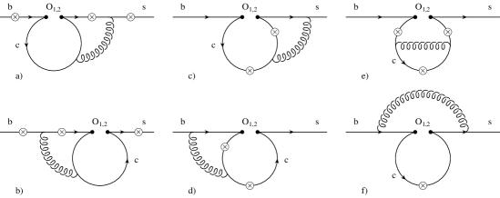
Figure 3.4: Complete list of two-loop Feynman diagrams for $b\rightarrow s\gamma^{*}$ associated with the operators $O_{1}$ and $O_{2}$. The fermions ($b$, $s$ and $c$ quarks) are represented by solid lines; the curly lines represent gluons. The circle-crosses denote the possible locations for emission of a virtual photon.

The 2-loop matrix elements of penguin operators have not yet been computed and will hence be neglected. Due to the small Wilson coefficients of the penguin operators, this should be a very good approximation. The matrix element of the chromomagnetic dipole operator [Figure (3.3-c)] is also given in [22] in expanded form. The exact result is given in Appendix B.3. All this combined, we obtain

$$C_{F}C^{(\rm nf)}_{\perp} = -\,\overline{C}_{2}F_{2}^{(7)}-C_{8}^{\rm eff}F_{8}^{(7)}$$ (3.65)

$$-\,\frac{s}{2m_{b}m_{B}}\left[\overline{C}_{2}F_{2}^{(9)}+2\overline{C}_{1}\left(F_{1}^{(9)}+\frac{1}{6}\,F_{2}^{(9)}\right)+C_{8}^{\rm eff}F_{8}^{(9)}\right],$$

$$C_{F}C^{(\rm nf)}_{\parallel} = \overline{C}_{2}F_{2}^{(7)}+C_{8}^{\rm eff}F_{8}^{(7)}$$ (3.66)

$$+\,\frac{m_{B}}{2m_{b}}\left[\overline{C}_{2}F_{2}^{(9)}+2\overline{C}_{1}\left(F_{1}^{(9)}+\frac{1}{6}\,F_{2}^{(9)}\right)+C_{8}^{\rm eff}F_{8}^{(9)}\right].$$

The quantities $F_{1,2}^{(7,9)}$ and $F_{8}^{(7,9)}$ are given in Appendix B.3, or can also be extracted from [22] in expanded form. In expressing the result in terms of the coefficients $\overline{C}_{1,2}$, we have made use of $F_{1}^{(7)}+F_{2}^{(7)}/6=0$. We also substituted $C_{8}$ by $C_{8}^{\rm eff}$, taking into account a subset of penguin contributions.

3.2.3 form factors values

$$\begin{array}[]{|l|llll|lll|}\hline\cr\hline\cr&A_{1}&A_{2}&A_{0}&V&T_{1}&T_{2}&T_{3}\\ \hline\cr F(0)&0.294&0.246&0.412&0.399&0.334&0.334&0.234\\ c_{1}&0.656&1.237&1.543&1.537&1.575&0.562&1.230\\ c_{2}&0.456&0.822&0.954&1.123&1.140&0.481&1.089\\ \hline\cr\hline\cr\end{array}$$

Table 3.2: Input values for the parameterization (3.70) of the $B\rightarrow K^{*}$ form factors. Renormalization scale for the penguin form factors $T_{i}$ is $\mu=m_{b}$ [31].

In the description of exclusive $B$-decays hadronic matrix elements $<X|{\cal O}_{i}|B>$ are involved. However, in order for these quantities to become available, it is necessary to confront the fact these hadrons are color bound state objects. While understood in principle, the non-perturbative nature of these bound states makes problematic the extraction of precision information about the exclusive $B$-physics. To explore them one faces a daunting theoretical challenge to evaluate first the corresponding form factors.

This is not a problem which has been solved in its entirely, nor is it likely ever to be. Rather, what is available is a variety of theoretical approaches and techniques, appropriate to a variety of specific problems and with varying levels of reliability. While approaches which are based directly on QCD, and which allow for quantitative error estimates, are clearly to be preferred, more model-dependent methods are often all that are available and thus have an important role to play as well.

Concerning our guess on the corresponding $B\rightarrow K^{*}$ form factors (see Eqs. (3.28) and (3.2)) we have combined roughly two theoretical approaches to compute them:

• First we have used the LEET symmetry to reduce the number of independent form factors from seven to two universal ones, namely $\xi^{(K^{*})}_{\perp}(s)$ and $\xi^{(K^{*})}_{||}(s)$ (see Eqs. (2.61)-(2.67)).

• At large recoil, namely $s=0$, the normalization of the LEET form factor $\xi_{\perp}^{(K^{*})}(0)$ is determined using the $B\rightarrow K^{*}\gamma$ experimental constraint on the corresponding NLO-LEET estimates. Thus, the magnetic moment form factors turns out to be in the range[?–?]

  $$T_{1}^{(K^{*})}(0)=0.28\pm 0.04.$$ (3.67)

  Thus, from Eqs. (3.67) and (2.65), the numerical value for the $\xi_{\perp}^{(K^{*})}$ at large recoil momentum is defined as

  $$\xi_{\perp}^{(K^{*})}(0)=0.28\pm 0.04.$$ (3.68)

• The second universal LEET form factor $\xi_{||}^{(K^{*})}(s)$ has to be modeled entirely from some approximate methods. For that we have used a non-perturbative approach, the so-called Light-cone sum-rule approach [86, 87], based on the approximate conformal invariance of QCD. While in principle this technique is rigorous, it suffers in its current practical implementations from a degree of uncontrolled model dependence (for a review see [90] and reference therein). Using the result of [30] for $B\rightarrow K^{*}$ form factors, presented in Table 3.2, which include NLO radiative corrections and higher twist corrections up to twist four. The result turns out to be:

  $$\xi_{||}^{K^{*}}(0)=0.31\pm 0.04.$$ (3.69)

• To extrapolate these form factors, namely $\xi_{\perp,||}^{(K^{*})}$, at small recoil (large values of $s$), we use the following parametrization (with its coefficients listed in Table 3.2):

  $$F(\hat{s})=F(0)\exp(c_{1}\hat{s}+c_{2}\hat{s}^{2}).$$ (3.70)

Using the ingredients described above, we show in Fig. 3.5 the corresponding LEET form factors $\xi^{(K^{*})}_{\perp}(s)$ and $\xi^{(K^{*})}_{||}(s)$. Note that the values used by Beneke el al. in ref.[25] are very different of the ones used by us. This descripency is related to the fact that their choice is based on the QCD sum rules estimates for $\xi^{(K^{*})}_{\perp}=0.35\pm 0.07$ and $\xi^{(K^{*})}_{||}=0.49\pm 0.09$. On the other hand, our values are somewhat lower than the corresponding estimates in the lattice-QCD framework, yielding [91] $T_{1}^{K^{*}}(0)=0.32^{+0.04}_{-0.02}$, and in the light cone QCD sum rule approach, which give typically $T_{1}^{K^{*}}(0)=0.38\pm 0.05$ [31]. (Earlier lattice-QCD results on $B\rightarrow K^{*}\gamma$ form factors are reviewed in [92].).

Finally, we have to keep in mind that such a descripency reflect after all our poor knowledge of this part of QCD, namely the non-perturbative QCD. Consequently, we can anticipate the fact that the long distance uncertainty in our analysis will be the dominant one.

\psfrag{a}{\hskip 0.0pt$\mathrm{s\ (GeV^{2})}$}\psfrag{c}{\hskip-28.45274pt$\xi^{(K^{*})}_{||}(s)$}\psfrag{b}{\hskip-28.45274pt$\xi^{(K^{*})}_{\perp}(s)$}\psfrag{d}{\hskip 0.0pt[AS]}\psfrag{e}{\hskip 0.0pt[BFS]}\includegraphics[width=512.1496pt,height=455.24408pt]{fig1.eps}

Figure 3.5: LEET form factors $\xi^{(K^{*})}_{{\perp},||}(s)$ for $B\rightarrow K^{*}\ l^{+}\ l^{-}$. The two columns denoted by [AS] and [BFS] represent, respectively, our $\xi^{(K^{*})}_{{\perp},||}(s)$ and the ones used by Beneke et al. in ref[25]. The central values are represented by the dashed curves, while the bands reflect the uncertainties on the form factors [28].

3.3 Decay Distributions in $B\rightarrow\ K^{*}\ell^{+}\ell^{-}$

Using all the machinery presented until this point we are able now to do the corresponding analysis for specific transitions. In this section, we present our Helicty analysis of the $B\rightarrow\ K^{*}\ell^{+}\ell^{-}$ decay. In the LEET Limit, the helicity amplitudes (3.26) are expressed as:

$$H^{L/R}_{+}(s) = {i\over\ {2\ m_{b}\ m_{B}\ (m_{B}+m_{K^{*}})\sqrt{s}}}\Big{[}-4\ {\cal T}_{1}(s)\ m_{b}\ (m_{B}-m_{K^{*}})\ (m_{B}+m_{K^{*}})^{2}\ E_{K^{*}}$$ (3.71)

$$+(\pm C_{10}-C_{9})\ m_{B}\ (m_{B}+m_{K^{*}})^{2}\ s\ A_{1}(s)$$

$$+2m_{B}\sqrt{\lambda}\Big{\{}2{\cal T}_{1}(s)\ m_{b}\ (m_{B}+m_{K^{*}})+(\mp C_{10}+C_{9})\ s\ V(s)\}\Big{\}}\Big{]},$$

$$H^{L/R}_{-}(s) = {i\over\ {2\ m_{b}\ m_{B}\ (m_{B}+m_{K^{*}})}\sqrt{s}}\Big{[}-4\ {\cal T}_{1}(s)\ m_{b}\ (m_{B}-m_{K^{*}})\ (m_{B}+m_{K^{*}})^{2}\ E_{K^{*}}$$ (3.72)

$$+(\pm C_{10}-C_{9})m_{B}(m_{B}+m_{K^{*}})^{2}\ s\ A_{1}(s)$$

$$-2m_{B}\sqrt{\lambda}\Big{\{}2{\cal T}_{1}(s)\ m_{b}(m_{B}+m_{K^{*}})+(\mp C_{10}+C_{9})sV(s)\}\Big{\}}\Big{]},$$

$$H^{L/R}_{0}(s) = {i\over{4\ m_{b}\ m_{B}\ m_{K^{*}}(-m_{B}^{2}+m_{K^{*}}^{2})s}}\Big{[}8\ \lambda\ m_{b}\ {\cal T}_{1}(s)\Big{\{}2(m_{B}^{2}-m_{K^{*}}^{2})E_{K^{*}}+m_{B}\ s\Big{\}}$$ (3.73)

$$+4\ \lambda\ m_{B}\ s\Big{\{}2\ m_{b}\ ({\cal T}_{3}(s)-\frac{m_{B}}{2\ E_{K^{*}}}\,{\cal T}_{2}(s))-A_{2}(s)(\pm C_{10}-C_{9})(m_{B}-m_{K^{*}})\Big{\}}$$

$$+(m_{B}-m_{K^{*}})(m_{B}+m_{K^{*}})^{2}(m_{B}^{2}-m_{K^{*}}^{2}-s)\Big{\{}4\ {\cal T}_{1}(s)\ m_{b}\ E_{K^{*}}(-m_{B}+m_{K^{*}})$$

$$+s\ m_{B}\ A_{1}(s)(\pm C_{10}-C_{9})\Big{\}}\Big{]}.$$

It is interesting to observe that in the Large Energy Effective Theory (LEET), both helicity amplitudes $|H_{+}^{L,R}(s)|^{2}$ and $|H_{-}^{L,R}(s)|^{2}$ have essentially one dependence on the universal form factor $\xi_{\perp}^{(K^{*})}$. However the helicity amplitude $|H_{0}^{L,R}(s)|^{2}$ is more model-dependent, since it depends on the two form factors $\xi_{\perp}^{(K^{*})}$ and $\xi_{||}^{(K^{*})}$.

In Figs. (3.7) and (3.7) we show respectively the helicity amplitudes $|H_{+,-}^{L}(s)|^{2}$ and $|H_{+,-}^{R}(s)|^{2}$ at leading and at next-to-leading order. We remark that both helicity amplitudes $|H_{+,-}^{R}(s)|^{2}$ are completely negligeable comparing to their left-helicity components. Moreover, the impact of the NLO corrections on the the amplitudes $|H_{+,-}^{L}(s)|^{2}$ and $|H_{+,-}^{R}(s)|^{2}$ increase considerably their magnitude up to $\sim 100\%$ in the small lepton invariant mass ($s<2~{}\textrm{GeV}^{2}$). The NLO uncertaities are dominated mainly by the $B$-meson light-cone distribution amplitudes $\lambda_{B,+}$, the $B$-decay constant $f_{B}$ and the form factor $\xi_{\perp}^{(K^{*})}$. The corresponding errors were calculated by varing mainly these parameters in the indicated range, one at a time, and adding the individual arrors in quadrature.

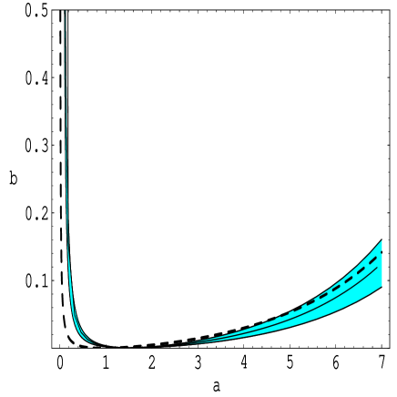
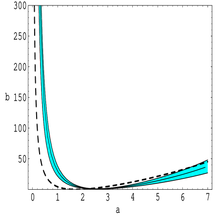
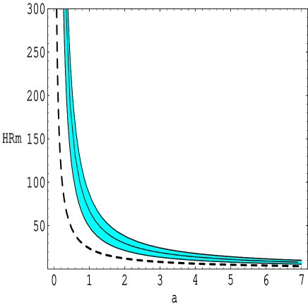
Figure 3.6: The helicity amplitude $|H_{+}^{L}(s)|^{2}$ (left-hand plot) and $|H_{-}^{L}(s)|^{2}$ (right-hand plot) at NLO (solid center line) and LO (dashed). The band reflects theoretical uncertainties from the input parameters [28].

Figure 3.7: The helicity amplitude $|H_{+}^{R}(s)|^{2}$ (left-hand plot) and $|H_{-}^{R}(s)|^{2}$ (right-hand plot) at NLO (solid center line) and LO (dashed). The band reflects theoretical uncertainties from the input parameters [28].

Using the above helicity amplitudes and taking the narrow resonance limit of $K^{*}$ meson, i.e., using the equations

$$\Gamma_{K^{*}}=\frac{g_{K^{*}K\pi}^{2}m_{K^{*}}}{48\pi}~{},$$

$$\lim_{\Gamma_{K^{*}}\rightarrow 0}\frac{\Gamma_{K^{*}}m_{K^{*}}}{(p^{2}-m_{K^{*}}^{2})^{2}+m_{K^{*}}^{2}\Gamma_{K^{*}}^{2}}=\pi\delta(p^{2}-m_{K^{*}}^{2})~{},$$ (3.74)

we can perform the integration over $p^{2}$ in Eq. (3.27) and obtain the fourth differential angular distribution of $B\rightarrow K^{*}(\rightarrow K\pi)\ \ell^{+}\ell^{-}$with respect to dilepton mass squared $s$, the azimuthal angle $\phi$, the polar angles $\theta_{K}$ and $\theta_{+}$,

$${d^{4}\Gamma\over ds\ d\cos\theta_{K}\ d\cos\theta_{+}\ d\phi}={3\ \alpha_{em}^{2}G_{F}^{2}\sqrt{\lambda}m_{b}^{2}|V_{tb}V_{ts}^{*}|^{2}\over 128(2\pi)^{6}m_{B}^{3}}$$ (3.75)

$$\times\Big{\{}4\ cos^{2}\theta_{K}\ sin^{2}\theta_{+}\ \Big{(}|H^{R}_{0}(s)|^{2}+|H^{L}_{0}(s)|^{2}\Big{)}$$

$$+sin^{2}\theta_{K}\ (1+cos^{2}\theta_{+})\ \Big{(}|H^{L}_{+}(s)|^{2}+|H^{L}_{-}(s)|^{2}+|H^{R}_{+}(s)|^{2}+|H^{R}_{-}(s)|^{2}\Big{)}$$

$$-2\ sin^{2}\theta_{K}\ sin^{2}\theta_{+}\ \Big{[}\ cos2\phi\ Re\Big{(}H^{R}_{+}(s)H^{R*}_{-}(s)+H^{L}_{+}(s)H^{L*}_{-}(s)\Big{)}$$

$$-sin2\phi\ Im\Big{(}H^{R}_{+}(s)H^{R*}_{-}(s)+H^{L}_{+}(s)H^{L*}_{-}(s)\Big{)}\ \Big{]}$$

$$-sin2\theta_{K}\ sin2\theta_{+}\ \Big{[}\ cos\phi\ Re\Big{(}H^{R}_{+}(s)H^{R*}_{0}(s)+H^{R}_{-}(s)H^{R*}_{0}(s)+H^{L}_{+}(s)H^{L*}_{0}(s)+H^{L}_{-}(s)H^{L*}_{0}(s)\Big{)}$$

$$-sin\phi\ Im\Big{(}H^{R}_{+}(s)H^{R*}_{0}(s)-H^{R}_{-}(s)H^{R*}_{0}(s)+H^{L}_{+}(s)H^{L*}_{0}(s)-H^{L}_{-}(s)H^{L*}_{0}(s)\Big{)}\ \Big{]}$$

$$-2\ sin^{2}\theta_{K}\ cos\theta_{+}\ \Big{(}|H^{R}_{+}(s)|^{2}-|H^{R}_{-}(s)|^{2}-|H^{L}_{+}(s)|^{2}+|H^{L}_{-}(s)|^{2}\Big{)}$$

$$+2\ sin\theta_{+}\ sin2\theta_{K}\ \Big{[}\ cos\phi\ Re\Big{(}H^{R}_{+}(s)H^{R*}_{0}(s)-H^{R}_{-}(s)H^{R*}_{0}(s)-H^{L}_{+}(s)H^{L*}_{0}(s)+H^{L}_{-}(s)H^{L*}_{0}(s)\Big{)}$$

$$-sin\phi\ Im\Big{(}H^{R}_{+}(s)H^{R*}_{0}(s)+H^{R}_{-}(s)H^{R*}_{0}(s)-H^{L}_{+}(s)H^{L*}_{0}(s)-H^{L}_{-}(s)H^{L*}_{0}(s)\Big{)}\Big{]}\Big{\}}.$$

3.3.1 Dalitz distributions

If we integrate out the angle $\theta_{K}$ and $\theta_{+}$ from Eq.(3.75), we get the double $\phi$ angular distribution:

$${d^{2}{\cal B}\over d\phi\ ds}=\tau_{B}{\alpha_{em}^{2}G_{F}^{2}\over 384\pi^{5}}\sqrt{\lambda}{m_{b}^{2}\over m_{B}^{3}}|V_{tb}V_{ts}^{*}|^{2}\ {1\over 2\pi}\ \Big{\{}|H_{0}(s)|^{2}+|H_{+}(s)|^{2}+|H_{-}(s)|^{2}$$ (3.76)

$$-cos2\phi\ Re\Big{(}H_{+}^{R}(s)H_{-}^{R*}(s)+H_{+}^{L}(s)H_{-}^{L*}(s)\Big{)}+sin2\phi\ Im\Big{(}H_{+}^{R}(s)H_{-}^{R*}(s)+H_{+}^{L}(s)H_{-}^{L*}(s)\Big{)}\Big{\}},$$

where $\tau_{B}$ is the life time of the $B$-meson, and the various terms in the expansion above can be specified , as follows :

$$|H_{0}(s)|^{2} = |H^{L}_{0}(s)|^{2}+|H^{R}_{0}(s)|^{2},$$

$$|H_{+}(s)|^{2} = |H^{L}_{+}(s)|^{2}+|H^{R}_{+}(s)|^{2},$$

$$|H_{-}(s)|^{2} = |H^{L}_{-}(s)|^{2}+|H^{R}_{-}(s)|^{2}.$$ (3.77)

\psfrag{c}{\hskip 8.5359pt$s\ (\textrm{GeV}^{2})$}\psfrag{a}{\hskip-85.35826pt\Large{${d^{2}{\cal B}\over ds\ d\cos\theta_{+}\ 10^{-8}}$}}\psfrag{b}{$\textrm{cos}\theta_{+}$}\includegraphics[width=341.43306pt,height=256.0748pt]{fig6.eps}

Figure 3.8: Dalitz distribution ${d^{2}{\cal B}\over d\cos\theta_{+}\ ds}$ for $B\rightarrow K^{*}\ \ell^{+}\ \ell^{-}$ [28] .

Similarly, we can get respectively the $\theta_{K}$ and $\theta_{+}$ angular distributions as following:

$${d^{2}{\cal B}\over d\cos\theta_{K}\ ds} = \tau_{B}{\alpha_{em}^{2}G_{F}^{2}\over 384\pi^{5}}\sqrt{\lambda}{m_{b}^{2}\over m_{B}^{3}}|V_{tb}V_{ts}^{*}|^{2}\ {3\over 4}\ \Big{\{}2\ cos^{2}\theta_{K}\ |H_{0}(s)|^{2}$$ (3.79)

$$+sin^{2}\theta_{K}\ \Big{(}|H_{+}(s)|^{2}+|H_{-}(s)|^{2}\Big{)}\Big{\}},$$

and

$${d^{2}{\cal B}\over d\cos\theta_{+}\ ds} = \tau_{B}{\alpha_{em}^{2}G_{F}^{2}\over 384\pi^{5}}\sqrt{\lambda}{m_{b}^{2}\over m_{B}^{3}}|V_{tb}V_{ts}^{*}|^{2}\ {3\over 8}\ \Big{\{}2\ sin^{2}\theta_{+}\ |H_{0}(s)|^{2}$$ (3.81)

$$+(1+cos\theta_{+})^{2}\ |H_{+}^{L}(s)|^{2}+(1-cos\theta_{+})^{2}\ |H_{+}^{R}(s)|^{2}$$

$$+(1-cos\theta_{+})^{2}\ |H_{-}^{L}(s)|^{2}+(1+cos\theta_{+})^{2}\ |H_{-}^{R}(s)|^{2}\Big{\}},$$

$$={d^{2}{\cal B}_{|H_{0}|^{2}}\over d\cos\theta_{+}\ ds}+{d^{2}{\cal B}_{|H_{-}|^{2}}\over d\cos\theta_{+}\ ds}+{d^{2}{\cal B}_{|H_{+}|^{2}}\over d\cos\theta_{+}\displaystyle},$$

where the various terms in Eq. (3.81), namely $d^{2}{\cal B}_{|H_{0}|^{2}}/d\cos\theta_{+}\ ds$, $d^{2}{\cal B}_{|H_{-}|^{2}}/d\cos\theta_{+}\ ds$ and $d^{2}{\cal B}_{|H_{+}|^{2}}/d\cos\theta_{+}\ ds$ can be defined respectively,as follows:

$${d^{2}{\cal B}_{|H_{0}|^{2}}\over d\cos\theta_{+}\ ds} = \tau_{B}{\alpha_{em}^{2}G_{F}^{2}\over 384\pi^{5}}\sqrt{\lambda}{m_{b}^{2}\over m_{B}^{3}}|V_{tb}V_{ts}^{*}|^{2}\ {3\over 8}\ \Big{\{}2\ sin^{2}\theta_{+}\ |H_{0}(s)|^{2}\Big{\}},$$ (3.82)

$${d^{2}{\cal B}_{|H_{-}|^{2}}\over d\cos\theta_{+}\ ds} = \tau_{B}{\alpha_{em}^{2}G_{F}^{2}\over 384\pi^{5}}\sqrt{\lambda}{m_{b}^{2}\over m_{B}^{3}}|V_{tb}V_{ts}^{*}|^{2}\ {3\over 8}\ \Big{\{}(1-cos\theta_{+})^{2}\ |H_{-}^{L}(s)|^{2}+(1+cos\theta_{+})^{2}\ |H_{-}^{R}(s)|^{2}\Big{\}},$$

$${d^{2}{\cal B}_{|H_{+}|^{2}}\over d\cos\theta_{+}\ ds} = \tau_{B}{\alpha_{em}^{2}G_{F}^{2}\over 384\pi^{5}}\sqrt{\lambda}{m_{b}^{2}\over m_{B}^{3}}|V_{tb}V_{ts}^{*}|^{2}\ {3\over 8}\ \Big{\{}(1+cos\theta_{+})^{2}\ |H_{+}^{L}(s)|^{2}+(1-cos\theta_{+})^{2}\ |H_{+}^{R}(s)|^{2}\Big{\}}.$$

\psfrag{c}{\hskip 8.5359pt$s\ (\textrm{GeV}^{2})$}\psfrag{b}{$\textrm{cos}\theta_{+}$}\psfrag{a}{\hskip-85.35826pt\Large{${d^{2}{\cal B}_{|H_{-}|^{2}}\over ds\ d\cos\theta_{+}\ 10^{-8}}$}}\includegraphics[width=341.43306pt,height=256.0748pt]{fig7.eps}

Figure 3.9: Partial Dalitz distribution ${d^{2}{\cal B}_{|H_{-}|^{2}}\over d\cos\theta_{+}\ ds}$ for $B\rightarrow K^{*}\ \ell^{+}\ \ell^{-}$ [28] .

\psfrag{c}{\hskip 8.5359pt$s\ (\textrm{GeV}^{2})$}\psfrag{b}{$\textrm{cos}\theta_{+}$}\psfrag{a}{\hskip-85.35826pt\Large{${d^{2}{\cal B}_{|H_{-}|^{2}}\over ds\ d\cos\theta_{+}\ 10^{-8}}$}}\psfrag{a}{\hskip-85.35826pt\Large{${d^{2}{\cal B}_{|H_{0}|^{2}}\over ds\ d\cos\theta_{+}\ 10^{-8}}$}}\includegraphics[width=341.43306pt,height=256.0748pt]{fig8.eps}

Figure 3.10: Partial Dalitz distribution ${d^{2}{\cal B}_{|H_{0}|^{2}}\over d\cos\theta_{+}\ ds}$ for $B\rightarrow K^{*}\ell^{+}\ell^{-}$ [28] .

Note that the polar angle distribution functions in Eqs. (3.79), (3.81) and (3.82) depend only on the modular square terms of the helicity amplitudes, which give the decay width of the semileptonic decay (see next section).

Using our central input parameters given in Tables (3.1) and (A.1) (see Apendix  A.1), we show in Figs. (3.8), (3.10) and (3.10) at the NLO accuracy the total Dalitz distribution $d^{2}{\cal B}/d\cos\theta_{+}\ ds$, the two angular partial distributions $d^{2}{\cal B}_{|H_{-}|^{2}}/d\cos\theta_{+}\ ds$ and $d^{2}{\cal B}_{|H_{0}|^{2}}/d\cos\theta_{+}\ ds$, respectively. From the experimental point of view these Dalitz distribution can serve as a double check of whether the branching fraction is different from the SM predictions.

3.3.2 Dilepton mass spectrum and Forward-backward asymmetry

Finally, after integrating over the polar angles $\phi$, $\theta_{+}$ and $\theta_{K}$, we derive the total differential branching ratio in the scaled dilepton invariant mass for $B\rightarrow K^{*}\ell^{+}\ell^{-}$,

$${d{\cal B}\over ds} = \tau_{B}{\alpha_{em}^{2}G_{F}^{2}\over 384\pi^{5}}\sqrt{\lambda}{m_{b}^{2}\over m_{B}^{3}}|V_{tb}V_{ts}^{*}|^{2}\Big{\{}|H_{+}(s)|^{2}+|H_{-}(s)|^{2}+|H_{0}(s)|^{2}\Big{\}}$$ (3.83)

$$= {d{\cal B}_{|H_{+}|^{2}}\over ds}+{d{\cal B}_{|H_{-}|^{2}}\over ds}+{d{\cal B}_{|H_{0}|^{2}}\over ds},$$ (3.84)

where the various terms in the Eq. (3.83), read as

$${d{\cal B}_{|H_{+}|^{2}}\over ds} = \tau_{B}{\alpha_{em}^{2}G_{F}^{2}\over 384\pi^{5}}\sqrt{\lambda}{m_{b}^{2}\over m_{B}^{3}}|V_{tb}V_{ts}^{*}|^{2}\,\,|H_{+}(s)|^{2},$$ (3.85)

$${d{\cal B}_{|H_{-}|^{2}}\over ds} = \tau_{B}{\alpha_{em}^{2}G_{F}^{2}\over 384\pi^{5}}\sqrt{\lambda}{m_{b}^{2}\over m_{B}^{3}}|V_{tb}V_{ts}^{*}|^{2}\,\,|H_{-}(s)|^{2},$$ (3.86)

$${d{\cal B}_{|H_{0}|^{2}}\over ds} = \tau_{B}{\alpha_{em}^{2}G_{F}^{2}\over 384\pi^{5}}\sqrt{\lambda}{m_{b}^{2}\over m_{B}^{3}}|V_{tb}V_{ts}^{*}|^{2}\,\,|H_{0}(s)|^{2}.$$ (3.87)

The partial lepton invariant mass spectrum $d{\cal B}_{|H_{-}|^{2}}/ds$, $d{\cal B}_{|H_{+}|^{2}}/ds$ and $d{\cal B}_{|H_{0}|^{2}}/ds$ are shown in Fig. (3.11) showing in each case the next-to-leading order and leading order results. We remark that the partial single distribution $d{\cal B}_{|H_{+}|^{2}}/ds$ is completely negligeable comparing to the others. In fact this is due to the smallness of the helicity amplitude $|H_{+}|^{2}$, as it is shown in Figs. (3.7) and (3.7).

In Fig. (3.12), we plot the total dilepton invariant mass $d{\cal B}/ds$ at next-to-leading order and leading order. As it is shown in Figs. (3.11–upper plot) and (3.12) the total decay rate is dominated by the contribution of the helicity $|H_{-}|$ component.

We Note that the next-to-leading order correction to the lepton invariant mass spectrum in $B\rightarrow K^{*}\ell^{+}\ell^{-}$ is significant in the low dilepton mass region $(s\leq 2~{}\textrm{GeV}^{2})$ but small beyond that shown for the anticipated validity of the LEET theory $(s\leq 8~{}\textrm{GeV}^{2})$. Apparently rather large uncertainty of our prediction is mainly due to the form factors with their current large uncertainty and to a lesser extent respectively due to $\lambda_{B,+}^{-1}$ and the $B$-decay constant.

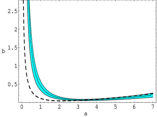
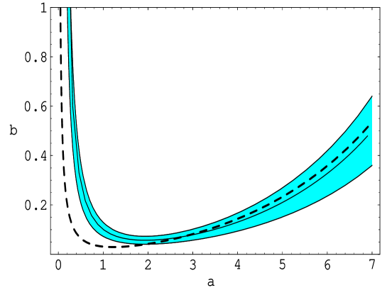
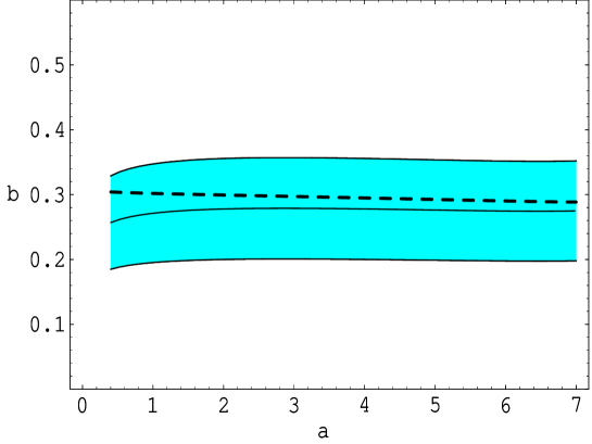
Figure 3.11: The dilepton invariant mass distributions ${d{\cal B}_{|H_{-}|^{2}}\over ds}$ (upper-plot), ${dBr_{|H_{+}|^{2}}\over ds}$ (middle-plot) and ${d{\cal B}_{|H_{0}|^{2}}\over ds}$ (lower-plot) for $B\rightarrow K^{*}\ell^{+}\ell^{-}$ at NLO (solid center line) and LO (dashed).The band reflects the theoretical uncertainties from input parameters [28, 29].

\psfrag{a}{\hskip 0.0pt$\mathrm{s\ (GeV^{2})}$}\psfrag{b}{\hskip-71.13188pt\Large{${d{\cal B}\over ds\ 10^{-7}}$}}\psfrag{c}{}\includegraphics[width=398.33858pt,height=284.52756pt]{fig12.eps}

Figure 3.12: The total dilepton invariant mass distribution for $B\rightarrow K^{*}\ell^{+}\ell^{-}$ at NLO (solid center line) and LO (dashed). The band reflects theoretical uncertainties from the input parameters [28].

Besides the differential branching ratio, $B\rightarrow K^{*}\ell^{+}\ell^{-}$ decay offers other distributions (with different combinations of Wilson coefficients) to be measured. An interesting quantity is the Forward-Backward (FB) asymmetry defined in [19, 49]

$$\frac{{\rm d}{\cal A}_{\rm FB}}{{\rm d}\hat{s}}=-\int_{0}^{{\hat{u}}(\hat{s})}{\rm d}{\hat{u}}\frac{{\rm d}^{2}\Gamma}{{\rm d}{\hat{u}}\,{\rm d}\hat{s}}+\int_{-{\hat{u}}(\hat{s})}^{0}{\rm d}{\hat{u}}\frac{{\rm d}^{2}\Gamma}{{\rm d}{\hat{u}}\,{\rm d}\hat{s}}\;,$$ (3.88)

where the variable $\hat{u}$ corresponds to $\theta_{+}$, the angle between the momentum of the $B$-meson and the positively charged lepton $\ell^{+}$ in the dilepton CMS frame, through the relation $\hat{u}=-\hat{u}(\hat{s})\cos\theta_{+}$, and bounded as

$$-\hat{u}(\hat{s})\leq\hat{u}\leq\hat{u}(\hat{s})\;,$$ (3.89)

with

$$\hat{u}(\hat{s})={2\over m_{B}^{2}}\sqrt{\lambda(1-4{\hat{m}_{\ell}^{2}\over\hat{s}})}.$$ (3.90)

\psfrag{a}{$s\ (GeV^{2})$}\psfrag{b}{\hskip-71.13188pt$dA_{FB}/ds$}\psfrag{c}{\hskip 0.0pt}\includegraphics[width=398.33858pt,height=284.52756pt]{figsm1.eps}

Figure 3.13: The forward-backward asymmetry in $B\rightarrow K^{*}\ell^{+}\ell^{-}$ decay at NLO (solid center line) and LO (dashed). The band reflects the theoretical uncertainties from the input parameters [28].

It is interesting to observe that at the leading order in the LEET approach, the FB-asymmetry in $B\rightarrow K^{*}\ell^{+}\ell^{-}$ decays depends on one universal form factor $\xi^{(K^{*})}_{\perp}(s)$, and reads as follows

$$\frac{{\rm d}{\cal A}_{\rm FB}}{{\rm d}\hat{s}} = \frac{G_{F}^{2}\,\alpha_{em}^{2}\,m_{B}^{5}}{2^{8}\pi^{5}}\left|V_{ts}^{\ast}V_{tb}\right|^{2}\,\hat{s}\,{\hat{u}}(\hat{s})^{2}$$

$$\times{C_{10}}\left[(-{C_{7}}^{\rm eff}){\hat{m}_{b}\over\ \hat{s}}(-1+\hat{m}_{K^{*}}^{2}+\hat{s})+2\ {E_{K^{*}}\over m_{B}}\Big{(}{C_{7}}^{\rm eff}\ {\hat{m}_{b}\over\ \hat{s}}+{\rm Re}[{C_{9}}^{\rm eff}]\Big{)}\right]\xi^{(K^{*})}_{\perp}(s)^{2}\;.$$

It has been noted in [93] that the location of the forward-backward asymmetry zero $\hat{s}_{0}$ is nearly independent of particular form factor models. An explanation of this fact was given in [31], where it has been noted that the form factor ratios on which the asymmetry zero depends are predicted free of hadronic uncertainties in the combined heavy quark and large energy limit. Thus the position of the zero $\hat{s}_{0}$ is given by

$${\rm Re}\Big{(}{C_{9}}^{\rm eff}(\hat{s}_{0})\Big{)}=-\frac{\hat{m}_{b}}{\hat{s}_{0}}{C_{7}}^{\rm eff}\left\{\frac{1-\hat{m}_{K^{*}}^{2}-\hat{s}}{1+\hat{m}_{K^{*}}^{2}-\hat{s}}+1\right\}\;,$$ (3.94)

which depends on the value of $m_{b}$ and the ratio of the effective coefficients ${C_{7}}^{\rm eff}/{\rm Re}\Big{(}{C_{9}}^{\rm eff}(\hat{s}_{0})\Big{)}$.

Thus, the precision on the zero-point of the FB-asymmetry in $B\rightarrow K^{*}\ell^{+}\ell^{-}$ is determined essentially by the precision of the ratio of the effective coefficients and $m_{b}$. We find the insensitivity of $\hat{s}_{0}$ to the decay form factors in $B\rightarrow K^{*}\ell^{+}\ell^{-}$ a remarkable result, which has also been discussed in [93]. However, the LEET-based result in Eq. (3.94) stands theoretically on more rigorous grounds than the arguments based on scanning a number of form factor models. Our result for FBA is shown in Fig. (3.13) to LO and NLO accuracy. With the coefficients given in Table (3.1) and $m_{b}=4.6$ GeV, we find the LO location of the FB-asymmetry zero is $s_{0}\simeq 3.4\,\mbox{GeV}^{2}$.

In [63] the effect of the (factorizable) radiative corrections to the form factor has been studied and has been found to shift the position of the asymmetry zero about 5% towards larger values. However the effect of both, factorizable and non-factorizable radiative corrections modify considerably the location of the FB-asymmetry zero $s_{0}$. As it is shown in Fig. (3.13), the numerical effect of NLO corrections amounts to a substantial enhancement of the FB asymmetry for intermediate lepton invariant mass ($s=1.5-6$ GeV²) and a significant shift of the location of the FB-asymmetry zero to $s_{0}\simeq 4.7\,\mbox{GeV}^{2}$. The dominant uncertainty (between $5\%$ and up $55\%$) is shared mainly between the $B$-meson light-cone distribution amplitudes $\lambda_{B,+}$, the $B$-decay constant $f_{B}$ and the form factor $\xi_{\perp}^{(K^{*})}$.

3.3.3 Transversity Amplitudes for $B\rightarrow K^{*}\ell^{+}\ell^{-}$

The decay $B\rightarrow J/\psi K^{*}$ is described by three amplitudes $({\cal A}_{i};i=0,\parallel,\perp)$ in the transversity basis, where ${\cal A}_{0}(s)$, ${\cal A}_{||}(s)$ and ${\cal A}_{\perp}(s)$ have CP eigenvalues $+1,+1$ and $-1$, respectively [?–?]. Here, ${\cal A}_{0}(s)$ corresponds to the longitudinal polarization of the vector meson $K^{*}$ and ${\cal A}_{||}(s)$ and ${\cal A}_{\perp}(s)$ correspond to parallel and transverse polarizations, respectively. The relative phase between the parallel (transverse) amplitude and the longitudinal amplitude is given by $\phi_{\parallel(\perp)}(s)\equiv\mbox{arg}\Big{(}{\cal A}_{\parallel(\perp)}/{\cal A}_{0}(s)\Big{)}$.

The transversity frame is defined as the $J/\psi$ rest frame (see Fig. (3.14)). The $K^{*}$ direction defines the negative $x$ axis. The $K\pi$ decay plane defines the $(x,y)$ plane, with $y$ oriented such that $p_{y}(K)>0$. The $z$ axis is the normal to this plane, and the coordinate system is right-handed. The transversity angles $\theta_{tr}$ and $\phi_{tr}$ are defined as the polar and azimuthal angles of the positively charged lepton from the $J/\psi$ decay; $\theta_{K^{*}}$ is the $K^{*}$ helicity angle defined in the $K^{*}$ rest frame as the angle between the $K$ direction and the direction opposite to the $J/\psi$. This basis has been used by the CLEO [32], CDF [33], BABAR [34], and the BELLE [35] collaborations to project out the amplitudes in the decay $B\rightarrow J/\psi K^{*}$ with well-defined CP eigenvalues in their measurements of the quantity $\sin 2\beta$, where $\beta$ is an inner angle of the unitarity triangle.

We also adopt this basis and analyze the various amplitudes from the non-resonant (equivalently short-distance) decay $B\rightarrow K^{*}\ell^{+}\ell^{-}$. In this basis, both the resonant $B\rightarrow K^{*}J/\psi\rightarrow K^{*}\ell^{+}\ell^{-}$ (already measured) and the non-resonant ($B\rightarrow K^{*}\ell^{+}\ell^{-}$) amplitudes turn out to be very similar, as we show here.

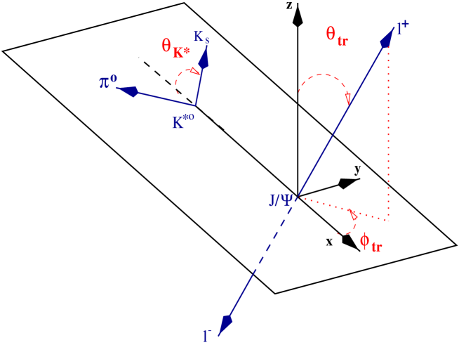
Figure 3.14: Definitions of the transversity angles $\theta_{tr}$, $\phi_{tr}$, and $\theta_{K^{*}}$. The angles $\theta_{tr}$ and $\phi_{tr}$ are determined in the $J/\psi$ rest frame. The angle $\theta_{K^{*}}$ is determined in the $K^{*}$ rest frame.

The angular distribution is given in terms of the linear polarization basis (${\cal A}_{\pm 1}(s)=({\cal A}_{\parallel}(s)\pm{\cal A}_{\perp}(s))/\sqrt{2}$) and ${\cal A}_{0}(s)$ by

$$\displaystyle\frac{d^{4}\Gamma}{ds\;\,d\cos{\theta_{tr}}\;\,d\cos{\theta_{K^{*}}}\;\,d\phi_{tr}} = f_{1}(w)\cdot|{\cal A}_{0}(s)|^{2}+f_{2}(w)\cdot|{\cal A}_{\parallel}(s)|^{2}+f_{3}(w)\cdot|{\cal A}_{\perp}(s)|^{2}$$

$$+ \eta f_{4}(w)\cdot{\rm Im}({\cal A}^{*}_{\parallel}(s){\cal A}_{\perp}(s))+f_{5}(w)\cdot{\rm Re}({\cal A}^{*}_{0}(s){\cal A}_{\parallel}(s))$$

$$+ \eta f_{6}(w)\cdot{\rm Im}({\cal A}^{*}_{0}(s){\cal A}_{\perp}(s))~{},$$

where $\eta=+1(-1)$ for $B^{0}$ and $B^{+}$ ($\overline{B}^{0}$ and $B^{-}$), and the coefficients $f_{i=1,...,6}$, which depend on the transversity angles $w=(\theta_{K^{*}},\theta_{tr},\phi_{tr})$, are given by:

$$f_{1}(w) = ~{}~{}\ \,9/(32\pi)\cdot\,2\cos^{2}{\theta_{K^{*}}}(1-\sin^{2}{\theta_{tr}}\cos^{2}{\phi_{tr}}),$$

$$f_{2}(w) = ~{}~{}\ \,9/(32\pi)\cdot\,\sin^{2}{\theta_{K^{*}}}(1-\sin^{2}{\theta_{tr}}\sin^{2}{\phi_{tr}}),$$

$$f_{3}(w) = ~{}~{}\ \,9/(32\pi)\cdot\,\sin^{2}{\theta_{K^{*}}}\sin^{2}{\theta_{tr}},$$

$$f_{4}(w) = ~{}~{}\ \,9/(32\pi)\cdot\,\sin^{2}{\theta_{K^{*}}}\sin{2\theta_{tr}}\sin{\phi_{tr}},$$

$$f_{5}(w) = -\ \,9/(32\pi)\cdot\,1/\sqrt{2}\cdot\sin{2\theta_{K^{*}}}\sin^{2}{\theta_{tr}}\sin{2\phi_{tr}},$$

$$f_{6}(w) = ~{}~{}\ \,9/(32\pi)\cdot\,1/\sqrt{2}\cdot\sin{2\theta_{K^{*}}}\sin{2\theta_{tr}}\cos{\phi_{tr}}~{}.$$

Group	$|\hat{\cal A}_{0}|^{2}$	$|\hat{\cal A}_{\perp}|^{2}$	$|\hat{\cal A}_{||}|^{2}$	$\phi_{\perp}$	$\phi_{\parallel}$
CLEO[32]	$0.52\pm 0.08$	$0.16\pm 0.09$	$0.32\pm 0.12$	$-3.03\pm 0.46$	$-3.00\pm 0.37$
CDF[33]	$0.59\pm 0.06$	$0.13^{+0.13}_{-0.11}$	$0.28\pm 0.12$	$-2.58\pm 0.54$	$-2.20\pm 0.47$
BaBar[34]	$0.60\pm 0.04$	$0.16\pm 0.03$	$0.24\pm 0.04$	$-2.97\pm 0.17$	$-2.50\pm 0.22$
Belle [35]	$0.60\pm 0.05$	$0.19\pm 0.06$	$0.21\pm 0.08$	$-3.15\pm 0.21$	$-2.86\pm 0.25$
AS [28]	$0.51$	$0.21$	$0.28$	$-3.25$	$-3.04$

Table 3.3: Current measurements of the decay amplitudes in the transversity basis for the decay $B\rightarrow J/\psi K^{*}$ . The corresponding amplitudes for the non-resonant decay $B\rightarrow K^{*}\ell^{+}\ell^{-}$ worked out in this paper in the LO approximation at $m_{\ell^{+}\ell^{-}}^{2}=m_{J/\psi}^{2}$ are given in the last row [28].

In terms of the helicity amplitudes $H^{L/R}_{\pm 1,0}$, introduced earlier, the amplitudes in the linear polarization basis, ${\cal A}_{0,\perp,\parallel}$, can be calculated from the relation:

$${\cal A}_{0}(s) = \kappa\Big{(}H^{L}_{0}(s)+H^{R}_{0}(s)\Big{)}~{},$$

$${\cal A}_{\pm 1}(s) = \kappa\Big{(}H^{L}_{\pm}(s)+H^{R}_{\pm}(s)\Big{)}~{},$$

with $\kappa^{2}={\alpha_{em}^{2}G_{F}^{2}\over 384\pi^{5}}\sqrt{\lambda}{m_{b}^{2}\over m_{B}^{3}}|V_{tb}V_{ts}^{*}|^{2}~{}$.

Experimental results are conventionally expressed in terms of the spin amplitudes $\hat{\cal A}_{0,\bot,\|}$ normalized to unity, with $|\hat{\cal A}_{0}|^{2}+|\hat{\cal A}_{\bot}|^{2}+|\hat{\cal A}_{\|}|^{2}=1$. We show the polarization fractions, $\Gamma_{0}/\Gamma=|\hat{\cal A}_{0}(s)|^{2}$, $\Gamma_{\parallel}/\Gamma=|\hat{\cal A}_{\parallel}(s)|^{2}$ and $\Gamma_{\perp}/\Gamma=|\hat{\cal A}_{\perp}(s)|^{2}$ in the leading and next-to-leading order for the decay $B\rightarrow K^{*}\ell^{+}\ell^{-}$ in Fig. (3.15), respectively. Since the interference terms in the angular distribution are limited to Re(${\cal A}_{||}{\cal A}_{0}^{*}$), Im(${\cal A}_{\perp}{\cal A}_{0}^{*}$) and Im(${\cal A}_{\perp}{\cal A}_{||}^{*}$), there exists a phase ambiguity:

$$\phi_{||} \rightarrow -\phi_{||}~{},$$ (3.95)

$$\phi_{\perp} \rightarrow \pm\pi-\phi_{\perp}~{},$$ (3.96)

$$\phi_{\perp}-\phi_{||} \rightarrow \pm\pi-(\phi_{\perp}-\phi_{||})~{}.$$ (3.97)

To avoid this, we have plotted in Fig. (3.16) the functions $\cos\phi_{\parallel,\perp}(s)$ and $\sin\phi_{\parallel,\perp}(s)$, showing their behaviour at the leading and next-to-leading order. The dashed lines in these figures correspond to using the LO amplitudes, calculated in the LEET approach. In this order, the bulk of the parametric uncertainty resulting from the form factors cancels. Although, strictly speaking, the domain of validity of the LEET-based distributions is limited by the requirement of large energy of the $K^{*}$ (which we have translated into approximately $s<8~{}\mbox{GeV}^{2}$), we show this distribution for the entire $s$-region allowed kinematically in $B\rightarrow K^{*}\ell^{+}\ell^{-}$. The shaded curves correspond to using the NLO contributions in the LEET approach.

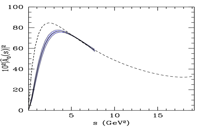
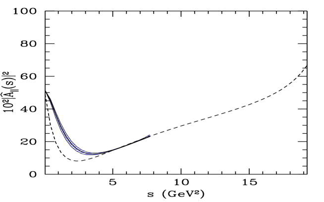
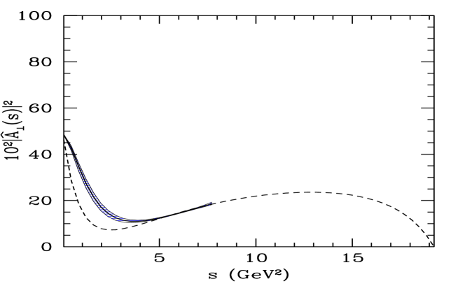
Figure 3.15: The helicity amplitudes $|\hat{\cal A}_{0}(s)|^{2}$ (upper-plot), $|\hat{\cal A}_{\parallel}(s)|^{2}$ (middle-plot) and $|\hat{\cal A}_{\perp}(s)|^{2}$ (lower-plot) in $B\rightarrow K^{*}\ell^{+}\ell^{-}$ at NLO (solid center line) and LO (dashed). The band for NLO reflects theoretical uncertainties from input parameters [28].

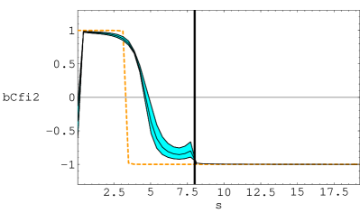
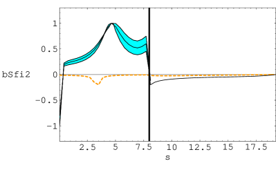
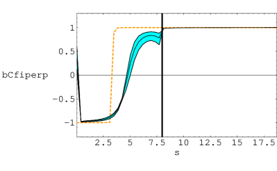
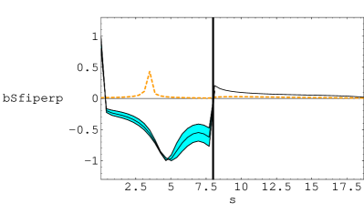
Figure 3.16: The functions $\cos\phi_{||,\perp}(s)$ and $\sin\phi_{||,\perp}(s)$ at NLO (solid center line) and LO (dashed). The band reflects all theoretical uncertainties from parameters with most of the uncertainty due to the form factors $\xi^{(K^{*})}_{i}(0)$.The vertical line at s = 8 $\mbox{GeV}^{2}$ represents the domain of validity of the LEET approach in our case [28].

We compare the resulting amplitudes $|\hat{\cal A}_{0}|^{2}$, $|\hat{\cal A}_{\perp}|^{2}$, $|\hat{\cal A}_{\parallel}|^{2}$, $\phi_{\parallel}(s)$, and $\phi_{\perp}(s)$ at the value $s=m_{J/\psi}^{2}$ with the corresponding results from the four experiments in Table (3.3). In comparing these results for the phases, we had to make a choice between the two phase conventions shown in Eq. (3.97) and the phases shown in the last row of this table correspond to adopting the lower signs in these equations. We note that the short-distance amplitudes from the decay $B\rightarrow K^{*}\ell^{+}\ell^{-}$ are similar to their resonant counterparts measured in the decay $B\rightarrow J/\psi K^{*}$. We also note that a helicity analysis of the decay $B\rightarrow J/\psi K^{*}$ has been performed in the QCD factorization approach by Cheng et al. [97].

The structures in the phases shown in Fig. (3.16) deserve a closer look. We note that at the leading order, the phases $\phi_{\perp}(s)$ and $\phi_{\parallel}(s)$ are given by the following expressions:

$$\phi_{\perp}(s) = \textrm{Arg}\Big{[}{i\,\sqrt{\lambda}\over m_{b}\,m_{B}\,\sqrt{s}}\Big{\{}s\,{C_{9}}^{\rm eff}+2\,m_{b}\,m_{B}\,{C_{7}}^{\rm eff}\Big{\}}\,\xi^{(K^{*})}_{\perp}(s)\Big{]}-\textrm{Arg}[{\cal A}_{0}(s)]~{},$$ (3.98)

$$\phi_{||}(s) = \textrm{Arg}\Big{[}{-i\,E_{K^{*}}\,\xi^{(K^{*})}_{\perp}(s)\over m_{b}\,\sqrt{s}}\Big{\{}\Big{(}s\,{C_{9}}^{\rm eff}+2\,m_{b}\,m_{B}\,{C_{7}}^{\rm eff}\Big{)}$$ (3.99)

$$-2\,m_{b}\,m_{B}\,\Big{(}{C_{7}}^{\rm eff}+{s\over 2\,m_{b}\,m_{B}}Y(s)\Big{)}({m_{K^{*}}^{2}\over m_{B}^{2}})\Big{\}}\Big{]}-\textrm{Arg}[{\cal A}_{0}(s)],$$

where we can neglect the term proportional to $(m_{V}^{2}/m_{B}^{2})$ in the latter equation. The phase $\phi_{0}(s)\equiv\textrm{Arg}[{\cal A}_{0}(s)]$ is constant in the entire phase space, as shown in Fig. (3.17). The functions in the square brackets in Eqs. (3.98) and (3.99) are purely imaginary. However, due to the fact that in the SM the coefficients $C_{9}^{\rm eff}$ and $C_{7}^{\rm eff}$ have opposite signs, these phases become zero at a definite value of $s$, beyond which they change sign, yielding a step-function behaviour, shown by the dotted curves in the functions $\cos\phi_{\parallel}(s)$ and $\cos\phi_{\perp}(s)$ in Fig. (3.16), respectively. The position of the zero of the two functions, denoted, respectively, by $s^{\perp}_{0}$ and $s^{||}_{0}$, are given by solving the following equations:

$$\textrm{Arg}\Big{[}{i\,\sqrt{\lambda}\over m_{b}\,m_{B}\,\sqrt{s^{\perp}_{0}}}\Big{\{}s^{\perp}_{0}\,{C_{9}}^{\rm eff}(s^{\perp}_{0})+2\,m_{b}\,m_{B}\,{C_{7}}^{\rm eff}\Big{\}}\,\xi^{(K^{*})}_{\perp}(s^{\perp}_{0})\Big{]} = \phi_{0}(s^{\perp}_{0})~{},$$ (3.100)

$$\textrm{Arg}\Big{[}{-i\,E_{K^{*}}\ \over m_{b}\,\sqrt{s^{||}_{0}}}\Big{\{}s^{||}_{0}\,{C_{9}}^{\rm eff}(s^{||}_{0})+2\,m_{b}\,m_{B}\,{C_{7}}^{\rm eff}\Big{\}}\,\xi^{(K^{*})}_{\perp}(s^{||}_{0})\Big{]} = \phi_{0}(s^{||}_{0}).$$ (3.101)

For the assumed values of the Wislon coefficients and other parameters, the zeroes of the two functions, namely $s^{||}_{0}$ and $s^{\perp}_{0}$, occur at around $s\simeq 3\,\mbox{GeV}^{2}$, in the lowest order, as can be seen in Figs. (3.16), respectively.

The LO contributions in $\sin\phi_{\parallel}(s)$ and $\sin\phi_{\perp}(s)$ are constant, with a value around 0, with a small structure around $s\simeq 3\,\mbox{GeV}^{2}$, reflecting the sign flip of the imaginary part in ${\cal A}_{||}(s)$ (${\cal A}_{\perp}(s)$). At the NLO, the phases are influenced by the explicit $O(\alpha_{s})$ contributions from the factorizable and non-factorizable QCD corrections (see section 3), which also bring in parametric uncertainties with them. The most important effect is that the zeroes of the phases as shown for $\cos\phi_{\perp}(s)$ and $\cos\phi_{\parallel}(s)$ are shifted to the right, and the step-function type bahaviour of these phases in the LO gets a non-trivial shape. Note that in both figures a shoulder around $s\simeq 8\,\mbox{GeV}^{2}$ reflects charm production whose threshold lies at $s=4\,m_{c}^{2}$.

Figure 3.17: The phase $\phi_{0}(s)$ at NLO (solid line) and LO (dashed) [28].

3.4 Decay Distributions in $B\rightarrow\rho\,\,\ell\nu_{\ell}$

After a complete analysis of the $B\rightarrow K^{*}\ell^{+}\ell^{-}$, we turn now to the semileptonic $B\rightarrow\rho\,\,\ell\nu_{\ell}$ one. In this section, we present general spectra analysis in exclusive $B\rightarrow\rho\ell\nu_{\ell}$ decay in terms of the corresponding helicity amplitudes. Further, we calculate the different dilepton invariant mass distributions and the corresponding Dalitz distributions. We include the $O(\alpha_{s})$-corrections, $1/E$ power corrections by means of the large energy expansion technique (LEET) and using the light-cone QCD sum rules approach.

First, let us describe the apropriate matrix elements for $B\rightarrow\rho\,\ell\nu_{\ell}$. Since this decay is purely a $(V-A)$ transition, one could get the corresponding matrix element from the $B\rightarrow K^{*}\ell^{+}\ell^{-}$ ones, using the following replacements :

$$C_{9} = -C_{10}=\frac{1}{2}\,,$$ (3.102)

$$C_{7}^{\mbox{eff}} = 0\,,$$ (3.103)

$$\left(\frac{G_{F}\,\alpha_{em}}{\sqrt{2}\,\pi}V_{ts}^{\ast}V_{tb}\right) \rightarrow \left(-\frac{4\,G_{F}}{\sqrt{2}}V_{ub}\right)\,.$$ (3.104)

This amounts to keeping only the charged current $(V-A)$ contribution in $B\rightarrow K^{*}\ell^{+}\ell^{-}$ decay. Thus, the corresponding amplitude for the semileptonic $b\rightarrow u\,\ell\nu_{\ell}$ decay, can be factorized into a leptonic and a partonic part as,

$${\cal M}(b\rightarrow u\,\ell\nu_{\ell})=-i\frac{G_{F}}{\sqrt{2}}V_{ub}\Big{\{}[\,\overline{u}\,\gamma_{\mu}(1-\gamma_{5})\,b\,]\,[\,\overline{\ell}\gamma^{\mu}(1-\gamma_{5})\nu_{\ell}\,]\Big{\}}.$$ (3.105)

From the semileptonic amplitude given in Eq. (3.105), we notice that the exclusive $b\rightarrow u\,\ell\nu_{\ell}$ decays is a good candidate for a clean determination of the modulus of $V_{ub}$, one of the smallest and least well known CKM matrix elements. Experimentally, the main difficulty of the observation of $b\rightarrow u\,\ell\nu_{\ell}$ signal events is the large background from $b\rightarrow c\,\ell\nu_{\ell}$ events. For that, different experimental distribution analysis are in order to overcome this prblem. In this spirit, we propose many angular distributions studies of $B\rightarrow\rho\,\ell\nu_{\ell}$, where the vector meson decays to two pseudoscalars, $\rho\rightarrow\pi^{+}\pi^{-}$ .

Four independent kinematic variables completely describe the semileptonic decay $B\rightarrow\rho(\rightarrow\pi^{+}\pi^{-})\,\ell\nu_{\ell}$ the four variables most commonly used are the invariant dilepton mass distributions and three polar angles. Thus, the differential decay rate for $B\rightarrow\rho(\rightarrow\pi^{+}\pi^{-})\ell\nu_{\ell}$ is expressed in terms of the helicity amplitudes $H_{\pm,0}$ by [98]:

$${d^{4}\Gamma\over ds\ d\cos\theta_{\rho}\ d\cos\theta_{+}\ d\phi} = {3\over 8(4\pi)^{4}}G_{F}^{2}|V_{ub}|^{2}{\sqrt{\lambda}s\over m_{B}^{3}}{\it{{\cal B}(\rho\rightarrow\pi^{+}\pi^{-})}}$$ (3.106)

$$\times \Big{\{}(1-\ cos\theta_{+})^{2}sin^{2}\theta_{\rho}\ |H_{+}(s)|^{2}$$

$$+(1+\ cos\theta_{+})^{2}sin^{2}\theta_{\rho}\ |H_{-}(s)|^{2}$$

$$+4\ sin^{2}\theta_{+}\ cos^{2}\theta_{\rho}\ |H_{0}(s)|^{2}$$

$$-4\ \ sin\theta_{+}\ (1-cos\theta_{+})\ sin\theta_{\rho}\ cos\theta_{\rho}\ cos\phi\ H_{+}(s)H_{0}(s)$$

$$+4\ \ sin\theta_{+}\ (1+cos\theta_{+})\ sin\theta_{\rho}\ cos\theta_{\rho}\ cos\phi\ H_{-}(s)H_{0}(s)$$

$$-2\ sin^{2}\theta_{+}\ sin^{2}\theta_{\rho}\ cos2\phi\ H_{+}(s)H_{-}(s)\Big{\}}.$$

The function $\lambda$ can be found in subsection 3.1.2. The angles here $\theta_{+}$, $\theta_{\rho}$ and $\phi$ are defined respectively as : the direction between the charged lepton and the recoiling vector meson measured in the $W$ rest frame, the polar angle between $\pi^{+}$ (or $\pi^{-}$) and the direction of the vector meson in the parent meson’s rest frame, and the azimuthal angle between the planes of the two decays $B\rightarrow\rho(\rightarrow\pi^{+}\pi^{-})\ell\nu_{\ell}$.

The helicity amplitudes can in turn be related to the two axial-vector form factors, $A_{1}(s)$ and $A_{2}(s)$, and the vector form factor, $V(s)$, which appear in the hadronic current [98]:

$$H_{-}(s) = (m_{B}+m_{\rho})\ A_{1}(s)+2\ {\sqrt{\lambda}\over m_{B}+m_{\rho}}\ V(s),$$ (3.107)

$$H_{+}(s) = (m_{B}+m_{\rho})\ A_{1}(s)-2\ {\sqrt{\lambda}\over m_{B}+m_{\rho}}\ V(s),$$ (3.108)

$$H_{0}(s) = {1\over 2m_{\rho}\sqrt{s}}\ \Big{[}(m_{B}^{2}-m_{\rho}^{2}-s)(m_{B}+m_{\rho})\ A_{1}(s)-4\ {\lambda\over m_{B}+m_{\rho}}\ A_{2}(s)\Big{]},$$ (3.109)

where $m_{\rho}$ stands for the $\rho$-meson mass. Using Eqs. (2.62), (2.63) and (2.64) in Eqs. (3.107)-(3.109), we obtain at the LO accuracy in the large Energy Limit, the following helicity amplitudes:

$$H_{-}(s) = 2\left[E_{\rho}+{\sqrt{\lambda}\over m_{B}}\right]\ \xi^{(\rho)}_{\perp}(s),$$ (3.110)

$$H_{+}(s) = 2\left[E_{\rho}-{\sqrt{\lambda}\over m_{B}}\right]\ \xi^{(\rho)}_{\perp}(s),$$ (3.111)

$$H_{0}(s) = {1\over m_{B}\ m_{\rho}\ \sqrt{s}}\Big{[}m_{B}\ E_{\rho}\ (m_{B}^{2}-m_{\rho}^{2}-s)-2\ \lambda\Big{]}\ \xi^{(\rho)}_{\perp}(s)$$ (3.112)

$$+{2\ \lambda\over m_{B}E_{\rho}\sqrt{s}}\ \xi^{(\rho)}_{||}(s),$$

where $E_{\rho}$ represents the $\rho$-meson energy, defined in Eq. (2.50) (see subsection 2.4.1), $\xi^{(\rho)}_{\perp}$ and $\xi^{(\rho)}_{||}$ denote the two universal form factors for the $B\rightarrow\rho\ell\nu_{\ell}$ transition in the LEET theory.

\psfrag{a}{\hskip 8.5359pt$s\ (\textrm{GeV}^{2})$}\psfrag{b}{\hskip-28.45274pt$\xi^{(\rho)}_{\perp}(s)$}\psfrag{c}{\hskip-19.91684pt$\xi^{(\rho)}_{||}(s)$}\includegraphics[width=512.1496pt,height=227.62204pt]{figr1.eps}

Figure 3.18: LEET form factors $\xi^{(\rho)}_{{\perp},||}(s)$ in $B\rightarrow\rho\ \ell\nu_{\ell}$. The central values are represented by the dashed curves and the bands reflect the uncertainties on the form factors [28].

As this framework does not predict the corresponding decay form factors, they have to be supplied from outside. For that we have suggested the following:

• Having at hand the appropriate $B\rightarrow K^{*}\ell^{+}\ell^{-}$ LEET form factors, namely $\xi^{(K^{*})}_{\perp}$ and $\xi^{(K^{*})}_{||}$, one can relate them easily to the $B\rightarrow\rho\ell\nu_{\ell}$ ones in the SU(3)-symmetry limit. Following this statement, then the semileptonic $B\rightarrow\rho\ell\nu_{\ell}$ LEET form factors can be defined as  $\xi^{(K^{*})}_{\perp/||}(0)=\xi^{(\rho)}_{\perp/||}(0)$. Unhappily, one has to consider the SU(3)-breaking effects in the corresponding form factors, which have been evaluated within the QCD sum-rules [99].

• Thus, we take the SU(3)-symmetry breaking factor, as

  $$\zeta_{SU(3)}={\xi^{(K^{*})}_{\perp,||}(0)\over\xi^{(\rho)}_{\perp,||}(0)}=1.3\pm 0.06.$$ (3.113)

• Taking this and $\xi^{(K^{*})}_{\perp}(0)$ from Table (A.1) into account, we obtain the corresponding one for the $B\rightarrow\rho$-transition:

  $$\xi^{(\rho)}_{\perp}(0)=0.22\pm 0.04.$$ (3.114)

• To extrapolate the $B\rightarrow\rho\ell\nu_{\ell}$ form factors at $s\neq 0$, we use the same extrapolation function as for $B\rightarrow K^{*}\ell^{+}\ell^{-}$ form factors (see Eq. (3.70) in subsection 3.2.3):

  $$\xi^{(\rho)}_{\perp,||}(s)={\xi^{(K^{*})}_{\perp,||}(s)\over\zeta_{SU(3)}}.$$ (3.115)

Using Eq. (3.115), we have plotted in Fig. (3.18) the corresponding $B\rightarrow\rho$ LEET from factors, namely $\xi^{(\rho)}_{\perp}(s)$ and $\xi^{(\rho)}_{||}(s)$. To check the consistency of the corresponding form factors, we have compared the behavior of $\xi^{(\rho)}_{\perp,||}(s)$, with the one used by [30] and surprisingly it turns out that the agreement is reasonable.

We notice that the apparently rather large uncertainty of our prediction, typically $\sim\pm 25\%$, is mainly due the the $B\rightarrow K^{*}$ form factor $\xi^{(K^{*})}_{\perp,||}(0)$ form factors with their current large uncertainty and to a lesser extent due to the SU(3)-symmetry breaking factor $\zeta_{SU(3)}$. It may be hoped that in the longer term future the form factors could be known with much greater confidence.

3.4.1 Dalitz distributions

Integrating out the angles $(\theta_{\rho},~{}\theta_{+})$ and $(\phi,~{}\theta_{+})$ we obtain respectively the double $\phi$ and $\theta_{\rho}$ angular distributions:

$${d^{2}{\cal B}\over d\phi\ ds} = \tau_{B}{G_{F}^{2}\ s\ \sqrt{\lambda}\over 192m_{B}^{3}\pi^{4}}|V_{ub}|^{2}({\it{{\cal B}(\rho\rightarrow\pi^{+}\pi^{-})}})$$ (3.116)

$$\Big{\{}|H_{0}(s)|^{2}+|H_{-}(s)|^{2}+|H_{+}(s)|^{2}-cos2\phi\ H_{-}(s)\ H_{+}(s)\Big{\}},$$

and

$${d^{2}{\cal B}\over d\cos\theta_{\rho}\ ds} = \tau_{B}{G_{F}^{2}\ s\ \sqrt{\lambda}\over 128m_{B}^{3}\pi^{3}}|V_{ub}|^{2}({\it{{\cal B}(\rho\rightarrow\pi^{+}\pi^{-})}})$$ (3.117)

$$\Big{\{}2\ cos^{2}\theta_{\rho}\ |H_{0}(s)|^{2}+\ sin^{2}\theta_{\rho}\ \Big{(}|H_{+}(s)|^{2}+|H_{-}(s)|^{2}\Big{)}\Big{\}}.$$

\psfrag{c}{\hskip 8.5359pt$s\ (\textrm{GeV}^{2})$}\psfrag{b}{$\textrm{cos}\,\theta_{+}$}\psfrag{a}{\hskip-85.35826pt\Large{${d^{2}{\cal B}\over ds\ d\cos\theta_{+}|V_{ub}|^{2}}$}}\includegraphics[width=341.43306pt,height=256.0748pt]{figr4.eps}

Figure 3.19: Dalitz distribution ${d^{2}{\cal B}\over{\rm d}\cos\theta_{+}\ ds}$ for $B\rightarrow\rho\ell\nu_{\ell}$ [28].

Similarly, We give here the $\theta_{+}$ double angular distribution as following:

$${d^{2}{\cal B}\over d\cos\theta_{+}\ ds} = \tau_{B}{G_{F}^{2}\ s\ \sqrt{\lambda}\over 256m_{B}^{3}\pi^{3}}|V_{ub}|^{2}({\it{{\cal B}(\rho\rightarrow\pi^{+}\pi^{-})}})$$ (3.118)

$$\Big{\{}2\ sin^{2}\theta_{+}\ |H_{0}(s)|^{2}+(1-\ cos\theta_{+})^{2}\ |H_{+}(s)|^{2}+(1+cos\theta_{+})^{2}\ |H_{-}(s)|^{2}\Big{\}}$$

$$= {d^{2}{\cal B}_{|H_{0}|^{2}}\over d\cos\theta_{+}\ ds}+{d^{2}{\cal B}_{|H_{+}|^{2}}\over d\cos\theta_{+}\ ds}+{d^{2}{\cal B}_{|H_{-}|^{2}}\over d\cos\theta_{+}\ ds},$$

where the corresponding partial double angular distributions read as:

$${d^{2}{\cal B}_{|H_{+}|^{2}}\over d\cos\theta_{+}\ ds} = \tau_{B}{G_{F}^{2}\ s\ \sqrt{\lambda}\over 256m_{B}^{3}\pi^{3}}|V_{ub}|^{2}({\it{{\cal B}(\rho\rightarrow\pi^{+}\pi^{-})}})\Big{\{}(1-cos\theta_{+})^{2}\ |H_{+}(s)|^{2}\Big{\}}$$

$${d^{2}{\cal B}_{|H_{-}|^{2}}\over d\cos\theta_{+}\ ds} = \tau_{B}{G_{F}^{2}\ s\ \sqrt{\lambda}\over 256m_{B}^{3}\pi^{3}}|V_{ub}|^{2}({\it{{\cal B}(\rho\rightarrow\pi^{+}\pi^{-})}})\Big{\{}(1+cos\theta_{+})^{2}\ |H_{-}(s)|^{2}\Big{\}}$$

$${d^{2}{\cal B}_{|H_{0}|^{2}}\over d\cos\theta_{+}\ ds} = \tau_{B}{G_{F}^{2}\ s\ \sqrt{\lambda}\over 256m_{B}^{3}\pi^{3}}|V_{ub}|^{2}({\it{{\cal B}(\rho\rightarrow\pi^{+}\pi^{-})}})\Big{\{}2\ sin^{2}\theta_{+}\ |H_{0}(s)|^{2}\Big{\}}.$$ (3.119)

\psfrag{c}{\hskip 8.5359pt$s\ (\textrm{GeV}^{2})$}\psfrag{a}{\hskip-85.35826pt\Large{${d^{2}{\cal B}\over ds\ d\cos\theta_{\rho}|V_{ub}|^{2}}$}}\psfrag{b}{$\textrm{cos}\,\theta_{\rho}$}\includegraphics[width=341.43306pt,height=256.0748pt]{figr5.eps}

Figure 3.20: Dalitz distribution ${d^{2}{\cal B}\over{\rm d}\cos\theta_{\rho}\ ds}$ for $B\rightarrow\rho\ell\nu_{\ell}$ [28].

Implementing the $O(\alpha_{s})$-improvements in the various helicity amplitudes above, we have shown respectively in Figs. (3.20) and (3.19) the explicit behavior of the $\theta_{\rho}$ and $\theta_{+}$ angular distributions. Wheras in Figs. (3.22) and (3.22) we have presented the $\theta_{+}$ partial angular distributions: ($d^{2}{\cal B}_{|H_{-}|^{2}}/d\cos\theta_{+}\ ds$) and ($d^{2}{\cal B}_{|H_{0}|^{2}}/d\cos\theta_{+}\ ds$).

\psfrag{c}{\hskip 8.5359pt$s\ (\textrm{GeV}^{2})$}\psfrag{b}{$\textrm{cos}\,\theta_{\rho}$}\psfrag{a}{\hskip-85.35826pt\Large{${d^{2}{\cal B}_{|H_{-}^{2}|}\over ds\ d\cos\theta_{+}|V_{ub}|^{2}}$}}\includegraphics[width=341.43306pt,height=256.0748pt]{figr2.eps}

Figure 3.21: Partial Dalitz distribution ${d^{2}{\cal B}_{|H_{-}|^{2}}\over d\cos\theta_{+}\ ds}$ for $B\rightarrow\rho\ell\nu_{\ell}$ [28].

\psfrag{c}{\hskip 8.5359pt$s\ (\textrm{GeV}^{2})$}\psfrag{b}{$\textrm{cos}\,\theta_{\rho}$}\psfrag{a}{\hskip-85.35826pt\Large{${d^{2}{\cal B}_{|H_{-}^{2}|}\over ds\ d\cos\theta_{+}|V_{ub}|^{2}}$}}\psfrag{a}{\hskip-85.35826pt\Large{${d^{2}{\cal B}_{|H_{0}^{2}|}\over ds\ d\cos\theta_{+}|V_{ub}|^{2}}$}}\includegraphics[width=341.43306pt,height=256.0748pt]{figr3.eps}

Figure 3.22: Partial Dalitz distribution ${d^{2}{\cal B}_{|H_{0}|^{2}}\over d\cos\theta_{+}\ ds}$ for $B\rightarrow\rho\ell\nu_{\ell}$ [28].

To project out experimentally the various helicity components namely $|H_{0}|^{2}$ and $|H_{-}|^{2}$, one can use the $\theta_{\rho}$ and $\theta_{+}$ Dalitz distributions respectively. Extracting the $|H_{-}|^{2}$ ones, which is the more easiest one^⋆, requires a precise measurement at $\theta_{+}=0$. This means that the charged lepton should be back to back to the recoiling $\rho$-meson. However measuring $|H_{0}|^{2}$ imply a higher efficiency at $\theta_{\rho}=0$ or $\pi$, by means that the $\pi$-meson should be measured in the same axe as the recoiling $\rho$-meson.

3.4.2 Dilepton mass spectrum

Finally, integrating out the polar angle $\theta_{+}$, $\theta_{\rho}$ and $\phi$ from Eq. (3.106), we obtain the total branching decay rate for the $B\rightarrow\rho\ell\nu_{\ell}$ transition:

$${d{\cal B}\over ds} = \tau_{B}{G_{F}^{2}\ s\ \sqrt{\lambda}\over 96m_{B}^{3}\pi^{4}}|V_{ub}|^{2}({\it{{\cal B}(\rho\rightarrow\pi^{+}\pi^{-})}})\Big{\{}|H_{0}(s)|^{2}+|H_{+}(s)|^{2}+|H_{-}(s)|^{2}\Big{\}}$$ (3.120)

$$= {d{\cal B}_{|H_{0}|^{2}}\over ds}+{d{\cal B}_{|H_{+}|^{2}}\over ds}+{d{\cal B}_{|H_{-}|^{2}}\over ds}.$$

The partial distribution amplitudes defined in Eq. (3.120), read as follow:

$${d{\cal B}_{|H_{-}|^{2}}\over ds} = \tau_{B}{G_{F}^{2}\ s\ \sqrt{\lambda}\over 96m_{B}^{3}\pi^{4}}|V_{ub}|^{2}({\it{{\cal B}(\rho\rightarrow\pi^{+}\pi^{-})}})\Big{\{}|H_{-}(s)|^{2}\Big{\}},$$

$${d{\cal B}_{|H_{+}|^{2}}\over ds} = \tau_{B}{G_{F}^{2}\ s\ \sqrt{\lambda}\over 96m_{B}^{3}\pi^{4}}|V_{ub}|^{2}({\it{{\cal B}(\rho\rightarrow\pi^{+}\pi^{-})}})\Big{\{}|H_{+}(s)|^{2}\Big{\}},$$

$${d{\cal B}_{|H_{0}|^{2}}\over ds} = \tau_{B}{G_{F}^{2}\ s\ \sqrt{\lambda}\over 96m_{B}^{3}\pi^{4}}|V_{ub}|^{2}({\it{{\cal B}(\rho\rightarrow\pi^{+}\pi^{-})}})\Big{\{}|H_{0}(s)|^{2}\Big{\}}.$$ (3.121)

In Figs. (3.23) and (3.24), we have plotted respectively the various partial dilepton invariant mass distributions and the total one.

The observed helicity $|H_{+}|$ component^∘, in Fig. (3.23-middle plot), is completeley negligeable comparing to the two others helicities. This result is just a direct consequence of the $(V-A)$ coupling. The semileptonic process^∗ $b\rightarrow u\ell^{-}\overline{\nu}$ produce a $u$ quark which is predominately helicity $\lambda=-1/2$. In a $B\rightarrow X_{\{u\overline{q}\}}\ell\overline{\nu}$ process, the helicity of the $X$ meson is then determined by whether the $u$ quark combines with a spectator quark that has helicity $\lambda=+1/2$ or $\lambda=-1/2$. If $X$ is a spin-zero meson, only $\lambda=+1/2$ spectator quark contributes. However, if $X$ has spin 1, both helicities of the spectator quark contribute, leading to $X$ helicities of $\lambda=0$ and $\lambda=-1$, but not $\lambda=+1$.

\psfrag{b}{\hskip-85.35826pt\Large{${d{\cal B}_{|H_{-}|^{2}}\over ds\ |V_{ub}|^{2}}$}}\psfrag{c}{}\psfrag{a}{}\includegraphics[width=284.52756pt,height=213.39566pt]{figr6.eps}

\psfrag{b}{\hskip-85.35826pt\Large{${d{\cal B}_{|H_{-}|^{2}}\over ds\ |V_{ub}|^{2}}$}}\psfrag{c}{}\psfrag{a}{}\psfrag{b}{\hskip-85.35826pt\Large{${d{\cal B}_{|H_{+}|^{2}}\over ds\ |V_{ub}|^{2}10^{-4}}$}}\includegraphics[width=284.52756pt,height=213.39566pt]{figr7.eps}

\psfrag{b}{\hskip-85.35826pt\Large{${d{\cal B}_{|H_{-}|^{2}}\over ds\ |V_{ub}|^{2}}$}}\psfrag{c}{}\psfrag{a}{}\psfrag{b}{\hskip-85.35826pt\Large{${d{\cal B}_{|H_{+}|^{2}}\over ds\ |V_{ub}|^{2}10^{-4}}$}}\psfrag{a}{\hskip 0.0pt$\mathrm{s\ (GeV^{2})}$}\psfrag{b}{\hskip-85.35826pt\Large{${d{\cal B}_{|H_{0}|^{2}}\over ds\ |V_{ub}|^{2}}$}}\includegraphics[width=284.52756pt,height=213.39566pt]{figr8.eps}

Figure 3.23: The dilepton invariant mass distributions ${d{\cal B}_{|H_{-}|^{2}}\over ds}$ (upper-plot), ${d{\cal B}_{|H_{+}|^{2}}\over ds}$(middle-plot) and ${d{\cal B}_{|H_{0}|^{2}}\over ds}$ (lower-plot) for $B\rightarrow\rho\ell\nu_{\ell}$ at NLO (solid center line) and LO (dashed).The band reflects the theoretical uncertainties from input parameters [28, 29].

\psfrag{a}{$s\ (GeV^{2})$}\psfrag{b}{\hskip-71.13188pt\Large{${d{\cal B}\over ds\ |V_{ub}|^{2}}$}}\psfrag{c}{}\includegraphics[width=398.33858pt,height=284.52756pt]{figr9.eps}

Figure 3.24: The total dilepton invariant mass distribution for $B\rightarrow\rho\ell\nu_{\ell}$ at NLO (solid center line) and LO (dashed). The band reflects theoretical uncertainties from input parameters [28].

Consequently, the $B\rightarrow\rho~{}\ell^{-}\overline{\nu}_{\ell}$ transition should be completely dominated by the two helicity components $|H_{0}|$ and $|H_{-}|$, in a good agreement with what we have observed in Fig.(3.23 upper-plot and lower-one). Contrary to the $B\rightarrow K^{*}\ell^{+}\ell^{-}$ decay rate, the $B\rightarrow\rho\ell\nu_{\ell}$ one is totally dominated by the helicity $|H_{0}|$ component, as it is shown Figs. (3.23-lower plot) and (3.24).

Note that the impact of the NLO correction on the total branching ratio and the partial ones are less significant as for the $B\rightarrow K^{*}\ell^{+}\ell^{-}$ decay, and these is simply due to the absent of the penguin form factor corrections in the $B\rightarrow\rho\ell\nu_{\ell}$ decay. However the large systematic error of our prediction comes from the uncertainty in the form factors with their current large uncertainty and to the SU(3)-breaking effects. There is no doubt that a precise measurement of the long-distance effect, will reduce considerably our uncertainty on $B\rightarrow\rho\ell\nu_{\ell}$ decay.

3.5 Phenomenological Discussion on $R_{b}$

In the Standard Model, the charged current weak interactions of three generations of quarks are governed by a Lagrangian which contains a transformation from the mass eigenbasis to the flavour (generation) eigenbasis [36, 100, 101]. This flavor-mixing is expressed as a 3$\times$3 complex matrix $V_{\mbox{\footnotesize CKM}}$ known as the Cabibbo-Kobayashi-Maskawa (CKM) matrix [5] (see Eq. (2.4)).

The Unitarity of this matrix reduces the number of independent parameters to nine, which can be chosen as three real mixing angles and six imaginary phases. Five of the phases are removable. The four remaining parameters are fundamental constants of nature, to be determined by experiment since the SM itself gives no guidance as to their values. Therefeore, an important target of particle physics is the determination of the CKM matrix [5].

Fig. (3.25) illustrates the hierarchy of the strengths of the quark transitions mediated through charged-current interactions^⋄, and Table (3.4) their present experimental source of information [102].

Figure 3.25: Hierarchy of the quark transitions mediated through charged currents [103].

It it known that the only CP violation source in the SM is supposed to arise from a single phase in the CKM matrix. This is a very remarkable property of the Kobayashi-Maskawa picture of CP violation: quark mixing and CP violation are closely related to each other. This property is often used to determine the angles of the unitarity triangle without the study of CP violating quantities.

Figure 3.26: Unitarity triangle.

The measurement of $R_{b}=|V_{ub}/V_{cb}|$ $(=|V_{ub}/V_{tb}V_{ts}^{*}|)$ constraints the length $R_{u}$ of the unitarity triangle (see Fig .(3.26)) through the relation [100]:

$$R_{u}=\Big{|}{V_{ub}^{*}V_{ud}\over V_{cb}^{*}V_{cd}}\Big{|}.$$ (3.122)

While the two elements $V_{ud}$ and $V_{cd}$ are known with high accuracy [36, 100], the two left in $R_{u}$, namely $|V_{ub}|$ and $|V_{cb}|$, are under extensive discussion at present, especially $|V_{ub}|$. Their values are measured mainly in semileptonic $B$-decays using two independent methods. An endpoint analysis in inclusive semileptonic $B$-decays yields a direct determination of $|V_{ub}/V_{cb}|$ [104], while measurements of branching fractions of exclusive final states such as $B\rightarrow(\pi,\rho)\ell\nu_{\ell}$ measure $|V_{ub}|$ [105]. The model-dependence in either method is quite substantial. Since we have analyzed the exclusive decays $B\rightarrow K^{*}\ell^{+}\ell^{-}$ and $B\rightarrow\rho\ell\nu_{\ell}$, we will propose a model-independent analysis of this ratio. Before doing that, let’s have some inside about their experimental status.

Relative amplitude	Transition	Source of information
$\sim$ 1	$u\leftrightarrow d$	Nuclear $\beta$-decay
$\sim$ 1	$c\leftrightarrow s$	Charmed particle decays
$\sim 0.22$	$u\leftrightarrow s$	Strange particle decays
$\sim 0.22$	$c\leftrightarrow d$	Neutrino charm prod.
$\sim 0.04$	$c\leftrightarrow b$	$b$ decays
$\sim 0.003-0.004$	$u\leftrightarrow b$	Charmless $b$ decays
$\sim$ 1	$t\leftrightarrow b$	Dominance of $t\rightarrow Wb$
$\sim 0.04$	$t\leftrightarrow s$	Only indirect evidence
$\sim 0.01$	$t\leftrightarrow d$	Only indirect evidence

Table 3.4: Relative strengths of charge-changing weak transitions [102].

3.5.1 $R_{b}$ Phenomenology

Exclusive semileptonic $b\rightarrow u\ell\nu_{\ell}$ decays are an active area of experimental and theoretical study [?–?]. These rare processes can be used to extract the magnitude of $V_{ub}$, one of the smallest and least well known elements of the Cabibbo-Kobayashi-Maskawa (CKM) quark-mixing matrix [5]. Because $|V_{ub}/V_{cb}|\approx 0.08$, the branching fractions for exclusive $b\rightarrow u\ell\nu_{\ell}$ processes are small, of order $10^{-4}$, and they have only recently become experimentally accessible.

Extracting $|V_{ub}|$ from a measured decay rate requires significant theoretical input because the matrix elements for such processes involve complex strong-interaction dynamics. Although the underlying $b\rightarrow u\ell\nu_{\ell}$ decay is a relatively simple weak process, it is difficult to calculate the strong-interaction effects involved in the transition from the heavy $B$ meson to the light daughter meson. Because of these theoretical uncertainties, even a perfectly measured $B\rightarrow\rho\ell\nu_{\ell}$ branching fraction would not at present lead to a precise value of $|V_{ub}|$.

The dynamics in $B\rightarrow\rho\ell\nu_{\ell}$ decay are in contrast with $b\rightarrow c\ell\nu_{\ell}$ decays, such as $B\rightarrow D^{*}\ell\nu_{\ell}$, where a heavy quark is present both in initial and final states. In this case, techniques based on HQET can be used to calculate the decay amplitude with good precision, particularly for the kinematic configuration in which the charm hadron has zero recoil velocity. The zero-recoil point in $B\rightarrow\rho\ell\nu_{\ell}$ cannot be treated with similar techniques, however, because the daughter $u$ quark is not heavy compared to the scale of hadronic energy transfers. Nevertheless, substantial progress has been made using a variety of theoretical methods, including quark models [?–?], lattice QCD [?–?], QCD sum rules [?–?], and models relating form factors measured in $D\rightarrow K^{*}\ell\nu_{\ell}$ decay [128] to those in $B\rightarrow\rho\ell\nu_{\ell}$ decay.

Experimentally, the main difficulty in observing signals from $b\rightarrow u\ell\nu_{\ell}$ processes is the very large background due to $b\rightarrow c\ell\nu_{\ell}$. Because a significant fraction of $B\rightarrow\rho\ell\nu_{\ell}$ events have lepton energy beyond the endpoint for $b\rightarrow c\ell\nu_{\ell}$ decay, lepton-energy requirements provide a powerful tool for background suppression. However, extrapolation of the decay rate measured in this portion of phase space to the full rate again requires the use of theoretical models, and it introduces model dependence beyond that associated with simply extracting the value of $|V_{ub}|$ from the branching fraction.

The BABAR collaboration has recently presented a preliminary measurement of the CKM matrix elements $|V_{ub}|$ with the charmless exclusive semileptonic $B^{0}\rightarrow\rho^{-}e^{+}\nu_{e}$ decay. Their result is [129]:

$${\cal B}(B^{0}\rightarrow\rho^{-}~{}e^{+}~{}\nu_{e}) = (3.39\pm 0.44\pm 0.52\pm 0.60)\times 10^{-4}$$

$$|V_{ub}| = (3.69\pm 0.23\pm 0.27^{+0.40}_{-0.59})\times 10^{-3},$$ (3.123)

where the quoted errors are statistical, systematic, and theoretical respectively. To extract $|V_{ub}|$, they have used different form-factor calculation.

In order to reduce the large theoretical errors on the form-factor, it is more convenient to study the distribution of $s$ is reflected in the $\rho$ momentum spectrum. Eventually, studies of the $s$ distribution, as well as of the angular distributions of the decay products, should reduce the model dependence on $|V_{ub}|$ by constraining theoretical models for the decay form factors. In the next subsection, we propose a model-independent analysis of the ratio $R_{b}$ using the $s$ Helicity distribution.

3.5.2 Model-independent analysis of $R_{b}$

To reduce the non-perturbative uncertainty in the extraction of $|V_{ub}|$, we propose to study the ratios of the differential decay rates in $B\rightarrow\rho\ell\nu_{\ell}$ and $B\rightarrow K^{*}\ell^{+}\ell^{-}$ involving definite helicity states. These $s$-dependent ratios $R_{i}(s)$, $(i=0,-1,+1)$ are defined as follows:

$$R_{i}(s)={{d\Gamma_{H_{i}}^{B\rightarrow K^{*}\ \ell^{+}\ell^{-}}/ds}\over{d\Gamma_{H_{i}}^{B\rightarrow\rho\ \ell\nu_{\ell}}/ds}}.$$ (3.124)

From Eqs. (3.83) and (3.120), one obtains straightforwardly:

$$R_{i}(s)={\alpha_{em}^{2}m_{b}^{2}\over 4\pi s}{1\over R_{b}^{2}}{|H_{i}^{(K^{*})}(s)|^{2}\over|H_{i}^{(\rho)}(s)|^{2}},$$ (3.125)

where $R_{b}=|V_{ub}|/|V_{tb}V_{ts}^{*}|$ and the term $H_{i}^{(K^{*})}(s)$ ($H_{i}^{(\rho)}(s)$) should be understood as the helicty amplitudes for the decay $B\rightarrow\ K^{*}(\rightarrow\ K+\pi)\ \ell^{+}\ \ell^{-}$ ($B\rightarrow\rho(\rightarrow\pi^{+}\pi^{-})\ \ell\nu_{\ell}$), defined in section 3.3 (3.4).

The ratio $R_{-}(s)$ suggests itself as the most interesting one, as the form factor dependence essentially cancels. It is easy to see this cancellation especially in the LEET approach as the function $R_{-}(s)$ scales in term of form factor as:

$$R_{-}(s)\propto{1\over R_{b}^{2}}\,\Big{(}{\xi^{(K^{*})}_{\perp}(s)\over\xi^{(\rho)}_{\perp}(s)}\Big{)}^{2}\,{\cal F}(s,m_{K^{*}},m_{\rho},...),$$ (3.126)

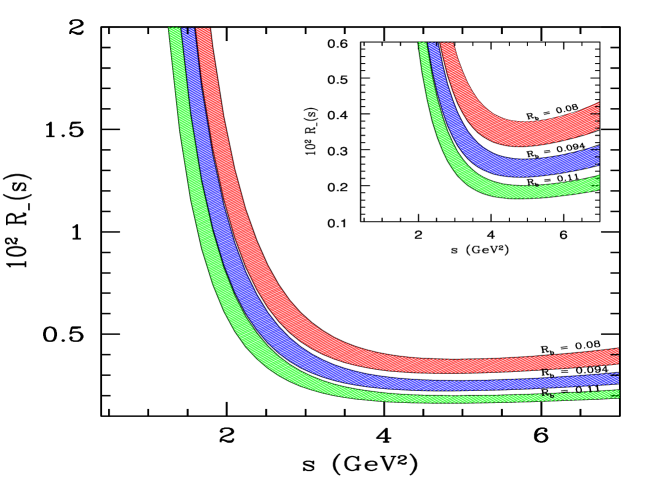
Figure 3.27: The Ratio $R_{-}(s)$ with three indicated values of the CKM ratio $R_{b}\equiv|V_{ub}|/|V_{tb}V_{ts}^{*}|$. The bands reflect the theoretical uncertainty from $\zeta_{SU(3)}=1.3\pm 0.06$ and $\xi^{(K^{*})}_{{\perp}}(0)=0.28\pm 0.04$ [28].

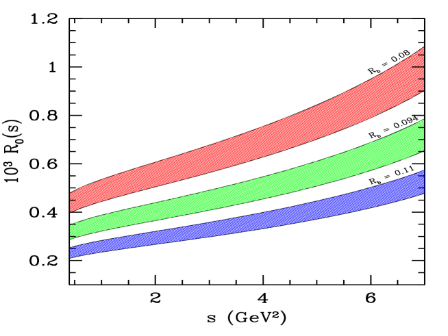
Figure 3.28: The Ratio $R_{0}(s)$ with three indicated values of the CKM ratio $R_{b}\equiv|V_{ub}|/|V_{tb}V_{ts}^{*}|$. The bands reflect the theoretical uncertainty from $\zeta_{SU(3)}=1.3\pm 0.06$ and $\xi^{(K^{*})}_{{\perp}}(0)=0.28\pm 0.04$ [28].

where the function ${\cal F}(s,m_{K^{*}},m_{\rho},...)$ denotes the kinematical contribution extracted from the ratio $|H_{i}^{(K^{*})}(s)|^{2}/|H_{i}^{(\rho)}(s)|^{2}$. Since the helicty amplitudes $H_{-}^{(K^{*})}(s)$ and $H_{-}^{(\rho)}(s)$ depend just on one universal form factor, respectively $\xi^{(K^{*})}_{\perp}$ and $\xi^{(\rho)}_{\perp}$, one can easily factorize apriori the ratio $R_{-}(s)$ as a kinematic contribution (expressed in ${\cal F}(s,m_{K^{*}},m_{\rho},...)$) and a dynamical contribution (encoded in the ratio of $\xi^{(K^{*})}_{\perp}/\xi^{(\rho)}_{\perp}$).

There is no doubt that in the SU(3) symmetry limit, the function $R_{-}(s)$ will be defined as a kinematical function and thus no uncertainty from the non-perturbative regime. Unhappily, the reality is far from being that, and one has to incorporate the SU(3)-breaking effects. Then the only source of uncertainty coming from the long distance contribution, will be translated in the ratio $\zeta_{SU(3)}=\xi^{(K^{*})}_{\perp}/\xi^{(\rho)}_{\perp}$, which turns out to be $\zeta_{SU(3)}=1.3\pm 0.06$, already defined in section 3.4.

On the other hand, the ratio $R_{0}(s)$ could bring a certain hint on the the structure of $R_{b}$. However its dependence on the form factors is more involved and cann’t be fudged away, as one can see:

$$R_{0}(s)\propto{1\over R_{b}^{2}}\,{|\xi^{(K^{*})}_{\perp}(s)\,\,{\cal F}_{1}^{(K^{*})}(s,m_{K^{*}},...)+\xi^{(K^{*})}_{||}(s)\,\,{\cal F}_{2}^{(K^{*})}(s,m_{K^{*}},...)|^{2}\over|\xi^{(\rho)}_{\perp}(s)\,\,{\cal F}_{1}^{(\rho)}(s,m_{\rho},...)+\xi^{(\rho)}_{||}(s)\,\,{\cal F}_{2}^{(\rho)}(s,m_{\rho},...)|^{2}},$$ (3.127)

where ${\cal F}_{1,2}^{(K^{*})}(s,m_{K^{*}},...)$ (${\cal F}_{1,2}^{(\rho)}(s,m_{K^{*}},...)$) are a certain dynamical function^≀ obtained from $|H_{0}^{K^{*}}(s)|^{2}$ ($|H_{0}^{\rho}(s)|^{2}$). Thus, we see that the ratio $R_{0}(s)$ is less attractive than the $R_{-}(s)$ ones for the extraction of the CKM ratio $R_{b}$, since its uncertainty is more poluated with the long distance contribution.

In Figs. (3.27) and (3.28) we plot $R_{-}(s)$ and $R_{0}(s)$ respectively, for three representative values of the CKM ratio $R_{b}=0.08$, $0.094$, and $0.11$. However, as we noticed earlier, the ratio $R_{-}(s)$ may be statistically limited due to the dominance of the decay $B\rightarrow\rho\ell\nu_{\ell}$ by the Helicity-$0$ component. For the LEET form factors used here, the compounded theoretical uncertainty is shown by the shaded regions. This figure suggests that high statistics experiments may be able to determine the CKM-ratio from measuring $R_{0}(s)$ at a competitive level compared to the other methods en vogue in experimental studies.

3.6 Summary and Outlook

In this Chapter we have investigated an $O(\alpha_{s})$-improved analysis of the various helicity components in the decays $B\rightarrow K^{*}\ell^{+}\ell^{-}$ and $B\rightarrow\rho\ell\nu_{\ell}$, carried out in the context of the Large-Energy-Effective-Theory. Using that and borrowing the corresponding form factors from QCD sum rule, we have investigated the corresponding distributions, decay rates and Forward-bckward asymmetry.

In the first part, we have concentrated mainly on the study of double and single angular distributions, and the FB asymmetry. Our findings can be summarized as follows [28]:

• We have calculated the helicity components implementing the $O(\alpha_{s})$ corrections and shown that the $+1$-helicity component is completely negligeable compared to the two other components, namely $H_{0}$ and $H_{-}$.

• The total dilepton invariant mass distribution ${d{\cal B}\over ds}$ is dominated by the partial single distribution ${d{\cal B}_{|H_{-}|^{2}}\over ds}$. The nex-to-leading order correction to the total dilepton invariant mass distribution is significant in the low dilepton mass region $(s\leq 2(\textrm{GeV}^{2}))$.

• We have shown that the $O(\alpha_{s})$ effects on the forward-backward asymmetry shifts the predicted location of its zero by $\sim 1~{}\textrm{GeV}^{2}$, confirming essentially the earlier work of Beneke, Feldmann and Seidel [25].

• We have carried out the $B\rightarrow K^{*}\ell^{+}\ell^{-}$ decay analysis in the so-called transversity basis. We have compared the LEET-based amplitudes in this basis with the data currently available on $B\rightarrow K^{*}J/\psi(\rightarrow\ell^{+}\ell^{-})$ and find that the short-distance based transversity amplitudes are very similar to their long-distance counterparts.

In the same spirit we have studied the $B\rightarrow\rho\ell\nu_{\ell}$ decay in the second part of this chapter, using the helicity analysis in the large energy effective theory . After presenting various double and single angular distributions, we summarize [28]:

• Considering the SU(3)-breaking effects, we have related the $B\rightarrow\rho\ell\nu_{\ell}$ LEET-form factors, namely $\xi^{(\rho)}_{\perp}(s)$ and $\xi^{(\rho)}_{||}(s)$, to the corresponding form factors in $B\rightarrow K^{*}\ell^{+}\ell^{-}$. Our numerical estimates on $\xi^{(\rho)}_{\perp}(s)$ and $\xi^{(\rho)}_{||}(s)$ are in agreement with the ones worked out for the full QCD form factors in the QCD sum-rule approach in [30].

• Implementing the $O(\alpha_{s})$ corrections to the $B\rightarrow\rho\ell\nu_{\ell}$ helicity components, we have shown that the $+1$-helicity component is completely negligeable compared to the two other components, namely $H_{0}$ and $H_{-}$.

• The total dilepton invariant mass distribution ${d{\cal B}\over ds}$ is dominated by the partial single distribution ${d{\cal B}_{|H_{0}|^{2}}\over ds}$. The nex-to-leading order correction to the total dilepton invariant mass distribution is completely negligeable.

Finally, combining the analysis of the decay modes $B\rightarrow K^{*}\ell^{+}\ell^{-}$ and $B\rightarrow\rho\ell\nu_{\ell}$, we have shown that the ratios of differential decay rates involving definite helicity states, $R_{-}(s)$ and $R_{0}(s)$, can be used for extracting the CKM matrix elements $|V_{ub}|/|V_{ts}|$ in a model-independent way.

Chapter 4 Exclusive $B\rightarrow\ K^{*}\ell^{+}\ell^{-}$ Decay in SUSY

This chapter is devoted to the semileptonic rare $B\rightarrow\ K^{*}\ell^{+}\ell^{-}$ decay, by contrasting its anticipated phenomenological profile in some variants of supersymmetric models. We discuss the constraints on the Wilson coefficients $C_{7}$, $C_{8}$, $C_{9}$ and $C_{10}$, that the current data on rare $B$ decays implies in the context of minimal flavour violating model and in more general scenarios admitting additional flavour changing mechanisms. As probes of new physics effects in $B\rightarrow\ K^{*}\ell^{+}\ell^{-}$, we propose to study the ratios $R_{0}(s)$ and $R_{-}(s)$ (introduced in the previous chapter) using some generic SUSY effects.

4.1 Introduction

Although the Standard Model (SM) of the elementary particle physics is successful in explaining almost all experimental results, it is possible that physics beyond the SM exists just above the presently available energy scale. Since new physics may affect various processes at low energy such as the flavor changing neutral current (FCNC) processes of $K$-mesons and $B$-mesons, new physics searches in these processes are as important as direct particle searches at collider experiments. A prime example is the $b\rightarrow s~{}\gamma$, process. Experimentally the current world average based on the improved measurements by the BABAR [11], CLEO [12], ALEPH [13] and BELLE [14] collaborations, ${\cal B}(B\rightarrow X_{s}\gamma)=(3.43^{+0.42}_{-0.37})\times 10^{-4}$. It is known that this process puts very strong constraints on various new physics beyond the SM, for example two Higgs doublet model and supersymmetric (SUSY) extension of the SM.

Along with the $b\rightarrow s~{}\gamma$ process, another important rare $b$ decay process is the $b\rightarrow s~{}\ell^{+}\ell^{-}$ decay. In particular, after the first measurements of the semileptonic rare $B$-decays reported in the inclusive $B\rightarrow X_{s}\ell^{+}\ell^{-}$ $(\ell^{\pm}=e^{\pm},\mu^{\pm})$ mode, with ${\cal B}(B\rightarrow X_{s}\ell^{+}\ell^{-})=(6.1\pm 1.4^{+1.3}_{-1.1})\times 10^{-6}$, by the BELLE collaboration [14] as well as the exclusive $B\rightarrow K^{*}\ell^{+}\ell^{-}$ $(\ell^{\pm}=e^{\pm},\mu^{\pm})$ one, typically ${\cal B}(B\rightarrow K^{*}\ell^{+}\ell^{-})=(1.68^{+0.68}_{-0.58}\pm 0.28)\times 10^{-6}$, by the BABAR collaboration [18].

With increased statistical power of experiments at the $B$-factories in the next several years, the decays discussed above and related rare $B$ decays will be measured very precisely. On the theoretical side, impressive progress in the theoretical precision has been achieved concerning the exclusive as well as the inclusive semileptonic (and radiative) rare $B$-decays, with the completion of NNLO (NLO) QCD calculations [?–?]. Although the theoretical uncertainties can be addressed only with a complete NLO, as $b\rightarrow s\gamma$ is calculated so far only in NLO , the SM value for the branching ratio is in agreement with the experimental measurement within the $1-2\sigma$ level.

Since the abovementioned FCNC rare $B$-processes are forbidden in the Born approximation any significant deviation from the SM would imply strongly the existence of new physics, such as Supersymmetry (SUSY). The reason is simply that, while in the SM the $b\rightarrow s$ transition are dominated by one loop contributions with the exchange of a virtual $W$ and the top quark, in SUSY [130, 131] several competing sources of FCNC are present. To begin with, in SUSY models the Higgs sector is richer than in the SM, since at least two Higgs doublets must be present. Consequently, there exists at least one physical charged scalar $H^{\pm}$ which can be exchanged in the one-loop contribution to $b\rightarrow s$, together with an up quark. The second obvious source of FCNC comes from the supersymmetrization of the W and the charged Higgs contributions, where the up quark is replaced by an up squark and $W$.

In this chapter we present a SUSY analysis of the semileptonic rare $B\rightarrow\ K^{*}\ell^{+}\ell^{-}$ decay, in the so-called minimal supersymmetric standard model (MSSM). After a brief review of the MSSM in section 4.2, we present in section 4.3 the allowed region of the SUSY parameter space. Section 4.4 shows the various supersymmetric contribution to the $b\rightarrow s~{}\ell^{+}\ell^{-}$ transition, while in section 4.5 we study the $B\rightarrow K^{*}\ell^{+}\ell^{-}$ decay in some specific SUSY-models, such as Minimal supergravity (mSUGRA) model, Minimal flavor violating supersymmetric model (MFV) and Extended Minimal flavor violating supersymmetric model (EMFV). As probes of new physics effects in $B\rightarrow\ K^{*}\ell^{+}\ell^{-}$, we propose in section 4.6 to study the ratios $R_{0}(s)$ and $R_{-}(s)$ (introduced and calculated in the SM in Chapter 3) in the generic mSUGRA model. Finally, we summarized our analysis in section 4.7.

4.2 The Minimal Supersymmetric Standard Model

The minimal supersymmetric standard model (MSSM) is the by far most widely studied potentially realistic SUSY model. It owes its popularity mostly to its simplicity, being essentially a straightforward supersymmetrization of the Standard Model (SM), where one introduces only those couplings and fields that are necessary for consistency [?–?].

The single-particle states of the MSSM fall naturally into irreducible representations of the corresponding algebra which are called supermultiplets. Each supermultiplet contains both fermion and boson states with the same electric charge, weak isospin, and color degrees of freedom, which are commonly known as superpartners of each other. All of the Standard Model fermions (the known quarks and leptons) are members of chiral supermultiplets. The names for the spin-0 partners of the quarks and leptons are constructed by prepending an “s”, which is short for scalar. It seems clear that the Higgs scalar boson must reside in a chiral supermultiplet, since it has spin 0. Actually, it turns out that one chiral supermultiplet is not enough. One way to see this is to note that if there were only one Higgs chiral supermultiplet, the electroweak gauge symmetry would suffer a triangle gauge anomaly, and would be inconsistent as a quantum theory.

The basic structure of the MSSM is well-known and has been thoroughly discussed in the literature [133, 134]. We therefore recall just those aspects of the theory which are pertinent to $b\rightarrow s~{}\ell^{+}\ell^{-}$ transitions. We first display nomenclature conventions for matter superfields and their left handed fermion and scalar components in Table 4.1, classified according to their transformation properties under the SM gauge group $SU(3)_{C}\times SU(2)_{L}\times U(1)_{Y}$.

Names		Fermions	Scalars
squarks, quarks	$Q_{i}=\pmatrix{U_{i}\cr D_{i}\cr}$	$q_{i}=\pmatrix{u_{i}\cr d_{i}\cr}$	$\tilde{q}_{i}=\pmatrix{\tilde{u}_{i}\cr\tilde{d}_{i}\cr}$
($\times 3$ families)	$U_{i}^{c}$	$u_{i}^{c}$	$\tilde{u}_{i}^{c}$
	$D_{i}^{c}$	$d_{i}^{c}$	$\tilde{d}_{i}^{c}$
sleptons, leptons	$L_{i}=\pmatrix{N_{i}\cr E_{i}\cr}$	$\ell_{i}=\pmatrix{\nu_{i}\cr e_{i}\cr}$	$\tilde{\ell}_{i}=\pmatrix{\tilde{\nu}_{i}\cr\tilde{e}_{i}\cr}$
($\times 3$ families)	$E_{i}^{c}$	$e_{i}^{c}$	$\tilde{e}_{i}^{c}$
Higgs, higgsinos	$H_{1}=\pmatrix{H^{0}_{1}\cr H^{-}_{1}\cr}$	$\tilde{h}_{1}=\pmatrix{\tilde{h}_{1}^{0}\cr\tilde{h}_{1}^{-}\cr}$	$h_{1}=\pmatrix{{h^{0}_{1}}^{*}\cr-h_{1}^{-}\cr}$
	$H_{2}=\pmatrix{H^{+}_{2}\cr H^{0}_{2}\cr}$	$\tilde{h}_{2}=\pmatrix{\tilde{h}_{2}^{+}\cr\tilde{h}_{2}^{0}\cr}$	$h_{2}=\pmatrix{h_{2}^{+}\cr h_{2}^{0}\cr}$

Table 4.1: Chiral supermultiplets in the Minimal Supersymmetric Standard Model.

The vector bosons of the SM clearly must reside in gauge supermultiplets. Their fermionic superpartners are generically referred to as gauginos. The $SU(3)_{C}$ color gauge interactions of QCD are mediated by the gluon, whose spin-1/2 color-octet supersymmetric partner is the gluino. As usual, a tilde is used to denote the supersymmetric partner of a SM state, so the symbols for the gluon and gluino are $g$ and $\tilde{g}$ respectively. The electroweak gauge symmetry $SU(2)_{L}\times U(1)_{Y}$ has associated with it spin-1 gauge bosons $W^{+},W^{0},W^{-}$ and $B^{0}$, with spin-1/2 superpartners $\tilde{W}^{+},\tilde{W}^{0},\tilde{W}^{-}$ and $\tilde{B}^{0}$, called winos and bino. After electroweak symmetry breaking, the $W^{0}$, $B^{0}$ gauge eigenstates mix to give mass eigenstates $Z^{0}$ and $\gamma$. The corresponding gaugino mixtures of $\tilde{W}^{0}$ and $\tilde{B}^{0}$ are called zino ($\tilde{Z}^{0}$) and photino ($\tilde{\gamma}$); if supersymmetry were unbroken, they would be mass eigenstates with masses $m_{Z}$ and 0. Table 4.2 summarizes the gauge supermultiplets of a minimal supersymmetric extension of the SM.

Names	Fermions	Vectors
gluino, gluon	$\tilde{g}$	$g$
winos, W bosons	$\tilde{W}^{\pm}\>\>\>\tilde{W}^{0}$	$W^{\pm}\>\>\>W^{0}$
bino, B boson	$\tilde{B}^{0}$	$B^{0}$

Table 4.2: Gauge supermultiplets in the Minimal Supersymmetric Standard Model.

After this brief introduction on the field content of the MSSM, we will review in what follows, the aspects of the theory relevant to the $b\rightarrow s~{}\ell^{+}\ell^{-}$ transitions considering only the case of unbroken R-parity. The superpotential which determines the supersymmetry preserving interactions among matter fields is:

$$W=\mu_{susy}~{}H_{1}H_{2}+Y^{\scriptscriptstyle U}_{ij}Q_{i}U^{c}_{j}H_{2}+Y^{\scriptscriptstyle D}_{ij}Q_{i}D^{c}_{j}H_{1}+Y^{\scriptscriptstyle E}_{ij}L_{i}E^{c}_{j}H_{1},$$ (4.1)

where $Q$, $U^{c}$, $D^{c}$, $L$ and $E^{c}$ are the superfields corresponding to the $SU(2)$ doublets and singlets for quarks and leptons, $H_{1}$ and $H_{2}$ are the two Higgs superfields, $Y^{f}$ are the Yukawa matrices and $\mu$ is the Higgs quadratic coupling. After vector superfield terms are included, the supersymmetric Lagrangian schematically appears in component form as [135]

$${\cal L}_{\rm SUSY} = -{1\over 4}{F_{\scriptscriptstyle G}^{\scriptscriptstyle A}}^{\mu\nu}{F_{\scriptscriptstyle G}^{\scriptscriptstyle A}}_{\mu\nu}+\overline{\lambda_{\scriptscriptstyle G}^{\scriptscriptstyle A}}iD\hskip-6.49994pt/\hskip 3.00003pt_{{\scriptscriptstyle A}{\scriptscriptstyle B}}\lambda_{\scriptscriptstyle G}^{\scriptscriptstyle B}+(D^{\mu}\phi)^{\dagger}(D_{\mu}\phi)+\overline{\psi}iD\hskip-6.49994pt/\hskip 3.00003pt\psi$$ (4.4)

$$-\left[\left({dW\over d\Phi_{i}}\right)^{*}\left({dW\over d\Phi_{i}}\right)+{\textstyle{1\over 2}}\left({\partial^{2}W\over\partial\Phi_{i}\partial\Phi_{j}}\psi_{i}^{\scriptscriptstyle T}C\psi_{j}+{\rm h.c.}\right)\right]_{\Phi\rightarrow\phi}$$

$$-\sqrt{2}g_{\scriptscriptstyle G}\left[\phi^{\dagger}T^{\scriptscriptstyle A}_{\scriptscriptstyle G}{\lambda^{\scriptscriptstyle A}_{\scriptscriptstyle G}}^{\scriptscriptstyle T}C\psi+{\rm h.c.}\right]-{\textstyle{1\over 2}}g^{2}_{\scriptscriptstyle G}(\phi^{\dagger}T^{\scriptscriptstyle A}_{\scriptscriptstyle G}\phi)(\phi^{\dagger}T^{\scriptscriptstyle A}_{\scriptscriptstyle G}\phi).$$

The index $G$ labels the color, weak isospin and hypercharge factors in the Standard Model gauge group, and indices $A$ and $B$ range over the nonabelian subgroups’ adjoint representations. All MSSM scalars are assembled into $\phi$, while matter fermions and gauginos are respectively contained within the four-component left handed $\psi$ and $\lambda$ fields.

Since supersymmetry is manifestly violated in the low energy world, the MSSM Lagrangian is supplemented with the soft supersymmetry breaking terms [135]

$${\cal L}_{\rm soft} = -{\textstyle{1\over 2}}\Bigl{[}m_{\tilde{g}}\tilde{g}^{a\,{\scriptscriptstyle T}}C\tilde{g}^{a}+m_{\tilde{{\scriptscriptstyle W}}}\tilde{W}^{i\,{\scriptscriptstyle T}}C\tilde{W}^{i}+m_{\tilde{{\scriptscriptstyle B}}}\tilde{B}^{\scriptscriptstyle T}C\tilde{B}+{\rm h.c.}\Bigr{]}-{\Delta}_{1}^{2}h_{1}^{\dagger}h_{1}-{\Delta}_{2}^{2}h_{2}^{\dagger}h_{2}$$ (4.7)

$$-\tilde{q}^{\dagger}_{i}(M^{2}_{\tilde{q}})_{ij}\tilde{q}_{j}-\tilde{u}^{c\,\dagger}_{i}(M^{2}_{\tilde{u}^{c}})_{ij}{\tilde{u}}^{c}_{j}-\tilde{d}^{c\,\dagger}_{i}(M^{2}_{\tilde{d}^{c}})_{ij}{\tilde{d}}^{c}_{j}-\tilde{\ell}^{\dagger}_{i}(M^{2}_{\tilde{\ell}})_{ij}\tilde{\ell}_{j}-\tilde{e}^{c\,\dagger}_{i}(M^{2}_{\tilde{e}^{c}})_{ij}{\tilde{e}}^{c}_{j}$$

$$+\Bigl{[}A^{\scriptscriptstyle U}_{ij}\tilde{q}_{i}\tilde{u}^{c}_{j}h_{2}+A^{\scriptscriptstyle D}_{ij}\tilde{q}_{i}\tilde{d}^{c}_{j}h_{1}+A^{\scriptscriptstyle E}_{ij}\tilde{\ell}_{i}\tilde{e}^{c}_{j}h_{1}+B\mu_{susy}h_{1}h_{2}+{\rm h.c.}\Bigr{]},$$

where $m_{\tilde{g}}$ ($m_{\tilde{{\scriptscriptstyle W}}}$ and $m_{\tilde{{\scriptscriptstyle B}}}$), ${\Delta}_{i}^{2}$ $(i=1,2)$ and $B\mu_{susy}$ are mass terms for gluino (wino and bino) and for the Higgs fields, respectively. The scalar mass terms $M^{2}_{\tilde{q}}$, $M^{2}_{\tilde{u}^{c}}$, $M^{2}_{\tilde{d}^{c}}$, $M^{2}_{\tilde{\ell}}$ and $M^{2}_{\tilde{e}^{c}}$ are in general hermitian $3\times 3$ matrices, while $A^{\scriptscriptstyle U}~{}h_{2}$, $A^{\scriptscriptstyle D}~{}h_{1}$ and $A^{\scriptscriptstyle E}~{}h_{1}$ are general $3\times 3$ matrices. Allowing all the parameters in (4.7) to be complex, we end up with 124 masses, phases and mixing angles as free parameters of the model.

Electroweak symmetry breaking induces mixing among MSSM fields. In the matter sector, primed mass eigenstates are related to unprimed gauge eigenstate counterparts as follows:

$$u^{\prime} = {\cal S}^{U_{L}}u+{\cal S}^{U_{R}}C{\overline{u^{c}}}^{\>{\scriptscriptstyle T}},~{}~{}~{}~{}~{}~{}~{}~{}~{}~{}~{}~{}~{}~{}~{}~{}~{}~{}~{}\tilde{u}^{\prime}={\cal T}^{U}\pmatrix{{\cal S}^{U_{L}}\>\tilde{u}\cr{\cal S}^{U_{R}}\>\tilde{u^{c}}^{*}\cr}$$

$$d^{\prime} = {\cal S}^{D_{L}}d-{\cal S}^{D_{R}}C{\overline{d^{c}}}^{\>{\scriptscriptstyle T}},~{}~{}~{}~{}~{}~{}~{}~{}~{}~{}~{}~{}~{}~{}~{}~{}~{}~{}~{}\tilde{d}^{\prime}={\cal T}^{D}\pmatrix{{\cal S}^{D_{L}}\>\tilde{d}\cr-{\cal S}^{D_{R}}\>\tilde{d^{c}}^{*}\cr}$$

$$\nu^{\prime} = {\cal S}^{N_{L}}\nu,~{}~{}~{}~{}~{}~{}~{}~{}~{}~{}~{}~{}~{}~{}~{}~{}~{}~{}~{}~{}~{}~{}~{}~{}~{}~{}~{}~{}~{}~{}~{}~{}~{}~{}~{}~{}~{}~{}~{}~{}\tilde{\nu}^{\prime}={\cal T}^{N}{\cal S}^{E_{L}}\tilde{\nu}$$

$$e^{\prime} = {\cal S}^{E_{L}}e-{\cal S}^{E_{R}}C{\overline{e^{c}}}^{\>{\scriptscriptstyle T}},~{}~{}~{}~{}~{}~{}~{}~{}~{}~{}~{}~{}~{}~{}~{}~{}~{}~{}~{}\tilde{e}^{\prime}={\cal T}^{E}\pmatrix{{\cal S}^{E_{L}}\>\tilde{e}\cr-{\cal S}^{E_{R}}\>\tilde{e^{c}}^{*}\cr}.$$ (4.8)

The unitary ${\cal S}$ and ${\cal T}$ transformations rotate fermion and sfermion mass matrices into real and diagonal forms. The $3\times 3$ quark and lepton mass matrices are simply related to the Yukawa couplings in the superpotential:

$$M_{U} = {v\sin\beta\over\sqrt{2}}{\cal S}^{U_{R}}{Y^{U}}^{\scriptscriptstyle T}{{\cal S}^{U_{L}}}^{\dagger}$$

$$M_{D} = {v\cos\beta\over\sqrt{2}}{\cal S}^{D_{R}}{Y^{D}}^{\scriptscriptstyle T}{{\cal S}^{D_{L}}}^{\dagger}$$

$$M_{E} = {v\cos\beta\over\sqrt{2}}{\cal S}^{E_{R}}{Y^{E}}^{\scriptscriptstyle T}{{\cal S}^{E_{L}}}^{\dagger},$$ (4.9)

where $v_{1}=v\cos\beta$ and $v_{2}=v\sin\beta$ are the expectation values of the two Higgs doublets and ${\cal S}^{f}~{}\big{(}f=U_{R},U_{L},D_{R},D_{L},E_{R},E_{L}\big{)}$. The $6\times 6$ squared mass matrices for the squarks (we do not present the lepton ones since they are not relevant for the forthcoming analysis of SUSY contributions) read:

$$M^{2}_{\tilde{u}} = {\cal T}^{U}\left(\begin{array}[]{cc}{\cal S}^{U_{L}}M^{2}_{\tilde{q}}{{\cal S}^{U_{L}}}^{\dagger}+M_{U}^{2}+\ldots&\mu_{susy}M_{U}\cot\beta-\displaystyle{v\sin\beta\over\sqrt{2}}{\cal S}^{U_{L}}{A^{U}}^{*}{{\cal S}^{U_{R}}}^{\dagger}\\ \mu_{susy}^{*}M_{U}\cot\beta-\displaystyle{v\sin\beta\over\sqrt{2}}{\cal S}^{U_{R}}{A^{U}}^{\scriptscriptstyle T}{{\cal S}^{U_{L}}}^{\dagger}&{\cal S}^{U_{R}}{M^{2}_{\tilde{u}^{c}}}^{\scriptscriptstyle T}{{\cal S}^{U_{R}}}^{\dagger}+M_{U}^{2}+\ldots\end{array}\right){{\cal T}^{U}}^{\dagger}$$ (4.12)

$$M_{\tilde{d}}^{2} = {\cal T}^{D}\left(\begin{array}[]{cc}{\cal S}^{D_{L}}\,M_{\tilde{q}}^{2}\,{{\cal S}^{D_{L}}}^{\dagger}+M_{D}^{2}+\ldots&\mu_{susy}M_{D}\tan\beta-\displaystyle{v\cos\beta\over\sqrt{2}}{\cal S}^{D_{L}}\,{A^{D}}^{*}\,{{\cal S}^{D_{R}}}^{\dagger}\\ \mu^{*}_{susy}M_{D}\tan\beta-\displaystyle{v\cos\beta\over\sqrt{2}}{\cal S}^{D_{R}}\,A^{D^{T}}\,{{\cal S}^{D_{L}}}^{\dagger}&{\cal S}^{D_{R}}\,{M^{2}_{\tilde{d}^{c}}}^{\scriptscriptstyle T}\,{{\cal S}^{D_{R}}}^{\dagger}+M_{D}^{2}+\ldots\end{array}\right){{\cal T}^{D{\dagger}}},$$ (4.15)

where $M^{2}_{\tilde{u}}$ and $M_{\tilde{d}}^{2}$ are the diagonal mass matrices of the up and down squarks and the dots stand for terms proportional to $m^{2}_{Z}$. Moreover, $M^{2}_{\tilde{u}}$ and $M_{\tilde{d}}^{2}$ are matrices in the basis in which the squark fields undergo the same rotations as the quark ones. This means that we diagonalize the matrices $M_{U}$ and $M_{D}$ applying rigid rotations to the quark superfields and that there is not any flavour change in vertices with both quark and squarks. In the literature this basis is usually referred as the SuperCKM (SCKM) one.

Mixing also takes place in the gaugino and Higgs sectors. The physical Dirac chargino and Majorana neutralino eigenstates are respectively linear combinations of left handed Winos, Binos and Higgsinos. Thus in the weak eigenstates basis, the chargino and neutalino mass matrices are given respectively, by

$$M_{\tilde{\chi}^{\pm}} ={\cal U}^{*}\left(\begin{array}[]{cc}m_{\tilde{{\scriptscriptstyle W}}}&\sqrt{2}m_{W}\sin\beta\\ \sqrt{2}m_{W}\cos\beta&-\mu_{susy}\end{array}\right){\cal V}^{\dagger},$$ (4.19)

and

$$M_{\tilde{\chi}^{0}} ={\cal N}^{*}\pmatrix{m_{\tilde{{\scriptscriptstyle B}}}&0&-m_{Z}\sin\theta\cos\beta&m_{Z}\sin\theta\sin\beta\cr 0&m_{\tilde{{\scriptscriptstyle W}}}&m_{Z}\cos\theta\cos\beta&-m_{Z}\cos\theta\sin\beta\cr-m_{Z}\sin\theta\cos\beta&m_{Z}\cos\theta\cos\beta&0&\mu_{susy}\cr m_{Z}\sin\theta\sin\beta&-m_{Z}\cos\theta\sin\beta&\mu_{susy}&0\cr}{\cal N}^{\dagger},$$

where, the unitary transformations ${\cal U}$, ${\cal V}$ and ${\cal N}$ are unitary matrices, which diagonalize these fields mass matrices.

After the gauge eigenstate fields in the supersymmetric Lagrangian 4.4 are rewritten in terms of their mass eigenstate counterparts, it is straightforward to work out the interactions of gluinos, charginos and neutralinos with quarks and squarks. We list below the resulting terms which participate at one-loop order in $d_{i}\rightarrow d_{j}\ell^{+}\ell^{-}$ decay:

$${\cal L}_{\tilde{g},\tilde{\chi}} = -\sqrt{2}g_{3}\sum_{a=1}^{8}\overline{\tilde{g}^{a}_{\scriptscriptstyle M}}\tilde{d}^{\dagger}({\cal T}^{D_{L}}L-{\cal T}^{D_{R}}R)T^{a}d$$ (4.22)

$$+\sum_{{\scriptscriptstyle I}=1}^{2}\overline{\tilde{\chi}}^{\,-}_{\scriptscriptstyle I}\tilde{u}^{\dagger}({\cal X}_{\scriptscriptstyle I}^{U_{L}}L+{\cal X}_{\scriptscriptstyle I}^{U_{R}}R)d+\sum_{{\scriptscriptstyle I}=1}^{4}(\overline{\tilde{\chi}}^{0}_{\scriptscriptstyle M})_{\scriptscriptstyle I}\tilde{d}^{\dagger}({\cal Z}_{\scriptscriptstyle I}^{D_{L}}L+{\cal Z}_{\scriptscriptstyle I}^{D_{R}}R)d+{\rm h.c.},$$

where

$${\cal X}_{\scriptscriptstyle I}^{U_{L}} = g_{2}\Bigl{(}-{\cal V}^{*}_{{\scriptscriptstyle I}1}{\cal T}^{U_{L}}+{\cal V}^{*}_{{\scriptscriptstyle I}2}{\cal T}^{U_{R}}{M_{\scriptscriptstyle U}\over\sqrt{2}m_{W}\sin\beta}\Bigr{)}V_{\mathrm{C}KM},$$

$${\cal X}_{\scriptscriptstyle I}^{U_{R}} = g_{2}\Bigl{(}{\cal U}_{{\scriptscriptstyle I}2}{\cal T}^{U_{L}}V_{\mathrm{C}KM}{M_{\scriptscriptstyle D}\over\sqrt{2}m_{W}\cos\beta}\Bigr{)},$$

$${\cal Z}_{\scriptscriptstyle I}^{D_{L}} = -{g_{2}\over\sqrt{2}}\Bigl{[}(-{\cal N}^{*}_{{\scriptscriptstyle I}2}+{1\over 3}\tan\theta{\cal N}^{*}_{{\scriptscriptstyle I}1}){\cal T}^{D_{L}}+{\cal N}^{*}_{{\scriptscriptstyle I}3}{\cal T}^{D_{R}}{M_{\scriptscriptstyle D}\over m_{W}\cos\beta}\Bigr{]},$$

$${\cal Z}_{\scriptscriptstyle I}^{D_{R}} = -{g_{2}\over\sqrt{2}}\Bigl{(}{2\over 3}\tan\theta{\cal N}_{{\scriptscriptstyle I}1}{\cal T}^{D_{R}}+{\cal N}_{{\scriptscriptstyle I}3}{\cal T}^{D_{L}}{M_{\scriptscriptstyle D}\over m_{W}\cos\beta}\Bigr{)}.$$ (4.23)

We see clearly that the flavor mixing enters into these interactions through the Kobayashi-Maskawa matrix $V_{\tiny{CKM}}={\cal S}^{U_{L}}{{\cal S}^{D_{L}}}^{\dagger}$ and the $6\times 3$ block components of ${\cal T}^{\scriptscriptstyle U}$ and ${\cal T}^{\scriptscriptstyle D}$:

$${\mathcal{T}}^{{\scriptscriptstyle U}(D)}_{6\times 6}=\Big{(}{\cal T}^{{U_{L}}({D_{L}})}_{6\times 3},{\cal T}^{{U_{R}}({D_{R}})}_{6\times 3}\Big{)}.$$ (4.24)

The Feynman rules for all these interactions may be found in the literature [133, 136]. Having set up the basic MSSM framework, we are now ready to explore its large parameter space. We take up this topic in the following section.

4.3 MSSM parameter space

Before predictions can be derived from the Minimal Supersymmetric Standard Model, explicit values for the parameters in the superpotential (4.1) and soft supersymmetry breaking Lagrangian (4.7) must be specified.

In order to determine the allowed region of the SUSY parameter space, we require the following phenomenological constraints[36]

1. $b\rightarrow s\gamma$ constraint from BABAR [11], CLEO [12], ALEPH [13] and BELLE [14] collaborations, i.e., $3.06\times 10^{-4}<{\cal B}(B\rightarrow X_{s}\gamma)<3.85\times 10^{-4}$.

2. From the recent experiment at LEP 2[36], we impose that all the charged SUSY particles are heavier than 70 GeV

3. The neutarlino ${\tilde{\chi}}_{1}^{0}$ mass is larger than 32 GeV.

4. All sneutrino masses are larger than 43 GeV [36].

5. The gluino and squark mass bounds from Fermilab Tevatron experiments [137]. The precise bounds on the gluino mass and the averaged squark mass except for the top squark is restricted to be larger than about 180 GeV.

6. The stop ${\tilde{t}}_{1}$ mass is larger than 87 GeV.

Having these phenomenological constraints at hand, let’s explore the SUSY contributions to the $b\rightarrow s\ell^{+}\ell^{-}$ transition.

4.4 Supersymmetric contribution to $b\rightarrow s~{}\ell^{+}\ell^{-}$

The Major theoretical breakthrough in the analysis of the FCNC tests in SUSY models came in 1983 when Duncan [139] and, independentely, Donoghue, Nilles and Wyler [140] noticed that FC transitions could occur at the $\tilde{g}-\tilde{q}-q$ vertices. The replacement of the weak coupling of the W with the strong coupling of the gluino, and the presence of approximately the same CKM mixing angles, raised the hope of possible SUSY enhancements of FCNC processes through one-loop gluino exchanges. Indeed, in the general context of MSSMs, it was found that these gluino mediated FCNC contributions could play a relevant role in CP violation of the K-system [141] and, more recently, in the radiative $b\rightarrow s\gamma$ [142] and $b\rightarrow sg$ [143] decays.

Within the MSSM, the $b\rightarrow s~{}\ell^{+}\ell^{-}$ transition is governed by five possible classes of contributions. They correspond to four classes of one loop SUSY diagrams that produce $b\rightarrow s~{}\ell^{+}\ell^{-}$ transition, in additions to W-exchange. We will classify them according to the particles running in the loop:

1. $W^{-}$ and up quarks (SM),

2. $H^{-}$ and up quarks,

3. $\tilde{\chi}^{-}$ and up squarks,

4. $\tilde{g}$ and down squarks,

5. $\tilde{\chi}^{0}$ and down squarks.

We list below the $W$-scale matching contributions to the Wilson coefficients $C_{7}$, $C_{9}$ and $C_{10}$ which arise from one-loop MSSM diagrams, presented in Fig. (4.1) and (4.2). The total contribution to $C_{i}$ $(i=7,9,10)$ and the normalized ratio can thus be written respectively as

$$C_{i}^{tot}(m_{W}) = C_{i}^{SM}(m_{W})+C_{i}^{NP}(m_{W}),$$ (4.25)

and

$$R_{i}={C_{i}^{tot}(m_{W})\over C_{i}^{SM}(m_{W})}.$$ (4.26)

We start with the $W$-scale matching contributions to the coefficient $C_{7}$ of the magnetic moment operator in the $\Delta B=1$ effective Hamiltonian which arise from one-loop MSSM diagrams, presented in Fig. (4.1) (only the $\gamma$-penguin diagrams). Thus its total contribution reads as

$$C_{7}^{tot}(m_{W}) = C_{7}^{SM}(m_{W})+C_{7}^{NP}(m_{W}),$$ (4.27)

where $C_{7}^{NP}(m_{W})$ represent the new physics contribution at the scale $m_{W}$ to the $C_{7}$, defined as:

$$C_{7}^{NP}(m_{W})=\delta C_{7}^{h_{\pm}}(m_{W})+\delta C_{7}^{\tilde{\chi}^{\pm}}(m_{W})+\delta C_{7}^{\tilde{\chi}^{0}}(m_{W})+\delta C_{7}^{\tilde{g}}(m_{W}).$$ (4.28)

The explicit expressions for the various terms are [135]:

• Standard Model graphs:

  $$C_{7}^{SM}={x_{t}\over 4}f_{1}(x_{t})$$ (4.29)

• Graphs with charged Higgs loops:

  $$\delta C_{7}^{h_{\pm}} ={1\over 6}\left\{{\textstyle{1\over 2}}{m_{t}^{2}\over m^{2}_{h^{\pm}}}\cot^{2}\beta\,f_{1}\bigl{(}{m_{t}^{2}\over m^{2}_{h^{\pm}}}\bigr{)}+f_{2}\bigl{(}{m_{t}^{2}\over m^{2}_{h^{\pm}}}\bigr{)}\right\}$$ (4.30)

• Graphs with chargino loops:

  $$\delta C_{7}^{\tilde{\chi}^{\pm}} = {1\over 3g_{2}^{2}V^{*}_{ts}V_{tb}}\sum_{{\scriptscriptstyle A}=1}^{6}\sum_{{\scriptscriptstyle I}=1}^{2}{m_{W}^{2}\over m_{\tilde{\chi}^{\pm}_{\scriptscriptstyle I}}^{2}}$$

  $$\qquad\times\Bigl{\{}-{\textstyle{1\over 2}}({\cal X}_{\scriptscriptstyle I}^{U_{L}})^{\dagger}_{\scriptscriptstyle 2A}({\cal X}_{\scriptscriptstyle I}^{U_{L}})_{\scriptscriptstyle A3}f_{1}\Bigl{(}{m_{\tilde{u}_{A}}^{2}\over m_{\tilde{\chi}^{\pm}_{\scriptscriptstyle I}}^{2}}\Bigr{)}+({\cal X}_{\scriptscriptstyle I}^{U_{L}})^{\dagger}_{\scriptscriptstyle 2A}({\cal X}_{\scriptscriptstyle I}^{U_{R}})_{\scriptscriptstyle A3}{m_{\tilde{\chi}^{\pm}_{\scriptscriptstyle I}}\over m_{b}}f_{2}\Bigl{(}{m_{\tilde{u}_{A}}^{2}\over m_{\tilde{\chi}^{\pm}_{\scriptscriptstyle I}}^{2}}\Bigr{)}\Bigr{\}}$$

• Graphs with neutralino loops:

  $$\delta C_{7}^{\tilde{\chi}^{0}} = -{1\over 3g_{2}^{2}V^{*}_{ts}V_{tb}}\sum_{{\scriptscriptstyle A}=1}^{6}\sum_{{\scriptscriptstyle I}=1}^{4}{m_{W}^{2}\over m_{\tilde{\chi}^{0}_{\scriptscriptstyle I}}^{2}}$$

  $$\qquad\times\Bigl{\{}{\textstyle{1\over 2}}({\cal Z}_{\scriptscriptstyle I}^{D_{L}})^{\dagger}_{\scriptscriptstyle 2A}({\cal Z}_{\scriptscriptstyle I}^{D_{L}})_{\scriptscriptstyle A3}f_{3}\Bigl{(}{m_{\tilde{d}_{A}}^{2}\over m_{\tilde{\chi}^{0}_{\scriptscriptstyle I}}^{2}}\Bigr{)}+({\cal Z}_{\scriptscriptstyle I}^{D_{L}})^{\dagger}_{\scriptscriptstyle 2A}({\cal Z}_{\scriptscriptstyle I}^{D_{R}})_{\scriptscriptstyle A3}{m_{\tilde{\chi}^{0}_{\scriptscriptstyle I}}\over m_{b}}f_{4}\Bigl{(}{m_{\tilde{d}_{A}}^{2}\over m_{\tilde{\chi}^{0}_{\scriptscriptstyle I}}^{2}}\Bigr{)}\Bigr{\}}$$

• Graphs with gluino loops:

  $$\delta C_{7}^{\tilde{g}} = {4g_{3}^{2}\over 9g_{2}^{2}V^{*}_{ts}V_{tb}}\sum_{{\scriptscriptstyle A}=1}^{6}{m_{W}^{2}\over m_{\tilde{g}}^{2}}$$

  $$\qquad\times\Bigl{\{}-({\cal T}^{D_{L}})^{\dagger}_{\scriptscriptstyle 2A}({\cal T}^{D_{L}})_{\scriptscriptstyle A3}f_{3}\Bigl{(}{m_{\tilde{d}_{A}}^{2}\over m_{\tilde{g}}^{2}}\Bigr{)}+2({\cal T}^{D_{L}})^{\dagger}_{\scriptscriptstyle 2A}({\cal T}^{D_{R}})_{\scriptscriptstyle A3}{m_{\tilde{g}}\over m_{b}}f_{4}\Bigl{(}{m_{\tilde{d}_{A}}^{2}\over m_{\tilde{g}}^{2}}\Bigr{)}\Bigr{\}}$$

The one-loop integral functions which enter into these matching conditions are given in Appendix C. Concerning the SUSY contributions to the chromo-magnetic coefficient $C_{8}$, it has the same structure as the $C_{7}$ ones, with different colour factors and loop-functions.

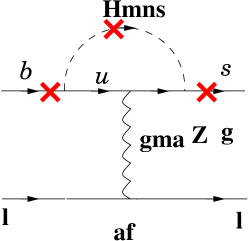
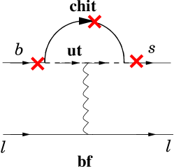
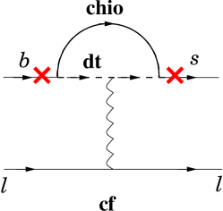
Figure 4.1: SUSY-Penguin diagrams relevant to the semileptonic $b\rightarrow s~{}\ell^{+}\ell^{-}$ transition in the MSSM. The cross denotes a possibility to attach the photon or the $Z$-boson.

Figure 4.2: SUSY-Box diagrams relevant to the semileptonic $b\rightarrow s~{}\ell^{+}\ell^{-}$ transition in the MSSM. The bubble in figure $(d)$ reflect the Majorana nature of the neutralinos.

The $W$-scale matching contributions to the semileptonic coefficients , namely $C_{9}^{eff}$ and $C_{10}$, which arise from one-loop MSSM diagrams, presented in Figs. (4.1) and (4.2), and can be written respectively as

$$C_{9,10}^{tot}(m_{W})=C_{9,10}^{SM}(m_{W})+C_{9,10}^{NP}(m_{W}),$$ (4.34)

where the SUSY contributuions to the semileptonic coefficients, are defined as:

$$C_{9}^{NP}(m_{W}) = \delta C_{9}^{(Z,\gamma)-peng,(H,\tilde{\chi},\tilde{\chi}^{0},\tilde{g})}+\delta C_{9}^{{}^{\prime}(Z,\gamma)-peng,(H,\tilde{\chi},\tilde{\chi}^{0},\tilde{g})}+\delta C_{9}^{(\tilde{\chi},\tilde{\chi}^{0})-box}+\delta C_{9}^{{}^{\prime}(\tilde{\chi},\tilde{\chi}^{0})-box},$$

$$C_{10}^{NP}(M_{W}) = C_{10}^{(Z,\gamma)-peng,(H,\tilde{\chi},\tilde{\chi}^{0},\tilde{g})}+\delta C_{10}^{(\tilde{\chi},\tilde{\chi}^{0})-box}.$$ (4.35)

The various terms are given as follow [135]:

• Z-penguin graphs with charged Higgs loops:

  $$\delta C_{9,10}^{Z-peng,H} = \mp{1\over 8~{}\sin^{2}\theta_{W}}\cot^{2}\beta\,x_{t}f_{5}\bigl{(}{m_{t}^{2}\over m^{2}_{h^{\pm}}}\bigr{)}$$

  $$\delta C_{9}^{{}^{\prime}Z-peng,H} = {1\over 2}\cot^{2}\beta\,x_{t}f_{5}\bigl{(}{m_{t}^{2}\over m^{2}_{h^{\pm}}}\bigr{)}$$ (4.36)

• $\gamma$-penguin graphs with charged Higgs loops:

  $$\delta C_{9,10}^{\gamma-peng,H} = 0$$

  $$\delta C_{9}^{{}^{\prime}\gamma-peng,H} = {1\over 18}\cot^{2}\beta\,f_{6}\bigl{(}{m_{t}^{2}\over m^{2}_{h^{\pm}}}\bigr{)}$$ (4.37)

• Z-penguin graphs with chargino loops:

  $$\delta C_{9,10}^{Z-peng,\tilde{\chi}}=\pm{1\over 2g_{2}^{2}~{}\sin^{2}\theta_{W}V^{*}_{ts}V_{tb}}\sum_{{\scriptscriptstyle A},{\scriptscriptstyle B}=1}^{6}\sum_{{\scriptscriptstyle I},{\scriptscriptstyle J}=1}^{2}({\cal X}_{\scriptscriptstyle I}^{U_{L}})^{\dagger}_{\scriptscriptstyle 2A}({\cal X}_{\scriptscriptstyle J}^{U_{L}})_{\scriptscriptstyle Bi}$$

  $$\qquad\times\Bigl{\{}c_{2}(m_{\tilde{\chi}^{\pm}_{\scriptscriptstyle I}}^{2},m_{\tilde{u}_{A}}^{2},m_{\tilde{u}_{B}}^{2})({\cal T}^{U_{L}}{{\cal T}^{U_{L}}}^{\dagger})_{{\scriptscriptstyle A}{\scriptscriptstyle B}}\,\delta_{{\scriptscriptstyle I}{\scriptscriptstyle J}}-c_{2}(m_{\tilde{u}_{A}}^{2},m_{\tilde{\chi}^{\pm}_{\scriptscriptstyle I}}^{2},m_{\tilde{\chi}^{\pm}_{\scriptscriptstyle J}}^{2})~{}\delta_{{\scriptscriptstyle A}{\scriptscriptstyle B}}~{}{\cal V}^{*}_{{\scriptscriptstyle I}1}~{}{\cal V}_{{\scriptscriptstyle J}1}$$

  $$\qquad+{\textstyle{1\over 2}}~{}m_{\tilde{\chi}^{\pm}_{\scriptscriptstyle I}}~{}m_{\tilde{\chi}^{\pm}_{\scriptscriptstyle J}}~{}c_{0}(m_{\tilde{u}_{A}}^{2},m_{\tilde{\chi}^{\pm}_{\scriptscriptstyle I}}^{2},m_{\tilde{\chi}^{\pm}_{\scriptscriptstyle J}}^{2})~{}\delta_{{\scriptscriptstyle A}{\scriptscriptstyle B}}~{}{\cal U}_{{\scriptscriptstyle I}1}~{}{\cal U}^{*}_{{\scriptscriptstyle J}1}\Bigr{\}}$$

  $$\delta C_{9}^{{}^{\prime}Z-peng,\tilde{\chi}}=-{2\over g_{2}^{2}V^{*}_{ts}V_{tb}}\sum_{{\scriptscriptstyle A},{\scriptscriptstyle B}=1}^{6}\sum_{{\scriptscriptstyle I},{\scriptscriptstyle J}=1}^{2}({\cal X}_{\scriptscriptstyle I}^{U_{L}})^{\dagger}_{\scriptscriptstyle 2A}({\cal X}_{\scriptscriptstyle J}^{U_{L}})_{\scriptscriptstyle Bi}$$

  $$\qquad\times\Bigl{\{}c_{2}(m_{\tilde{\chi}^{\pm}_{\scriptscriptstyle I}}^{2},m_{\tilde{u}_{A}}^{2},m_{\tilde{u}_{B}}^{2})~{}({\cal T}^{U_{L}}{{\cal T}^{U_{L}}}^{\dagger})_{{\scriptscriptstyle A}{\scriptscriptstyle B}}\,\delta_{{\scriptscriptstyle I}{\scriptscriptstyle J}}-c_{2}(m_{\tilde{u}_{A}}^{2},m_{\tilde{\chi}^{\pm}_{\scriptscriptstyle I}}^{2},m_{\tilde{\chi}^{\pm}_{\scriptscriptstyle J}}^{2})~{}\delta_{{\scriptscriptstyle A}{\scriptscriptstyle B}}~{}{\cal V}^{*}_{{\scriptscriptstyle I}1}~{}{\cal V}_{{\scriptscriptstyle J}1}$$

  $$\qquad+{\textstyle{1\over 2}}~{}m_{\tilde{\chi}^{\pm}_{\scriptscriptstyle I}}~{}m_{\tilde{\chi}^{\pm}_{\scriptscriptstyle J}}~{}c_{0}(m_{\tilde{u}_{A}}^{2},m_{\tilde{\chi}^{\pm}_{\scriptscriptstyle I}}^{2},m_{\tilde{\chi}^{\pm}_{\scriptscriptstyle J}}^{2})~{}\delta_{{\scriptscriptstyle A}{\scriptscriptstyle B}}~{}{\cal U}_{{\scriptscriptstyle I}1}~{}{\cal U}^{*}_{{\scriptscriptstyle J}1}\Bigr{\}}$$ (4.38)

• $\gamma$-penguin graphs with chargino loops:

  $$\delta C_{9,10}^{\gamma-peng,\tilde{\chi}} = 0$$

  $$\delta C_{9}^{{}^{\prime}\gamma-peng,\tilde{\chi}} = -{1\over 4g_{2}^{2}V^{*}_{ts}V_{tb}}\sum_{{\scriptscriptstyle A}=1}^{6}\sum_{{\scriptscriptstyle I}=1}^{2}{m_{W}^{2}\over m_{\tilde{u}_{A}}^{2}}({\cal X}_{\scriptscriptstyle I}^{U_{L}})^{\dagger}_{\scriptscriptstyle 2A}({\cal X}_{\scriptscriptstyle I}^{U_{L}})_{\scriptscriptstyle Ai}f_{7}\bigl{(}{m_{\tilde{\chi}^{\pm}_{\scriptscriptstyle I}}^{2}\over m_{\tilde{u}_{A}}^{2}}\bigr{)}$$ (4.39)

• Z-penguin graphs with neutralino loops:

  $$\delta C_{9,10}^{Z-peng,\tilde{\chi}^{0}}=\pm{1\over 2g_{2}^{2}~{}\sin^{2}\theta_{W}V^{*}_{ts}V_{tb}}\sum_{{\scriptscriptstyle A},{\scriptscriptstyle B}=1}^{6}\sum_{{\scriptscriptstyle I},{\scriptscriptstyle J}=1}^{4}({\cal Z}_{\scriptscriptstyle I}^{D_{L}})^{\dagger}_{\scriptscriptstyle 2A}({\cal Z}_{\scriptscriptstyle J}^{D_{L}})_{\scriptscriptstyle Bi}$$

  $$\quad\times\Bigl{\{}c_{2}(m_{\tilde{\chi}^{0}_{\scriptscriptstyle I}}^{2},m_{\tilde{d}_{A}}^{2},m_{\tilde{d}_{B}}^{2})({\cal T}^{D_{R}}{{\cal T}^{D_{R}}}^{\dagger})_{{\scriptscriptstyle A}{\scriptscriptstyle B}}\,\delta_{{\scriptscriptstyle I}{\scriptscriptstyle J}}-c_{2}(m_{\tilde{d}_{A}}^{2},m_{\tilde{\chi}^{0}_{\scriptscriptstyle I}}^{2},m_{\tilde{\chi}^{0}_{\scriptscriptstyle J}}^{2})~{}\delta_{{\scriptscriptstyle A}{\scriptscriptstyle B}}~{}({\cal N}^{*}_{{\scriptscriptstyle I}3}{\cal N}_{{\scriptscriptstyle J}3}-{\cal N}^{*}_{{\scriptscriptstyle I}4}{\cal N}_{{\scriptscriptstyle J}4})$$

  $$\quad-{\textstyle{1\over 2}}~{}m_{\tilde{\chi}^{0}_{\scriptscriptstyle I}}~{}m_{\tilde{\chi}^{0}_{\scriptscriptstyle J}}~{}c_{0}(m_{\tilde{d}_{A}}^{2},m_{\tilde{\chi}^{0}_{\scriptscriptstyle I}}^{2},m_{\tilde{\chi}^{0}_{\scriptscriptstyle J}}^{2})~{}\delta_{{\scriptscriptstyle A}{\scriptscriptstyle B}}~{}({\cal N}_{{\scriptscriptstyle I}3}{\cal N}^{*}_{{\scriptscriptstyle J}3}-{\cal N}_{{\scriptscriptstyle I}4}{\cal N}^{*}_{{\scriptscriptstyle J}4})\Bigl{\}}$$

  $$\delta C_{9}^{{}^{\prime}Z-peng,\tilde{\chi}^{0}}=-{2\over g_{2}^{2}V^{*}_{ts}V_{tb}}\sum_{{\scriptscriptstyle A},{\scriptscriptstyle B}=1}^{6}\sum_{{\scriptscriptstyle I},{\scriptscriptstyle J}=1}^{4}({\cal Z}_{\scriptscriptstyle I}^{D_{L}})^{\dagger}_{\scriptscriptstyle 2A}({\cal Z}_{\scriptscriptstyle J}^{D_{L}})_{\scriptscriptstyle Bi}$$

  $$\quad\times\Bigl{\{}c_{2}(m_{\tilde{\chi}^{0}_{\scriptscriptstyle I}}^{2},m_{\tilde{d}_{A}}^{2},m_{\tilde{d}_{B}}^{2})({\cal T}^{D_{R}}{{\cal T}^{D_{R}}}^{\dagger})_{{\scriptscriptstyle A}{\scriptscriptstyle B}}\,\delta_{{\scriptscriptstyle I}{\scriptscriptstyle J}}-c_{2}(m_{\tilde{d}_{A}}^{2},m_{\tilde{\chi}^{0}_{\scriptscriptstyle I}}^{2},m_{\tilde{\chi}^{0}_{\scriptscriptstyle J}}^{2})~{}\delta_{{\scriptscriptstyle A}{\scriptscriptstyle B}}~{}({\cal N}^{*}_{{\scriptscriptstyle I}3}{\cal N}_{{\scriptscriptstyle J}3}-{\cal N}^{*}_{{\scriptscriptstyle I}4}{\cal N}_{{\scriptscriptstyle J}4})$$

  $$\quad-{\textstyle{1\over 2}}~{}m_{\tilde{\chi}^{0}_{\scriptscriptstyle I}}~{}m_{\tilde{\chi}^{0}_{\scriptscriptstyle J}}~{}c_{0}(m_{\tilde{d}_{A}}^{2},m_{\tilde{\chi}^{0}_{\scriptscriptstyle I}}^{2},m_{\tilde{\chi}^{0}_{\scriptscriptstyle J}}^{2})~{}\delta_{{\scriptscriptstyle A}{\scriptscriptstyle B}}~{}({\cal N}_{{\scriptscriptstyle I}3}{\cal N}^{*}_{{\scriptscriptstyle J}3}-{\cal N}_{{\scriptscriptstyle I}4}{\cal N}^{*}_{{\scriptscriptstyle J}4})\Bigl{\}}$$ (4.40)

• $\gamma$-penguin graphs with neutralino loops:

  $$\delta C_{9,10}^{\gamma-peng,\tilde{\chi}^{0}} = 0$$

  $$\delta C_{9}^{{}^{\prime}\gamma-peng,\tilde{\chi}^{0}} = {1\over 54g_{2}^{2}V^{*}_{ts}V_{tb}}\sum_{{\scriptscriptstyle A}=1}^{6}\sum_{{\scriptscriptstyle I}=1}^{4}{m_{W}^{2}\over m_{\tilde{d}_{A}}^{2}}({\cal Z}_{\scriptscriptstyle I}^{D_{L}})^{\dagger}_{\scriptscriptstyle 2A}({\cal Z}_{\scriptscriptstyle I}^{D_{L}})_{\scriptscriptstyle Ai}f_{8}\bigl{(}{m_{\tilde{\chi}^{0}_{\scriptscriptstyle I}}^{2}\over m_{\tilde{d}_{A}}^{2}}\bigr{)}$$ (4.41)

• Z-penguin graphs with gluino loops:

  $$\delta C_{9,10}^{Z-peng,\tilde{g}} = \pm{4g_{3}^{2}\over 3g_{2}^{2}~{}\sin^{2}\theta_{W}V^{*}_{ts}V_{tb}}\sum_{{\scriptscriptstyle A},{\scriptscriptstyle B}=1}^{6}({\cal T}^{D_{L}})^{\dagger}_{\scriptscriptstyle 2A}({\cal T}^{D_{L}})_{\scriptscriptstyle Bi}~{}c_{2}(m_{\tilde{g}}^{2},m_{\tilde{d}_{A}}^{2},m_{\tilde{d}_{B}}^{2})({\cal T}^{D_{R}}{{\cal T}^{D_{R}}}^{\dagger})_{{\scriptscriptstyle A}{\scriptscriptstyle B}}$$

  $$\delta C_{9}^{{}^{\prime}Z-peng,\tilde{g}} = -{16g_{3}^{2}\over 3g_{2}^{2}V^{*}_{ts}V_{tb}}\sum_{{\scriptscriptstyle A},{\scriptscriptstyle B}=1}^{6}({\cal T}^{D_{L}})^{\dagger}_{\scriptscriptstyle 2A}({\cal T}^{D_{L}})_{\scriptscriptstyle Bi}~{}c_{2}(m_{\tilde{g}}^{2},m_{\tilde{d}_{A}}^{2},m_{\tilde{d}_{B}}^{2})({\cal T}^{D_{R}}{{\cal T}^{D_{R}}}^{\dagger})_{{\scriptscriptstyle A}{\scriptscriptstyle B}}$$ (4.42)

• $\gamma$-penguin graphs with gluino loops:

  $$\delta C_{9,10}^{\gamma-peng,\tilde{g}} = 0$$

  $$\delta C_{9}^{{}^{\prime}\gamma-peng,\tilde{g}} = {4g_{3}^{2}\over 81g_{2}^{2}V^{*}_{ts}V_{tb}}\sum_{{\scriptscriptstyle A}=1}^{6}{m_{W}^{2}\over m_{\tilde{d}_{A}}^{2}}({\cal T}^{D_{L}})^{\dagger}_{\scriptscriptstyle 2A}({\cal T}^{D_{L}})_{\scriptscriptstyle Ai}f_{8}\bigl{(}{m_{\tilde{g}}^{2}\over m_{\tilde{d}_{A}}^{2}}\bigr{)}$$ (4.43)

• Chargino box graph:

  $$\delta C_{9,10}^{\tilde{\chi}-box} = \pm{m_{W}^{2}\over g_{2}^{2}~{}\sin^{2}\theta_{W}V^{*}_{ts}V_{tb}}\sum_{{\scriptscriptstyle A}=1}^{6}\sum_{{\scriptscriptstyle I},{\scriptscriptstyle J}=1}^{2}({\cal X}_{\scriptscriptstyle I}^{U_{L}})^{\dagger}_{\scriptscriptstyle 2A}({\cal X}_{\scriptscriptstyle J}^{U_{L}})_{\scriptscriptstyle Ai}d_{2}(m_{\tilde{\chi}^{\pm}_{\scriptscriptstyle I}}^{2},m_{\tilde{\chi}^{\pm}_{\scriptscriptstyle J}}^{2},m_{\tilde{u}_{A}}^{2},m_{\tilde{\nu}_{1}}^{2}){\cal V}^{*}_{{\scriptscriptstyle I}1}{\cal V}_{{\scriptscriptstyle J}1}$$

  $$\delta C_{9}^{{}^{\prime}\tilde{\chi}-box} = 0$$ (4.44)

• Neutralino box graphs:

  $$\delta C_{9,10}^{\tilde{\chi}^{0}-box}=\pm 2\;\delta C_{9}^{{}^{\prime}\tilde{\chi}^{0}-box}\pm{m_{W}^{2}\over 2g_{2}^{2}~{}\sin^{2}\theta_{W}V^{*}_{ts}V_{tb}}\sum_{{\scriptscriptstyle A}=1}^{6}\sum_{{\scriptscriptstyle I},{\scriptscriptstyle J}=1}^{4}({\cal Z}_{\scriptscriptstyle I}^{D_{L}})^{\dagger}_{\scriptscriptstyle 2A}({\cal Z}_{\scriptscriptstyle J}^{D_{L}})_{\scriptscriptstyle Ai}$$ (4.45)

  $$\quad\times\Bigl{\{}d_{2}(m_{\tilde{\chi}^{0}_{\scriptscriptstyle I}}^{2},m_{\tilde{\chi}^{0}_{\scriptscriptstyle J}}^{2},m_{\tilde{d}_{A}}^{2},m_{\tilde{e}_{1}}^{2})({\cal N}^{*}_{{\scriptscriptstyle I}2}+\tan\theta_{W}{\cal N}^{*}_{{\scriptscriptstyle I}1})({\cal N}_{{\scriptscriptstyle J}2}+\tan\theta_{W}{\cal N}_{{\scriptscriptstyle J}1})$$ (4.46)

  $$\qquad+{\textstyle{1\over 2}}~{}m_{\tilde{\chi}^{0}_{\scriptscriptstyle I}}~{}m_{\tilde{\chi}^{0}_{\scriptscriptstyle J}}~{}d_{0}(m_{\tilde{\chi}^{0}_{\scriptscriptstyle I}}^{2},m_{\tilde{\chi}^{0}_{\scriptscriptstyle J}}^{2},m_{\tilde{d}_{A}}^{2},m_{\tilde{e}_{1}}^{2})({\cal N}_{{\scriptscriptstyle I}2}+\tan\theta_{W}{\cal N}_{{\scriptscriptstyle I}1})({\cal N}^{*}_{{\scriptscriptstyle J}2}+\tan\theta_{W}{\cal N}^{*}_{{\scriptscriptstyle J}1})\Bigr{\}}$$

  $$\delta C_{9}^{{}^{\prime}\tilde{\chi}^{0}-box}=-{4m_{W}^{2}\over g_{2}^{2}\cos^{2}\theta_{W}V^{*}_{ts}V_{tb}}\sum_{{\scriptscriptstyle A}=1}^{6}\sum_{{\scriptscriptstyle I},{\scriptscriptstyle J}=1}^{4}({\cal Z}_{\scriptscriptstyle I}^{D_{L}})^{\dagger}_{\scriptscriptstyle 2A}({\cal Z}_{\scriptscriptstyle J}^{D_{L}})_{\scriptscriptstyle Ai}$$

  $$\quad\times\Bigl{\{}d_{2}(m_{\tilde{\chi}^{0}_{\scriptscriptstyle I}}^{2},m_{\tilde{\chi}^{0}_{\scriptscriptstyle J}}^{2},m_{\tilde{d}_{A}}^{2},m_{\tilde{e}_{4}}^{2}){\cal N}^{*}_{{\scriptscriptstyle I}1}{\cal N}_{{\scriptscriptstyle J}1}+{\textstyle{1\over 2}}~{}m_{\tilde{\chi}^{0}_{\scriptscriptstyle I}}~{}m_{\tilde{\chi}^{0}_{\scriptscriptstyle J}}~{}d_{0}(m_{\tilde{\chi}^{0}_{\scriptscriptstyle I}}^{2},m_{\tilde{\chi}^{0}_{\scriptscriptstyle J}}^{2},m_{\tilde{d}_{A}}^{2},m_{\tilde{e}_{4}}^{2}){\cal N}_{{\scriptscriptstyle I}1}{\cal N}^{*}_{{\scriptscriptstyle J}1}\Bigr{\}}$$

The one-loop integral functions which appear within these MSSM matching conditions are given in Appendix C. The total Wilson coefficients given above, namely $C_{7}^{tot}$ and $C_{9,10}^{tot}$, are evaluated perturbatively at the $W$ scale and then evaluated down to the renormalization scale $\mu\sim b_{b}$ by the renormalization group equation (RGE). The details of this strong interaction running are quit cumbersome, and we will not present them here. However, the details of this RGE can be found in [20].

4.5 Analysis in supersymmetry

Having now at hand the general MSSM contribution to the $b\rightarrow s~{}\ell^{+}\ell^{-}$ transition, we will turn now to more restricted framework of the MSSM. We employ the following models to study the rare $B\rightarrow K^{*}\ell^{+}\ell^{-}$ decays:

1. Minimal supergravity (mSUGRA) [?–?],

2. Minimal flavor violating supersymmetric model (MFV)  [147],

3. Extended Minimal flavor violating supersymmetric model (EMFV) [148].

The last of these models serves as a generic supersymmetric extension of the SM having non-CKM flavor violations.

4.5.1 SUGRA model

In supergravity (SUGRA) model [149, 150], which is a result of the unification of the supersymmetry transformations with the space-time symmetries of general relativity, the soft SUSY breaking terms are supposed to arise from a hidden sector of the theory which can only communicate with the ordinary matter fields through gravitational interactions.

Since gravity is flavour-blind, the breaking terms can be realized in a minimal version [151], introducing a common scalar mass parameter $m_{0}$ and trilinear coupling $A_{X}$, a universal gaugino mass parameter $M_{1/2}$ and the bilinear Higgs parameter $b$. This reduced set of breaking parameters is called minimal supergravity (mSUGRA).

In the minimal SUGRA model, the soft SUSY breaking terms are assumed to take the following universal structures at the Planck or GUT scale:

$$(M^{2}_{\tilde{q}})_{i}^{j} = (M^{2}_{\tilde{u}^{c}})_{i}^{j}=(M^{2}_{\tilde{d}^{c}})_{i}^{j}=(M^{2}_{\tilde{\ell}})_{i}^{j}=(M^{2}_{\tilde{e}^{c}})_{i}^{j}=m_{0}^{2}\,\delta_{i}^{~{}j}~{},$$

$$\Delta_{1}^{2} = \Delta_{2}^{2}~{}=~{}\Delta_{0}^{2}~{},$$

$$A_{\scriptscriptstyle D}^{ij} = f_{D}^{ij}A_{X}m_{0}~{},~{}~{}A_{\scriptscriptstyle E}^{ij}~{}=~{}f_{L}^{ij}A_{X}m_{0}~{},~{}~{}A_{\scriptscriptstyle U}^{ij}~{}=~{}f_{U}^{ij}A_{X}m_{0}~{},$$

$$m_{\tilde{g}} = m_{\tilde{{\scriptscriptstyle W}}}~{}=~{}m_{\tilde{{\scriptscriptstyle B}}}~{}=~{}M_{gX}~{}.$$ (4.47)

In the minimal supergravity model the soft breaking parameters $m_{0}$ and $\Delta_{0}$ are assumed to be equal. With the above initial conditions we can solve the one-loop RGEs for the SUSY breaking parameters and determine these parameters at the electroweak scale [152]. We also require that the electroweak symmetry breaking occurs properly to give the correct $Z^{0}$ boson mass.

Scanning over the soft SUSY breaking parameter space in the range $m_{0}\leq 600~{}{\textrm{G}eV}$, ${\Delta}_{0}\leq 600~{}{\textrm{G}eV}$, $M_{gX}\leq 600~{}{\textrm{G}eV}$ and $|A_{X}|\leq 5$ for each fixed value of $\tan\beta$, it turns out that the parameter space of this model may be decomposed into two qualitatively different regions: [31, 145]

• For small $\tan\beta$, say $\tan\beta\sim 3$, the sign of ${C_{7}}^{\rm eff}$ is the same as in the SM. Hence, no spectacular deviations from the SM can be expected in the $B\rightarrow K^{*}\ell^{+}\ell^{-}$ decay mode. Given the theoretical uncertainties in the SM estimates, it would be very difficult to disentangle any SUSY effects for this scenario in this decay [31].

• For large $\tan\beta$, the situation is more interesting due to correlations involving the branching ratio for $B\rightarrow X_{s}\gamma$, the mass of the lightest CP-even Higgs boson, $m_{h}$, and sign$(\mu_{susy})$. In this case, there are two branches for the solutions for $m_{h}$ and ${\cal B}(B\rightarrow X_{s}\gamma)$. The interesting scenario for SUSY searches in $B\rightarrow K^{*}\ell^{+}\ell^{-}$ is the one in which sign$(\mu_{susy})$ and $m_{h}$ admit ${C_{7}}^{\rm eff}$ to be positive.

However, a large $\tan\beta$ values can get a considerable impact on the $b\rightarrow s~{}\ell^{+}\ell^{-}$ branching ratio:

• At the low-$s$ region the branching ratio $B\rightarrow K\mu^{+}\mu^{-}$ could be enhanced by about $30\%$ compared to the SM one, nevertheless this enhancement is difficult to disentangle from the non-perturbative uncertainties attendant with the SM-distributions [31].

• The $B\rightarrow K^{*}\mu^{+}\mu^{-}$ dilepton mass distribution could be enhanced by about $100\%$ and this is distinguishable from the SM-related theoretical uncertainties [31]. A very similar supersymmetric effects have been worked out for the inclusive decays $B\rightarrow X_{s}\ell^{+}\ell^{-}$ [145], where enhancements of ($50$-$100$)% were predicted in the low-$s$ branching ratios.

Summarizing for the SUGRA theories, small $\tan\beta$ implies the sign of ${C_{7}}^{\rm eff}$ being the same as in the SM. Hence, no spectacular deviations from the SM can be expected in the $B\rightarrow K^{*}\ell^{+}\ell^{-}$ decay mode. However, large $\tan\beta$ solutions lead to ${C_{7}}^{\rm eff}$ being positive, and one expects an enhancement up to a factor two in the dilepton mass distribution in $B\rightarrow K^{*}\ell^{+}\ell^{-}$. This would be a drastic deviation from the SM, which cannot be fudged away due to non-perturbative effects.

4.5.2 The MFV model

The minimal flavour violating (MFV) SUSY model [147] is based on the assumption of minimal flavor violation, which means that all the genuine new sources of flavour changing transitions other than the CKM matrix are switched off. Here, quarks and squarks are aligned so there is no flavor-changing $q-\tilde{q}^{\prime}-(\tilde{Z},\tilde{\gamma},\tilde{g})$ vertex and the charged one, $d-\tilde{u}-\tilde{\chi}^{\pm}$, is governed by the CKM matrix. As a consequence, in this model neutralino-down-squark and gluino-down-squark graphs do not contribute to either $b\rightarrow s\gamma$ or $b\rightarrow s\ell^{+}\ell^{-}$ transitions. In addition to the charged Higgs-top graphs, chargino-up type squarks loops with a light stop $\tilde{t}_{1}$, and the $W^{\pm}$-top quark loops, present in the SM, give the dominant contribution. While not holding generally, the assumptions in the MFV-SUSY model are valid over an important part of the MSSM parameter space.

In order to derive the new physics range contributions to $C_{9}$ and $C_{10}$, we scan over the parameter space in the range $78.6~{}{\textrm{G}eV}\leq m_{H^{\pm}}\leq 1~{}{\textrm{T}eV}$, $0\leq m_{\tilde{W}},|\mu_{susy}|\leq 1~{}{\textrm{T}eV}$ and $m_{\tilde{q}}=m_{\tilde{t}_{2}}\geq 90~{}{\textrm{G}eV}$, where $m_{\tilde{q}}$ denotes the (degenerate) masses of other than top squarks, and $m_{\tilde{\eta}}\geq 50~{}{\textrm{G}eV}$. We reject too light charginos, demanding $m_{\chi_{i}^{\pm}}\geq 90~{}{\textrm{G}eV}$ and also taking the $B\rightarrow X_{s}\gamma$ experimental constraint. We have chosen a stop mixing angle $|\theta_{\tilde{t}}|\leq\pi/2$, i.e. the light stop $\tilde{t}_{2}=-\sin\theta_{\tilde{t}}\tilde{t}_{L}+\cos\theta_{\tilde{t}}\tilde{t}_{R}$ is almost left handed.

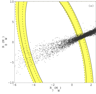
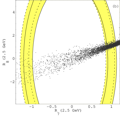
Figure 4.3: ${90\%\ \mathrm{C.L.}}$ bounds in the $[R_{7}(\mu),R_{8}(\mu)]$ plane following from the world average $B\rightarrow X_{s}\gamma$ branching ratio for $\mu=m_{W}$ (left-hand plot) and $\mu=2.5$ GeV (right-hand plot). Theoretical uncertainties are taken into account. The solid and dashed lines correspond to the $m_{c}=m_{c,pole}$ and $m_{c}=m_{c}^{\overline{MS}}(\mu_{b})$ cases respectively. The scatter points correspond to the expectation in MFV models (the ranges of the SUSY parameters are specified in the text) [20].

In order to produce bounds that can be compared with the model independent allowed regions plotted in Fig (4.4), it turns out that the surviving SUSY points can be divided to two sets [20]:

• For small $\tan\beta$, for which we again take $\tan\beta=2.3$, we find that the ratio $R_{7}$ remains positive, i.e. ${C_{7}}^{\rm eff}<0$, and lies within the experimentally allowed bounds from $B\rightarrow X_{s}\gamma$, and the corresponding bounds on the semileptonic coefficients are in the range $-0.2<C_{9}^{MFV}(\mu_{W})<0.4$ and $-1.0<C_{10}^{MFV}(\mu_{W})<0.7$.

• For large $\tan\beta$, taken to be 50, ${C_{7}}^{\rm eff}$ changes sign ($R_{7}<0$). The corresponding bounds on $C_{9}^{MFV}$ and $C_{10}^{MFV}$ tend to be in the range $-0.2<C_{9}^{MFV}(\mu_{W})<0.3$ and $-0.8<C_{10}^{MFV}(\mu_{W})<0.5$.

The above discussion applies to any supersymmetric model with flavour universal soft-breaking terms, such as mSUGRA MSSM and gauge-mediated supersymmetry breaking models. Beyond-the-SM flavour violations in such models are induced only via renormalization group running, and are tiny. Before ending this subsection, let us discuss the impact of $b\rightarrow s\gamma$ on MFV models in varying the MFV SUSY parameters:

• The strong correlation between the values of the Wilson coefficients $C_{7}$ and $C_{8}$, shown in Fig. 4.3. In fact, the SUSY contributions to the magnetic and chromo–magnetic coefficients differ only because of colour factors and loop-functions.

• The dependence of the charged Higgs contribution to magnetic coefficient at the scale $\mu_{b}$, can be seen from Fig. 12 in ref [20]. It turns out that with a specific scenario, it is possible to obtain lower bounds on some SUSY particles.

• The chargino contributions on $C_{7}(\mu_{b})$, show very strong consequences on the $b\rightarrow s\gamma$ transition as it has been shown in [20]. Assuming for instance $m_{\tilde{t}_{2}}=m_{\chi}=500\;{\hbox{GeV}}$ the chargino contributions (normalized to $(\sin\theta_{\tilde{t}}\tan\beta)$) is of order 0.2. If one then allows for larger values of the stop mixing angle and of $\tan\beta$, the contribution can easily violate the $b\rightarrow s\gamma$ constraint by more than one order of magnitude (e.g. for $\sin\theta_{\tilde{t}}=0.5$ and $\tan\beta=50$ one obtains something of order 6 that is orders of magnitude above the current limit) [20].

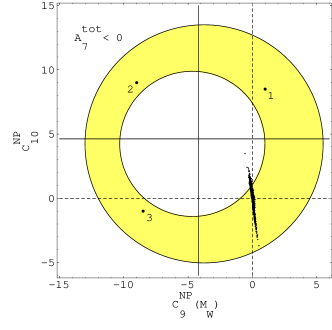
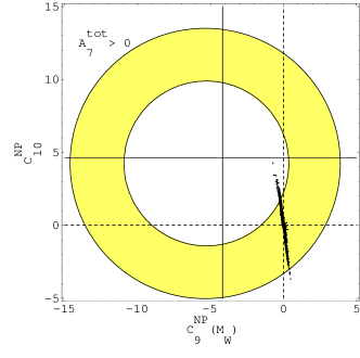
Figure 4.4: NNLO Case. Superposition of all the constraints. The plots correspond to the $A_{7}^{\rm tot}(2.5\;{\hbox{GeV}})<0$ and $A_{7}^{\rm tot}(2.5\;{\hbox{GeV}})>0$ case, respectively. The points are obtained by means of a scanning over the EMFV parameter space and requiring the experimental bound from $B\rightarrow X_{s}\gamma$ to be satisfied [20].

Up to this point we have been looking at the minimal case where all genuine sources of flavour changing transitions in the MSSM are attributed to the CKM matrix elements. However, an interesting question to ask is whether there might be other, non-universal scenarios, where new flavour changing transitions (other than the CKM mixing elements) could occur. A model which incorporates these features is the so-called Extended-MFV (EMFV) model [148], discussed in the following subsection.

4.5.3 The Extended-MFV model

The Extended-MFV (EMFV) model which is a generalization of the MFV-model using the language of minimal insertion approximation (MIA) [153] in a supersymmetric context. Its main assumption lies in the fact that new sources of flavour changing transitions other than the CKM mixing elements could occur.

EMFV-models are based on the heavy squarks and gluino assumption. Moreover, the charged Higgs and the lightest chargino and stop masses are required to be heavier than $100\;{\hbox{GeV}}$ in order to satisfy the lower bounds from direct searches. The rest of the SUSY spectrum is assumed to be almost degenerate and heavier than $1\;\textrm{TeV}$. The lightest stop is almost right-handed and the stop mixing angle (which parameterizes the amount of the left-handed stop $\tilde{t}_{L}$ present in the lighter mass eigenstate) turns out to be of order $\sim 10\%$; for definiteness we will take $|\theta_{\tilde{t}}|\leq\pi/10$.

The assumption of a heavy ($\geq 1$ TeV) gluino totally suppresses any possible gluino–mediated SUSY contribution to low energy observables. Note that even in the presence of a light gluino (i.e. $m_{\tilde{g}}\simeq O(300\;{\hbox{GeV}})$) these penguin diagrams remain suppressed due to the heavy down squarks present in the loop. On the other hand, the presence of only a single light squark mass eigenstate (out of twelve) has strong consequences due to the rich flavour structure which emerges from the squark mass matrices. Adopting the MIA-framework [153], all FC transitions which are not generated by the CKM mixing matrix are proportional to the properly normalized off-diagonal elements of the squark mass matrices:

$$(\delta_{ij})^{U,D}_{AB}\equiv{(M^{2}_{ij})^{{\scriptscriptstyle U},{\scriptscriptstyle D}}_{AB}\over M_{\tilde{q}_{i}}M_{\tilde{q}_{j}}}$$ (4.48)

where $i,j=1,2,3$ and $A,B=L,R$. In this approach, some remarks are in order:

• The only sizable contributions arise from the inserted mass insertions involving the light stop.

• All the other diagrams require necessarily a loop with at least two heavy ($\geq 1\;\textrm{TeV}$) squarks and are therefore automatically suppressed.

This leaves us with only two unsuppressed flavour changing sources other than the CKM matrix, namely the mixings $\tilde{u}_{L}-\tilde{t}_{2}$ (denoted by $\delta_{\tilde{u}_{L}\tilde{t}_{2}}$) and $\tilde{c}_{L}-\tilde{t}_{2}$ (denoted by $\delta_{\tilde{c}_{L}\tilde{t}_{2}}$). We note that $\delta_{\tilde{u}_{L}\tilde{t}_{2}}$ and $\delta_{\tilde{c}_{L}\tilde{t}_{2}}$ are mass insertions extracted from the up-squarks mass matrix after the diagonalization of the stop system and are therefore linear combinations of $(\delta_{13})^{U}_{LR}$, $(\delta_{13})^{U}_{LL}$ and of $(\delta_{23})^{U}_{LR}$, $(\delta_{23})^{U}_{LL}$, respectively. The insertions relevant to our discussion are normalized as follows:

$$\delta_{\tilde{u}(\tilde{c})_{L}\tilde{t}_{2}}\equiv{M^{2}_{\tilde{u}(\tilde{c})_{L}\tilde{t}_{2}}\over M_{\tilde{t}_{2}}M_{\tilde{q}}}{|V_{td(s)}|\over V_{td(s)}^{*}}\;.$$ (4.49)

The phenomenological impact of $\delta_{\tilde{t}_{2}\tilde{u}_{L}}$ has been studied in [148] and its impact on the $b\rightarrow s\gamma$ and $b\rightarrow s\ell^{+}\ell^{-}$ transitions is indeed negligible. Therefore, we are left with the MIA parameter $\delta_{\tilde{t}_{2}\tilde{c}_{L}}$ only. Thus, the SUSY parameter space that we have to deal with are the same as the MFV-model with MIA parameter $\delta_{\tilde{t}_{2}\tilde{c}_{L}}$. In order to explore the region in the $[C_{9}^{NP},C_{10}^{NP}]$ plane (where $C_{9,10}^{NP}$ are the sum of MFV and MI contributions) that is accessible to these models, one has to apply the $b\rightarrow s\gamma$ constraint on the EMFV parameter space, which are the same as the MFV-ones apart from $|\theta_{\tilde{t}}|\leq\pi/10$ and $|\delta_{\tilde{t}_{2}\tilde{c}_{L}}|\leq 1$. The surviving points are shown in Fig. 4.4 together with the model independent constraints. To get them, one has to use the integrated branching ratios to put constraints on the effective coefficients. This procedure allows multiple solutions, which can be disentangled from each other only with the help of both the dilepton mass spectrum and the forward-backward asymmetry. Only such measurements would allow us to determine the exact values and signs of the Wilson coefficients $C_{7}$, $C_{9}$ and $C_{10}$.

4.6 The ratios $R_{-}(s)$ and $R_{0}(s)$ as probes of New Physics in $B\rightarrow K^{*}\ell^{+}\ell^{-}$

In order to look for new physics in $B\rightarrow K^{*}\ell^{+}\ell^{-}$, we propose to study the ratios $R_{0}(s)$ and $R_{-}(s)$, introduced in the previous section. As well known, new physics can distort the dilepton invariant mass spectrum and the forward-backward asymmetry in a non-trivial way.

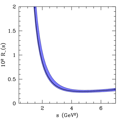
Figure 4.5: The Ratios $R_{-}(s)$ (left-hand plot) and $R_{0}(s)$ (right-hand plot) in the Standard Model with $R_{b}=0.094$, $\zeta_{SU(3)}=1.3$, $\xi^{(K^{*})}_{{\perp}}(0)=0.28$ and in SUGRA, with $(r_{7},\ r_{8})=(1.1,\ 1.4)$. The SM and the SUGRA contriburions are represented respectively by the shaded area and the solid curve. The shaded area depicts the theoretical uncertainty on $\zeta_{SU(3)}=1.3\pm 0.06$ and on $\xi^{(K^{*})}_{{\perp}}=0.28\pm 0.04$ [29].

To illustrate generic SUSY effects in ${B\rightarrow K^{*}\ell^{+}\ell^{-}}$, we note that the Wilson coefficients $C^{\bf eff}_{7}$, $C^{\bf eff}_{8}$, $C_{9}$ and $C_{10}$ receive additional contributions from the supersymmetric particles. We incorporate these effects by assuming that the ratios of the Wilson coefficients in these theories and the SM deviate from 1. These ratios for $k=7,8,9,10$ are defined as follows:

$$r_{k}(\mu)={C_{k}^{SUSY}\over C_{k}^{SM}}~{}.$$ (4.50)

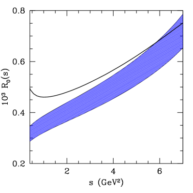
Figure 4.6: The Ratios $R_{-}(s)$ (left-hand plot) and $R_{0}(s)$ (right-hand plot) in the Standard Model with $R_{b}=0.094$, $\zeta_{SU(3)}=1.3$, $\xi^{(K^{*})}_{{\perp}}(0)=0.28$ and in SUGRA, with $(r_{7},\ r_{8})=(-1.2,\ -1)$. The SM and the SUGRA contributions are represented respectively by the shaded area and the solid curve. The shaded area depicts the theoretical uncertainty on $\zeta_{SU(3)}=1.3\pm 0.06$ and on $\xi^{(K^{*})}_{{\perp}}=0.28\pm 0.04$ [28].

They depend on the renormalization scale (except for $C_{10}$), for which we take $\mu=m_{b,pole}$. For the sake of illustration, we use representative values for the large-$\tan\beta$ SUGRA model, in which the ratios $r_{7}$ and $r_{8}$ actually keep or change their signs. The supersymmetric effects on the other two Wilson coefficients $C_{9}$ and $C_{10}$ are generally small in the SUGRA models, leaving $r_{9}$ and $r_{10}$ practically unchanged from their SM value. To be specific, we take the two allowed scenarios

$$r_{7}=-1.2,\ \ r_{8}=-1,\ \ \ r_{9}=1.03,\ \ r_{10}=1.0,$$ (4.51)

and

$$r_{7}=1.1,\ \ r_{8}=1.4,\ \ \ r_{9}=1.03,\ \ r_{10}=1.0.$$ (4.52)

In Figs. (3.27), (3.28), (4.5) and (4.6), we present a comparative study of the SM and SUGRA partial distribution for $H_{-}$ and $H_{0}$, respectively. In doing this, we also show the attendant theoretical uncertainties for the SM, worked out in the LEET approach [28]. For these distributions, we have used the form factors from [31] with the SU(3)-symmetry breaking parameter taken in the range $\zeta_{SU(3)}=1.3\pm 0.06$.

From Fig. (4.5) , where $r_{k}>0,~{}~{}(k=7,8,9,10)$, it is difficult to work out a signal of new physics from the SM picture. There is no surprise to be expected, due to the fact that in these scenario the corresponding ratio $r_{k}$ is approximatively one, which makes the SUGRA picture closer to the SM one. However, Fig. (4.6) with $(r_{7},\ r_{8})<0$ illustrate clearly that despite non-perturbative uncertainties, it is possible, in principle, in the low $s$ region to distinguish between the SM and a SUGRA-type models, provided the ratios $r_{k}$ differ sufficiently from 1.

4.7 Summary and Outlook

In this chapter we have presented a phenomenological profile of the semileptonic rare $B\rightarrow K^{*}\ell^{+}\ell^{-}$ decay in the context of supersymmetric theories. Considering the straightforward supersymmetrization version of the SM, the so-called MSSM, we have reviewed in details its contribution to the $b\rightarrow s\ell^{+}\ell^{-}$ process. We illustrate the constraints on the Wilson coefficients $C_{7}$, $C_{8}$, $C_{9}$ and $C_{10}$ appearing in the effective Hamiltonian formalism, that the current data on rare $B$ decays implies in the context of minimal flavour violating model and in more general scenarios admitting additional flavour changing mechanisms. Finally, incorporating these supersymmetric effects on the corresponding Wilson coefficients, we have shown their phenomenological impact on the ratios $R_{0}(s)$ and $R_{-}(s)$ as probes of new physics.

Our studies can be reported as follows [28] :

• We have shown within the MSSM framework the complete SUSY contributions to the $b\rightarrow s\ell^{+}\ell^{-}$ decay. Beyond the $W$-exchange in the SM, four other classes contribute to this process, namely the $Higgs$-exchange, $Chargino$-exchange, $gluino$-exchange and the $Neutralino$-ones.

• Using the current data constraints on rare $B$ decays, we have discussed their phenomenological impacts on the Wilson coefficients $C_{7}$, $C_{8}$, $C_{9}$ and $C_{10}$. It turns out that present experimental measurements leave considerable room for beyond-the-SM contributions , especially, to the allowed region in the $[C_{9},C_{10}]$ plane. However, in the SUGRA models they are practically unchanged from their SM value.

• In order to look for new physics in $B\rightarrow K^{*}\ell^{+}\ell^{-}$, we propose to study the ratios $R_{0}(s)$ and $R_{-}(s)$. For the sake of illustration, we use representative values for the large-$\tan\beta$ SUGRA model with two scenarios, namely $(r_{7},\ r_{8})<0$ and $(r_{7},\ r_{8})>0$ . We have noticed that despite non-perturbative uncertainties, it is possible when $(r_{7},\ r_{8})<0$ , in principle, in the low $s$ region to distinguish between the SM and a SUGRA-type models, provided the ratios $r_{k}$ differ sufficiently from 1.

Chapter 5 Summary & Future

While waiting for the completion of the second-generation experiments at hadron colliders, $\mathrm{BTeV}$ (Fermilab) and LHCb (CERN), $B$-physics is among the most active and promising fields in recent particle physics. Its importance lies in the deeper understanding of the Standard Model and particle physics in general. The futur investigation of $b$ decays (such as rare $B$-decays, two leptonic $B$-decays, $\cdots$ ) at the $B$-factories, namely BABAR and BELLE, and at hadron colliders will probe the flavour sector of the SM with unprecedented precision, and may be reveal new physics effects.

Rare $B$ decays involving flavour-changing-neutral-current (FCNC) transitions, such as $b\rightarrow s\gamma$ and $b\rightarrow s\ell^{+}\ell^{-}$, have received a lot of theoretical interest [154]. Especially, after the first measurements of the radiative decay $B\rightarrow X_{s}\gamma$ were reported by the CLEO collaboration [155] in 1995 and recently the first measurements of the semileptonic rare $B$-decays reported in the inclusive (exclusive) $B\rightarrow X_{s}(K,K^{*})\ell^{+}\ell^{-}$ by the BELLE collaboration [14] (BABAR collaboration [18]). With increased statistical power of experiments at the $B$-factories in the next several years, the decays discussed above and related rare $B$ decays will be measured very precisely. We summarize the projections for improvement in the experimental contributions to the precision of CKM matrix elements $V_{ub}$, $V_{cb}$ and $V_{ts}$ [156] in Table 5.1 while in Table 5.2 [156] the decay reach of the rare $B$-decays is given.

$V_{ij}$	Experimental	$\sigma~{}(\%)$	$\sigma~{}(\%)$	$\sigma~{}(\%)$
	Measurement	2001	2006	2011
		stat/sys	stat/sys	stat/sys
$V_{ub}$	${\mathcal{B}}(B\rightarrow\rho~{}\ell\nu_{\ell})$	$4.3/8$	$8.6/2.4$	$1.4/2.4$
	${\mathcal{B}}(B\rightarrow u~{}\ell\nu_{\ell})$	$3.4/16$	$4.0/2.4$	$2.8/2.4$
$V_{cb}$	${\mathcal{B}}(B\rightarrow D~{}\ell\nu_{\ell})$	$3.1/4$	$0.4/2$	$0.10/1$
	${\mathcal{B}}(B\rightarrow c~{}\ell\nu_{\ell})$	$2.5/2$	$0.3/1$	$0.07/0.5$
$V_{ts}$	$\Delta m_{s}$

Table 5.1: Projections for improvement in the experimental contributions to the precision of CKM matrix elements $V_{ub}$, $V_{cb}$ and $V_{ts}$ [156].

Within this thesis, we have reported an $O(\alpha_{s})$-improved analysis of the various helicity components in the decays $B\rightarrow K^{*}\ell^{+}\ell^{-}$ and $B\rightarrow\rho\ell\nu_{\ell}$, carried out in the context of the Large-Energy-Effective-Theory. Our studies can be summarized as follows [28, 29] :

• The underlying symmetries in the large energy limit lead to an enormous simplification as they reduce the number of independent form factors in these decays. The LEET-symmetries are broken by QCD corrections, and we have calculated the helicity components implementing the $O(\alpha_{s})$ corrections.

• The results presented here make use of the form factors calculated in the QCD sum rule approach. The LEET form factor $\xi_{\perp}^{(K^{*})}(0)$ is constrained by current data on $B\rightarrow K^{*}\gamma$.

• As the theoretical analysis is restricted to the lower part of the dilepton invariant mass region in $B\rightarrow K^{*}\ell^{+}\ell^{-}$, typically $s<8$ GeV², errors in this form factor are not expected to severely limit theoretical precision. This implies that distributions involving the $H_{-}(s)$ helicity component can be calculated reliably. Precise measurements of the two LEET form factors $\xi_{\perp}^{(\rho)}(s)$ and $\xi_{\parallel}^{(\rho)}(s)$ in the decays $B\rightarrow\rho\ell\nu_{\ell}$ can be used to largely reduce the residual model dependence.

• With the assumed form factors, we have worked out a number of single and double (Dalitz) distributions in $B\rightarrow\rho\ell\nu_{\ell}$, which need to be confronted with data.

• An analysis of the decays $B\rightarrow K^{*}\ell^{+}\ell^{-}$ is also carried out in the so-called transversity basis. We have compared the LEET-based amplitudes in this basis with the data currently available on $B\rightarrow K^{*}J/\psi(\rightarrow\ell^{+}\ell^{-})$ and find that the short-distance based transversity amplitudes are very similar to their long-distance counterparts.

• We also show the $O(\alpha_{s})$ effects on the forward-backward asymmetry, confirming essentially the earlier work of Beneke, Feldmann and Seidel [25].

• Combining the analysis of the decay modes $B\rightarrow K^{*}\ell^{+}\ell^{-}$ and $B\rightarrow\rho\ell\nu_{\ell}$, we show that the ratios of differential decay rates involving definite helicity states, $R_{-}(s)$ and $R_{0}(s)$, can be used for testing the SM precisely. We work out the dependence of these ratios on the CKM matrix elements $|V_{ub}|/|V_{ts}|$. We have also analyzed possible effects on these ratios from New Physics contributions, exemplified by representative values for the effective Wilson coefficients in SUGRA models.

The main thrust of this work lies, however, on showing that the currently prevailing theoretical uncertainties on the SM distributions in $B\rightarrow K^{*}\ell^{+}\ell^{-}$ can be largely reduced by using the LEET approach and data on $B\rightarrow K^{*}\gamma$ and $B\rightarrow\rho\ell\nu_{\ell}$ decays.

Finally, we remark that the current experimental limits on $B\rightarrow(X_{s},K,K^{*})\ell^{+}\ell^{-}$ decays [?–?] are already probing the SM-sensitivity. With the integrated luminosities over the next couple of years at the $B$-factories, the helicity analysis in $B\rightarrow\rho\ell\nu_{\ell}$ and $B\rightarrow K^{*}\ell^{+}\ell^{-}$ decays presented here can be carried out experimentally. This work will help the search for flavour changing neutral current $B\rightarrow K^{*}\ell^{+}\ell^{-}$ and in particular, will contribute to precise determinations of the LEET form factors, and the CKM matrix elements $|V_{ub}|/|V_{ts}|$ using as well the $B\rightarrow\rho\ell\nu_{\ell}$ decay in forthcoming $B$-facilities.

		Hadron Collider Experiments			$e^{+}e^{-}$ $B$ Factories
Decay Mode	Branching	CDF	BTeV	ATLAS	BaBar	Super-
	Fractions	D0	LHCb	CMS	Belle	BaBar
		$(2\,\mathrm{fb}^{-1})$	$(10^{7}\,\mathrm{s})$	$(1\,\mathrm{Year})$	$(0.5\,\mathrm{ab}^{-1})$	$(10\,\mathrm{ab}^{-1})$
$B\rightarrow X_{s}\gamma$	$(3.3\pm 0.3)$				11K	220K
	$\times 10^{-4}$				1.7K	34K
					$(\mathrm{B~{}Tagged})$	$(\mathrm{B~{}Tagged})$
$B\rightarrow K^{*}\gamma$	$5\times 10^{-6}$	170	25K		6K	120K
$B\rightarrow\rho(\omega)\gamma$	$2\times 10^{-6}$				300	6K
$B\rightarrow X_{s}\mu^{+}\mu^{-}$	$(6.0\pm 1.5)\times 10^{-6}$		3.6K		300	6K
$B\rightarrow X_{s}e^{+}e^{-}$					350	7K
$B\rightarrow K^{*}\mu^{+}\mu^{-}$	$(2\pm 1)\times 10^{-6}$	60-150	2.2K/4.5K	665/4.2K	120	2.4K
$B\rightarrow K^{*}e^{+}e^{-}$					150	3K

Table 5.2: Decay reach of $B$ experiments for rare decays [156].

Appendix A Generalities

A.1 Input Parameters

$M_{W}$	$80.4$ GeV	$f_{B}$	$200\pm 20$ MeV
$\hat{m}_{t}(\hat{m}_{t})$	$167\pm 5$ GeV	$f_{K^{*},\parallel}$	$225\pm 30$ MeV
$m_{b,pole}(2\,\mbox{GeV})$	$4.6\pm 0.1$ GeV	$f_{K^{*},\perp}(1\,\mbox{GeV})$	$185\pm 10$ MeV
$m_{c}$	$1.4\pm 0.2$ GeV	$f_{\rho}$ (1 GeV)	$198\pm 7$ MeV
$\alpha_{em}$	$1/137$	$\lambda_{B,+}^{-1}$	$(3\pm 1)$ GeV
$\tau_{B}$	1.65 ps	$a_{1}(K^{*})_{\perp,\,\parallel}$	$0.2\pm 0.1$
$|V_{ts}^{*}V_{tb}|$	$0.041\pm 0.003$	$a_{2}(K^{*})_{\perp,\,\parallel}$	$0.05\pm 0.1$
$R_{b}=|V_{ub}|/|V_{ts}^{*}V_{tb}|$	$0.094\pm 0.014$	$\xi^{(K^{*})}_{\perp}(0)$	$0.28\pm 0.04$
$\Lambda_{\rm QCD}^{(n_{f}=5)}$	$220\pm 40$ MeV	$\xi^{(\rho)}_{\perp}(0)$	$0.22\pm 0.04$
$\langle\ell_{+}^{-1}\rangle^{(\rho)}_{+}$	$0.3\pm 0.2$  $(GeV)^{-1}$	$\langle\overline{u}^{-1}\rangle^{(\rho)}_{||}$	3.48

Table A.1: Input parameters and their uncertainties used in the calculations of the decay rates for $B\rightarrow K^{*}\ell^{+}\ell^{-}$ and $B\rightarrow\rho\ell\nu_{\ell}$ in the LEET approach.

A.2 QCD

The QCD Lagrangian reads in covariant gauge [161] ($A^{a}_{\mu}$: gluon field)

$${\cal L}_{QCD}=\sum_{q=u,d,s,c,b,t}\overline{q}(iD\hskip-5.0pt/-m_{q})q-\frac{1}{4}G_{\mu\nu}^{a}G^{a\,\mu\nu}+{\cal L}_{fix}+{\cal L}_{ghosts}\;,$$ (A.1)

where the gauge fixing term and the one for ghosts $c^{a},\overline{c}^{a}$ are given as

$${\cal L}_{fix} = -\frac{1}{2\xi}(\partial\cdot A^{a})^{2}\;,$$ (A.2)

$${\cal L}_{ghosts} = \overline{c}^{a}\partial\cdot D^{ab}c^{b}\;.$$ (A.3)

The chromomagnetic field strength tensor and covariant derivative are written as

$$G^{a}_{\mu\nu} = \partial_{\mu}A_{\nu}^{a}-\partial_{\nu}A_{\mu}^{a}+gf^{axy}A_{\mu}^{x}A_{\nu}^{y}\;,$$ (A.4)

$$D_{\mu} = \partial_{\mu}-igT^{x}A_{\mu}^{x}\;,$$ (A.5)

$$D_{\mu}^{ab} = \delta^{ab}\partial_{\mu}-gf^{abx}A_{\mu}^{x}\;,$$ (A.6)

where $f^{abx}$ are the structure constants of $SU(3)$, defined by

$$[T^{a},T^{b}]=if^{abx}T^{x}\;.$$ (A.7)

We have the identities

$$[D_{\mu},D_{\nu}] = -igT^{x}G^{x}_{\mu\nu}\;,$$ (A.8)

$$D^{ax}_{\mu}D^{xb}_{\nu}-D^{ax}_{\nu}D^{xb}_{\mu} = -gf^{abx}G^{x}_{\mu\nu}\;.$$ (A.9)

Often the abbreviation is used

$$G_{\mu\nu}=G_{\mu\nu}^{a}T^{a}\;.$$ (A.10)

$T^{a},\,a=1,\dots,8$ are the generators of QCD. They are related to the Gell-Mann $(3\times 3)$ matrices $\lambda^{a}$ through $T^{a}=\frac{\lambda^{a}}{2}$. The $T^{a}$ obey the following relations ($i,j,k=1,2,3$)

$$Sp(T_{a}) = 0\;,$$ (A.11)

$$Sp(T_{a}T_{b}) = \delta_{ab}/2\;,$$ (A.12)

$$T^{a}_{ij}T^{a}_{kl} = -\frac{1}{2N_{c}}\delta_{ij}\delta_{kl}+\frac{1}{2}\delta_{ik}\delta_{jl}\;,$$ (A.13)

$$T^{a}_{il}T^{a}_{lk} = \delta_{ik}C_{F}\;,$$ (A.14)

with the invariant $C_{F}$ in an arbitrary $SU(N_{c})$ given as

$$C_{F}=\frac{N_{c}^{2}-1}{2N_{c}}\;\;(=\frac{4}{3}\;\;{\mbox{for}}\;N_{c}=3)\;.$$ (A.15)

The coefficients of the QCD beta function (see Eq. (2.29)) are written as:

$$\beta_{0} = \frac{11N_{c}-2N_{f}}{3}\;,$$ (A.16)

$$\beta_{1} = \frac{34N_{c}^{2}-10N_{c}N_{f}-6C_{F}N_{f}}{3}\;.$$ (A.17)

Here, $N_{c}$ denotes the number of colours ($N_{c}=3$ for QCD) and $N_{f}$ denotes the number of active flavours ($N_{f}=5$ for the effective Hamiltonian theory relevant for $b$ decays).

A.3 Feynman Rules

The covariant derivative consistent with our definition of the operator basis and the corresponding Wilson coefficients given in section 2.2 is [53]

$$D_{\mu}\equiv\partial_{\mu}+igT^{a}A_{\mu}^{a}+ieQA_{\mu}\;,$$ (A.18)

where $A^{a}_{\mu},A-\mu$ denote the polarization four-vectors of the gluon, photon respectively. Note that the sign convention of the strong coupling here is opposite to the usual one appearing in QCD text books [161, 162] given in Eq. (A.5), but can be made consistent with the substitution $g\rightarrow-g$. The Feynman rules consistent with eq. (A.18) are given here with boson propagators in Feynman gauge. In a general gauge with gauge parameter $\xi$ they are written as:

$$-i\frac{g_{\mu\nu}+(\xi-1)k_{\mu}k_{\nu}/(k^{2}+i\epsilon)}{k^{2}+i\epsilon}\;,$$ (A.19)

with $\xi=1,0$ corresponding to Feynman, Landau gauge, respectively. The Feynman rules are :

complemented by the rules :

• evaluate fermion lines against the momentum flow

• add a $(-1)$ for a closed fermion loop and perform the trace over the string of $\gamma$ matrices

The rule for an $O_{7}$ operator insertion is, using $\partial_{\mu}=iq_{\mu}$ for an out going photon and further $\epsilon\cdot q=0$ for a real photon, and $F^{\mu\nu}=\partial^{\mu}A^{\nu}-\partial^{\nu}A^{\mu}$,

$$\sigma F=\sigma_{\mu\nu}F^{\mu\nu}=i[\partial\hskip-5.0pt/,A\hskip-5.0pt/]=2\gamma_{\mu}q\hskip-5.0pt/\epsilon^{\mu}\;.$$ (A.20)

The Fierz transformation in $d=4$ dimensions is defined as:

$$(\overline{q}_{1}\gamma_{\mu}Lq_{2})(\overline{q}_{3}\gamma_{\mu}Lq_{4}) = +(\overline{q}_{1}\gamma_{\mu}Lq_{4})(\overline{q}_{3}\gamma_{\mu}Lq_{2})\;,$$ (A.21)

$$(\overline{q}_{1}\gamma_{\mu}L(R)q_{2})(\overline{q}_{3}\gamma_{\mu}R(L)q_{4}) = (-2)(\overline{q}_{1}R(L)q_{4})(\overline{q}_{3}L(R)q_{2})\;.$$ (A.22)

A.4 Utilities

A variety of tools for 1-loop calculations is collected in the appendix of ref. [162].
Distributions :

$$\delta(x) = \frac{1}{2\pi}\int_{\mbox{R}}dqe^{iqx}dq\;,$$ (A.23)

$$\theta(x) = \lim_{\epsilon\rightarrow 0}\frac{-i}{2\pi}\int_{\mbox{R}}dq\frac{e^{iqx}}{q-i\epsilon}dq\;,$$ (A.24)

$$\frac{d\theta}{dx}(x) = \delta(x)\;.$$ (A.25)

Geometrical series :

$$\frac{1}{1\pm x}=1\mp x+x^{2}+\sum_{n=3}^{\infty}(\mp x)^{n}\;.$$ (A.26)

Special Functions useful for loops
Poly-logarithms :

$$Li_{n}(z) = \sum_{k=1}^{\infty}\frac{z^{k}}{k^{n}};\;|z|<1\;,$$ (A.27)

$$Li_{2}(z) = -\int_{0}^{z}\frac{dt}{t}\ln(1-t)\;.$$ (A.28)

Spence function :

$$Sp(z) \equiv Li_{2}(z)=-\int_{0}^{1}\frac{dt}{t}\ln(1-zt)\;,$$ (A.29)

$$Sp(0) = 0\;\;,\;\;Sp(1)=\frac{\pi^{2}}{6}\;\;,\;\;Sp(-1)=\frac{\pi^{2}}{12}\;\;,$$ (A.30)

$$Sp(z) = -Sp(1-z)+\frac{\pi^{2}}{6}-\ln(z)\ln(1-z)\;,$$ (A.31)

$$Sp(z) = -Sp(\frac{1}{z})-\frac{\pi^{2}}{6}-\frac{1}{2}\ln^{2}(-z)\;.$$ (A.32)

Useful identities for loops:

$$\arctan(z)=\frac{1}{2i}\ln\frac{1+iz}{1-iz}\;,~{}~{}{\mbox{arctanh}}(z)=\frac{1}{2}\ln\frac{1+z}{1-z}\;.$$ (A.33)

Phase space element, $d^{3}\vec{p}=|\vec{p}|^{2}~{}d|\vec{p}|~{}d\cos{\theta}~{}d\phi\;,\cos{\theta}\in[-1,+1]\;,\phi\in[0,2\pi[$.

$$\frac{d^{3}\vec{p}}{2E}=\int d^{4}p~{}\delta(p^{2}-m^{2})~{}\theta(E)\;\;;~{}~{}E=\sqrt{{\vec{p}}^{2}+m^{2}}\;.$$ (A.34)

Dirac algebra identities, for more see ref. [163], especially the appendix.

$$\{\gamma_{\mu},\gamma_{\nu}\}=2g_{\mu\nu}\;,~{}~{}\sigma_{\mu\nu}=\frac{i}{2}[\gamma_{\mu},\gamma_{\nu}]\;,~{}~{}\gamma_{\mu}\gamma_{\nu}=g_{\mu\nu}-i\sigma_{\mu\nu}\;.$$ (A.35)

A useful tool within this context is the TRACER routine [164] running under the symbolic algebra program mathematica.

Chiral projectors $L(R)\equiv(1\mp\gamma_{5})/2$:

$$\gamma_{5}^{2} = 1\;,~{}~{}\gamma_{5}^{\dagger}=\gamma_{5}\;,$$ (A.36)

$$(L(R))^{2} = L(R)\;,~{}~{}LR=RL=0\;,~{}~{}(L(R))^{\dagger}=L(R)\;.$$ (A.37)

Further we have

$$\gamma_{0}^{2} = 1\;,~{}~{}\gamma_{0}^{\dagger}=\gamma_{0}\;.$$ (A.38)

Fermion fields :

$$\overline{\psi} \equiv \psi^{\dagger}\gamma_{0}=(\psi^{*})^{T}\gamma_{0}\;,~{}~{}\psi_{L(R)}\equiv L(R)\psi\;,$$

$$\overline{\psi_{L(R)}} = \overline{L(R)\psi}=(L(R)\psi)^{\dagger}\gamma_{0}=\psi^{\dagger}(L(R))^{\dagger}\gamma_{0}=\psi^{\dagger}\gamma_{0}R(L)=\overline{\psi}R(L)\;.$$ (A.39)

Appendix B The large energy expansion

B.1 Feynman Rules in the Large Energy Limit of QCD

In the hadron limit of an infinitely heavy meson $M$ with mass $m_{M}\rightarrow\infty$ and large energy for the final one $E_{P(V)}\rightarrow\infty$, the QCD Lagrangian defined in (A.1) is just:

$${\mathcal{L}}_{\rm QCD}={\mathcal{L}}_{\rm LEET}+{\cal O}(1/E)\;,$$ (B.1)

where the effective Lagrangian is given by

$${\mathcal{L}}_{\rm LEET} = \overline{q}_{n}\,\frac{n\hskip-5.0pt/_{+}}{2}\,in_{-}\cdot D\,q_{n}\;.$$ (B.2)

where $q_{n}(x)=e^{iE_{q}n_{-}\cdot x}\,\frac{n\hskip-3.5pt/_{-}n\hskip-3.5pt/_{+}}{4}\,q(x)$ are the large components of the light quark spinor field. The $n_{+}=2v-n_{-}$ is a light-like vector with $n_{+}\cdot n_{-}=2$ and $E_{q}\approx E$ is the energy of the light quark. Here $v$ and $n$ denote respectively the four-velocity ($v^{2}=1$) of the heavy quark $Q$ with momentum $p_{Q}=m_{Q}v+k$ and the four light-like vector ($n_{-}^{2}=0$) parallel to the the light quark $p_{q}=En_{-}+k^{\prime}$, where the small residual momentum $k$ (and $k^{\prime}$ )of order $\Lambda_{QCD}$.

It follows immediately, the Feynman rules of the LEET formalism:

where the light quark $q$ is represented by a double line.

B.2 The Factorizabe corrections $\Delta F_{i}$

We give here the ${\cal O}(\alpha_{s})$- factorizable corrections to the LEET form factors (defined in Eqs. (2.68)-(2.77)). We now present the result for the hard scattering correction to $B\rightarrow P$ form factors, as defined by $\Delta f_{+,0,T}$ in Eqs. (2.68), (2.70). The renormalisation convention implies $\Delta f_{+}\equiv 0$ by definition. Thus, they are then given by [63]

$$\Delta f_{+} = 0,$$ (B.3)

$$\Delta f_{0} = \frac{m_{B}-2E_{P}}{2E_{P}}\,\Delta F_{P},$$ (B.4)

$$\Delta f_{T} = -\frac{m_{B}+m_{P}}{2E_{P}}\,\Delta F_{P},$$ (B.5)

with the quantity

$$\Delta F_{P} = \frac{8\pi^{2}f_{B}f_{P}}{N_{C}m_{B}}\,\langle l_{+}^{-1}\rangle_{+}\,\langle\overline{u}^{-1}\rangle_{P},$$ (B.6)

is defined in terms of moment of the leading twist distribution amplitude (as usual $\overline{u}=1-u$)

$$\langle\overline{u}^{-1}\rangle_{P}=\int du\frac{\phi(u)}{\overline{u}}.$$ (B.7)

For the $B$ meson, the quantity $\langle l_{+}^{-1}\rangle_{+}$ reads

$$\langle l_{+}^{-1}\rangle_{+}=\int dl_{+}\frac{\phi^{B}_{+}(l_{+})}{l_{+}}.$$ (B.8)

Note that $\Delta f_{0}$ vanishes at $s=0$ ($E_{P}=m_{B}/2$) as required on general grounds. Following the renormalisation convention, the hard correction to the other $B\rightarrow V$ form factors, defined in Eqs. (2.71)-(2.77), reads [63]

$$\Delta A_{1} = \Delta V=0,$$

$$\Delta A_{2} = \frac{m_{V}}{E_{V}}\,\frac{m_{B}}{m_{B}-m_{V}}\,\frac{m_{B}(m_{B}-2E_{V})}{4E_{V}^{2}}\,\Delta F_{\parallel}\ ,$$ (B.9)

$$\Delta T_{1} = \frac{m_{B}}{4E_{V}}\,\Delta F_{\perp},$$

$$\Delta T_{2} = \frac{1}{2}\,\Delta F_{\perp},$$

$$\Delta T_{3} = \frac{m_{B}}{4E_{V}}\,\Delta F_{\perp}+\frac{m_{V}}{E_{V}}\,\left(\frac{m_{B}}{2E_{V}}\right)^{2}\,\Delta F_{\parallel}.$$ (B.10)

We introduce the quantities

$$\Delta F_{\parallel} = \frac{8\pi^{2}f_{B}f_{V}}{N_{C}m_{B}}\,\langle l_{+}^{-1}\rangle_{+}\,\langle\overline{u}^{-1}\rangle_{\parallel},$$ (B.11)

$$\Delta F_{\perp} = \frac{8\pi^{2}f_{B}f_{\perp}}{N_{C}m_{B}}\,\langle l_{+}^{-1}\rangle_{+}\,\langle\overline{u}^{-1}\rangle_{\perp},$$ (B.12)

where the two terms, namely $\langle\overline{u}^{-1}\rangle_{\parallel}$ and $\langle\overline{u}^{-1}\rangle_{\perp}$ are given by

$$\langle\overline{u}^{-1}\rangle_{\parallel}=\int du\,\phi_{\parallel}(u)/\overline{u},$$ (B.13)

and

$$\langle\overline{u}^{-1}\rangle_{\perp}=\int du\,\phi_{\perp}(u)/\overline{u}.$$ (B.14)

B.3 The Functions $F_{i}^{(j)}$

In this appendix we list the functions $F_{8}^{(7,9)}$, $F_{1}^{(9)}$ and $F_{2}^{(7,9)}$ (defined in Eqs. (3.65) and (3.66)), representing the power correction to the matrix elements of the operators ${\cal O}_{8}$, ${\cal O}_{1}$ and ${\cal O}_{2}$ respectively. The corrected one loop matrix elements of ${\cal O}_{8}$ read [22]:

$$F_{8}^{(7)} = -\frac{32}{9}\,\ln\frac{\mu}{m_{b}}-\frac{8}{9}\,\frac{\tilde{s}}{1-\tilde{s}}\,\ln\tilde{s}-\frac{8}{9}\,i\pi-\frac{4}{9}\,\frac{11-16\tilde{s}+8\tilde{s}^{2}}{(1-\tilde{s})^{2}}$$ (B.16)

$$\quad+\frac{4}{9}\,\frac{1}{(1-\tilde{s})^{3}}\,\left[(9\tilde{s}-5\tilde{s}^{2}+2\tilde{s}^{3})\,B_{0}(\tilde{s})-(4+2\tilde{s})\,C_{0}(\tilde{s})\right],$$

and

$$F_{8}^{(9)} = \frac{16}{9}\,\frac{1}{1-\tilde{s}}\,\ln\tilde{s}+\frac{8}{9}\,\frac{5-2\tilde{s}}{(1-\tilde{s})^{2}}-\frac{8}{9}\,\frac{4-\tilde{s}}{(1-\tilde{s})^{3}}\left[(1+\tilde{s})\,B_{0}(\tilde{s})-2\,C_{0}(\tilde{s})\right],$$ (B.17)

where $\tilde{s}=s/m_{b}^{2}$, $B_{0}(\tilde{s})=B_{0}(q^{2},m_{b}^{2})$ is given in (3.57), and the integral

$$C_{0}(\tilde{s}) = \int_{0}^{1}dx\,\frac{1}{x\,(1-\tilde{s})+1}\,\ln\frac{x^{2}}{1-x\,(1-x)\,\tilde{s}}$$ (B.18)

can be expressed in terms of dilogarithms. The corresponding power correction to the matrix elements of the operators ${\cal O}_{1}$ and ${\cal O}_{2}$ are given respectively (using $L_{\mu}=\ln(\mu/m_{b})$, $L_{s}=\ln(\tilde{s})$ and $\tilde{m}_{c}=m_{c}/m_{b}$ ) as [22]:

$${}F_{1}^{(9)} = \left(-{{\frac{1424}{729}}}+{{\frac{16}{243}}}\,i\pi+{{\frac{64}{27}}}\,{L_{c}}\right){L_{\mu}}-{{\frac{16}{243}}}\,{L_{\mu}}\,{L_{s}}+\left({{\frac{16}{1215}}}-{{\frac{32}{135}}}\,{{\tilde{m}_{c}}}^{-2}\right){L_{\mu}}\,{\tilde{s}}$$ (B.19)

$$+ \left({{\frac{4}{2835}}}-{{\frac{8}{315}}}\,{{\tilde{m}_{c}}}^{-4}\right){L_{\mu}}\,{{\tilde{s}}}^{2}+\left({{\frac{16}{76545}}}-{{\frac{32}{8505}}}\,{{\tilde{m}_{c}}}^{-6}\right){L_{\mu}}\,{{\tilde{s}}}^{3}$$

$$- {{\frac{256}{243}}}\,{{L_{\mu}}}^{2}+f_{1}^{(9)}\,,$$

	$\tilde{m}_{c}=0.27$			$\tilde{m}_{c}=0.29$			$\tilde{m}_{c}=0.31$
$k_{1}^{(9)}(0,0)$	$-12.327$	$+$	$0.13512\,i$	$-11.973$	$+$	$0.16371\,i$	$-11.65$	$+$	$0.18223\,i$
$k_{1}^{(9)}(0,1)$	$-0.080505$	$-$	$0.067181\,i$	$-0.081271$	$-$	$0.059691\,i$	$-0.080959$	$-$	$0.051864\,i$
$k_{1}^{(9)}(1,0)$	$-33.015$	$-$	$0.42492\,i$	$-28.432$	$-$	$0.25044\,i$	$-24.709$	$-$	$0.13474\,i$
$k_{1}^{(9)}(1,1)$	$-0.041008$	$+$	$0.0078685\,i$	$-0.040243$	$+$	$0.016442\,i$	$-0.036585$	$+$	$0.024753\,i$
$k_{1}^{(9)}(2,0)$	$-76.2$	$-$	$1.5067\,i$	$-57.114$	$-$	$0.86486\,i$	$-43.588$	$-$	$0.4738\,i$
$k_{1}^{(9)}(2,1)$	$-0.042685$	$+$	$0.015754\,i$	$-0.035191$	$+$	$0.027909\,i$	$-0.021692$	$+$	$0.036925\,i$
$k_{1}^{(9)}(3,0)$	$-197.81$	$-$	$4.6389\,i$	$-128.8$	$-$	$2.5243\,i$	$-86.22$	$-$	$1.3542\,i$
$k_{1}^{(9)}(3,1)$	$-0.039021$	$+$	$0.039384\,i$	$-0.017587$	$+$	$0.050639\,i$	$0.013282$	$+$	$0.052023\,i$

Table B.1: Coefficients in the decomposition of $f_{1}^{(9)}$ for three values of $\tilde{m}_{c}$ [22].

	$\tilde{m}_{c}=0.27$			$\tilde{m}_{c}=0.29$			$\tilde{m}_{c}=0.31$
$k_{2}^{(9)}(0,0)$	$7.9938$	$-$	$0.81071\,i$	$6.6338$	$-$	$0.98225\,i$	$5.4082$	$-$	$1.0934\,i$
$k_{2}^{(9)}(0,1)$	$0.48303$	$+$	$0.40309\,i$	$0.48763$	$+$	$0.35815\,i$	$0.48576$	$+$	$0.31119\,i$
$k_{2}^{(9)}(1,0)$	$5.1651$	$+$	$2.5495\,i$	$3.3585$	$+$	$1.5026\,i$	$1.9061$	$+$	$0.80843\,i$
$k_{2}^{(9)}(1,1)$	$0.24605$	$-$	$0.047211\,i$	$0.24146$	$-$	$0.098649\,i$	$0.21951$	$-$	$0.14852\,i$
$k_{2}^{(9)}(2,0)$	$-0.45653$	$+$	$9.0402\,i$	$-1.1906$	$+$	$5.1892\,i$	$-1.8286$	$+$	$2.8428\,i$
$k_{2}^{(9)}(2,1)$	$0.25611$	$-$	$0.094525\,i$	$0.21115$	$-$	$0.16745\,i$	$0.13015$	$-$	$0.22155\,i$
$k_{2}^{(9)}(3,0)$	$-25.981$	$+$	$27.833\,i$	$-17.12$	$+$	$15.146\,i$	$-12.113$	$+$	$8.1251\,i$
$k_{2}^{(9)}(3,1)$	$0.23413$	$-$	$0.2363\,i$	$0.10552$	$-$	$0.30383\,i$	$-0.079692$	$-$	$0.31214\,i$
$k_{2}^{(7)}(0,0)$	$4.3477$	$+$	$0.56054\,i$	$4.0915$	$+$	$0.44999\,i$	$3.8367$	$+$	$0.3531\,i$
$k_{2}^{(7)}(0,1)$		0			0			0
$k_{2}^{(7)}(1,0)$	$1.5694$	$+$	$0.9005\,i$	$1.4361$	$+$	$0.73732\,i$	$1.3098$	$+$	$0.60185\,i$
$k_{2}^{(7)}(1,1)$	$0.0010623$	$-$	$0.12324\,i$	$-0.016454$	$-$	$0.11806\,i$	$-0.031936$	$-$	$0.10981\,i$
$k_{2}^{(7)}(2,0)$	$-0.14311$	$+$	$1.2188\,i$	$0.011133$	$+$	$1.05\,i$	$0.13507$	$+$	$0.89014\,i$
$k_{2}^{(7)}(2,1)$	$-0.12196$	$-$	$0.099636\,i$	$-0.13718$	$-$	$0.068733\,i$	$-0.14169$	$-$	$0.035553\,i$
$k_{2}^{(7)}(3,0)$	$-2.5739$	$+$	$0.59521\,i$	$-1.6949$	$+$	$0.76698\,i$	$-1.0271$	$+$	$0.77168\,i$
$k_{2}^{(7)}(3,1)$	$-0.18904$	$-$	$0.0025554\,i$	$-0.17416$	$+$	$0.049359\,i$	$-0.13592$	$+$	$0.093\,i$

Table B.2: Coefficients in the decomposition of $f_{2}^{(9)}$ and $f_{2}^{(7)}$ for three values of $\tilde{m}_{c}$ [22].

and

$${}F_{2}^{(9)} = \left({{\frac{256}{243}}}-{{\frac{32}{81}}}\,i\pi-{{\frac{128}{9}}}\,{L_{c}}\right){L_{\mu}}+{{\frac{32}{81}}}\,{L_{\mu}}\,{L_{s}}+\left(-{{\frac{32}{405}}}+{{\frac{64}{45}}}\,{{\tilde{m}_{c}}}^{-2}\right){L_{\mu}}\,{\tilde{s}}$$ (B.20)

$$+ \left(-{{\frac{8}{945}}}+{{\frac{16}{105}}}\,{{\tilde{m}_{c}}}^{-4}\right){L_{\mu}}\,{{\tilde{s}}}^{2}+\left(-{{\frac{32}{25515}}}+{{\frac{64}{2835}}}\,{{\tilde{m}_{c}}}^{-6}\right){L_{\mu}}\,{{\tilde{s}}}^{3}$$

$$+ {{\frac{512}{81}}}\,{{L_{\mu}}}^{2}+f_{2}^{(9)}\,,$$

$${}F_{2}^{(7)} = {{\frac{416}{81}}}\,{L_{\mu}}+f_{2}^{(7)}\,.$$ (B.21)

The analytic results for $f_{1}^{(9)}$, $f_{1}^{(7)}$, $f_{2}^{(9)}$, and $f_{2}^{(7)}$ (expanded up to $\tilde{s}^{3}$ and $(\tilde{m}_{c}^{2})^{3}$) are rather lengthy. The formulas become relatively short, however, if we give the charm quark mass dependence in numerical form (for the characteristic values of $\tilde{m}_{c}$=0.27, 0.29 and 0.31).

We write the functions $f_{a}^{(b)}$ as

$$f_{a}^{(b)}=\sum_{i,j}\,k_{a}^{(b)}(i,j)\,\hat{s}^{i}\,L_{s}^{j}\quad\quad\quad(a=1,2;\,b=7,9;\,i=0,...,3;\,j=0,1).$$ (B.22)

The numerical values for the quantities $k_{a}^{(b)}(i,j)$ are given in Tables (B.2) and (B.2).

Appendix C $B\rightarrow K^{*}\ell^{+}\ell^{-}$ in SUSY

C.1 The functions $f_{i}(x)$

In this appendix we give the various one-loop integral functions, namely $f_{i}(x)$ $(i=1,\cdots,8)$, which appear within the MSSM contributions to the magnetic dipole moment and to the semileptonic coefficients. They are given respectively by [135]:

$$f_{1}(x) = {-7+5x+8x^{2}\over 6(1-x)^{3}}-{2x-3x^{2}\over(1-x)^{4}}\log x,$$ (C.1)

$$f_{2}(x) = {3x-5x^{2}\over 2(1-x)^{2}}+{2x-3x^{2}\over(1-x)^{3}}\log x,$$ (C.2)

$$f_{3}(x) = {2+5x-x^{2}\over 6(1-x)^{3}}+{x\over(1-x)^{4}}\log x,$$ (C.3)

$$f_{4}(x) = {1+x\over 2(1-x)^{2}}+{x\over(1-x)^{3}}\log x,$$ (C.4)

$$f_{5}(x) = {x\over 1-x}+{x\over(1-x)^{2}}\log x,$$ (C.5)

$$f_{6}(x) = {38x-79x^{2}+47x^{3}\over 6(1-x)^{3}}+{4x-6x^{2}+3x^{4}\over(1-x)^{4}}\log x,$$ (C.6)

$$f_{7}(x) = {52-101x+43x^{2}\over 6(1-x)^{3}}+{6-9x+2x^{3}\over(1-x)^{4}}\log x,$$ (C.7)

$$f_{8}(x) = {2-7x+11x^{2}\over(1-x)^{3}}+{6x^{3}\over(1-x)^{4}}\log x.$$ (C.8)

C.2 The Auxiliary Functions $c_{i}(m_{1}^{2},m_{2}^{2},m_{3}^{2})$, $d_{i}(m_{1}^{2},m_{2}^{2},m_{3}^{2},m_{4}^{2})$

The various auxiliary functions $c_{i}(m_{1}^{2},m_{2}^{2},m_{3}^{2})$ and $d_{i}(m_{1}^{2},m_{2}^{2},m_{3}^{2},m_{4}^{2})$ are listed below [135]:

$$c_{0}(m_{1}^{2},m_{2}^{2},m_{3}^{2}) = -\Bigl{[}{m_{1}^{2}\,\displaystyle{\log{m_{1}^{2}\over\mu^{2}}}\over(m_{1}^{2}-m_{2}^{2})(m_{1}^{2}-m_{3}^{2})}+(m_{1}\leftrightarrow m_{2})+(m_{1}\leftrightarrow m_{3})\Bigr{]},$$ (C.9)

$$c_{2}(m_{1}^{2},m_{2}^{2},m_{3}^{2}) = -{1\over 4}\Bigl{[}{m_{1}^{2}\,\displaystyle{\log{m_{1}^{4}\over\mu^{2}}}\over(m_{1}^{2}-m_{2}^{2})(m_{1}^{2}-m_{3}^{2})}+(m_{1}\leftrightarrow m_{2})+(m_{1}\leftrightarrow m_{3})\Bigr{]}$$ (C.10)

$$+{3\over 8},$$

$$d_{0}(m_{1}^{2},m_{2}^{2},m_{3}^{2},m_{4}^{2}) = -\Bigl{[}{m_{1}^{2}\,\displaystyle{\log{m_{1}^{2}\over\mu^{2}}}\over(m_{1}^{2}-m_{2}^{2})(m_{1}^{2}-m_{3}^{2})(m_{1}^{2}-m_{4}^{2})}+(m_{1}\leftrightarrow m_{2})$$ (C.11)

$$+(m_{1}\leftrightarrow m_{3})+(m_{1}\leftrightarrow m_{4})\Bigr{]},$$

$$d_{2}(m_{1}^{2},m_{2}^{2},m_{3}^{2},m_{4}^{2}) = -{1\over 4}\Bigl{[}{m_{1}^{4}\,\displaystyle{\log{m_{1}^{2}\over\mu^{2}}}\over(m_{1}^{2}-m_{2}^{2})(m_{1}^{2}-m_{3}^{2})(m_{1}^{2}-m_{4}^{2})}+(m_{1}\leftrightarrow m_{2})$$ (C.12)

$$+(m_{1}\leftrightarrow m_{3})+(m_{1}\leftrightarrow m_{4})\Bigr{]}.$$

Bibliography

- [1] S.L. Glashow, Nucl. Phys. 22 (1961) 579; S. Weinberg, Phys. Rev. Lett. 19 (1967) 1264; A. Salam, in Elementary Particle Theory, ed. N. Svartholm (Almqvist and Wiksell, Stockholm) (1968).
- [2] R. Ammar et al. (CLEO Collaboration), Phys. Rev. Lett. 71 (1993) 674.
- [3] T. Skwarnicki, preprint HEPSY 97-03, [hep-ph/9712253]; to be published in Proc. of the Seventh Int. Symp. on Heavy Flavor Physics, UC Santa Barbara, California, July 7-11, 1997; K. Lingel, T. Skwarnicki and J.G. Smith, hep-ex/9804015.
- [4] A. Ali, preprint DESY 97-256, hep-ph/9801270, to appear in Proc. of the First APCTP Workshop, Pacific Particle Physics Phenomenology, Seoul, South Korea, Oct. 31 - Nov. 2, 1997.
-
[5]
N. Cabibbo, Phys. Rev. Lett. 10 (1963) 531;
M. Kobayashi and K. Maskawa, Prog. Theor. Phys. 49 (1973) 652. - [6] A. Ali and C. Greub, Z. Phys. C 49 (1991) 431.
- [7] A. J. Buras et al., Nucl. Phys. B 424 (1994) 374.
-
[8]
M. Ciuchini et al., Phys. Lett. B316 (1993) 127; Nucl. Phys. B415 (1994) 403;
G. Cella et al., Phys. Lett. B325 (1994) 227; M. Ciuchini et al., Phys. Lett. B 334 (1994) 137. - [9] M. Misiak, Nucl. Phys. B 393 (1993) 23 [E. B 439 (1995) 461].
- [10] B. Grinstein, R. Springer and M. Wise, Phys. Lett. B 202 (1988) 138.
- [11] B. Aubert et al. [BABAR Collaboration], Talk presented at the International Conference on High Energy Physics, July 24 - 31, 2002, Amsterdam. [hep-ex/0207076].
- [12] S. Chen et al. [CLEO Collaboration], Phys. Rev. Lett., 87 (2001) 251807 [hep-ex/0108032].
- [13] R. Barate et al. [ALEPH Collaboration], Phys. Lett. B429, (1998) 169.
- [14] S. Nishida [BELLE Collaboration], Parallel Talk, International Conference on High Energy Physics, July 24 - 31, 2002, Amsterdam.
- [15] K. Chetyrkin, M. Misiak and M. Münz, Phys. Lett. B400 (1997) 206; E: B425 (1998) 414 [hep-ph/9612313].
- [16] A. L. Kagan and M. Neubert, Eur. Phys. J. C7, 5 (1999) [hep-ph/9805303].
- [17] P. Gambino and M. Misiak, Nucl. Phys. B611 (2001) 338 [hep-ph/0104034].
- [18] J. D. Richman [BABAR Collaboration], Parallel Talk, International Conference on High Energy Physics, July 24 - 31, 2002, Amsterdam.
- [19] A. Ali, T. Mannel and T. Morozumi, Phys. Lett. B 273 (1991) 505.
- [20] A. Ali, E. Lunghi, C. Greub and G. Hiller, Phys. Rev. D 66 (2002) 034002 [hep-ph/0112300].
- [21] C. Bobeth, M. Misiak and J. Urban, Nucl. Phys. B 574 (2000) 291 [hep-ph/9910220].
- [22] H. H. Asatrian, H. M. Asatrian, C. Greub and M. Walker, Phys. Lett. B 507 (2001) 162 [hep-ph/0103087]; Phys. Rev. D 65 (2002) 074004 [hep-ph/0109140].
- [23] A. Ali and A. Y. Parkhomenko, Eur. Phys. J. C23 (2002) 89 [hep-ph/0105302].
- [24] S. W. Bosch and G. Buchalla, Nucl. Phys. B621 (2002) 459 [hep-ph/0106081].
- [25] M. Beneke, T. Feldmann and D. Seidel Nucl. Phys. B612 (2001) 25, [hep-ph/0106067].
- [26] M. J. Dugan and B. Grinstein, Phys. Lett. B 255 (1991) 583.
- [27] J. Charles, A. Le Yaouanc, L. Oliver, O. Pene and J. C. Raynal, Phys. Rev. D 60 (1999) 014001.
- [28] A. Ali and A. S. Safir, [hep-ph/0205254], to be published in Eur. Phys. J. C.
- [29] A. S. Safir, [hep-ph/0209191], to appear in the Proceedings of the International Conference on Supersymmetry and Unification of Fundamental Interactions (SUSY02), June 10-23, 2002, Hamburg.
- [30] P. Ball and V. M. Braun, Phys. Rev. D58 (1998) 094016 [hep-ph/9805422].
- [31] A. Ali, P. Ball, L. T. Handoko and G. Hiller, Phys. Rev. D 61 (2000) 074024 [hep-ph/9910221].
- [32] C.P. Jessop et al. (CLEO Collaboration), Phys. Rev. Lett. 79, (1997) 4533 [hep-ex/9702013].
- [33] T. Affolder et al. (CDF Collaboration), Phys. Rev. Lett. 85, 4668 (2000) [hep-ex/0007034].
- [34] B. Aubert et al. (BABAR Collaboration), Phys. Rev. Lett. 87 (2001) 241801; BABAR-CONF-02/01 [hep-ex/0203007].
- [35] K. Abe et al. (BELLE Collaboration), KEK Preprint 2002-17 [hep-ex/0205021].
- [36] Particle Data Group, Eur. Phys. J. C 15 (2000) 1.
- [37] L. Wolfenstein, Phys. Rev. Lett. 51 (1983) 1845.
- [38] C. Jarlskog and R. Stora, Phys. Lett. B 208 (1988) 268.
- [39] A. Ali, Nucl. Instrum. Meth. A462 (2001) 11 [hep-ph/0101154].
- [40] T. Altomari, Phys. Rev. D37, 677 (1988).
- [41] A. Ali, T. Ohl, and T. Mannel, Phys. Lett. B298, 195 (1993).
- [42] S. Veseli and M.G. Olsson, Phys. Lett. B367 (1996) 309 [hep-ph/9508255] .
- [43] D. Ebert, R. N. Faustov, V.O. Galkin and H. Toki, Phys. Lett. B495 (2000) 309 [hep-ph/0009308]; Phys. Rev. D64 (2001) 054001 [hep-ph/0104264].
- [44] A. S. Safir, Eur. Phys. J. directC 15 (2001) 1 [hep-ph/0109232]; [hep-ph/0204263], to appear in the Proceedings of the Rencontres de Moriond on Electroweak Interactions and Unified Theories, Les Arcs, France, 9-16 Mar 2002.
- [45] S.L. Glashow, J. Iliopoulos and L. Maiani, Phys. Rev. D2 (1970) 1285.
- [46] G. Buchalla, A.J. Buras and M. E. Lautenbacher, Rev. Mod. Phys. 68 (1996).
- [47] T. Inami and C. S. Lim, Prog. Theor. Phys. 65 (1981) 297 [Erratum-ibid. 65 (1981) 1772].
- [48] A. J. Buras and M. Münz, Phys. Rev. D 52 (1995) 186.
- [49] A. Ali, G. F. Giudice and T. Mannel, Z. Phys. C 67 (1995) 417.
- [50] P. Cho and M. Misiak, Phys. Rev. D 49 (1994) 5894.
- [51] T. G. Rizzo, Phys. Rev. D 58 (1998) 114014 [hep-ph/9802401].
- [52] J. Hewett, [hep-ph/9803370], published in Chicago 1997, Twenty beautiful years of bottom physics 328-338 and in Santa Barbara 1997, Heavy flavor physics 244-257.
- [53] B. Grinstein, R. Springer and M.B. Wise, Nucl. Phys. B 339 (1990) 269.
- [54] S. Bertolini et. al., Nucl. Phys. B 353 (1991) 591; F. Borzumati, Z. Phys.C 63 (1994) 291.
- [55] A. Ali and C. Greub, Z. Phys. C 60 (1993) 433.
- [56] N. Pott, Phys. Rev. D 54 (1996) 938.
- [57] C. Greub, T. Hurth and D. Wyler, Phys. Lett.B 380 (1996) 385; Phys. Rev. D 54 (1996) 3350.
- [58] K. Chetyrkin, M. Misiak and M. Münz, hep-ph/9612313.
- [59] K. Adel and Y.-P. Yao, Phys. Rev. D 49 (1994) 4945.
- [60] C. Greub and T. Hurth, Phys.Rev. D 56 (1997) 2934.
- [61] A. J. Buras, A. Kwiatkowski and N. Pott, Phys. Lett. B 414 (1997) 157.
- [62] A. F. Falk, hep-ph/9610363, to appear in the Proceedings of the XXIVth SLAC Summer Institute on Particle Physics, Stanford, 1996.
- [63] M. Beneke and T. Feldmann, Nucl. Phys. B592 (2001) 3, [hep-ph/0008255].
- [64] E. Eichten and B. Hill, Phys. Lett. B234 (1990) 511.
- [65] B. Grinstein, Nucl. Phys. B339 (1990) 253.
- [66] H. Georgi, Phys. Lett. B240 (1990) 447.
- [67] M. Neubert, Phys. Rept. 245 (1994) 259, [hep-ph/9306320].
- [68] C. W. Bauer, S. Fleming, D. Pirjol, and I. W. Stewart, Phys. Rev. D63 (2001) 114020 [hep-ph/0011336].
- [69] U. Aglietti, G. Corbo and L. Trentadue, Int. J. Mod. Phys. A 14 (1999) 1769[hep-ph/9712237]; C. Balzereit, T. Mannel and W. Kilian, Phys. Rev. D 58 (1998) 114029 [hep-ph/9805297].
- [70] C. W. Bauer, S. Fleming and M. E. Luke, Phys. Rev. D 63 (2001) 014006 [hep-ph/0005275].
- [71] M. Beneke, A. P. Chapovsky, M. Diehl and T. Feldmann, [hep-ph/0206152].
- [72] G. Buchalla, A. J. Buras and M. E. Lautenbacher, Rev. Mod. Phys. 68, 1125 (1996) [hep-ph/9512380]; A. J. Buras and M. Munz, Phys. Rev. D 52, 186 (1995) [hep-ph/9501281].
- [73] P. Colangelo, F. De Fazio, P. Santorelli and E. Scrimieri, Phys. Rev. D 53, 3672 (1996) [Erratum-ibid. D 57, 3186 (1998)] [hep-ph/9510403].
- [74] C. Greub, A. Ioannisian and D. Wyler, Phys. Lett. B 346, 149 (1995) [hep-ph/9408382].
- [75] D. Melikhov, N. Nikitin and S. Simula, Phys. Rev. D 57, 6814 (1998) [hep-ph/9711362].
- [76] C. H. Chen and C. Q. Geng, [hep-ph/0203003; C. H. Chen and C. Q. Geng, Phys. Rev. D 63, 114025 (2001) [hep-ph/0103133].
- [77] D. Melikhov, N. Nikitin and S. Simula, Phys. Lett. B 442 (1998) 381 [hep-ph/9807464].
- [78] T. M. Aliev, C. S. Kim and Y. G. Kim, Phys. Rev. D 62 (2000) 014026 [hep-ph/9910501].
- [79] C. S. Kim, Y. G. Kim, C. D. Lu and T. Morozumi, Phys. Rev. D62 (2000) 034013 [hep-ph/0001151].
- [80] C. S. Kim, Y. G. Kim and C. D. Lu, Phys. Rev. D64 (2001) 094014 [hep-ph/0102168].
- [81] X. S. Nguyen and X. Y. Pham, [hep-ph/0110284].
- [82] C. H. Chen and C. Q. Geng, [hep-ph/0203003].
- [83] A. Faessler, T. Gutsche, M. A. Ivanov, J. G. Korner and V. E. Lyubovitskij, [hep-ph/0205287].
- [84] B. Grinstein, M. J. Savage and M. B. Wise, Nucl. Phys. B319 (1989) 271.
- [85] G. Buchalla, A. J. Buras and M. E. Lautenbacher, Rev. Mod. Phys. 68 (1996) 1125 [hep-ph/9512380].
- [86] I. I. Balitsky,V. M. Braun and A. V. Kolesnichenko, Sov. J. Nucl. Phys. 44 (1986) 1028; Nucl. Phys.B312 (1989) 509.
- [87] V. L. Chernyak, A. R. Zhitnisky, Nucl. Phys.B345 (1990) 137.
- [88] M. A. Shifman, A.I. Vainstein and V.I. Zakharov, Nucl. Phys.B147 (1979) 385; 448; 519.
- [89] S. J. Brodsky, G. P. Lepage, Perturbative Quantum Chromodynamics, ed. A. H. Mueller, p. 93, World Scientific (Singapore) 1989; V. L. Chernyak and A. R. Zhitnitsky, JETP Lett. 25 (1977) 510 [Pisma Zh. Eksp. Teor. Fiz. 25 (1977) 544].
- [90] A. Khodjamirian and R. Rückl, QCD sum rules for exclusive decays of heavy mesons, in He avy Flavours II, eds. A. J. Buras and M. Linder, World Scientific, 1998.
- [91] L. Del Debbio, J. M. Flynn, L. Lellouch and J. Nieves [UKQCD Collaboration], Phys. Lett. B416 (1998) 392 [hep-lat/9708008].
- [92] A. Soni, Nucl. Phys. Proc. Suppl. 47 (1996), 43 [hep-lat/9510036].
- [93] G. Burdman, Phys. Rev. D 57, 4254 (1998)[hep-ph/9710550].
- [94] I. Dunietz et al., Phys. Rev. D43, 2193 (1991).
- [95] G. Kramer and W. F. Palmer, Phys. Rev. D 45 (1992) 193.
- [96] A.S. Dighe, I. Dunietz, H.J. Lipkin and J.L. Rosner, Phys. Lett. B369 (1996) 144 [hep-ph/9511363].
- [97] H. Y. Cheng, Y. Y. Keum and K. C. Yang, Phys. Rev. D 65 (2002) 094023 [hep-ph/0111094].
- [98] J. D. Richman and P. R. Burchat, Rev. Mod. Phys. 67 (1995) 893 [hep-ph/9508250].
- [99] A. Ali, V. M. Braun and H. Simma, Z. Phys. C63 (1994) 437 [hep-ph/9401277].
- [100] SLAC-R-504, The BaBar Physics Book (ed. P.F. Harrison and H.R. Quinn, October, 1998).
- [101] A.J. Buras and R. Fleischer, Heavy Flavors II (ed. A.J. Buras and M. Lindner, World Scientific, Singapore, 1997) [hep-ph/9704376].
- [102] J. L. Rosner, lectures given at Scottish Universities Summer School in Physics on Heavy Flavor Physics, St. Andrews, Scotland, 7-23 August 2001. [hep-ph/0108195].
- [103] R. Fleischer, Habilitation Thesis, DESY-THESIS-2002-022 [hep-ph/0207108].
- [104] M. Athanas et al. [CLEO Collaboration], Phys. Rev. Lett. 73 (1994) 3503 [Erratum-ibid. 74 (1995) 3090][hep-ex/9406004].
- [105] J. P. Alexander et al. [CLEO Collaboration], Phys. Rev. Lett. 77 (1996) 5000.
- [106] J. P. Alexander et al., Phys. Rev. Lett. 77, 5000 (1996).
- [107] J. Bartelt et al., Phys. Rev. Lett. 71, 4111 (1993).
- [108] R. Barate et al., Eur. Phys. J. C 6, 555 (1999).
- [109] M. Acciarri et al., Phys. Lett. B 436, 174 (1998).
- [110] L. K. Gibbons, Annu. Rev. Nucl. Part. Sci. 48, 121 (1998).
- [111] M. Wirbel, B. Stech, and M. Bauer, Z. Phys. C 29, 637 (1985).
- [112] J. G. Krner and G. A. Schuler, Z. Phys. C 38, 511 (1988).
- [113] N. Isgur, D. Scora, B. Grinstein, and M. B. Wise, Phys. Rev. D 39, 799 (1989).
- [114] N. Isgur and D. Scora, Phys. Rev. D 52, 2783 (1995).
- [115] M. Beyer and D. Melikhov, Phys. Lett. B 436, 344 (1998).
- [116] R. N. Faustov, V. O. Galkin, and A. Yu. Mishurov, Phys. Rev. D 53, 6302 (1996).
- [117] N. B. Demchuk et al., Phys. Atom. Nucl. 60, 1292 (1997).
- [118] A. Abada et al., Nucl. Phys. B 416, 675 (1994).
- [119] C. R. Allton et al., Phys. Lett. B 345, 513 (1995).
- [120] L. Del. Debbio et al., Phys. Lett. B 416, 392 (1998).
- [121] S. Narison, Phys. Lett. B 283, 384 (1992).
- [122] A. Khodjamirian et al., Phys. Lett. B 410, 275 (1997).
- [123] Z. Ligeti and M. B. Wise, Phys. Rev. D 53, 4937 (1996); E. M. Aitala et al., Phys. Rev. Lett. 80, 1393 (1998).
- [124] B. Stech, Phys. Lett. B 354, 447 (1995).
- [125] B. Stech, Z. Phys. C 75, 245 (1997).
- [126] J. M. Soares, Phys. Rev. D 54, 6837 (1996).
- [127] C. G. Boyd and I. Z. Rothstein, Phys. Lett. B 420, 350 (1998).
- [128] Z. Ligeti and M. B. Wise, Phys. Rev. D 53, 4937 (1996); E. M. Aitala et al., Phys. Rev. Lett. 80, 1393 (1998).
- [129] B. Aubert et al. [BABAR Collaboration], talk given at the 31st International Conference on High Energy Physics (ICHEP 2002), Amsterdam, The Netherlands, 24-31 Jul 2002. [hep-ex/0207080].
- [130] H. P. Nilles, Phys. Rept. 110 (1984) 1.
- [131] J. Wess and J. Bagger, Supersymmetry And Supergravity (Princeton Univ. Press, Princeton, NJ, 1983). ).
- [132] H. E. Haber and G. L. Kane, Phys. Rept. 117 (1985) 75.
- [133] H.E. Haber and G.L. Kane, Phys. Rep. 117 (1985) 75.
- [134] J.-P. Derendinger, Lecture Notes on Globally Supersymmetric Theories in Four and Two Dimensions, in Proc. of the Hellenic School of Elementary Particle Physics 1989, ed. E.N. Argyres, N. Tracas and G. Zoupanos (World Scientific, Singapore, 1990) p. 790.
- [135] P. L. Cho, M. Misiak and D. Wyler, Phys. Rev. D 54 (1996) 3329.
- [136] J. Rosiek, Phys. Rev. D41 (1990) 3464.
- [137] CDF Collaboration, F. Abe et al., Phys. Rev. D 56 (1997) 1357.
- [138] J. P. Derendinger and C. A. Savoy, Nucl. Phys. B 237 (1984) 307.
- [139] M. J. Duncan, Nucl. Phys. B 221 (1983) 285.
- [140] J. F. Donoghue, H. P. Nilles and D. Wyler, Phys. Lett. B 128 (1983) 55.
- [141] M. J. Duncan and J. Trampetic, Phys. Lett. B 134 (1984) 439; E. Franco and M. L. Mangano, Phys. Lett. B 135 (1984) 445; J. M. Gerard, W. Grimus, A. Raychaudhuri and G. Zoupanos, Phys. Lett. B 140 (1984) 349; J. M. Gerard, W. Grimus, A. Masiero, D. V. Nanopoulos and A. Raychaudhuri, Phys. Lett. B 141 (1984) 79; Nucl. Phys. B253 (1985)93; P. Langacker and B. Sathiapalan, Phys. Lett. B 144 (1984) 401; J. M. Gerard, W. Grimus and A. Raychaudhuri, Phys. Lett. B 145 (1984) 400; M. Dugan, B. Grinstein and L. J. Hall, Nucl. Phys. B 255 (1985) 413.
- [142] S. Bertolini, F. Borzumati and A. Masiero, Phys. Lett. B 192 (1987) 437.
- [143] S. Bertolini, F. Borzumati and A. Masiero, Nucl. Phys. B 294 (1987) 321.
- [144] J.L. Hewett and J.D. Wells, Phys. Rev. D55 (1997) 5549.
- [145] T. Goto, Y. Okada, Y. Shimizu and M. Tanaka, Phys. Rev. D 55 (1997) 4273 [Erratum-ibid. D 66 (2002) 019901][hep-ph/9609512]; T. Goto, Y. Okada and Y. Shimizu, Phys. Rev. D 58 (1998) 094006 [hep-ph/9804294].
- [146] T. Goto, Y. Okada and Y. Shimizu, Preprint KEK–TH–611 [hep-ph/9908499].
- [147] M. Ciuchini, G. Degrassi, P. Gambino, and G. F. Giudice, Nucl. Phys. B534 (1998) 3, [hep-ph/9806308].
- [148] A. Ali and E. Lunghi, Eur. Phys. J. C 21 (2001) 683, [hep-ph/0105200].
- [149] D. Z. Freedman, P. van Nieuwenhuizen and S. Ferrara, Phys. Rev. D 13 (1976) 3214; S. Deser and B. Zumino, Phys. Lett. B 62 (1976) 335; P. Van Nieuwenhuizen, Phys. Rept. 68 (1981) 189.
- [150] D. Z. Freedman and P. van Nieuwenhuizen,Phys. Rev. D 14 (1976) 912; E. Cremmer et al., Nucl. Phys. B 147 (1979) 105; E. Cremmer, S. Ferrara, L. Girardello and A. Van Proeyen, Nucl. Phys. B 212 (1983) 413.
- [151] A.H. Chamseddine, R. Arnowitt and P. Nath, Phys. Rev. Lett. 49 (1982) 970; S. Soni and A. Weldon, Phys. Lett. B126 (1983) 215; L. Hall, J. Lykken and S. Weinberg, Phys. Rev. D27 (1983) 2359; R. Barbieri, S. Ferrara and C.A. Savoy, Phys. Lett. B119 (1983) 343; H.P. Nilles, M. Srednicki and D. Wyler, Phys. Lett. B120 (1983) 346; R. Barbieri, J.Louis and M. Moreti, Phys. Lett. B312 (1993) 451.
- [152] A. Bouquet, J. Kaplan and C. A. Savoy, Phys. Lett. B 148 (1984) 69; Nucl. Phys. B 262 (1985) 299; J. F. Donoghue, H. P. Nilles and D. Wyler, Phys. Lett. B 128 (1983) 55; L. E. Ibanez and C. Lopez, Nucl. Phys. B 233 (1984) 511; L. E. Ibanez, C. Lopez and C. Munoz, Nucl. Phys. B 256 (1985) 218.
- [153] L.J. Hall, V.A. Kostelecky and S. Raby, Nucl. Phys. B267 (1986) 415.
- [154] See, e.g., C. Greub, talk given at the International Symposium on Heavy Flavour Physics, Southampton, England, 25-29 Jul 1999. [hep-ph/9911348].
- [155] M. S. Alam et al. [CLEO Collaboration], Phys. Rev. Lett. 74 (1995) 2885.
- [156] “Physics at a 10**36 asymmetric B factory,” SLAC-PUB-8970.
- [157] K. Abe et al. [Belle Collaboration], BELLE-CONF-0110 [hep-ex/0107072]; K. Abe et al. [BELLE Collaboration], Phys. Rev. Lett. 88 (2002) 021801 [hep-ph/0109026].
- [158] B. Aubert et al. [BABAR Collaboration], BABAR-CONF-01/24, SLAC-PUB-8910 [hep-ex/0107026].
- [159] T. Affolder et al. [CDF Collaboration], Phys. Rev. Lett. 83 (1999) 3378 [hep-ex/9905004].
- [160] S. Anderson et al. [CLEO Collaboration], Phys. Rev. Lett. 87 (2001) 181803 [hep-ex/0106060].
- [161] P. Pascual and R. Tarrach, QCD: Renormalization for practitioner, Springer 1984.
- [162] F. J. Yundrain, quantum chromodynamics, Springer, Heidelberg, 1983.
- [163] C. Itzykson and J. B. Zuber, quantum field theory, McGraw-Hill, 1980.
- [164] M. Jamin and M. E. Lautenbacher, Comput. Phys. Commun. 74 (1993) 265.