Active Neutrino Oscillations and the SNO Neutral Current Measurement

Abstract

We discuss the relation between the observed CC, ES, and NC fluxes with the flavor fractional content of the solar neutrino flux seen by SNO. By using existing estimates of the cross sections for the charged and neutral current reactions which take into account the detector resolution, we show how the forthcoming SNO rates unconstrained by the standard ${}^{8}\!$B shape could test the oscillations into active states. We perform a model independent analysis for the Super-K and SNO data, assuming a non distorted spectrum.

I Introduction

Recently, the SNO collaboration has presented the first direct measurement of the total active flux of ${}^{8}\!$B neutrinos comming from the Sun sno_nc . SNO detects solar neutrinos by means of three different reactions: Charged Current reaction (CC) $\nu_{e}+p\rightarrow n+e^{+}$, Neutral Current reaction (NC) $\nu_{x}+d\rightarrow p+n+\nu_{x}$, and Elastic Scattering reaction (ES) $\nu_{e}+p\rightarrow p+\nu_{e}$. The CC reaction is sensitive exclusively to $\nu_{e}$, while he NC and ES reactions are sensitive to all flavors, with less sensitivity to $\nu_{a}$ ($a=\mu,\tau$) in the case of ES. Using the integrated rates above the threshold of 5 MeV for the three reactions, they have determined both, the electron and the active non-$\nu_{e}$ component of the ${}^{8}\!$B neutrino flux. The latter is $5.3\sigma$ grater than zero, yielding strong evidence for neutrino flavor transformation. This result has been obtained under the assumption that the shape of the ${}^{8}\!$B neutrino spectrum is the same as predicted by the Standard Solar Model (SSM) ortiz . The absence of a significant distortion of the spectrum has been observed by Super-Kamiokande (SK) superk and confirmed by SNO. The impact of recent SNO results on the global oscillations solutions, including all solar neutrino data, have been analyzed by several authors global ; bandy1 .

In this work we address the question of how the forthcoming SNO rates unconstrained by the standard ${}^{8}\!$B shape can be used to test the presence of non-electron active neutrinos in the solar neutrino flux. In Sec. II we establish the relation between the fractional flavor components of the spectrum $P_{e,a}$ and the quantities ${\cal P}_{e,a}$ that determine the CC, NC, and ES fluxes in terms of the measured experimental rates. This relation involves an average over the appropriate experimental response functions and are presented in Sec. III. In this section we also illustrate to what extent the SNO rates unconstrained by the standard ${}^{8}\!$B shape could play a role in testing the active oscillations hypothesis. A model independent analysis of the data of SNO and SK incorporating the NC measurement of SNO is given in Sec. IV.

II Energy Spectrum at SNO

The count-rate per energy interval at SNO for the NC events is related to the true (and unknown) spectrum of solar neutrinos arriving at the Earth $\phi{{\scriptstyle(E_{\nu})}}$, as follows:

$$\frac{dR^{{\scriptscriptstyle NC}}_{{\scriptscriptstyle SNO}}}{dE_{\nu}}=\phi{{\scriptstyle(E_{\nu})}}\sigma^{{\scriptscriptstyle NC}}_{{\scriptscriptstyle SNO}}{{\scriptstyle(E_{\nu})}}\left[P_{e}{{\scriptstyle(E_{\nu})}}+P_{a}{{\scriptstyle(E_{\nu})}}\right]\;,$$ (1)

where $\sigma^{{\scriptscriptstyle NC}}_{{\scriptscriptstyle SNO}}{{\scriptstyle(E_{\nu})}}$ is the cross section for the NC process and $P_{e,a}{{\scriptstyle(E_{\nu})}}=\phi^{\nu_{e,a}}{{\scriptstyle(E_{\nu})}}/\phi{{\scriptstyle(E_{\nu})}}$. The quantities $P_{x}{{\scriptstyle(E_{\nu})}}$ ($x=e,a,s$) satisfy $\sum_{x}P_{x}{{\scriptstyle(E_{\nu})}}=1$, with $s$ denoting a sterile neutrino. According to the SSM bp:2001 the only neutrinos produced in the Sun are $\nu_{e}$, therefore the neutral current count rate at SNO should be

$$\frac{dR^{{\scriptscriptstyle NC}}_{{\scriptscriptstyle SSM}}}{dE_{\nu}}=\phi_{{\scriptscriptstyle SSM}}{{\scriptstyle(E_{\nu})}}\;\sigma^{{\scriptscriptstyle NC}}_{{\scriptscriptstyle SNO}}{{\scriptstyle(E_{\nu})}}\;,$$ (2)

where $\phi_{{\scriptscriptstyle SSM}}{{\scriptstyle(E_{\nu})}}$ is the energy spectrum of the $\nu_{e}$ given by the SSM.

Let $f$ be the ratio of the true total neutrino flux $\phi$ to the predicted total flux $\phi_{{\scriptscriptstyle SSM}}$:

$$\phi=f\;\phi_{{\scriptscriptstyle SSM}}\;.$$ (3)

We say that there is no deformation of the neutrino spectrum produced in the Sun with respect to the SSM prediction if $\phi{{\scriptstyle(E_{\nu})}}=f\;\phi_{{\scriptscriptstyle SSM}}{{\scriptstyle(E_{\nu})}}$. In a more general situation, we could have

$$\frac{\phi{{\scriptstyle(E_{\nu})}}}{f\;\phi_{{\scriptscriptstyle SSM}}{{\scriptstyle(E_{\nu})}}}=\zeta{{\scriptstyle(E_{\nu})}}\neq 1\;,$$ (4)

with $\zeta{{\scriptstyle(E_{\nu})}}$ a certain positive function of $E_{\nu}$, that satisfies $\int dE_{\nu}\;\zeta{{\scriptstyle(E_{\nu})}}\;\phi_{{\scriptscriptstyle SSM}}{{\scriptstyle(E_{\nu})}}=\phi_{{\scriptscriptstyle SSM}}$. We have assumed that only $\nu_{e}$ are produced in the Sun. In general, the ratio $r^{{\scriptscriptstyle NC}}_{{\scriptscriptstyle SNO}}{{\scriptstyle(E_{\nu})}}$ of the observed to the theoretical neutral current spectra will be energy-dependent:

$$r^{{\scriptscriptstyle NC}}_{{\scriptscriptstyle SNO}}{{\scriptstyle(E_{\nu})}}=\frac{dR^{{\scriptscriptstyle NC}}_{{\scriptscriptstyle SNO}}/dE_{\nu}}{dR^{{\scriptscriptstyle NC}}_{{\scriptscriptstyle SSM}}/dE_{\nu}}=f\left[{\cal P}_{e}{{\scriptstyle(E_{\nu})}}+{\cal P}_{a}{{\scriptstyle(E_{\nu})}}\right]\;,$$ (5)

where

$${\cal P}_{x}{{\scriptstyle(E_{\nu})}}=\zeta{{\scriptstyle(E_{\nu})}}\;P_{x}{{\scriptstyle(E_{\nu})}}\;,$$ (6)

and $\sum_{x}{\cal P}_{x}{{\scriptstyle(E_{\nu})}}=\zeta{{\scriptstyle(E_{\nu})}}$. If the neutrino spectrum produced in the Sun has no deformation, then the function $\zeta{{\scriptstyle(E_{\nu})}}$ in (4) is equal to one for all energies. In this case, ${\cal P}_{x}{{\scriptstyle(E_{\nu})}}=P_{x}{{\scriptstyle(E_{\nu})}}$, and $\sum_{x}\cal P\it_{x}{{\scriptstyle(E_{\nu})}}=\rm 1$.

Let $\varphi_{{\scriptscriptstyle SSM}}{{\scriptstyle(E_{\nu})}}=\phi_{{\scriptscriptstyle SSM}}{{\scriptstyle(E_{\nu})}}/\phi_{{\scriptscriptstyle SSM}}$ denote the normalized solar neutrino spectrum predicted by the SSM. This quantity satisfies the relation $\varphi_{{\scriptscriptstyle SSM}}{{\scriptstyle(E_{\nu})}}{\cal P}_{x}{{\scriptstyle(E_{\nu})}}=\varphi{{\scriptstyle(E_{\nu})}}P_{x}{{\scriptstyle(E_{\nu})}}$, where $\varphi{{\scriptstyle(E_{\nu})}}=\phi{{\scriptstyle(E_{\nu})}}/\phi$ is the true (and unknown) normalized solar neutrino spectrum. The integrals over the relevant energy range of the normalised spectra are equal to one

$$\int dE_{\nu}\;\varphi{{\scriptstyle(E_{\nu})}}=\int dE_{\nu}\;\varphi_{{\scriptscriptstyle SSM}}{{\scriptstyle(E_{\nu})}}=1\;.$$ (7)

From the fact that $P_{e}{{\scriptstyle(E_{\nu})}}+P_{a}{{\scriptstyle(E_{\nu})}}\leq 1$, we have

$$\int dE_{\nu}\;\varphi_{{\scriptscriptstyle SSM}}{{\scriptstyle(E_{\nu})}}\;\left[{\cal P}_{e}{{\scriptstyle(E_{\nu})}}+{\cal P}_{a}{{\scriptstyle(E_{\nu})}}\right]=\hskip 56.9055pt$$

$$\int dE_{\nu}\;\varphi{{\scriptstyle(E_{\nu})}}\;\left[P_{e}{{\scriptstyle(E_{\nu})}}+P_{a}{{\scriptstyle(E_{\nu})}}\right]\leq 1\;.\hskip 11.38092pt$$ (8)

and therefore, if ${\cal P}_{e}{{\scriptstyle(E_{\nu})}}+{\cal P}_{a}{{\scriptstyle(E_{\nu})}}$ is a constant, we have $0\leq\left[{\cal P}_{e}{{\scriptstyle(E_{\nu})}}+{\cal P}_{a}{{\scriptstyle(E_{\nu})}}\right]\leq 1$. In addition, if all the ${\cal P}_{x}$ are constant then $\sum_{x}{\cal P}_{x}=1$.

The ratio of the observed to the predicted charged current spectra can also be written as

$$r^{{\scriptscriptstyle CC}}_{{\scriptscriptstyle SNO}}{{\scriptstyle(E_{\nu})}} = \frac{dR^{{\scriptscriptstyle CC}}_{{\scriptscriptstyle SNO}}/dE_{\nu}}{dR^{{\scriptscriptstyle CC}}_{{\scriptscriptstyle SSM}}/dE_{\nu}}$$ (9)

$$= \frac{\phi{{\scriptstyle(E_{\nu})}}\;\sigma^{{\scriptscriptstyle CC}}_{{\scriptscriptstyle SNO}}{{\scriptstyle(E_{\nu})}}\;P_{e}{{\scriptstyle(E_{\nu})}}}{\phi_{{\scriptscriptstyle SSM}}\sigma^{{\scriptscriptstyle CC}}_{{\scriptscriptstyle SNO}}{{\scriptstyle(E_{\nu})}}}=f{\cal P}_{e}{{\scriptstyle(E_{\nu})}}\;,$$

where $\sigma^{{\scriptscriptstyle CC}}_{{\scriptscriptstyle SNO}}{{\scriptstyle(E_{\nu})}}$ is the cross-section for the CC reaction. Relations (5) and (9) are model independent. They make no assumption on $f$ or neutrino oscillations, nor require the quantities ${\cal P}_{e,a}{{\scriptstyle(E_{\nu})}}$ to be considered as probabilities.

The elastic scattering event rate is also available from SNO. This rate, normalised to the SSM prediction is given by

$$r^{{\scriptscriptstyle ES}}_{{\scriptscriptstyle SNO}}{{\scriptstyle(E_{\nu})}} = \frac{dR^{{\scriptscriptstyle ES}}_{{\scriptscriptstyle SNO}}/dE_{\nu}}{dR^{{\scriptscriptstyle ES}}_{{\scriptscriptstyle SSM}}/dE_{\nu}}$$ (10)

$$= f\left({\cal P}_{e}{{\scriptstyle(E_{\nu})}}+\rho\;{\cal P}_{a}{{\scriptstyle(E_{\nu})}}\right)\;,$$

where $\rho=\sigma^{a}_{{\scriptscriptstyle SNO}}{{\scriptstyle(E_{\nu})}}/\sigma^{e}_{{\scriptscriptstyle SNO}}{{\scriptstyle(E_{\nu})}}\approx 0.154$ for $E_{\nu}\geq 5$ MeV.

Using Eqs. (4) and (6), the $\nu_{e}$ component of the solar neutrino flux $\phi^{\nu_{e}}{{\scriptstyle(E_{\nu})}}=P_{e}{{\scriptstyle(E_{\nu})}}\;\phi{{\scriptstyle(E_{\nu})}}$ can be written as

$$\phi^{\nu_{e}}{{\scriptstyle(E_{\nu})}}=f\;{\cal P}_{e}{{\scriptstyle(E_{\nu})}}\;\phi_{{\scriptscriptstyle SSM}}{{\scriptstyle(E_{\nu})}}\;.$$ (11)

We will say that the electron neutrino spectrum has no deformation at the Earth whenever $\phi^{\nu_{e}}{{\scriptstyle(E_{\nu})}}$ is proportional to $\phi_{{\scriptscriptstyle SSM}}{{\scriptstyle(E_{\nu})}}$. Then, from Eq. (11) we see that a constant ${\cal P}_{e}$ would imply that there is no distortion of the $\nu_{e}$ spectrum at the Earth, and viceversa.

According to SK superk and SNO sno_cc ; sno_nc the ratios $r^{{\scriptscriptstyle CC}}_{{\scriptscriptstyle SNO}}{{\scriptstyle(E_{\nu})}}$, $r^{{\scriptscriptstyle NC}}_{{\scriptscriptstyle SNO}}{{\scriptstyle(E_{\nu})}}$, and $r^{{\scriptscriptstyle ES}}_{{\scriptscriptstyle SNO}}{{\scriptstyle(E_{\nu})}}$ are practically constant for $E_{\nu}\geq$ 5 MeV. As a consecuence, ${\cal P}_{e,a}{{\scriptstyle(E_{\nu})}}$ are constants as can be seen by taking any combination of two equations among (5), (9), and (10). For example, from Eqs. (5), and (9) we have

$${\cal P}_{e}=\frac{r^{{\scriptscriptstyle CC}}_{{\scriptscriptstyle SNO}}}{f}\;,\;\;{\cal P}_{a}=\frac{1}{f}\left(r^{{\scriptscriptstyle NC}}_{{\scriptscriptstyle SNO}}-r^{{\scriptscriptstyle CC}}_{{\scriptscriptstyle SNO}}\right)\;,$$ (12)

with $r^{{\scriptscriptstyle CC}}_{{\scriptscriptstyle SNO}}$, $r^{{\scriptscriptstyle NC}}_{{\scriptscriptstyle SNO}}$, and ${\cal P}_{e,a}$ constants. Therefore, the present experimental evidence indicates that no significant distortion of the ${}^{8}\!$B neutrino spectrum has been observed at the Earth. In principle, in Eq. (11) the energy dependence of the true survival probability $P_{e}{{\scriptstyle(E_{\nu})}}$ could be approximately compensated by $\zeta{{\scriptstyle(E_{\nu})}}$ in order to explain the observed energy independence of the neutrino spectrum at the Earth. Therefore, a distortion of the neutrino spectrum produced in the Sun remains as an unlikely speculation.

III SNO fluxes

The elastic scatering rate measured by SNO can be written in the form

$$R^{{\scriptscriptstyle ES}}_{{\scriptscriptstyle SNO}}=\overline{\sigma}^{\;{\scriptscriptstyle ES}}_{{\scriptscriptstyle SNO}}\;\phi^{{\scriptscriptstyle ES}}_{{\scriptscriptstyle SNO}}\;,\;\;$$ (13)

with

$$\begin{array}[]{rll}\phi^{{\scriptscriptstyle ES}}_{{\scriptscriptstyle SNO}}&=&\phi\;\left[\langle{\cal P}_{e}\rangle^{{\scriptscriptstyle ES}}_{{\scriptscriptstyle SNO}}+\rho\;\langle{\cal P}_{a}\rangle^{{\scriptscriptstyle ES}}_{{\scriptscriptstyle SNO}}\right]\;,\vspace{0.1cm}\\ \overline{\sigma}^{\;{\scriptscriptstyle ES}}_{{\scriptscriptstyle SNO}}&=&\int dE_{\nu}\>\varphi_{{\scriptscriptstyle SSM}}{{\scriptstyle(E_{\nu})}}\;\sigma^{\;{\scriptscriptstyle ES}}_{{\scriptscriptstyle SNO}}{{\scriptstyle(E_{\nu})}}\;,\vspace{0.1cm}\\ \langle{\cal P}_{e,a}\rangle^{{\scriptscriptstyle ES}}_{{\scriptscriptstyle SNO}}&=&\frac{1}{\overline{\sigma}^{\;{\scriptscriptstyle ES}}_{{\scriptscriptstyle SNO}}}\int dE_{\nu}\;\varphi_{{\scriptscriptstyle SSM}}{{\scriptstyle(E_{\nu})}}\;\sigma^{\;{\scriptscriptstyle ES}}_{{\scriptscriptstyle SNO}}{{\scriptstyle(E_{\nu})}}\;\cal P\it_{e,a}{{\scriptstyle(E_{\nu})}}\;.\end{array}$$ (14)

Here, $\phi^{{\scriptscriptstyle ES}}_{{\scriptscriptstyle SNO}}$ is the measured elastic scattering flux.

With similar definitions, the CC event count-rate is given by

$$R^{{\scriptscriptstyle CC}}_{{\scriptscriptstyle SNO}}=\overline{\sigma}^{\;{\scriptscriptstyle CC}}_{{\scriptscriptstyle SNO}}\;\phi^{{\scriptscriptstyle CC}}_{{\scriptscriptstyle SNO}}\;,$$ (15)

where

$$\begin{array}[]{rll}\phi^{{\scriptscriptstyle CC}}_{{\scriptscriptstyle SNO}}&=&\phi\;\langle{\cal P}_{e}\rangle^{{\scriptscriptstyle CC}}_{{\scriptscriptstyle SNO}}\;,\vspace{0.1cm}\\ \overline{\sigma}^{\;{\scriptscriptstyle CC}}_{{\scriptscriptstyle SNO}}&=&\int dE_{\nu}\>\varphi_{{\scriptscriptstyle SSM}}{{\scriptstyle(E_{\nu})}}\;\sigma^{\;{\scriptscriptstyle CC}}_{{\scriptscriptstyle SNO}}{{\scriptstyle(E_{\nu})}}\;,\vspace{0.1cm}\\ \langle{\cal P}_{e}\rangle^{{\scriptscriptstyle CC}}_{{\scriptscriptstyle SNO}}&=&\frac{1}{\overline{\sigma}^{\;{\scriptscriptstyle CC}}_{{\scriptscriptstyle SNO}}}\int dE_{\nu}\;\varphi_{{\scriptscriptstyle SSM}}{{\scriptstyle(E_{\nu})}}\;\sigma^{\;{\scriptscriptstyle CC}}_{{\scriptscriptstyle SNO}}{{\scriptstyle(E_{\nu})}}\;\cal P\it_{e}{{\scriptstyle(E_{\nu})}}\;.\end{array}$$ (16)

In Eq. (15), $\phi^{{\scriptscriptstyle CC}}_{{\scriptscriptstyle SNO}}$ is the flux measured by SNO through the CC reaction.

The electron neutrino component of the flux seen by SNO through the elastic scattering reaction is

$$(\phi^{{\scriptscriptstyle ES}}_{{\scriptscriptstyle SNO}})_{{\scriptscriptstyle\nu_{e}}}=\phi\;\langle{\cal P}_{e}\rangle^{{\scriptscriptstyle ES}}_{{\scriptscriptstyle SNO}}\;.$$ (17)

From (16) and (17) we get

$$\frac{\phi^{{\scriptscriptstyle CC}}_{{\scriptscriptstyle SNO}}}{\phi^{{\scriptscriptstyle ES}}_{{\scriptscriptstyle SNO}}}=\frac{(\phi^{{\scriptscriptstyle ES}}_{{\scriptscriptstyle SNO}})_{{\scriptscriptstyle\nu_{e}}}}{\phi^{{\scriptscriptstyle ES}}_{{\scriptscriptstyle SNO}}}\times\frac{\langle{\cal P}_{e}\rangle^{{\scriptscriptstyle CC}}_{{\scriptscriptstyle SNO}}}{\langle{\cal P}_{e}\rangle^{{\scriptscriptstyle ES}}_{{\scriptscriptstyle SNO}}}\;.$$ (18)

The event count-rate for the NC can be written as follows:

$$R^{{\scriptscriptstyle NC}}_{{\scriptscriptstyle SNO}}=\overline{\sigma}^{\;{\scriptscriptstyle NC}}_{{\scriptscriptstyle SNO}}\;\phi^{{\scriptscriptstyle NC}}_{{\scriptscriptstyle SNO}}\;,$$ (19)

where we have defined

$$\begin{array}[]{rll}\phi^{{\scriptscriptstyle NC}}_{{\scriptscriptstyle SNO}}&=&\phi\;\left[\langle{\cal P}_{e}\rangle^{{\scriptscriptstyle NC}}_{{\scriptscriptstyle SNO}}+\langle{\cal P}_{a}\rangle^{{\scriptscriptstyle NC}}_{{\scriptscriptstyle SNO}}\right]\;,\vspace{0.1cm}\\ \overline{\sigma}^{\;{\scriptscriptstyle NC}}_{{\scriptscriptstyle SNO}}&=&\int dE_{\nu}\>\varphi_{{\scriptscriptstyle SSM}}{{\scriptstyle(E_{\nu})}}\;\sigma^{\;{\scriptscriptstyle NC}}_{{\scriptscriptstyle SNO}}{{\scriptstyle(E_{\nu})}}\;,\vspace{0.1cm}\\ \langle{\cal P}_{e,a}\rangle^{{\scriptscriptstyle NC}}_{{\scriptscriptstyle SNO}}&=&\frac{1}{\overline{\sigma}^{\;{\scriptscriptstyle NC}}_{{\scriptscriptstyle SNO}}}\int dE_{\nu}\;\varphi_{{\scriptscriptstyle SSM}}{{\scriptstyle(E_{\nu})}}\;\sigma^{\;{\scriptscriptstyle NC}}_{{\scriptscriptstyle SNO}}{{\scriptstyle(E_{\nu})}}\;\cal P\it_{e,a}{{\scriptstyle(E_{\nu})}}\;.\end{array}$$ (20)

Here, $\phi^{{\scriptscriptstyle NC}}_{{\scriptscriptstyle SNO}}$ represents the flux measured by SNO through the NC reaction. We must keep in mind that the cross sections $\sigma^{\;{\scriptscriptstyle ES}}_{{\scriptscriptstyle SNO}}{{\scriptstyle(E_{\nu})}}$, $\sigma^{\;{\scriptscriptstyle CC}}_{{\scriptscriptstyle SNO}}{{\scriptstyle(E_{\nu})}}$, and $\sigma^{\;{\scriptscriptstyle NC}}_{{\scriptscriptstyle SNO}}{{\scriptstyle(E_{\nu})}}$, that appear in Eqs. (14), (16), and (20) depend on the response functions of the SNO detector.

If $(\phi^{{\scriptscriptstyle NC}}_{{\scriptscriptstyle SNO}})_{{\scriptscriptstyle\nu_{e}}}=\phi\;\langle{\cal P}_{e}\rangle^{{\scriptscriptstyle NC}}_{{\scriptscriptstyle SNO}}$ is the electron neutrino component of the flux seen by SNO through the NC reaction, then from (16) it is clear that

$$\frac{\phi^{{\scriptscriptstyle CC}}_{{\scriptscriptstyle SNO}}}{\phi^{{\scriptscriptstyle NC}}_{{\scriptscriptstyle SNO}}}=\frac{(\phi^{{\scriptscriptstyle NC}}_{{\scriptscriptstyle SNO}})_{{\scriptscriptstyle\nu_{e}}}}{\phi^{{\scriptscriptstyle NC}}_{{\scriptscriptstyle SNO}}}\times\frac{\langle{\cal P}_{e}\rangle^{{\scriptscriptstyle CC}}_{{\scriptscriptstyle SNO}}}{\langle{\cal P}_{e}\rangle^{{\scriptscriptstyle NC}}_{{\scriptscriptstyle SNO}}}\;.$$ (21)

A ratio $(\phi^{{\scriptscriptstyle ES}}_{{\scriptscriptstyle SNO}})_{{\scriptscriptstyle\nu_{e}}}/\phi^{{\scriptscriptstyle ES}}_{{\scriptscriptstyle SNO}}$ less than one necessarily implies the presence of a non-$\nu_{e}$ active neutrino in the solar neutrino flux. What can actually be done with the experimental measurements is to calculate the ratio $\phi^{{\scriptscriptstyle CC}}_{{\scriptscriptstyle SNO}}/\phi^{{\scriptscriptstyle ES}}_{{\scriptscriptstyle SNO}}$. As Eq. (18) shows, in principle it could be possible to have the ratio $(\phi^{{\scriptscriptstyle ES}}_{{\scriptscriptstyle SNO}})_{{\scriptscriptstyle\nu_{e}}}/\phi^{{\scriptscriptstyle ES}}_{{\scriptscriptstyle SNO}}$ equal to one, and still be in agreement with the experimental results from SNO by having $\langle{\cal P}_{e}\rangle^{{\scriptscriptstyle CC}}_{{\scriptscriptstyle SNO}}/\langle{\cal P}_{e}\rangle^{{\scriptscriptstyle ES}}_{{\scriptscriptstyle SNO}}<\rm 1$. However, given the observed non-dependency of the quantities ${\cal P}_{e}{{\scriptstyle(E_{\nu})}}$ on the energy, we have that the averages defined in Eqs. (14) and (16) are approximately equal: $\langle{\cal P}_{e}\rangle^{{\scriptscriptstyle CC}}_{{\scriptscriptstyle SNO}}\approx\langle{\cal P}_{e}\rangle^{{\scriptscriptstyle ES}}_{{\scriptscriptstyle SNO}}\approx{\cal P}_{e}$. When this result is combined with Eq. (18), gives irrefutable evidence that there are $\nu_{\mu}$ and/or $\nu_{\tau}$ arriving at the detector. A similar conclusion can be drawn by comparing the CC and NC fluxes. The experimental evidence suggests that $\langle{\cal P}_{e}\rangle^{{\scriptscriptstyle CC}}_{{\scriptscriptstyle SNO}}\approx\langle{\cal P}_{e}\rangle^{{\scriptscriptstyle NC}}_{{\scriptscriptstyle SNO}}\approx{\cal P}_{e}$, from where we see that $\phi^{{\scriptscriptstyle CC}}_{{\scriptscriptstyle SNO}}/\phi^{{\scriptscriptstyle NC}}_{{\scriptscriptstyle SNO}}<1$ implies $(\phi^{{\scriptscriptstyle NC}}_{{\scriptscriptstyle SNO}})_{{\scriptscriptstyle\nu_{e}}}/\phi^{{\scriptscriptstyle NC}}_{{\scriptscriptstyle SNO}}<1$.

The $CC/NC$ ratio of rates given by the SNO collaboration has been derived assuming the SSM ${}^{8}\!$B spectral shape. Up to now SNO has not released the information for the corresponding unconstrained ratios. When this information becomes available the absence of active neutrino flavor transformations could be ruled out even for a non constant ${\cal P}_{e}{{\scriptstyle(E_{\nu})}}$. To see this, let us assume for a moment that $P_{a}{{\scriptstyle(E_{\nu})}}=0$. Then, we have

$$\frac{(\phi^{{\scriptscriptstyle ES}}_{{\scriptscriptstyle SNO}})_{{\scriptscriptstyle\nu_{e}}}}{\phi^{{\scriptscriptstyle ES}}_{{\scriptscriptstyle SNO}}}=\frac{(\phi^{{\scriptscriptstyle NC}}_{{\scriptscriptstyle SNO}})_{{\scriptscriptstyle\nu_{e}}}}{\phi^{{\scriptscriptstyle NC}}_{{\scriptscriptstyle SNO}}}=1\;,$$ (22)

and from Eqs. (18) and (21), we could write

$$\frac{R^{{\scriptscriptstyle CC}}_{{\scriptscriptstyle SNO}}}{R^{{\scriptscriptstyle ES}}_{{\scriptscriptstyle SNO}}}\;\frac{I_{{\scriptscriptstyle SNO}}^{{\scriptscriptstyle ES}}}{I_{{\scriptscriptstyle SNO}}^{{\scriptscriptstyle CC}}}=\frac{R^{{\scriptscriptstyle CC}}_{{\scriptscriptstyle SNO}}}{R^{{\scriptscriptstyle NC}}_{{\scriptscriptstyle SNO}}}\;\frac{I_{{\scriptscriptstyle SNO}}^{{\scriptscriptstyle NC}}}{I_{{\scriptscriptstyle SNO}}^{{\scriptscriptstyle CC}}}=1\;,$$ (23)

where $I_{{\scriptscriptstyle SNO}}^{{\scriptscriptstyle X}}=\overline{\sigma}^{{\scriptscriptstyle X}}_{{\scriptscriptstyle SNO}}\langle{\cal P}_{e}\rangle^{{\scriptscriptstyle X}}_{{\scriptscriptstyle SNO}}\;,$ with $X=CC,NC,ES$.

Taking into account the equality in Eq. (23) we find that the following condition should be met

$$\int dE_{\nu}\;\varphi_{{\scriptscriptstyle SSM}}{{\scriptstyle(E_{\nu})}}\;{\cal P}_{e}{{\scriptstyle(E_{\nu})}}\;\lambda_{{\scriptscriptstyle SNO}}{{\scriptstyle(E_{\nu})}}=0\;.$$ (24)

where $\lambda_{{\scriptscriptstyle SNO}}{{\scriptstyle(E_{\nu})}}=\sigma^{{\scriptscriptstyle CC}}_{{\scriptscriptstyle SNO}}{{\scriptstyle(E_{\nu})}}-\frac{R^{{\scriptscriptstyle CC}}_{{\scriptscriptstyle SNO}}}{R^{{\scriptscriptstyle NC}}_{{\scriptscriptstyle SNO}}}\;\sigma^{{\scriptscriptstyle NC}}_{{\scriptscriptstyle SNO}}{{\scriptstyle(E_{\nu})}}$. Using the values calculated by Bahcall bahcall_web for the CC and NC cross sections which take into account the resolution and threshold used in SNO, it can be seen that $\lambda_{{\scriptscriptstyle SNO}}{{\scriptstyle(E_{\nu})}}<0$, for $E_{\nu}>2.2$MeV, whenever the ratio $\frac{R^{{\scriptscriptstyle CC}}_{{\scriptscriptstyle SNO}}}{R^{{\scriptscriptstyle NC}}_{{\scriptscriptstyle SNO}}}>2.31$. Since $\varphi_{{\scriptscriptstyle SSM}}{{\scriptstyle(E_{\nu})}}\;{\cal P}_{e}{{\scriptstyle(E_{\nu})}}$ is positive then, if the measured ratio $R^{{\scriptscriptstyle CC}}_{{\scriptscriptstyle SNO}}/R^{{\scriptscriptstyle NC}}_{{\scriptscriptstyle SNO}}$ is greater than $2.31$, the condition stated in Eq. (24) cannot be met, leading to the conclusion that $P_{a}{{\scriptstyle(E_{\nu})}}$ cannot be equal to zero. For reference, $E_{\nu}=3.2$ MeV corresponds to an average recoil electron kinetic energy of $5.02$ MeV, according to bahcall_web . Then, the integrand in Eq. (24) is negative definite in the relevant neutrino energy range if $R^{{\scriptscriptstyle CC}}_{{\scriptscriptstyle SNO}}/R^{{\scriptscriptstyle NC}}_{{\scriptscriptstyle SNO}}>2.31$ (See Fig. 1).

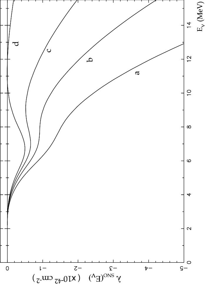
Figure 1: The function $\lambda_{{\scriptscriptstyle SNO}}{{\scriptstyle(E_{\nu})}}\;{\rm vs}$ the neutrino energy for $R^{{\scriptscriptstyle CC}}_{{\scriptscriptstyle SNO}}/R^{{\scriptscriptstyle NC}}_{{\scriptscriptstyle SNO}}=4.50$ (a), 3.41 (b), 2.80 (c), 2.31 (d).

It is possible to estimate the unconstrained rates of SNO using the information that has been published by the collaboration sno_nc . The ES unconstrained rate can be taken to be the same as that constrained by the ${}^{8}\!$B standard shape, since it is determined essentialy from energy independent observations (${\rm cos}\;\theta$ distribution). The NC unconstrained rate $R^{{\scriptscriptstyle NC}}_{{\scriptscriptstyle SNO}}$ can be estimated in terms of the constrained rate $\left(R^{{\scriptscriptstyle NC}}_{{\scriptscriptstyle SNO}}\right)_{{\scriptscriptstyle cons}}$ and the corresponding total fluxes that have been reported by the collaboration:

$$R^{{\scriptscriptstyle NC}}_{{\scriptscriptstyle SNO}}=\frac{\left(\phi^{{\scriptscriptstyle NC}}_{{\scriptscriptstyle SNO}}\right)}{\left(\phi^{{\scriptscriptstyle NC}}_{{\scriptscriptstyle SNO}}\right)_{{\scriptscriptstyle cons}}}\left(R^{{\scriptscriptstyle NC}}_{{\scriptscriptstyle SNO}}\right)_{{\scriptscriptstyle cons}}\;,$$

where $\phi^{SNO}_{NC}=6.42\pm 1.67\times 10^{-6}{\rm cm^{-1}s^{-1}}$ and $(\phi^{SNO}_{NC})_{{\scriptscriptstyle cons}}=5.09\pm 0.63\times 10^{-6}{\rm cm^{-1}s^{-1}}$ are the total unconstrained and constrained NC fluxes, respectively. Finally, the CC unconstrained rate is calculated considering that the total number of signal events is the same as for the constrained analysis. Taking these considerations properly into account, we estimate the ratio of unconstrained rates to be

$$R^{{\scriptscriptstyle CC}}_{{\scriptscriptstyle SNO}}/R^{{\scriptscriptstyle NC}}_{{\scriptscriptstyle SNO}}=2.5\pm 0.8\;.$$

The error is large because the error in the estimate of the NC unconstrained rate in terms of the unconstrained total NC flux is large. Nontheless, the central value is well above the lower limit of 2.31 given above, and indicates that the need for active oscillations is favored.

If the forthcomming results from SNO confirm that $R^{{\scriptscriptstyle CC}}_{{\scriptscriptstyle SNO}}/R^{{\scriptscriptstyle NC}}_{{\scriptscriptstyle SNO}}$ is actually larger than the limit we found using the estimates of bahcall_web for the (response-averaged) cross-section, then the probability transition of solar $\nu_{e}$ into an active neutrino must be different from zero. Consequently, it is not possible to explain the experimental CC and NC results of the collaboration claiming only spectral distortion at the Earth and/or oscillations into sterile neutrinos. It is important to notice that we arrived to this conclusion without assuming that ${\cal P}_{e,a}{{\scriptstyle(E_{\nu})}}$ are constant.

A systematic calculation of the shape of the ${}^{8}\!$B neutrino spectrum has been presented in shape , together with an estimation of the theoretical and experimental uncertainties. No such precise knowledge has been required in our approach, based in the analysis of the negativeness of the integrand in Eq. (24).

IV Model Independent analysis of SK and SNO

In this section, we will use the elastic scattering measurement of SK instead of the corresponding measurement of SNO because it has a smaller error. Equivalently to Eq. (13), we have

$$R^{{\scriptscriptstyle ES}}_{{\scriptscriptstyle SK}}=\overline{\sigma}^{\;{\scriptscriptstyle ES}}_{{\scriptscriptstyle SK}}\;\phi^{{\scriptscriptstyle ES}}_{{\scriptscriptstyle SK}}\;,$$ (25)

with definitions like those given in Eq. (14).

As noted by Fogli et al. fogli , the response functions of SNO and SK behave quite similarly if appropiate thresholds are used. In this way the equality of $\langle{\cal P}_{e,a}\rangle^{ES}_{SK}$ and $\langle{\cal P}_{e,a}\rangle^{CC}_{SNO}$ can be ensured. As discussed in the previous section and noticed in ref. bandy1 , this equality can also be stablished independently of the kinetic energy threshold if the energy independence of the ${\cal P}_{e,a}{{\scriptstyle(E_{\nu})}}$ is adopted. Here we follow this approach. Accordingly, Eqs. (15), (19), and (25) can be rewritten as follows:

$$r_{{\scriptscriptstyle ES}} = x+\rho\;y\;,$$

$$r_{{\scriptscriptstyle CC}} = x\;,$$

$$r_{{\scriptscriptstyle NC}} = x+y\;,$$ (26)

where $r_{{\scriptscriptstyle ES}}$, $r_{{\scriptscriptstyle CC}}$, and $r_{{\scriptscriptstyle NC}}$ are the total rates normalised to the SSM predictions:

$$R_{{\scriptscriptstyle SSM}}^{{\scriptscriptstyle ES}} = \overline{\sigma}^{{\scriptscriptstyle ES}}_{{\scriptscriptstyle SK}}\;\phi_{{\scriptscriptstyle SSM}}\;,$$

$$R_{{\scriptscriptstyle SSM}}^{{\scriptscriptstyle CC,NC}} = \overline{\sigma}^{{\scriptscriptstyle CC,NC}}_{{\scriptscriptstyle SNO}}\;\phi_{{\scriptscriptstyle SSM}}\;.$$ (27)

We have introduced the variables $x\equiv f{\cal P}_{e}$ and $y\equiv f{\cal P}_{a}$, which represent the relevant degrees of freedom of the problem. Since ${\cal P}_{e,a}$ are constants, then $0\leq{\cal P}_{e}+{\cal P}_{a}\leq 1$.

From Eq. (IV), $r_{{\scriptscriptstyle NC}}$ can be expressed in terms of $r_{{\scriptscriptstyle CC}}$ and $r_{{\scriptscriptstyle ES}}$ :

$$r_{{\scriptscriptstyle NC}}=\frac{1}{\rho}\left[r_{{\scriptscriptstyle ES}}-(1-\rho)\;r_{{\scriptscriptstyle CC}}\right]\;,$$ (28)

which is valid for any value of $x$ and $y$ barger .

We define the $\chi^{2}$ function

$$\chi^{2}=\sum_{X}\frac{(r_{X}{\scriptstyle(x,y)}-r^{{\scriptscriptstyle exp}}_{X})^{2}}{\sigma_{X}^{2}}\;,$$ (29)

where $r_{X}{\scriptstyle(x,y)}$ are given in Eq. (IV). Here, $r^{{\scriptscriptstyle exp}}_{X}$ and $\sigma_{X}$ are the experimental values for the normalised rates and their errors respectively sno_nc ; sno_cc ; superk :

$$r^{{\scriptscriptstyle exp}}_{{\scriptscriptstyle SK}} = 0.459\pm 0.017$$

$$r^{{\scriptscriptstyle exp}}_{{\scriptscriptstyle CC}} = 0.349\pm 0.021$$

$$r^{{\scriptscriptstyle exp}}_{{\scriptscriptstyle NC}} = 1.008\pm 0.123\;.$$ (30)

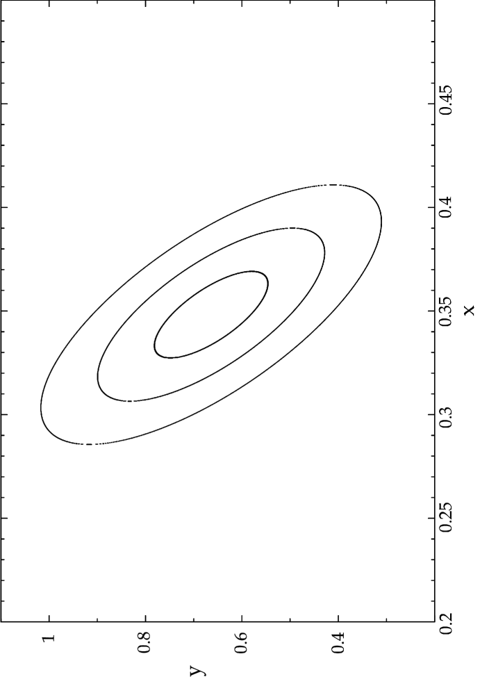
Figure 2: Contours for $\Delta\chi^{2}=1,\;4$, and 9 of allowed values for $x=f\;{\cal P}_{e}$ and $y=f\;{\cal P}_{a}$.

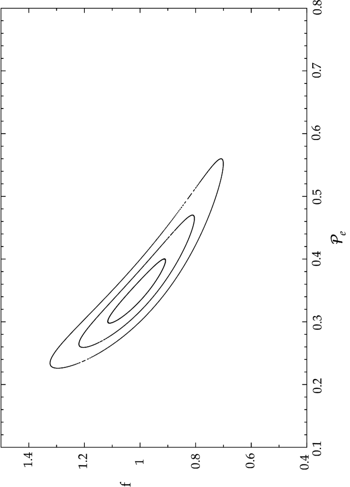
Figure 3: Contours for $\Delta\chi^{2}=1,\;4$, and 9 of allowed values for $f$ and ${\cal P}_{e}$ obtained from mapping the corresponding contours of Fig. 2 with the condition ${\cal P}_{e}+{\cal P}_{a}=1$.

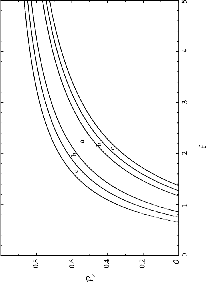
Figure 4: Regions of allowed values of $f$ and ${\cal P}_{s}$ at (a) 68$\%$; (b) 95$\%$, and (c) 99$\%$ C.L.

Letting $x$ and $y$ vary as free parameters, we find the minimum value of $\chi^{2}$ ($\chi^{2}_{min}=0.0039$), and the $\Delta\chi^{2}=1,\;4$, and 9 contours for these parameters as shown in Fig. 2. The projection of these contours on the $x$, and $y$ axes ($N_{DF}=1$ in each case), give their $1\sigma$, $2\sigma$, and $3\sigma$ ranges rpp . The best fit values along with their $1\sigma$ errors are

$$x = 0.35\pm 0.02\;,$$

$$y = 0.66\pm 0.11\;.$$ (31)

The previous values times the SSM total ${}^{8}\!$B flux ($\phi_{{\scriptscriptstyle SSM}}=5.05\times 10^{6}{\rm cm}^{-2}s^{-1}$), give the $\nu_{e}$ and $\nu_{a}$ components of the flux which are consistent with the values reported by SNO sno_nc .

When $f=1$, i.e., there is no discrepancy between the SSM and the true total ${}^{8}\!$B neutrino flux, Ec.(31) gives the 1$\sigma$ ranges for the quantities ${\cal P}_{e}$ and ${\cal P}_{a}$. In this case the sum ${\cal P}_{e}+{\cal P}_{a}$ is consistent with being equal to one.

Let us now assume that there exist oscillations only among active states. Then, we have ${\cal P}_{e}+{\cal P}_{a}=1$, there is also no deformation of the spectrum produced in the Sun ($\zeta{{\scriptstyle(E_{\nu})}}=1$), and $f=x+y$. We obtain the $1\sigma$, $2\sigma$, and $3\sigma$ ranges for $f$ and ${\cal P}_{e}$ from the contours in Fig. 3, built by mapping the contours of Fig. 2 to the plane $f\;{\rm vs}\;{\cal P}_{e}$ using the constriction ${\cal P}_{e}+{\cal P}_{a}=1$. These contours coincide with those found in ref bandy1 directly from Eq. (IV), with $y$ replaced by $f-x$.

From Fig. 3 it can be seen that, by including the NC measurement in the analysis, a significant improovement has been achieved in the $1\sigma$ error bar of $f$ with respect to the one obtained using only the SK and the SNO CC data fogli . The best fit values and their $1\sigma$ ranges are

$$f = 1.01^{+0.11}_{-0.09}$$

$${\cal P}_{e} = 0.34^{+0.05}_{-0.04}$$ (32)

Impossing the less stringent condition $\alpha\leq({\cal P}_{e}+{\cal P}_{a})\leq 1$, with $0\leq\alpha\leq 1$ the value of $f$ will be bounded by

$$x+y\leq f\leq\frac{x+y}{\alpha}\;,$$ (33)

from where we see that allowing for a non vanishing probability to oscillate into a sterile neutrino ($\alpha\neq 1$), we have larger upper bound for $f$. Assuming that ${\cal P}_{e}+{\cal P}_{a}+{\cal P}_{s}=1$, we have that

$${\cal P}_{s}=1-\frac{x+y}{f}\;.$$ (34)

From the dispersion of $x$ and $y$ we can find allowed regions in the ${\cal P}_{s}\;{\rm vs}\;f$ plane, corresponding to the 68, 95, and 99 $\%$ confidence levels. As shown in Fig. 4, these regions are not bounded and hence it is not possible to determine $f$ and ${\cal P}_{s}$ with the existing data barger .

V Conclusions

In this work we have examined the relation between the observed quantities $\phi^{{\scriptscriptstyle CC}}_{{\scriptscriptstyle SNO}}/\phi^{{\scriptscriptstyle NC}}_{{\scriptscriptstyle SNO}}$, $\phi^{{\scriptscriptstyle CC}}_{{\scriptscriptstyle SNO}}/\phi^{{\scriptscriptstyle ES}}_{{\scriptscriptstyle SNO}}$ with the flavor fractional $\nu_{e}$ content of the fluxes measured through the ES and NC reactions. When combined with the hypothesis of a non distorted ${}^{8}\!$B spectrum the measurement gives a clear signal of active flavor transformation. As we also show, when available, the SNO experimental rates unconstrained by the ${}^{8}\!$B standard shape, combined with the cross-section as calculated in ref.bahcall_web , could give conclusive evidence for active oscillations, even for a non constant ${\cal P}_{e}{{\scriptstyle(E_{\nu})}}$.

Finally a model independent analysis including the latest SK and SNO data is performed under the assumption of constant ${\cal P}_{e,a}{{\scriptstyle(E_{\nu})}}$, with and without the condition ${\cal P}_{e}+{\cal P}_{a}=1$. Our result agrees with ref. barger in the sense that no conclusion can be drawn with the present data about the sterile neutrino content of the solar neutrino flux.

References

(1)The SNO Collaboration, R. Ahmad et al.
Phys. Rev. Lett. 7, 649 (2002).
(2)C. E. Ortiz, A. Garcia, R. A. Waltz, M. Bhattacharya,
and A. K. Komives, Phys. Rev. Lett. 85, 2909 (2000).
(3)The SNO Collaboration, R. Ahmad et al.
Phys. Rev. Lett. 87, 071301 (2001).
(4)Super-Kamiokande Collaboration, S. Fukuda
et al., Phys. Rev. Lett. 86, 5651 (2001).
(5)J. N. Bahcall, M. C. Gonzalez-Garcia, and C.
Peña-Garay, J. High Energy Phys. 07, 054 (2002); P. C.
Holanda and A. Yu. Smirnov hep-ph/0205241.
(6)A. Bandyopadhyay, S. Choubey, S. Goswami, and,
D.P. Roy, Phys. Lett. B 540, 14 (2002).
(7)J. N. Bahcall, S. Basu, and M. H. Pissoneault,
Astrophys. J. 55, 990 (2001).
(8)We used the tabulated values for the
cross sections found at the URL http://www.sns.ias.edu/ jnb/SNdata.
(9)G. L. Fogli, E. Lisi, D. Montanino, and, A. Palazzo,
Phys. Rev. D 64, 093007 (2001), ibid., 65,
117301, (2002).
(10)Particle Data Group, D. E. Groom et al.,
Eur. Phys. J. High Energy Phys. 05, 015 (2001);
Probability and Statistics sections.
(11)V. Barger, D. Marfatia, and K. Whinsant,
Phys. Rev. Lett. 88, 011302 (2002).
(12)J. N. Bahcall, E. Lisi, D. E. Alburger,
L. De Braeckleer, S. J. Freedman, and J. Napolitano, Phys. Rev. C
54, 411 (1996).
(13)P. Creminelli, G. Signorelli, A. Sturmia,
, hep-ph/0102234, v3 22 April 2002 (addendum 2).
(14)P. Aliani et al, hep-ph/0205053
(15)A. Sturmia, C. Cattadori, N. Ferrari,
F.Vissani, hep-ph/0205261.
(16)G.L. Fogli, E. Lisi, A. Marrone, D. Montanino,
A. Palazzo, Phys. Rev. D 66, 053010 (2002).
(17)M. Maltoni, T. Schwetz, M.A. Tortola,
J.W.F Valle, hep-ph/0207227.