Abstract

We present a short review of the existing evidence in favor of neutrino mass and neutrino oscillations which come from different kinds of experiments. We focus our attention in particular on solar neutrinos, presenting a review of some recent analysis of all available neutrino oscillation evidence in Solar experiments including the recent $SNO\ CC$ and $NC$ data. We present in detail the power of the reactor experiment KamLAND for discriminating existing solutions to the SNP and giving accurate information on neutrino masses and mixing angles.

Expanded version of the contribution to appear in the Proceedings of ”Third Tropical Workshop on Particle Physics and Cosmology: Neutrinos, Branes and Cosmology (Puerto Rico, August 2002)”

$\star$ email: paul@lcm.mi.infn.it, vito.antonelli@mi.infn.it, marco.picariello@mi.infn.it, torrente@cern.ch

1 Introduction

Neutrino has a long and fascinating history that started more than seventy years ago, when Pauli postulated its existence [1] to explain the data about the high energy part of the $\beta$ decay spectrum. Since then the main issue was to discriminate wether neutrino is a massive or massless particle and eventually to find the value of its mass.

In this work we briefly review the main steps that have been done towards the solution of the neutrino mass puzzle and the different kind of experiments that have been studying it. Then we remind and critically discuss the essential data that have been obtained in this last exciting period and the ones that should be presented very soon, focusing in particular our attention on solar and reactor neutrino physics. We also present the salient aspects of the phenomenological analysis of these data that have been developed by our group, with the aim to understand at which level of accuracy we can determine the values of the mixing parameters and how we can use the results of the forthcoming experiments to improve this accuracy.

The first studies of neutrino mass, performed in the 40th [2], were based on the so called Fermi-Perrin method of observation of the $\beta$ spectrum near the end point and they gave the limit $m_{\nu}\leq 500\,{\rm eV}$. This limit has been significantly lowered in the following decades and by now we know, for instance, that $m(\nu_{e})\leq 2.2{\rm eV}$. About ten years later than the first measurement of neutrino mass, Goldhaber in ’58 measured its helicity [3] and proved that the neutrinos pruduced in $\beta$ decays behave like left-handed particles.

An essential idea for the understanding of neutrino properties was the oscillation hypothesis introduced by Pontecorvo in ’57 [10]. He conjectured that the neutrino states produced in weak interactions could be superpositions of two different states of Majorana neutrinos, having different values of the mass; therefore there could be an oscillation from one neutrino state into another, in a way very similar to what happens in a neutral kaon system. This revolutionary idea (implying the existence of at least one mass eigenvalue different from zero for neutrinos) has been further developed in a series of works [11] and it has been confirmed by many experimental evidences in the following years, as we will see in the rest of this paper. Therefore, by now, we are almost sure that neutrinos are massive and oscillating particles.

The experimental hints in favor of a non zero neutrino mass cannot be accomodated in the usual “minimal” version of the Standard Model of electroweak interactions, in which neutrino is simply a left-handed particle and it is impossible to build a renormalizable neutrino mass term. On the other hand, the existence of such a mass term is predicted in most of the theories beyond the Standard Model, like, for instance, supersymmetric and unified theories. Even if the main issue whether neutrino is massive or not seems to be solved, there are still essential theoretical questions to answer. We don’t know yet, for instance, whether neutrino is a Dirac or Majorana particle, neither we have an unique explanation of the reason for which it is so lighter than all the other known massive particles. The mechanism usually invoked to explain neutrino lightness is the so called see-saw mechanism [4], but there are also other possible alternative explanations. We don’t know yet the absolute value of neutrino masses (experiments up to now can only put upper limits and give information on the mass differences) and which is the exact structure of neutrino mass spectrum. We are not able, for instance, to decide whether we are in presence of “normal” or “inverted hierarchy” or if the masses are “quasi degenerate” [5].

For all these reasons, we can say that in the following years neutrino physics will continue to be an ideal playground for testing different theories beyond the Standard Model, like, for instance, the supersymmetric and unified theories [6] or the ones predicting the existence of large extradimensions [12]. This last class of models, which become very popular in the last years, have important consequences also for neutrino phenomenology. For instance, they predict the existence of an infinite tower of sterile neutrinos and they can give rise to mechanism explaining the lightness of neutrino mass, similarly to the see-saw, but without the need of having a very high mass scale. However the recent experimental results, mainly from cosmology, put very stringent constraints on the large extradimension theories and ruled out the simpler versions of these models. .

The experiments aiming to measure neutrino mass or at least to find evidences that it is different from zero can be classified in three big categories:

• the direct kinematical searches;

• the searches of neutrinoless double $\beta$ decay;

• the experiments looking for neutrino oscillations as a proof that neutrinos are massive.

The direct kinematical searches are performed by looking at the high energy part of the ${}^{3}H\,\beta$-decay spectrum. The present limits on the values of $\nu_{\tau}$ and $\nu_{\mu}$ masses are [8, 9]:

$$m(\nu_{\tau}) < 18.2\quad{\rm MeV}$$

$$m(\nu_{\mu}) < 190\quad{\rm KeV}\,.$$ (1)

The best limits for the mass of the electron neutrino, instead, have been obtained from the Mainz and the Troitsk [23, 24] experiments that have found $m(\nu_{e})<2.2\quad{\rm eV}$. In future many experiments will try to lower this limit. In particular there is a great expectation for KATRIN (the Karlsruhe Tritium Neutrino experiment) [25], that should start the data taking in 2007 and improve the sensitivity down to $0.35\,{\rm eV}$.

The search for neutrinoless double $\beta$ decays is very important because the observation of these decays (violating by two units the lepton number conservation) would imply, under the assumption of CPT invariance, the Majorana nature of neutrino [19, 18]. The most stringent limits available at the moment for the effective Majorana mass come from the Heidelberg-Moskow collaboration [21] $\langle m_{\nu}\rangle<0.35\,{\rm eV}$ and from IGEX (International Germanium Experiment) [22] $\langle m_{\nu}\rangle<0.33-1.35\,{\rm eV}$.

The effective Majorana mass is given by:

$$\left|\langle m\rangle|=|m_{1}|U_{e1}|^{2}+m_{2}|U_{e2}|^{2}e^{i\alpha_{21}}+m_{3}|U_{e3}|^{2}e^{i\alpha_{31}}\right|,$$ (2)

where $m_{i}$ indicate the values of the mass eigenstates, the $U_{ei}$ are elements of the Pontecorvo-Maki-Nakagawa-Sakata mixing matrix and $\alpha_{21},\alpha_{31}$ are the two additional CP violating Majorana phases. The masses and the elements of the mixing matrix entering equation (2) can be expressed in terms of the mass differences and mixing angles that can be recovered from the experiments on solar, atmospheric and reactor neutrinos. Thus, given these experimental inputs, the value of $|\langle m\rangle|$ depends on the ones of $m_{1}$ and of the Majorana phases and on the general structure of neutrino mass spectrum (i.e. normal or inverted hierarchy or quasi degenerate case). In particular one can get interesting lower bounds in the cases of inverted hierarchy and quasi degenerate mass spectrum and a stringent upper bound [45] (smaller than $10^{-2}{\rm eV}$) in the case of normal hierarchy. The NEMO3 [42] experiment and the criogenic detector CUORICINO [20] are expected to reach sensitivity of the order of $10^{-1}{\rm eV}$ and even an order of magnitude better is planned for the next generation experiments [20, 44] CUORE, GENIUS, EXO, MAJORANA and MOON. Therefore, there is the hope that the results of these future experiments, complemented with the information on the absolute value of the masses that could come from KATRIN and from cosmology, could be used to recover hints of CP violation in the leptonic sector or to discriminate between the different possible structures of the mass spectrum. For a more detailed analysis of the present situation and the future perspectives of neutrinoless double $\beta$ decays we refer the interested reader to the work [46] and the references contained in it.

A first group of experiments looking for oscillation signals use neutrino fluxes produced at accelerators and nuclear reactors. They are usually distincted in long- and short baseline, according to the distance existing between the neutrino production point and the detector. Many short baseline accelerator experiments, like NOMAD [26] and CHORUS [27] at Cern, didn’t find any signal of oscillation and, consequently, they gave important constraints on the possible values of the mixing parameters. Between the reactor experiments, it is worthwhile to remember the results of CHOOZ [28] and Palo Verde [30]. At CHOOZ a beam of reactor $\bar{\nu}_{e}$ was sent to a detector located about 1 Km far away and it was detected through the reaction $\bar{\nu}_{e}+p\to e^{+}+n$. No evidence of oscillation was found and these results can be used to exclude a significant part of the mixing parameters plane. In particular they tell us that $\Delta m^{2}$ must be smaller than $10^{-3}eV^{2}$, unless the values of the mixing angle are very small. The CHOOZ data can be used also to fix an upper limit for the quantity $sin^{2}(\theta)$, where $sin^{2}\theta$ coincides with $|U_{e3}|^{2}$ in the case of normal hierarchy and $sin^{2}\theta\equiv|U_{e1}|^{2}$ for neutrinos with inverted hierarchy mass spectrum.

The opposite situation took place in the case of LSND [31], a short baseline accelerator experiment performed with a neutrino beam produced at the Los Alamos meson physics facility (LAMPF). This experiment found evidences for two kind of oscillation signals: that is an excess of $\bar{\nu}_{e}$ in the beam of $\bar{\nu}_{\mu}$ produced by the decay at rest of the $\mu^{+}$ (obtained as secondary products of the proton accelerator beam), and a signal of oscillations into $\nu_{e}$ of the $\nu_{\mu}$ produced by the $\pi^{+}$ decay in flight. The LSND result, if confirmed, would be a clear indication of oscillation with very high values of the mass difference, up to $\Delta m^{2}\simeq 1{\rm eV}^{2}$. To reconciliate this result with the ones coming from solar and atmospheric neutrinos (that we are going to present), one would have to postulate the existence of at least one sterile neutrino in addition to the usual three active ones. However, up to now there have been no independent confirmations of the LSND results. The KARMEN experiment [33], performed at the Rutherford Laboratories, explored a significant part of the mixing parameter space proposed by LSND and it didn’t find any signal of oscillation . A new experiment MiniBoone [35, 36] just started running and it shuold soon produce data. It has been projected in such a way to test definitely the validity of LSND results.

A new generation of very long baseline experiments became available in the last years. The forerunner of them is K2K [37, 38], that uses a neutrino beam produced at the Japan kaon facility KEK and detected at the Kamioka site. Up to now K2K has detected 56 events instead of the expected value in absence of oscillations, that is $80^{+7.3}_{-8}$. This is a confirmation of neutrino oscillations (the null oscillation probability is less than $1\%$). Moreover the best fit point [38] values for the mass difference and the mixing angle ($\Delta m^{2}=2.8\times 10^{-3}{\rm eV}^{2}$ and $\sin^{2}2\theta=1$) are in good agreement with the results of atmospheric neutrino experiments. Two similar projects have been already approved and will become available in the near future: one of them is a neutrino beam from CERN to the Gran Sasso Labs [13] and the other one is in the States [14] (from FNAL to Soudan). The long baseline accelerator experiments will probably give an important confirmation of the oscillation evidences coming up to now from the study of solar and atmospheric neutrinos. They are also expected to find in an unambiguous way indications of oscillation from appearance signals. In the long baseline experiment one has in addition the opportunity of choosing the specific characteristic of the beam; hence they can be used to perform precision measurements. For instance they should be useful to study the value of the mixing angle $\theta_{13}$, relevant for eventual CP violation. The present limit on the measurement of this angle coming from CHOOZ ($\theta_{13}\leq 9$ degrees), could be lowered to the level of about $5$ degrees at ICARUS, one of the two experiments that will use the CERN-Gran Sasso beam.

Important result should very soon come also from the long baseline reactor experiment kamLAND [48], that could in principle give a definite solution to the solar neutrino problem, as we are going to see in the following.

The two main categories of experiments looking for oscillation signals are the ones that study the atmospheric and the solar neutrinos.

The flux and the angular distribution of electronic and muonic neutrinos produced in the atmosphere, in the processes generated by cosmic rays, is known with quite a good accuracy [15], taking into account the number and the properties of cosmic rays and the important geomagnetic effects. This input information are essential, because most of the atmospheric neutrino experiments measure the value of the double ratio $R=\frac{(\mu/e)_{data}}{(\mu/e)_{MC}}$. The numerator and denominator are, respectively, the experimental and the Monte Carlo computed values of the ratio between the events generated by muonic neutrinos (and antineutrinos) and the ones generated by electronic neutrinos (antineutrinos).

At present there are different experiments running on atmospheric neutrinos and most of them are essentially water Cherenkov detectors (like Kamiokande [49, 50, 51, 52], Super-Kamiokande  [53, 54, 55, 56], IMB [57]) or iron plate calorimeters (like Soudan II [17] and in the past years Frejus [59] and Nusex [61]). Clear evidences of oscillation have been found at Kamiokande, Super-Kamiokande (SK), IMB and Soudan II and also at the MACRO [16] experiment at Gran Sasso.

Here we recall the results of SK, which are based on a very high statystic and are, in any case, in good agreement with the other atmospheric experiments which found oscillation signals. The SK results are $R=0.638\pm 0.016\pm 0.050$ for the Sub-GeV events and $R=0.658^{+0.030}_{-0.028}\pm 0.078$ for the Multi-GeV events. Another interesting observable is the up-down asymmetry between the up going events, in which the neutrino crossed the Earth before interacting in the detector, and the down going ones: $A_{e,\mu}=(\frac{U-D}{U+D})$. The experimental value of this quantity is consistent with zero for the electronic neutrinos, while for the muonic ones the day-night asymmetry for high values of the momenta is a decreasing negative value. This result is a clear indication of a reduction of the flux of muonic neutrinos and antineurinos that arrive to the detector after crossing the Earth. The most natural explanation of this phenomenon is the possibility that the muonic neutrinos oscillate into other flavors and the oscillation probability is greatly enhanced by the interaction with matter.

The last group of experiments is that of the experiments observing the neutrinos coming from the Sun. We will discuss them in detail in the rest of the paper.

1.1 History of the solar neutrino problem

The first experiment on solar neutrinos, Homestake [65], started at the end of the $`60s$ using the inverse $\beta$ decay on chlorine ${}^{37}Cl+\nu_{e}\to^{37}Ar+e^{-}$. The threshold energy was $E_{thr}\simeq 0.81{\rm\mbox{\rm MeV}}$, hence it was sensitive to the pep, ${}^{7}Be$, ${}^{8}B$ and hep components of the solar neutrino flux. The results were really surprising, because Homestake found a deficit of the solar neutrino flux of more than $60\%$ that predicted by the Solar Standard Model (SSM). The updated value of the ratio $R$, between the experimental results and the SSM prediction [66], for the chlorine experiment is $R=0.34\pm 0.03$. This result raised fundamental questions: what happens to solar $\nu$ on their way to earth? Eventually, could the SSM be wrong?

The Homestake indication was confirmed by similar experiments, SAGE [70] in Russia and GALLEX [71] and later on GNO [72] at the INFN Gran Sasso Labs, which used gallium instead of chlorine. The energy threshold is lower in the gallium experiments ($E_{thr}\simeq 233\,keV$) making them also sensitive to pp neutrinos, which are the main component of the solar neutrino flux. The updated gallium results are [70, 71, 72]:

$$R = 0.60\pm 0.05\quad(SAGE)$$

$$R = 0.58\pm 0.05\quad(GALLEX-GNO)\,.$$ (3)

This confirmation of Homestake results gave a strong support to the neutrino oscillation hypothesis and caused an increase of the interest for this problem. It could be a signal of new physics.

An essential improvement in the knowledge of solar neutrinos came with the advent of the water Cherenkov experiments, Kamiokande [73] and Super-Kamiokande (SK) [74, 75], that looked at the elastic scattering $\nu_{e}+e^{-}\to\nu_{e}+e^{-}$ and confirmed the existence of the “solar neutrino problem” with a very high statistic. In this experiments it was possible to know the direction of the incoming neutrino (by looking at the outgoing direction of the recoil electron) and also to study the energy and angular spectrum and the day night asymmetries. The energy threshold for these experiments was quite high (5 MeVfor SK) and therefore they were sensitive only to the high energy component of the neutrino flux, that is ${}^{8}B$ and hep neutrinos. Their results confirmed the existence of a deficit in the electron neutrinos reaching the detector. The SK result for the energy spectrum and the small values of the day-night asymmetries were also very important to put strong constraints on the possible values of the mixing parameters.

After the publication of SK data it was clear that there was a deficit of solar electron neutrinos reaching the Earth, with respect to the flux predicted by SSM. The oscillation hypothesis was considered the most plausible explanation of this phenomenon, but there were still different regions allowed by the experiments in the mixing parameter plane, as we will see in detail.

1.2 The post SNO situation

The real breakthrough was due to the SNO experiment that published its first data in 2001 [76] ( see also [82]). SNO is a deuterium Cherenkov detector designed to look simultaneously at three different reactions:

$$\begin{array}[]{lllll}\nu_{e}+d&\to&e^{-}+p+p&\text{{\sl(Charged Current)};}\\ \nu_{x}+d&\to&e^{-}+n+p&\text{{\sl(Neutral Current)};}\\ \nu_{x}+e^{-}&\to&\nu_{x}+e^{-}&\text{{\sl(Elastic Scattering)}.}\end{array}$$ (4)

The first reaction (CC) receives contribution only from the electron neutrino, while the others (NC and ES) are sensitive to all neutrino flavors. This experiment gives the first direct model independent measurement of the total solar neutrino flux reaching the Earth (through the NC observation) and at the same time, comparing this flux with the one of $\nu_{e}$ recovered from CC, it offers a strong evidence of the oscillation of $\nu_{e}$ into other active neutrinos.

During its first phase of working [76] SNO observed the charged current and elastic scattering events, with an energy threshold for electron detection of 6.75 MeV. The $\nu_{e}$ flux measured from CC, after 241 days of running, was: $\Phi_{\nu_{e}}^{CC}=1.75\pm 0.07(stat.)^{+0.12}_{-0.11}(syst.)\times 10^{6}cm^{-2}s^{-1}$. The ratio between this value and the SSM prediction was $R=0.35\pm 0.03$. In the SNO experiment the neutrino flux can be recovered also from the elastic scattering, using the relation :

$$\Phi_{\nu}^{ES}=\Phi_{\nu_{e}}^{ES}+0.154\sum_{i=\mu,\tau}\Phi_{\nu_{i}}^{ES}.$$ (5)

The value of the total neutrino flux recovered from the elastic scattering at SNO and also, with a better statistics, at SK doesn’t agree with the $\nu_{e}$ flux obtained from SNO CC. The comparison of the two results gives:

$$\sum_{i=\mu,\tau}\Phi_{\nu_{i}}^{ES}=3.69\pm 1.13\times 10^{6}cm^{-2}s^{-1}.$$ (6)

This result was the first evidence (at $3\sigma$ level) of the presence of muonic and tauonic neutrinos in a electronic neutrino beam reaching the Earth from the Sun. Therefore it was, up to the present SNO data on NC, the most robust evidence of $\nu_{e}$ oscillation into other active neutrinos. It is also remarkable that the sum of the $\nu_{e}$ and $\nu_{\mu,\tau}$ fluxes give a value in good agreement with the SSM prediction. Consequently the results of SNO phase I also strongly disfavored the hypothesis of pure oscillation into sterile neutrinos.

Observation of neutral current neutrino interactions on deuterium in the SNO experiment has been recently presented  [77, 78]. Using the NC, ES and CC reactions and assuming the ${}^{8}B$ neutrino shape predicted by the SSM, the electron and active non-electron neutrino component of the solar flux at high energies ($\;>$$\sim\;$5 MeV) are obtained. The non-electron component is found to be $\sim 5\sigma$ greater than zero, the standard prediction, thus providing the strongest evidence so far for flavour oscillation in the neutral lepton sector: the agreement of the total flux, provided by the NC measurement with the expectations implies as a by-product the confirmation of the validity of the SSM [67, 69, 68].

The results presented recently by $SNO$ on Solar neutrinos [84] confirm and are consistent with previous evidence from SK and the rest solar neutrino experiments [86, 97, 96, 96, 85]. The CC, ES and NC global and day and night fluxes presented in Refs. [77, 78]. are derived under the assumption that the ${}^{8}B$ spectral shape is not distorted from the SSM prediction. With this assumption the SNO collaboration checks the hypothesis of non-oscillation, or zero $\phi_{\mu+\tau}$ flux.

Different quantities can be defined [80] in order to make the evidence for disappearance and appearance of the neutrino flavours explicit. Letting alone the SNO data, from the three fluxes measured by SNO is possible to define two useful ratios, deviations of these ratios with respect to their standard value are powerful tests for occurrence of new physics. Here we compute the values for $\phi_{CC}/\phi_{ES}$ and $\phi_{CC}/\phi_{NC}$ being specially careful with the treatment of the correlations on the uncertitudes, the inclusion or not of these correlations can affect significantly the results for these ratios (see table II in Ref. [77]. for a complete list of sistematical errors). For the first ratio, from the value from SNO rates  [77, 78]. we obtain

$$\frac{\phi_{CC}}{\phi_{ES}}=0.73^{+0.10}_{-0.07},$$

a value which is $\sim$ 2.7 $\sigma$ away from the no-oscillation expectation value of one. The ratio of CC and NC fluxes gives the fraction of electron neutrinos remaining in the solar neutrino beam, our value is:

$$\frac{\phi_{CC}}{\phi_{NC}}=0.34^{+0.05}_{-0.04},$$

this value is nominally many standard deviations ($\sim 13\sigma$) away from the standard model case [41].

Finally, if in addition to SNO data we consider the flux predicted by the solar standard mode one can define, following Ref.[98], the quantity $\sin^{2}\alpha$, the fraction of ”oscillation neutrinos which oscillated into active ones”, again using the SNO data and fully applying systematic correlations (see table 2 in Ref. [77, 78]), we find the following result:

$$\sin^{2}\alpha=\frac{\phi_{NC}-\phi_{CC}}{\phi_{SSM}-\phi_{CC}}=0.92^{+0.39}_{-0.20}.$$

The SSM flux is taken as the ${}^{8}\rm B$ flux predicted in Ref.[69]. Note that, although consistent with it, this result differs significantly from the number obtained in Ref.[98], this is due to the introduction of systematic correlations in our calculation. The central value is clearly below one (only-active oscillations): the fraction of sterile neutrinos is $\cos^{2}\alpha\raise 1.29167pt\hbox{$\;<$\kern-7.5pt\raise-4.73611pt\hbox{$\sim\;$}}0.28$ (1$\sigma$). Although electron neutrinos are still allowed to oscillate into sterile neutrinos the hypothesis of transitions to only sterile neutrinos is rejected at nearly $5\sigma$, this significance would be reduced if we consider applying a 1-sided analysis to avoid non-physical values.

2 Global analysis of the solar neutrino data

Given all the experimental data that we have just reported, one can say that there is really strong evidence that neutrinos are massive and oscillating particles. Nevertheless, details of the mass pattern still have a long way before being clarified. With this aim in mind, we developed a global analysis of all the available data on solar neutrinos, also including the CHOOZ constraints. Our first purpose was that of determining the regions in the mixing parameter plane that are still compatible with the experiments. In addition to this, we wanted to understand how the forthcoming experiments (in particular Borexino and KamLAND) could improve our knowledge of neutrino mass properties.

We assumed neutrino oscillation as a working hypothesis and considered bidimensional models. For details of our analysis we refer the interested reader to [79, 80]. Here we just report the most salient aspects of our strategy. The analysis is based on the numerical calculation of the expected event rate for every solar neutrino experiment as a function of the mixing parameters and on the comparison between these expected numbers and the experimental data. The statistical analysis is based on the $\chi^{2}$ method its output being contour plots in which one can see which values of the mixing angles and mass differences are still allowed at a given confidence level.

Our calculation can essentially be split into two parts. The first one is the determination of the neutrino transition amplitude, i.e. the probability for an electronic neutrino produced in the Sun to change its flavor before reaching the detector. The other ingredient is the calculation of the detector response functions, that, for a given neutrino energy, depend on the experimental details of the specific detector (i.e. efficiency, resolution, etc.) and on the cross section for the reaction under examination.

The transition amplitude calculation is separated in three parts, corresponding to the neutrino propagation inside the Sun, in the vacuum and in the Earth. For every value of the mixing parameters we compute fully numerically the amplitudes in the Sun and in the Earth, while the one corresponding to the vacuum evolution is computed analytically. The three amplitudes are patched together using the evolution operator formalism [81].

3 The present situation

We included in our analysis [80] the total rates of the chlorine and gallium experiments, together with the different energy bins of SuperKamiokande and with the most recent results of SNO [77, 78]. The results are shown in Fig.1 where we have generated acceptance contours in $\Delta m^{2}$ and $\tan^{2}\theta$. In Table (1) we present the best fit parameters or local minima obtained from the minimisation of the $\chi^{2}$ function. Also shown are the values of $\chi^{2}_{\rm min}$ per degree of freedom ($\chi^{2}/n$) and the goodness of fit (g.o.f.) or significance level of each point (definition of SL as in Ref. [9]). In order to obtain concrete values for the individual oscillation parameters and estimates for their uncertainties, it is preferable to study the marginalized parameter constraints. It is justified to convert $\chi^{2}$ into likelihood using the expression ${\cal L}=e^{-\chi^{2}/2}$, this normalised marginal likelihood is plotted in Figs. (2) for each of the oscillation parameters $\Delta m^{2}$ and $\tan^{2}\theta$. For $\tan^{2}\theta$ we observe that the likelihood function is concentrated in a region $0.2<\tan^{2}\theta<1$ with a clear maximum at $\tan^{2}\theta\sim 0.4$. The situation for $\Delta m^{2}$ is similar. Values for the parameters are extracted by fitting one- or two-sided Gaussian distributions to any of the peaks (fits not showed in the plots). In the case of the angle distribution the goodness of fit of the Gaussian fit is excellent (g.o.f $>99.9\%$) even at far tail distances thus justifying the consistency of the procedure. The goodness of Gaussian fit to the distribution in squared mass, although somewhat smaller, is still good. The values for the parameters appear in Table 1. They are fully consistent and very similar to the values obtained from simple $\chi^{2}$ minimisation.

Method
A) Minimum LMA	$\Delta m^{2}=5.44\times 10^{-5}\ \mbox{\rm eV}^{2}$	$\tan^{2}\theta=0.40$	$\chi_{m}^{2}$ = 30.8	g.o.f.: 80%
B) From Fit	$\Delta m^{2}=4.5^{+2.7}_{-1.4}\times 10^{-5}\mbox{\rm eV}^{2}$	$\tan^{2}\theta=0.40^{+0.10}_{-0.08}$

Table 1: Mixing parameters: A) Best fit in the LMA region and B) from fit to marginal likelihood distributions.

In summary, the direct measurement via the $NC$ reaction on deuterium of ${}^{8}{\rm B}$ neutrinos combined with the $CC$ results have largely confirmed the neutrino oscillation hypothesis. We have obtained the allowed area in parameter space and individual values for $\Delta m^{2}$ and $\tan^{2}\theta$ with error estimation from the analysis of marginal likelihoods.

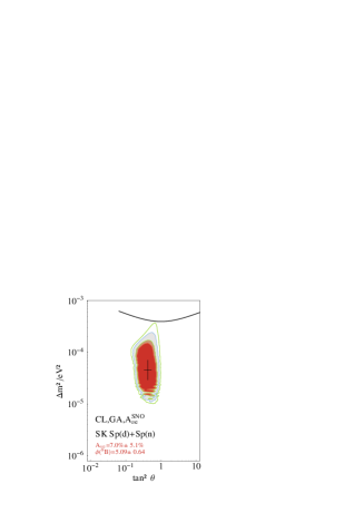
Figure 1: Allowed areas in the two neutrino parameter space. The point with error bars corresponds to best the results from fit to marginal likelihoods. The coloured areas are the allowed regions at 90, 95, 99 and 99.7% CL relative to the absolute minimum. The region above the upper thick line is excluded by the reactor experiments [29].

Figure 2: Marginalized likelihood distributions for each of the oscillation parameters $\Delta m^{2}$ (right), $\tan^{2}\theta$ (left). The curves are in arbitrary units with normalization to the maximum height. Values for the peak position are obtained by fitting two-sided gaussian distrbutions (not showed in the plot). Dashed lines delimit $\pm 1\sigma$ error regions around the maximum.

4 Future scenarios: Borexino

Given this situation, we studied which new information should come in future from the Borexino data [79, 87, 83]. Borexino [88, 89] is a solar neutrino experiment, mainly sensitive to the ${}^{7}Be$ component of the neutrino flux, that should start running in very next years at the Gran Sasso Labs. In Figure 3 the usual contour plots obtained from all the experiments available up to now are superimposed to the contour lines corresponding to different hypothetical possible values of the total rate at Borexino. Note that, for what concerns the data coming from the other solar neutrino experiments, this figure refers to the situation how it was in 2001, before the publication of the last results from SK and from SNO neutral current. As one can see from the picture, Borexino should be able to clarify the situation in the case in which the solution very well is in the small mixing angle region. The situation would be, instead, more complicate in case of LMA or LOW solutions. In these two regions, in fact, the ratio between the Borexino signal and the SSM prediction in absence of oscillations should be between 0.6 and 0.7 . The discrimination power of Borexino increases a lot if we look also at the day-night asymmetry, as one can see from Figure 4. The LOW region is characterized by high values of the asymmetry, that can reach up to $20\%$, while in the LMA region the day-night asymmetry is much lower. Hence, by looking simultaneously at the total rate and at the day-night asymmetry, Borexino should be able to discriminate between the two solutions of the solar neutrino problem that are compatible with the experiments up to now, that is the LMA and the LOW solutions.

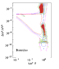
Figure 3: Possible values of the total signal at Borexino. The full lines correspond to a total rate equal respectively to 0.5, 0.6 and 0.7 with respect to the SSM prediction in absence of oscillation. These isosignal lines are superimposed to the contour plots (colored regions) corresponding to the regions allowed at different confidence levels from the other experiments.

5 Future Experiments: Kamland

Another very important experiment, already running, that should significantly improve our knowledge of the mixing parameters relevant for solar neutrinos is KamLAND [48]. In this experiment a flux of low energy $\bar{\nu}_{e}$ produced by different nuclear reactors is sent to a scintillator detector capable of detecting their interactions with protons. Although it not a solar neutrino experiment, KamLAND is sensitive to neutrino oscillations with mixing parameters in the LMA region, that seems to be the solution of the solar neutrino problem preferred by the present data. Therefore, we can hope that KamLAND will soon be able to determine the exact values of the mixing parameters with satisfactory accuracy. The main limitation of KamLAND is its reduced sensitivity to the extreme upper part of the LMA region, that could create problems in the determination of $\Delta m_{12}^{2}$, as discussed in [90, 91] and later on in [92]. For a detailed discussion about KamLAND potentiality and discrimination power we refer the interested reader to [93, 83].

In order to study the potentiality of KamLAND for resolving the neutrino oscillation parameter space, we have developed two kind of analysis. In the first case (Analysis A below) we deal with the KamLAND expected global signal. We asumme that the experiment measure a certain global signal with given statistical and systematic error after some period of data taking (1 or 3 yrs) and perform a complete $\chi^{2}$ statistical analysis including in addition the up-date solar evidence. In the second case, Analysis B, we include the full KamLAND spectrum information. Instead of giving arbitrary values to the different bins, we assume a number of oscillation models characterized by their mixing parameters $(\Delta m^{2},\theta)$. After including the solar evidence we perform the same $\chi^{2}$ analysis as before.

In Fig.4 we graphically show the results of this analysis. They represent exclusion plots including KamLAND global rates, given a hypothetical experimental global signal ratio: respectively strong and medium suppression $S/S_{0}=0.3,0.6$ and no oscillation evidence $S/S_{0}=1.0$ for one and three years of KamLAND data taking. As can be seen in the figures, as the KamLAND experimental signal decreases, the LMA region is singled out. The periodic shape in $\Delta m^{2}$ of the 90 % C.L. (red regions) which becomes apparent in the three-year plot is due to the periodicity of the response function: in order to distinguish among these different equally-likely solutions, one must analyze the energy spectrum, Obviously, only if KamLAND sees some oscillation signal (i.e. $S_{i}/S_{0}<<1.0$ ) does the LMA region become the only solution. If we consider a hypothetical signal closer to 1.0 than 0.3, we see that the LOW region survives, although it is less favored.

In Figs.(5) we graphically show the results of this analysis for a selection of points and for three years of data taking restricting ourselves to the LMA region of the parameter space where, as we have noted before, the KamLAND spectrum information is specially significative. In each plot allowed regions corresponding to different starting points are superimposed, every region is distinguished with a label. The position of initial points is labeled with solid stars.

The first case, study of the KL spectrum alone ($\chi^{2}_{spec,KL}$) is represented by the Fig.(5 left). The allowed parameter space corresponding to each particular point is formed by a number of, highly degenerated, disconnected regions symmetric with respect the line $\tan\theta=1$. These regions can extend very far from the initial point specially in terms of $\Delta m^{2}$ but also in some occasions in terms of $\tan^{2}\theta$. For example the point “A” located at $(\Delta m^{2}=5.7\times 10^{-4},\tan^{2}\theta=0.38)$ gives rise to two sets of thin regions situated respectively at $\Delta m^{2}\sim 10^{-3},10^{-4}$ and a third region situated at $\Delta m^{2}\sim 10^{-5}$ which practically covers the full range $\tan^{2}\theta\sim 0.1-10$. A similar behavior is observed for point “B”. Of course this situation is not very favorable for the future phenomenologist trying to extract conclusions from the KamLAND data. A much comfortable situation is found for points nearer the center of the LMA region. Note how the regions corresponding to the points “D,E” and specially “F” only extend very gently around the initial location.

The results of the full analysis are summarized in Fig.(5, right). The position of the minima of $\chi^{2}$, marked in the plot with crosses, is practically identical to the position of the initial points except in some case where the difference is not significant anyway. The general effect of the inclusion of the solar evidence in the $\chi^{2}$ is the breaking of the symmetry in $\tan^{2}\theta$ as expected and the general reduction of the number of disconnected regions corresponding to each point. Note however that the point “A” still gives rise to a small allowed region situated nearly one order of magnitude smaller in $\Delta m^{2}$. The “B” region is shrinked near its initial location as happens to the rest of points. The conclusion to be drawed from these plots is that KamLAND together with the rest of solar experiments will be able to resolve the neutrino mixing parameters with a precision of $\delta\log\Delta m^{2}\sim\pm 0.1$ practically everywhere. However, for values of $\Delta m^{2}>10^{-4}$ the problem of the coexistence of multiple regions with similar statistical significance will still be present.

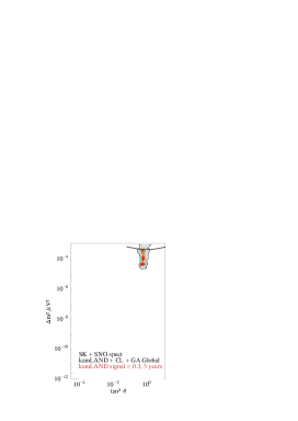
Figure 4: Exclusion plots including KamLAND global rates (Analysis A), given a hypothetical experimental global signal ratio: respectively $S/S_{0}=0.3$. Statistical and assumed systematics ($\sim 5\%$) errors are included. Three year of KamLAND data taking. The colored areas are allowed at 90, 95, 99 and 99.7% CL relative to the absolute minimum. The region above the upper thick line is excluded by the reactor experiments [29].

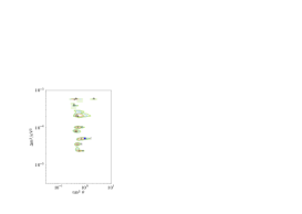
Figure 5: Allowed areas in the two neutrino parameter space after 3 years of data taking in KamLAND (Analysis B). Allowed regions belonging to the same point are labeled with the corresponding letter, the position of the point itself is labeled with a solid star. The colored lines separate allowed regions at 90, 95, 99 and 99.7% CL relative to the absolute minimum. (Left) Results with the KamLAND spectrum alone. (Right) KamLAND spectrum plus solar (CL,GA,SK,SNO) evidence. Crosses are situated in the position of the $\chi^{2}$ minima.

5.1 KamLAND and solar antineutrinos

We have also investigated [94] the possibility of detecting solar antineutrinos with the KamLAND experiment. These antineutrinos are predicted by spin-flavor solutions to the solar neutrino problem. As we saw before, the recent evidence from SNO shows that a) the neutrino oscillates, only around 34% of the initial solar neutrinos arrive at the Earth as electron neutrinos and b) the conversion is mainly into active neutrinos, however a non e,$\mu-\tau$ component is allowed: the fraction of oscillation into non-$\mu-\tau$ neutrinos is found to be $\cos^{2}\alpha=0.08^{+0.20}_{-0.40}$. This residual flux could include sterile neutrinos and/or the antineutrinos of the active flavors.

The KamLAND experiment is potentially sensitive to antineutrinos coming from solar ⁸B neutrinos. Reactor and solar antineutrino signals are shown in Fig.(6). In case of negative results, we find that the results of the KamLAND experiment could put strict limits on the flux of solar antineutrinos $\Phi({}^{8}B)<1.0\times 10^{4}\ cm^{-2}\ s^{-1}$, and their appearance probability ($P<0.2-0.15\%$), respectively after 1-3 years of operation. Assuming a concrete model for antineutrino production by spin-flavor precession in the convective solar magnetic field, this upper bound on the appearance probability implies an upper limit on the product of the intrinsic neutrino magnetic moment and the value of the field $\sim\mu B<10^{-21}$ MeV. For $B\sim 10-100$ kG, we would have $\mu<10^{-11}-10^{-12}\ \mu_{B}$.

In the opposite case, if spin-flavor precession is indeed at work even at a minor rate, the additional flux of antineutrinos could strongly distort the signal spectrum seen at KamLAND at energies above 4 MeV and their contribution should be taken into account. This is graphically shown in Fig.(6)

Ethr	$S_{Sun}$	$S_{Rct}$	Bckg.	P (CL 95)%	P (CL 99)%
6 MeV	616	43	70	0.22	0.23
7 MeV	500	11	65	0.19	0.20
8 MeV	366	2	60	0.21	0.23

Table 2: Expected signals from solar antineutrinos after 3 years of data taking. Reactor antineutrino (no oscillation is assumed) and other background (correlated background) over the same period. The random coincidence background is supposed negligble above these energy thresholds. Upper limits on the antineutrino oscillation probability.

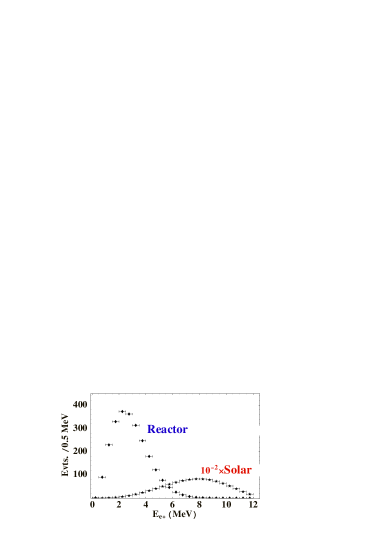
Figure 6: The KamLAND expected positron spectra in absence of oscillations coming from reactor antineutrinos (normalized to three years of data taking). The “solar” positron spectrum is obtained assuming the shape of the ${}^{8}B$ neutrino flux and a total normalization $10^{-2}\times\Phi({}^{8}B)$ (that is, an overall $\nu_{e}-\overline{\nu}_{e}$ conversion probability $\overline{P}\sim 1\%$).

Acknowledgements

One of us, V. A., would like to thank all the organizers of the ”Third Tropical Workshop on Particle Physics and Cosmology: Neutrinos, Branes and Cosmology (Puerto Rico, August 2002)” and in particular J. Nieves, for the kind invitation and for providing a pleasant and stimulating atmosphere. We are glad to thank all the other participants of the conference and mainly E. Lisi, M. Smy and J. Formaggio for very useful discussions.It’s a pleasure to thank also S.T. Petcov for enlightening conversations while this paper was prepared.

References

- [1] See: W. Pauli, in Neutrino Physics (1991), pag. 1, edited by K. Winter, Cambridge University press
- [2] O. Kofoed-Hansen, Phys. Rev. 71, 451 (1947); G. C. Hanna and B. Pontecorvo, Phys. Rev. 75, 451 (1949)
- [3] M. Goldhaber, L. Grodzins and A.W. Sunyar, Phys. Rev. 109, 1015 (1958)
- [4] T. Yanagida, Proc. of the Workshop on Unified Theory and the Baryon Number of the Universe, KEK, Japan, 1979; M. Gell-Mann, P. Ramond and R. Slansky, in Supergravity, p. 315, edited by F. van Nieuwenhuizen and D. Freedman, North Holland, Amsterdam, 1979; R.N. Mohapatra and G. Senjanovic, Phys. Rev. Lett. 44, 912 (1980).
-
[5]
For recent analysis of the possible structure of neutrino mass matrix see,
for instance, the following papers (and the references contained therein):
M. Frigerio, A.Y. Smirnov, arXiv:hep-ph/0202247; M. Frigerio, A.Y. Smirnov, arXiv:hep-ph/0207366; V. Antonelli, F. Caravaglios, R. Ferrari, M. Picariello, arXiv:hep-ph/0207366 (will appear on Phys. Lett. B); G. Altarelli, F. Feruglio, I. Masina, arXiv:hep-ph/0210342; G. Altarelli, F. Feruglio, arXiv:hep-ph/0206077.
For the possibility of future experiments to discriminate between different possible structure of the spectrum see the work [46] - [6] See for instance: T. Fukuyama, N. Okada, arXiv:hep-ph/0205066 ; R. Kitano, arXiv:hep-ph/0204164; B. Bajc, G. Senjanovic and F. Vissani, arXiv:hep-ph/0110310
- [7] S.M. Bilenky and S.T. Petcov, Rev. of Mod. Phys. 59, 671 (1987).
-
[8]
R. Barate et al., Eur. Phys. J. C2, 395 (1998); see also:
J. M. Roney, Nucl. Phys. Proc. Suppl. 91, 287 (2001) - [9] D. E. Groom et al., Eur. Phys. J. C15, 1 (2000)
- [10] B. Pontecorvo, J. Exptl. Theoret. Phys., 33, 549 (1957) [Sov. Phys. JETP 6, 429 (1958)]; B. Pontecorvo, J. Exptl. Theoret. Phys., 34, 247 (1958) [Sov. Phys. JETP 7, 172 (1958)]
- [11] See, for instance: Z. Maki, M. Nakagawa and S. Sakata, Prog. Theor. Phys. 28, 870 (1962); V. Gribov and B. Pontecorvo, Phys. Lett. B 28, 493 (1969); S.M. Bilenky and B. Pontecorvo, Phys. Lett. B 61, 248 (1976); H. Fritzsch and P. Minkowski, Phys. Lett. B 62, 72 (1976); S.M. Bilenky and B. Pontecorvo, Lett. Nuovo Cim. 17, 569 (1976); S.M. Bilenky, J. Hosek and S. T. Petcov, Phys. Lett. B 94, 495 (1980)
- [12] See for instance: N. Arkani-Hamed, S. Dimopoulos, G. R. Dvali and J. March-Russell, Phys. Rev. D 65, 024032 (2002); R. N. Mohapatra, S. Nandi and A. Perez-Lorenzana, Phys. Lett. B 466, 115 (99); R.Barbieri, P. Creminelli and A. Strumia, Nucl. Phys. B 585, 28 (2000); A. Lukas, P. Ramond, A. Romanino and G. G. Ross, Phys. Lett. B 495, 136 (2000); H. Davoudiasl, P. Langacker and M. Perelstein, Phys. Rev. D 65, 105015 (2002); K. R. Dienes, E. Dudas and T. Gherghetta, Nucl. Phys. B 557, 25 (99)
- [13] S. Katsanevas, The CNGS program status and Physics potential, talk given at Neutrino 2002, XXth International Conference on Neutrino Physics and AstroPhysics, May 2002, Munich
- [14] K. Lang [MINOS Collaboration], Nucl. Instrum. Meth. A 461, 290 (2001).
- [15] G. Battistoni, A. Ferrari, T. Montaruli and P. R. Sala, arXiv:hep-ph/0207035;
- [16] M. Giorgini [MACRO Collaboration], arXiv:hep-ex/0210008; G. Giacomelli [MACRO Collaboration], arXiv:hep-ex/0210006; M. Ambrosio et al. [MACRO Collaboration], Phys. Lett. B 434, 451 (1998)
- [17] D. A. Petyt [SOUDAN-2 Collaboration], Nucl. Phys. Proc. Suppl. 110 (2002) 349; W. W. Allison et al. [Soudan-2 Collaboration], Phys. Lett. B 449 (1999) 137
- [18] F. Feruglio, A. Strumia and F. Vissani, Nucl. Phys. B 637 (2002) 345; S. M. Bilenky, S. Pascoli and S. T. Petcov, Phys. Rev. D 64 (2001) 053010; F. Vissani, JHEP 9906 (1999) 022
- [19] S. M. Bilenky and S. T. Petcov, Rev. Mod. Phys. 59, 671 (1987) [Erratum-ibid. 61, 169 (1989)].
- [20] S. Pirro et al., Nucl. Instrum. Meth. A 444 (2000) 71; E. Fiorini, Phys. Rep. 307, 309 (1998).
- [21] H. V. Klapdor-Kleingrothaus et al., Eur. Phys. J. A 12, 147 (2001).
- [22] C. E. Aalseth et al. [16EX Collaboration], Phys. Rev. D 65, 092007 (2002)
- [23] J. Bonn et al., Nucl. Phys. Proc. Suppl. 91, 273 (2001); Ch. Weinheimer et al., Phys. Lett. B460, 219 (1999)
- [24] V. M. Lobashev et al., Nucl. Phys. Proc. Suppl. 91, 280 (2001); V. M. Lobashev et al., Phys. Lett. B460 (1999)
- [25] A. Osipowicz et al, KATRIN letter of intent, arXiv:hep-ex/0109033
- [26] J. Altegoer et al., NOMAD Coll., Phys. Lett. B 431, 219 (1998)
- [27] CHORUS Coll., arXiv hep-ex/9807024
- [28] M. Apollonio et al., CHOOZ Coll., Phys. Lett. B 466, 415 (1999)
- [29] M. Apollonio et al. (CHOOZ coll.), hep-ex/9907037, Phys. Lett. B 466 (1999) 415. M. Apollonio et al., Phys. Lett. B 420 (1998) 397. F. Boehm et al.,Phys. Rev. D62 (2000) 072002 [hep-ex/0003022].
- [30] F. Boehm et al., Phys. Rev. D 64, 112001 (2001)
- [31] M. Sung, Int. J. Mod. Phys. A 16S1B, 752 (2001).
- [32] C. Athanassopoulos et al., LSND Coll., Phys. Rev. Lett. 81, 1774 (1998)
- [33] J. Wolf [KARMEN Collaboration],
- [34] G. Drexlin, talk given at Neutrino 2002, XXth International Conference on Neutrino Physics and Astrophysics, May 2002, Munich
- [35] E. A. Hawker, Int. J. Mod. Phys. A 16S1B, 755 (2001).
- [36] R. Stefanski [MINIBOONE Collaboration], Nucl. Phys. Proc. Suppl. 110, 420 (2002).
- [37] C. Yanagisawa, Nucl. Phys. Proc. Suppl. 95, 130 (2001).
- [38] K. Nishikawa, for the K2K collaboration, talk given at Neutrino 2002, XXth International Conference on Neutrino Physics and Astrophysics, May 2002, Munich
- [39] S. Katsanevas, The CNGS program status and Physics potential, talk given at Neutrino 2002, XXth International Conference on Neutrino Physics and Astrophysics, May 2002, Munich
- [40] J. Rico [ICARUS Collaboration], arXiv:hep-ex/0205028.
- [41] Y. Fukuda et al. [Super-Kamiokande Collaboration], Phys. Rev. Lett. 82, 1810 (1999) J. N. Bahcall, P. I. Krastev and E. Lisi, Phys. Rev. C 55, 494 (1997) J. N. Bahcall and E. Lisi, Phys. Rev. D 54, 5417 (1996) J. N. Bahcall, E. Lisi, D. E. Alburger, L. De Braeckeleer, S. J. Freedman and J. Napolitano, Phys. Rev. C 54, 411 (1996)
- [42] C. Marquet et al. (NEMO3 Coll.), Nucl. Phys. B Proc. Suppl. 87, 298 (2000)
- [43] E. Fiorini, Phys. Rep. 307, 309 (1998)
- [44] H.V. Klapdor-Kleingrothaus et al., J. Phys. G 24, 483 (1998); M. Danilov et al, Phys. Lett. B 480, 12 (2000); L. De Braeckeleer (for the Majorana Coll.), Proceedings of the Carolina Conference on Neutrino Physics, Columbia SC USA, March 2000; H. Ejiri et al, Phys. Rev. Lett. 85, 2917 (2000).
- [45] S. Pascoli, S.T. Petcov, arXiv:hep-ph/0205022 (to be published in Phys. Lett. B)
- [46] S. Pascoli, S.T. Petcov and W. Rodejohann, arXiv:hep-ph/0209059
- [47] V. D. Barger, A. M. Gago, D. Marfatia, W. J. Teves, B. P. Wood and R. Zukanovich Funchal, Phys. Rev. D 65, 053016 (2002)
- [48] A. Piepke [kamLAND collaboration], Nucl. Phys. Proc. Suppl. 91, 99 (2001); P. Alivisatos et al, STANFORD-HEP-98-03 J. Shirai, Start of Kamland, talk given at Neutrino 2002, XXth International Conference on Neutrino Physics and Astrophysics, May 2002, Munich
- [49] S. Hatakeyama et al. [Kamiokande Collaboration], Phys. Rev. Lett. 81, 2016 (1998)
- [50] Y. Oyama, Phys. Rev. D 57, 6594 (1998).
- [51] Y. Fukuda et al. [Kamiokande Collaboration], Phys. Lett. B 335, 237 (1994).
- [52] K. S. Hirata et al. [Kamiokande-II Collaboration], Phys. Lett. B 280, 146 (1992).
- [53] Y. Fukuda et al. [Super-Kamiokande Collaboration], Phys. Rev. Lett. 81, 1562 (1998) [arXiv:hep-ex/9807003].
- [54] T. Kajita [Super-Kamiokande Collaboration], Nucl. Phys. Proc. Suppl. 100, 107 (2001).
- [55] T. Toshito [SuperKamiokande Collaboration], arXiv:hep-ex/0105023.
- [56] S. Fukuda et al. [Super-Kamiokande Collaboration], Phys. Rev. Lett. 85, 3999 (2000) [arXiv:hep-ex/0009001].
- [57] R. Becker-Szendy et al., Nucl. Phys. Proc. Suppl. 38, 331 (1995).
- [58] M. Sanchez [Soudan-2 Collaboration], Int. J. Mod. Phys. A 16S1B, 727 (2001).
- [59] K. Daum [Frejus Collaboration.], Z. Phys. C 66, 417 (1995).
- [60] C. Berger et al. [Frejus Collaboration], Phys. Lett. B 227, 489 (1989).
- [61] M. Aglietta et al. [The NUSEX Collaboration], Europhys. Lett. 8, 611 (1989).
- [62] S. Ragazzi et al., Prepared for 9th Moriond Workshop: Tests of Fundamental Laws (Particle Physics, Astrophysics, Atomic Physics), Les Arcs, France, 21-28 Jan 1989.
- [63] M. Ambrosio et al. [MACRO Collaboration], Phys. Lett. B 517, 59 (2001) [arXiv:hep-ex/0106049].
- [64] G. Giacomelli and M. Giorgini [MACRO Collaboration], arXiv:hep-ex/0110021.
- [65] B. T. Cleveland et al, Astrophys. J. 496, 505 (1998)
- [66] J. N. Bahcall, M. H. Pinsonneault and S. Basu, Astrophys. J. 555, 990 (2001)
- [67] S. Turck-Chieze, Nucl. Phys. Proc. Suppl. 91 (2001) 73. E. G. Adelberger et al., Rev. Mod. Phys. 70 (1998) 1265 [arXiv:astro-ph/9805121]. A. S. Brun, S. Turck-Chieze and P. Morel, arXiv:astro-ph/9806272.
- [68] J.N. Bahcall and M.H. Pinsonneault, Rev. Mod. Phys. 67 (1995) 781.
- [69] J. N. Bahcall, M. H. Pinsonneault and S. Basu, Astrophys. J. 555, 990 (2001) [arXiv:astro-ph/0010346].
- [70] SAGE collaboration, J. N. Abdurashitov et al, Phys. Rev. C 60 055801 (1999) ; SAGE collaboration, V. Gavrin, Solar neutrino results from SAGE, in Neutrino 2000, Proc. of the XIXth International Conference on Neutrino Physics and Astrophysics, Nucl. Phys. B91 Proc. Suppl., 36 (2001)
- [71] GALLEX collaboration, W. Hampel et al, Phys. Lett. B 447, 127 (1999)
- [72] GNO collaboration, M. Altmann et al, Phys. Lett. B 490, 16 (2000); GNO collaboration, E. Bellotti et al, First Results from GNO, in Neutrino 2000, Proc. of the XIXth International Conference on Neutrino Physics and Astrophysics, Nucl. Phys. B91 Proc. Suppl., 44 (2001)
- [73] Kamiokande collaboration, Y. Fukuda et al, Phys. Rev. Lett. 77, 1683 (1996)
- [74] Super-Kamiokande collaboration, S. Fukuda et al, Phys. Rev. Lett. 86, 5651 (2001); M. B. Smy, arXiv:hep-ex/0202020
- [75] M. B. Smy arXiv:hep-ex/0206016.
- [76] SNO collaboration, Q. R. Ahmad et al, Phys. Rev. Lett. 87, 071301 (2001)
- [77] Q. R. Ahmad et al. [SNO Collaboration], arXiv:nucl-ex/0204008.
- [78] Q. R. Ahmad et al. [SNO Collaboration], arXiv:nucl-ex/0204009.
- [79] P. Aliani, V. Antonelli, M. Picariello and E. Torrente-Lujan, Nucl. Phys. B 634, 393 (2002) [arXiv:hep-ph/0111418].
- [80] P. Aliani, V. Antonelli, R. Ferrari, M. Picariello and E. Torrente-Lujan, arXiv:hep-ph/0205053 (will appear on Phys. Rev. D).
- [81] E. Torrente-Lujan, Phys. Rev. D 59 (1999) 093006 [arXiv:hep-ph/9807371]. E. Torrente-Lujan, Phys. Rev. D 59 (1999) 073001; E. Torrente-Lujan, Phys. Lett. B 441, 305 (1998); V. B. Semikoz and E. Torrente-Lujan, Nucl. Phys. B 556, 353 (1999); E. Torrente-Lujan, arXiv:hep-ph/0210037. S. Khalil and E. Torrente-Lujan, J. Egyptian Math. Soc. 9, 91 (2001) [arXiv:hep-ph/0012203]. E. Torrente Lujan, Phys. Rev. D 53, 4030 (1996).
- [82] J. N. Bahcall, M. C. Gonzalez-Garcia and C. Pena-Garay, JHEP 0108, 014 (2001) [arXiv:hep-ph/0106258]; J. N. Bahcall, M. C. Gonzalez-Garcia and C. Pena-Garay, JHEP 0204, 007 (2002) [arXiv:hep-ph/0111150]; A. Y. Smirnov, “Global analysis with SNO: Toward the solution of the solar neutrino problem,”,published in Venice 2001, Neutrino oscillations, 43-64; G. L. Fogli, E. Lisi, D. Montanino and A. Palazzo, Phys. Rev. D 64, 093007 (2001) [arXiv:hep-ph/0106247]; M. Maris and S. T. Petcov, Phys. Lett. B 534, 17 (2002) [arXiv:hep-ph/0201087]; M. Maltoni, T. Schwetz and J. W. Valle, Phys. Rev. D 65, 093004 (2002) [arXiv:hep-ph/0112103]; A. Bandyopadhyay, S. Choubey, S. Goswami and K. Kar, Phys. Lett. B 519, 83 (2001) [arXiv:hep-ph/0106264]; A. M. Gago, M. M. Guzzo, P. C. de Holanda, H. Nunokawa, O. L. Peres, V. Pleitez and R. Zukanovich Funchal, Phys. Rev. D 65, 073012 (2002) [arXiv:hep-ph/0112060]; M. V. Garzelli and C. Giunti, Phys. Rev. D 65, 093005 (2002) [arXiv:hep-ph/0111254].
- [83] P. Aliani, V. Antonelli, R. Ferrari, M. Picariello and E. Torrente-Lujan, arXiv:hep-ph/0205061. P. Aliani, V. Antonelli, R. Ferrari, M. Picariello and E. Torrente-Lujan, arXiv:hep-ph/0206308.
- [84] Q. R. Ahmad et al. [SNO Collaboration], Phys. Rev. Lett. 87 (2001) 071301 [arXiv:nucl-ex/0106015].
- [85] J.N. Abdurashitov et al. (SAGE Coll.) Phys. Rev. Lett. 83(23) (1999)4686.
- [86] R. Davis, Prog. Part. Nucl. Phys. 32 (1994) 13. B.T. Cleveland et al., (HOMESTAKE Coll.) Nucl. Phys. (Proc. Suppl.)B 38 (1995) 47. B.T. Cleveland et al., (HOMESTAKE Coll.) Astrophys. J. 496 (1998) 505-526.
- [87] P. Aliani, V. Antonelli, M. Picariello and E. Torrente-Lujan, Nucl. Phys. Proc. Suppl. 110, 361 (2002) [arXiv:hep-ph/0112101].
- [88] G. Bellini, Recent Developments in the Borexino Project, talk given at Neutrino 2002, XXth International Conference on Neutrino Physics and Astrophysics, May 2002, Munich
- [89] E. Meroni, Nucl. Phys. Proc. Suppl. 100, 42 (2001); G. Ranucci et al. [BOREXINO Collaboration], Nucl. Phys. Proc. Suppl. 91, 58 (2001); S. Bonetti et al [Borexino Coll.], Nucl. Phys. Proc. Suppl. 28 A, 486 (1992)
- [90] A. Strumia and F. Vissani, JHEP 0111 (2001) 048 [arXiv:hep-ph/0109172].
- [91] S. T. Petcov and M. Piai, Phys. Lett. B 533, 94 (2002) [arXiv:hep-ph/0112074].
- [92] S. Schonert, T. Lasserre and L. Oberauer, arXiv:hep-ex/0203013
- [93] P. Aliani, V. Antonelli, M. Picariello and E. Torrente-Lujan, arXiv:hep-ph/0207348.
- [94] P. Aliani, V. Antonelli, M. Picariello and E. Torrente-Lujan, arXiv:hep-ph/0208089. See also: E. Torrente-Lujan, Nucl. Phys. Proc. Suppl. 87, 504 (2000). E. Torrente-Lujan, Phys. Lett. B 494, 255 (2000).
- [95] J. N. Bahcall, M. C. Gonzalez-Garcia and C. Pena-Garay, arXiv:hep-ph/0204314.
- [96] Y. Fukuda et al. [Super-Kamiokande Collaboration], Phys. Rev. Lett. 81, 1158 (1998) [Erratum-ibid. 81, 4279 (1998)] [arXiv:hep-ex/9805021].
- [97] Y. Fukuda et al. [Super-Kamiokande Collaboration], Phys. Rev. Lett. 82, 1810 (1999) [arXiv:hep-ex/9812009].
- [98] V. Barger, D. Marfatia and K. Whisnant, arXiv:hep-ph/0106207. V. Barger, D. Marfatia, K. Whisnant and B. P. Wood, arXiv:hep-ph/0204253. A. Bandyopadhyay, S. Choubey, S. Goswami and D. P. Roy, arXiv:hep-ph/0204286; R. Foot and R. R. Volkas, arXiv:hep-ph/0204265; S. Pascoli and S. T. Petcov, arXiv:hep-ph/0205022. P. C. de Holanda and A. Y. Smirnov, arXiv:hep-ph/0205241; A. Strumia, C. Cattadori, N. Ferrari and F. Vissani, Phys. Lett. B 541 (2002) 327 [arXiv:hep-ph/0205261].