Abstract

In this talk I review our present knowledge on neutrino masses and mixing as well as the expectations from near future experiments.

I Introduction: What We Want to Learn and How

Our present understanding of neutrino masses and mixing comes from the interpretation of data on solar and atmospheric neutrinos as well as the results from the LSND experiment in terms of neutrino oscillations [1].

If neutrinos have masses, flavour is mixed in the CC interactions of the leptons, and a leptonic mixing matrix will appear analogous to the CKM [2] matrix for the quarks. The possibility of arbitrary mixing between two massive neutrino states was first introduced in Ref. [3]. The discussion of leptonic mixing in generic models is complicated by two factors. First the number massive neutrinos ($n$) is unknown, since there are no constraints on the number of right-handed, SM-singlet, neutrinos ($m=n-3$). Second, since neutrinos carry neither color nor electromagnetic charge, they could be Majorana fermions. In general the mixing matrix in the CC current is a $3\times n$ matrix which contains $\frac{n(n-1)}{2}$ mixing angles and $\frac{(n-1)(n-2)}{2}$ phases if neutrinos are Dirac particles and $n-1$ additional phases if neutrinos are Majorana particles.

The presence of the leptonic mixing, allows for flavour oscillations of the neutrinos [4]. A neutrino of energy $E$ produced in a CC interaction with a charged lepton $l_{\alpha}$ can be detected via a CC interaction with a charged lepton $l_{\beta}$ with a probability

$${P_{\alpha\beta}}=\delta_{\alpha\beta}-4\sum_{i<j}^{n}{\mbox{Re}[U_{\alpha i}U^{*}_{\beta i}U^{*}_{\alpha j}U_{\beta j}]}\sin^{2}x_{ij}+2\sum_{i<j}^{n}{\mbox{Im}[U_{\alpha i}U^{*}_{\beta i}U^{*}_{\alpha j}U_{\beta j}]}\sin^{2}\frac{x_{ij}}{2}\;,$$ (1)

where in the convenient units $x_{ij}=1.27\frac{\Delta m^{2}_{ij}}{\rm eV^{2}}\frac{L/E}{\rm m/{\rm MeV}}$, with $\Delta m^{2}_{ij}\equiv m_{i}^{2}-m_{j}^{2}$. $L=t$ is the distance between the production point of $\nu_{\alpha}$ and the detection point of $\nu_{\beta}$. The first term in Eq. (1) is CP conserving while the second one is CP violating and has opposite sign for $\nu$ and $\bar{\nu}$.

The transition probability [Eq. (1)] presents an oscillatory behaviour, with oscillation lengths $L_{0,ij}^{\rm osc}=\frac{4\pi E}{\Delta m_{ij}^{2}}$ and amplitude that is proportional to elements in the mixing matrix. From Eq. (1) we find that neutrino oscillations are only sensitive to mass squared differences. Also, the Majorana phases cancel out and only the Dirac phase is observable in the CP violating term. In order to be sensitive to a given value of $\Delta m^{2}_{ij}$, an experiment has to be set up with $E/L\approx\Delta m^{2}_{ij}$ ($L\sim L_{0,ij}^{\rm osc}$).

For a two-neutrino case, the mixing matrix depends on a single parameter, there is a single mass-squared difference $\Delta m^{2}$ and there is no Dirac CP phase. Then $P_{\alpha\beta}$ of Eq. (1) takes the well known form

$$P_{\alpha\beta}=\delta_{\alpha\beta}-(2\delta_{\alpha\beta}-1)\sin^{2}2\theta\sin^{2}x\;.$$ (2)

The full physical parameter space is covered with $\Delta m^{2}\geq 0$ and $0\leq\theta\leq\frac{\pi}{2}$ (or, alternatively, $0\leq\theta\leq\frac{\pi}{4}$ and either sign for $\Delta m^{2}$). Changing the sign of the mass difference, $\Delta m^{2}\to-\Delta m^{2}$, and changing the octant of the mixing angle, $\theta\to\frac{\pi}{2}-\theta$, amounts to redefining the mass eigenstates, $\nu_{1}\leftrightarrow\nu_{2}$: $P_{\alpha\beta}$ must be invariant under such transformation. Eq. (2) reveals, however, that $P_{\alpha\beta}$ is actually invariant under each of these transformations separately. This situation implies that there is a two-fold discrete ambiguity in the interpretation of $P_{\alpha\beta}$ in terms of two-neutrino mixing: the two different sets of physical parameters, ($\Delta m^{2},\theta$) and ($\Delta m^{2},\frac{\pi}{2}-\theta$), give the same transition probability in vacuum. One cannot tell from a measurement of, say, $P_{e\mu}$ in vacuum whether the larger component of $\nu_{e}$ resides in the heavier or in the lighter neutrino mass eigenstate.

This symmetry is lost when neutrinos travel through regions of dense matter. In this case, they can undergo forward scattering with the particles in the medium. These interactions are, in general, flavour dependent and they can be included as a potential term in the evolution equation of the flavour states. As a consequence the oscillation pattern is modified. Let us consider, for instance, oscillations $\nu_{e}\rightarrow\nu_{\mu}$ in a neutral medium like the Sun or the Earth. For this system, the instantaneous mixing angle in matter takes the form

$${\sin 2\theta_{m}}=\frac{{\Delta{m}^{2}\sin 2\theta}}{\sqrt{({\Delta{m}^{2}\cos 2\theta}-A)^{2}+({\Delta{m}^{2}\sin 2\theta})^{2}}}$$ (3)

where $A=2EV_{\rm CC}=2\sqrt{2}EG_{F}N_{e}$ ($N_{e}$ is the electron number density in the medium). Eq (3) shows an enhancement (reduction) of the mixing angle in matter for $\theta<\frac{\pi}{4}$ ($\theta>\frac{\pi}{4}$) [5]. Thus, matter effects allow to determine whether the larger component of $\nu_{e}$ resides in the lighter neutrino mass eigenstate. As we will see this is the presently favoured scenario for solar neutrino oscillations. For mixing of three or more neutrinos, the oscillation probability, even in vacuum, does not depend in general of $\sin^{2}2\theta_{ij}$.

The experiments I will discuss in this talk give information on some $P_{\alpha\beta}$ which we interpret in terms of neutrino masses and mixing. It was common practice to make this interpretation in the two-neutrino framework and translate the constraints on $P_{\alpha\beta}$ into allowed or excluded regions in the plane ($\Delta m^{2},\;\sin^{2}2\theta$). However, as we have seen once matter effects are important, or mixing among more than two neutrinos is considered, the covering of the full parameter space requires the use of a single-valued function of the mixing angle such as $\sin^{2}\theta$ or $\tan^{2}\theta$ [6].

II Solar Neutrinos

A The Evidence

The sun is a source of $\nu_{e}^{\prime}s$ which are produced in the different nuclear reactions taking place in its interior. Along this talk I will use the $\nu_{e}$ fluxes from Bahcall–Pinsonneault calculations [13] which I refer to as the solar standard model (SSM). These neutrinos have been detected at the Earth by seven experiments which use different detection techniques [7, 8, 9, 10, 11, 12, 14, 15] Due to the different energy threshold and the different detection reactions, the experiments are sensitive to different parts of the solar neutrino spectrum and to the flavour composition of the beam. In table I I show the different experiments and detection reactions with their energy threshold as well as their latest results on the total event rates as compared to the SSM prediction.

Experiment	Detection	Flavour	$E_{\rm th}$ (MeV)	$\frac{\rm Data}{\rm BP00}$
Homestake	37Cl$(\nu,e^{-})^{37}$Ar	$\nu_{e}$	$E_{\nu}>0.81$	$0.34\pm 0.03$
Sage +
	71Ga$(\nu,e^{-})^{71}$Ge	$\nu_{e}$	$E_{\nu}>0.23$	$0.56\pm 0.04$
Gallex+GNO
		$\nu_{e}$, $\nu_{\mu/\tau}$
Kam $\Rightarrow$ SK	ES $\;\nu_{x}e^{-}\rightarrow\nu_{x}e^{-}$		$E_{e}>5$	$0.46\pm 0.02$
		$\left(\frac{\sigma_{\mu\tau}}{\sigma_{e}}\simeq\frac{1}{6}\right)$
SNO	CC $\;\nu_{e}d\rightarrow ppe^{-}$	${\nu_{e}}$	$T_{e}>5$	$0.35\pm 0.02$
	NC $\;\nu_{x}d\rightarrow\nu_{x}d$	$\nu_{e}$, $\nu_{\mu/\tau}$	$T_{\gamma}>5$	$1.01\pm 0.12$
	ES $\;\nu_{x}e^{-}\rightarrow\nu_{x}e^{-}$	$\nu_{e}$, $\nu_{\mu/\tau}$	$T_{e}>5$	$0.47\pm 0.05$

TABLE I.: Event rates observed at solar neutrino experiments compared to the SSM predictions (the errors do not include the theoretical uncertainties). For SNO, the quoted rates are obtained under the hypothesis of undistorted ⁸B spectrum.

We can make the following statements:

• Before the NC measurement at SNO all experiments observed a flux that was smaller than the SSM predictions, $\Phi^{\rm obs}/\Phi^{\rm SSM}\sim 0.3-0.6$.

• The deficit is not the same for the various experiments, which indicates that the effect is energy dependent.

• SNO has observed an event rate different in the different reactions. In particular in NC SNO observed no deficit as compared to the SSM.

The first two statements constitute the solar neutrino problem. The last one, has provided us in the last year with evidence of flavour conversion of solar neutrinos independent of the solar model.

Both SK and SNO measure the high energy ⁸B neutrinos. Schematically, in presence of flavour conversion the observed fluxes in the different reactions are

$$\Phi^{\rm CC} = \Phi_{e},$$ (4)

$$\Phi^{\rm ES} = \Phi_{e}\,+\,r\,\Phi_{\mu\tau},$$ (5)

$$\Phi^{\rm NC} = \Phi_{e}+\Phi_{\mu\tau},$$ (6)

where $r\equiv\sigma_{\mu}/\sigma_{e}\simeq 0.15$ is the ratio of the the $\nu_{e}-e$ and $\nu_{\mu}-e$ elastic scattering cross-sections. The flux $\Phi_{\mu\tau}$ of active no-electron neutrinos is zero in the SSM. Thus, in the absence of flavour conversion, the three observed rates should be equal. The first reported SNO CC [14] result compared with the ES rate from SK [12] showed that the hypothesis of no flavour conversion was excluded at $\sim 3\sigma$. Finally, with the NC measurement at SNO [15] one finds that

$$\Phi_{\mu\tau}=(3.41\pm 0.45^{+0.48}_{-0.45})\times 10^{6}\ {\rm cm}^{-2}{\rm s}^{-1}.$$ (7)

This result provides evidence for neutrino flavor transition (from $\nu_{e}$ to $\nu_{\mu,\tau}$) at the level of $5.3\sigma$. This evidence is independent of the solar model.

SK and SNO also gave information on the time and energy variation of their signals:
– The recoil electron energy spectrum measured at SK and the effective energy spectrum of SNO show no evidence of energy dependence beyond the expected in the SSM.
–The Day/Night variation which measures the effect of the Earth Matter in the neutrino propagation. Both SK and SNO finds a few more events at night than during the day but with very little statistical significance.

In order to combine both the Day–Night information and the spectral data SK has also presented separately the measured recoil energy spectrum during different zenith angle bins (a total of 44 data points) while SNO has presented their results as day and night spectrum (34 data points).

B The Interpretation

The most generic and popular explanation to this observation is in terms of neutrino masses and mixing leading to oscillations of $\nu_{e}$ into an active ($\nu_{\mu}$ and/or $\nu_{\tau}$) or a sterile ($\nu_{s}$) neutrino. Several global analyses of the solar neutrino data have appeared in the literature after the latest SNO results [16]. In Fig. 1 I show the results of a global analysis [17] of the latest solar neutrino data in terms of oscillation parameters.

All analysis find that active oscillations are clearly favoured. LMA is the best fit and the only solution at $\sim$ 99%CL. At 3$\sigma$ the allowed parameter space within LMA is in the first octant and there is an upper bound of $\Delta m^{2}\lesssim 4\times 10^{-4}$ eV²  [17] (the precise range of masses and mixing are slightly different for the different analysis). SMA is ruled out at $\sim 4\sigma$ as a consequence of the tension between the low rate observed by SNO in CC and the flat spectrum observed by SK. Sterile oscillations are disfavoured at $\sim 5\sigma$ due to the difference between the observed CC and NC event rates at SNO. In reaching this conclusions both the more detailed information on the day-night spectrum of SK and the new SNO results have played very important and complementary roles.

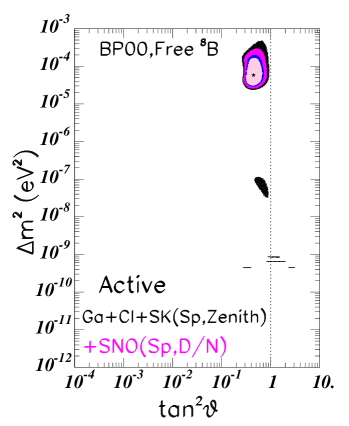
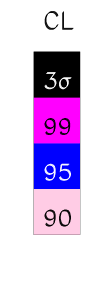
FIG. 1.: Allowed regions from the global fit for solar neutrino oscillations.

C The Future: KamLAND and Borexino

Our present understanding of the solar neutrino oscillation is being tested in the KamLAND experiment which is currently in operation in the Kamioka mine in Japan. This underground site is conveniently located at a distance of 150-210 km from several Japanese nuclear power stations. The measurement of the flux and energy spectrum of the $\bar{\nu}_{e}$’s emitted by these reactors will provide a test to the LMA solution of the solar neutrino anomaly [18].

After two or three years of data taking, KamLAND should be capable of either excluding the entire LMA region or, not only establishing $\nu_{e}\leftrightarrow\nu_{\rm other}$ oscillations, but also measuring the LMA oscillation parameters with unprecedented precision [20, 19, 39] provided that $\Delta m^{2}\leq{\rm few}10^{-4}$ eV². In Fig. 2 I show the expected precision in the construed oscillation parameters if KamLAND observes a signal corresponding to the expectations at the best fit point of the LMA region  [39]. KamLAND is expected to announce their first results this year. For the purpose of illustration I also show in Fig. 2 the results of a simulation of the expected accuracy with $\sim$ three months of data  [21].

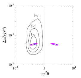
FIG. 2.: Left: Expected reconstructed regions (at 1, 2, and 3 $\sigma$ CL) if KamLAND observes a signal corresponding to the present best fit point of the LMA region. after three years of running. Right: Same but after three months of data taking (only the first octact in shown but the KamLAND regions are symmetric around maximal mixing since matter effects are negligible). The area to the right of the red curve will be ruled out if no oscillation signal is observed.

If LMA is confirmed, CP violation may be observable at future long-baseline (LBL) experiments. Also KamLAND will provide us, as data accumulate, with a firm determination of the corresponding oscillation parameters. With this at hand, the future solar $\nu$ experiments will be able to return to their original goal of testing solar physics.

If KamLAND does not confirm LMA, the next most relevant results will come from Borexino  [22]. The Borexino experiment is designed to detect low-energy solar neutrinos in real-time through the observation of the ES process $\nu_{a}+e^{-}\to\nu_{a}+e^{-}$. The energy threshold for the recoil electrons is 250 keV. The largest contribution to their expected event rate is from neutrinos of the ⁷Be line. Due to the lower energy threshold, Borexino is sensitive to matter effects in the Earth in the LOW region. And because ⁷Be neutrinos are almost monoenergetic, it is also very sensitive to seasonal variations associated with VAC oscillations.

III Atmospheric and Reactor Neutrinos

A The Evidence

Atmospheric showers are initiated when primary cosmic rays hit the Earth’s atmosphere. Secondary mesons produced in this collision, mostly pions and kaons, decay and give rise to electron and muon neutrino and anti-neutrinos fluxes whose interactions are detected in underground detectors [23, 24, 25, 27, 26]. Atmospheric neutrinos can be detected in underground detectors by direct observation of their charged current interaction inside the detector. These are the so called contained events. SK has divided their contained data sample into sub-GeV events with visible energy below 1.2 GeV and multi-GeV above such cutoff. On average, sub-GeV events arise from neutrinos of several hundreds of MeV while multi-GeV events are originated by neutrinos with energies of the order of several GeV. Higher energy muon neutrinos and antineutrinos can also be detected indirectly by observing the muons produced in their charged current interactions in the vicinity of the detector. These are the so called upgoing muons. Should the muon stop inside the detector, it will be classified as a “stopping” muon, (which arises from neutrinos of energies around ten GeV) while if the muon track crosses the full detector the event is classified as a “through-going” muon which is originated by neutrinos with energies of the order of hundred GeV.

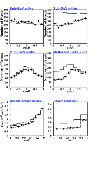
FIG. 3.: Zenith angle distribution of SuperKamiokande 1289 days data samples. Dots, solid line and dashed line correspond to data, MC with no oscillation and MC with best fit oscillation parameters, respectively. Allowed parameters from the global fit of atmospheric neutrino data for $\nu_{\mu}\rightarrow\nu_{\tau}$ oscillations.

At present the atmospheric neutrino anomaly (ANA) can be summarized in three observations (See Fig. 3):
– There has been a long-standing deficit of about 60 % between the predicted and observed $\nu_{\mu}$$/\nu_{e}$ ratio of the contained events strengthened by the high statistics sample collected at the SK experiment.
– The most important feature of the atmospheric neutrino data at SK is that it exhibits a zenith-angle-dependent deficit of muon neutrinos which indicates that the deficit is larger for muon neutrinos coming from below the horizon which have traveled longer distances before reaching the detector. On the contrary, electron neutrinos behave as expected in the SM.
– The deficit for through-going muons is smaller that for stopping muons, i.e. the deficit decreases as the neutrino energy grows.

B The Interpretation: Three-Neutrino Oscillations

The most likely solution of the ANA involves neutrino oscillations. At present the best solution from a global analysis of the atmospheric neutrino data is $\nu_{\mu}\rightarrow\nu_{\tau}$ oscillations with oscillation parameters shown in Fig. 4

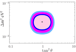
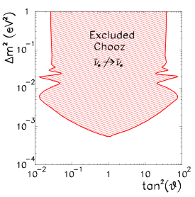
FIG. 4.: Left: Allowed parameters from the global fit of atmospheric neutrino data for $\nu_{\mu}\rightarrow\nu_{\tau}$ oscillations. Right: 90% CL excluded parameters by the CHOOZ experiment

Oscillations into electron neutrinos are nowadays ruled out since they cannot describe the measured angular dependence of muon-like contained events. Moreover the most favoured range of masses and mixings for this channel have been excluded by the negative results from the CHOOZ reactor experiment [28].

The CHOOZ experiment [28] searched for disappearance of $\bar{\nu}_{e}$ produced in a nuclear power station. At the detector, located at $L\simeq 1$ Km from the reactors, the $\bar{\nu}_{e}$ reaction signature is the delayed coincidence between the prompt ${\rm e^{+}}$ signal and the signal due to the neutron capture in the Gd-loaded scintillator. Their measured vs. expected ratio, averaged over the neutrino energy spectrum is

$$R=1.01\pm 2.8\,\%({\rm stat})\pm 2.7\,\%({\rm syst})\,.$$ (8)

Thus no evidence was found for a deficit of measured vs. expected neutrino interactions, and they derive from the data exclusion plots in the plane of the oscillation parameters in the simple two-neutrino oscillation scheme as shown Fig. 4.

Oscillations into sterile neutrinos are also disfavoured because due to matter effects in the Earth they predict a flatter-than-observed angular dependence of the through-going muon data [27].

The minimum joint description of atmospheric, solar and reactor data requires that all three known neutrinos take part in the oscillations. The mixing parameters are encoded in the $3\times 3$ lepton mixing matrix which can be conveniently parametrized in the standard form

$$U=\pmatrix{1&0&0\cr 0&{c_{23}}&{s_{23}}\cr 0&-{s_{23}}&{c_{23}}\cr}\pmatrix{{c_{13}}&0&{s_{13}}e^{i{\delta}}\cr 0&1&0\cr-{s_{13}}e^{-i{\delta}}&0&{c_{13}}\cr}\pmatrix{{c_{21}}&{s_{12}}&0\cr-{s_{12}}&{c_{12}}&0\cr 0&0&1\cr}$$ (9)

where $c_{ij}\equiv\cos\theta_{ij}$ and $s_{ij}\equiv\sin\theta_{ij}$. Notice that, since the two Majorana phases do not affect neutrino oscillations, they are not included in the expression above. The angles $\theta_{ij}$ can be taken without loss of generality to lie in the first quadrant, $\theta_{ij}\in[0,\pi/2]$. Concerning the CP violating phase $\delta$ we chose the convention $0\leq\delta\leq\pi$ and two choices of mass ordering.

For solar and atmospheric oscillations, the required mass differences satisfy

$$\Delta m^{2}_{\odot}=\Delta m^{2}\ll\Delta M^{2}=\Delta m^{2}_{\rm atm}.$$ (10)

so there are two possible mass orderings which, without any loss of generality can be chosen to be as shown in Fig. 5. The direct scheme is naturally related to hierarchical masses, $m_{1}\ll m_{2}\ll m_{3}$, for which $m_{2}\simeq\sqrt{\Delta m^{2}_{21}}$ and $m_{3}\simeq\sqrt{\Delta m^{2}_{32}}$ On the other hand, the inverted scheme implies that $m_{3}<m_{1}\simeq m_{2}$. In both cases neutrinos can have quasi-degenerate masses, $m_{1}\simeq m_{2}\simeq m_{3}\gg\Delta m^{2}_{21},|\Delta m^{2}_{32}|$. The two orderings are often referred to in terms of the sign($\Delta m^{2}_{31}$).

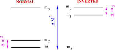
FIG. 5.: Mass schemes for 3 $\nu$ oscillations

Thus, in total the three-neutrino oscillation analysis involves seven parameters: 2 mass differences, 3 mixing angles, the CP phase and the sign($\Delta m^{2}_{31}$). In general the transition probabilities present an oscillatory behaviour with two oscillation lengths. For transitions in vacuum, the results for normal and inverted schemes are equivalent. In the presence of matter effects, this is no longer valid. However, the hierarchy in the splittings, Eq. (10), leads to important simplifications.
– For solar neutrinos the oscillations with the atmospheric oscillation length are averaged out and the survival probability takes the form:

$$P^{3\nu}_{ee,MSW}=\sin^{4}\theta_{13}+\cos^{4}\theta_{13}P^{2\nu}_{ee,MSW}$$ (11)

where $P^{2\nu}_{ee,MSW}$ is obtained with the modified sun density $N_{e}\rightarrow\cos^{2}\theta_{13}N_{e}$. So the analyses of solar data constrain three of the seven parameters: $\Delta m^{2}_{21},\theta_{12}$ and $\theta_{13}$. The effect of $\theta_{13}$ is to decrease the energy dependence of the solar survival probability.
– For atmospheric neutrinos, the solar wavelength is too long and the corresponding oscillating phase is negligible. As a consequence the atmospheric data analysis restricts $\Delta m^{2}_{31}\simeq\Delta m^{2}_{32}$, $\theta_{23}$ and $\theta_{13}$, the latter being the only parameter common to both solar and atmospheric neutrino oscillations and which may potentially allow for some mutual influence. The effect of $\theta_{13}$ is to add a $\nu_{\mu}\rightarrow\nu_{e}$ contribution to the atmospheric oscillations.
– At reactor experiments the solar wavelength is unobservable if $\Delta m^{2}<8\times 10^{-4}$ eV² and the relevant survival probability oscillates with wavelength determined by $\Delta m^{2}_{31}$ and amplitude determined by $\theta_{13}$.

CP is unobservable in the present data under the condition (10). There is, in principle some dependence on the normal versus inverted orderings due to matter effects in the Earth for atmospheric neutrinos, controlled by the mixing angle $\theta_{13}$. In Fig. 6 I show the allowed regions for the oscillation parameters $\Delta M^{2}$ and $\cos\delta\sin^{2}\theta_{23}$ from the analysis of the atmospheric neutrino data in the framework of three-neutrino oscillations  [29] for different values of $\sin^{2}\theta_{13}$. The figure illustrates how, under the condition (10), there is no dependence on the CP phase, $\delta$, while for large values of $\theta_{13}$ the results for normal and inverted schemes are different.

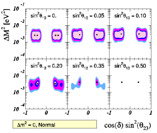
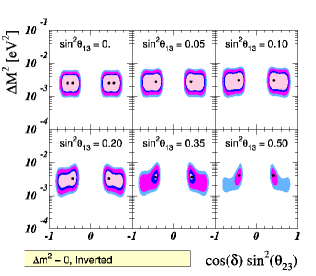
FIG. 6.: 90%, 95%, 99% and $3\sigma$ allowed regions in the $(\cos^{2}\delta\sin^{2}\theta_{23},\Delta M^{2})$ plane, for different values of $\sin^{2}\theta_{13}$ from the analysis of the atmospheric neutrino data.

From the analysis we also find that the atmospheric neutrino data favours $\theta_{13}$ small and an upper bound on this angle is obtained. This is due to the fact that the atmospheric data give no evidence for $\nu_{e}$ oscillation.

Actually all data independently favours $\theta_{13}=0$: the solar data exhibit energy dependence and this imposes a bound on $\theta_{13}$ although not very strict. Most important, reactor data exclude $\bar{\nu}_{e}$-disappearance’s at the atmospheric wavelength. In Fig. 7 I plot the results of the analysis of solar, atmospheric and reactor data on the allowed values of $\theta_{13}$.

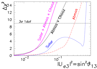
FIG. 7.: Dependence of $\Delta\chi^{2}$ on $\sin^{2}\theta_{13}$ in the analysis of the atmospheric, solar and CHOOZ neutrino data. The dotted horizontal line corresponds to the 3$\sigma$ limit for a single parameter.

The combined analysis results in a limit $\sin^{2}\theta_{13}\leq 0.06$ at 3$\sigma$ [29, 1]. Within this limit the difference between normal and inverted orderings in atmospheric neutrino data is below present experimental sensitivity. Thus, under the condition (10) the three-neutrino analysis of solar+atmospheric+reactor data effectively involves only five parameters.

The global analysis of solar, atmospheric and reactor data in the five-dimensional parameter space leads to the following allowed 3$\sigma$ ranges for individual parameters (that is, when the other four parameters have been chosen to minimize the global $\chi^{2}$):

$$2.4\times 10^{-5}< \Delta m^{2}_{21}/\mbox{\rm eV${}^{2}$} <2.4\times 10^{-4}\;\;\;\;\;{\rm LMA}\;$$ (12)

$$0.27< \tan^{2}\theta_{12} <0.77\;\;\;\;\;\;\;\;\;\;\;\;\;\;\;{\rm LMA}\;$$ (13)

$$1.4\times 10^{-3}< \Delta m^{2}_{32}/\mbox{\rm eV${}^{2}$} <6.0\times 10^{-3}$$ (14)

$$0.4< \tan^{2}\theta_{23} <3.0,$$ (15)

$$\sin^{2}\theta_{13} <0.06$$ (16)

These results can be translated into our present knowledge of the moduli of the mixing matrix $U$:

$$|U|=\pmatrix{0.73-0.89&0.45-0.66&<0.24\cr 0.23-0.66&0.24-0.75&0.52-0.87\cr 0.06-0.57&0.40-0.82&0.48-0.85\cr}.$$ (17)

C The Future: Long Baseline Experiments

$\nu_{\mu}$ oscillations with $\Delta m^{2}_{\rm atm}$ are being probed and will be further tested using accelerator beams at LBL experiments. In these experiments the intense neutrino beam from an accelerator is aimed at a detector located underground at a distance of several hundred kilometers. At present there are three such projects approved: K2K [30] which runs with a baseline of about 235 km from KEK to SK, MINOS [31] under construction with a baseline of 730 km from Fermilab to the Soudan mine where the detector will be placed, and two detectors, OPERA [32] and ICARUS [33] under construction with a baseline of 730 km from CERN to Gran Sasso.

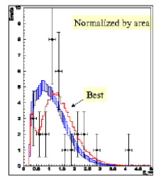
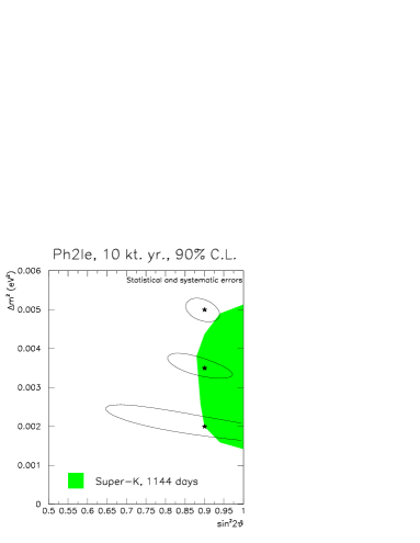
FIG. 8.: Left: Observed events at the K2K experiment, together with the expected distribution for the case of nooscillation and oscillations with the best fit point of the atmospheric neutrino analysis. Right: Expected reconstruction of the oscillation parameters in Minos.

The first results from K2K seem to confirm the atmospheric oscillations (see Fig 8) but statistically they are still not very significant. In the near future K2K will accumulate more data enabling it to confirm the atmospheric neutrino oscillation. Furthermore, combining the K2K and atmospheric neutrino data will lead to a better determination of the mass and mixing parameters.

In a longer time scale, the results from MINOS will provide more accurate determination of these parameters as shown in Fig. 8. OPERA and ICARUS are designed to observe the $\nu_{\tau}$ appearance. MINOS, OPERA and ICARUS have certain sensitivity to $\theta_{13}$ although by how much they will be ultimately able to improve the present bound is still undetermined.

IV LSND and Sterile Neutrinos

A The Evidence

The only positive signature of oscillations at a laboratory experiment comes from the Liquid Scintillator Neutrino Detector (LSND) which run at Los Alamos Meson Physics Facility. The primary neutrino flux comes from $\pi^{+}$’s produced in a 30-cm-long water target when hit by protons from the LAMPF linac with 800 MeV kinetic energy. Most of the produced $\pi^{+}$’s come to rest and decay through the sequence $\pi^{+}\to\mu^{+}\nu_{\mu}$, followed by $\mu^{+}\to e^{+}\nu_{e}\bar{\nu}_{\mu}$. The $\bar{\nu}_{\mu}$’s so produced have a maximum energy of $52.8$ MeV. This is called the decay at rest (DAR) flux and is used to study $\bar{\nu}_{\mu}\to\bar{\nu}_{e}$ oscillations. For DAR related measurements, $\bar{\nu}_{e}$’s are detected in the quasi elastic process $\bar{\nu}_{e}\,p\to e^{+}\,n$, in correlation with a monochromatic photon of $2.2$ MeV arising from the neutron capture reaction $np\to d\gamma$. Their final result is an excess of events of $87.9\pm 22.4\pm 6$ events, corresponding to an oscillation probability of $(2.64\pm 0.67\pm 0.45)\times 10^{-3}$.

B The Interpretation: Four Neutrino Mixing

In the two-family formalism the LSND results lead to the oscillation parameters shown in Fig. 9. The shaded regions are the 90 % and 99 % likelihood regions from LSND. The best fit point corresponds to $\Delta m^{2}=1.2$ eV² and $\sin^{2}2\theta=0.003$.

The region of parameter space which is favoured by the LSND observations has been partly tested by other experiments in particularly by the KARMEN experiment[35]. The KARMEN experiment was performed at the neutron spallation facility ISIS of the Rutherford Appleton Laboratory. They found no evidence of flavour transition which translated into exclusion curve in the two-neutrino parameter space given in Fig. 9

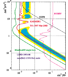
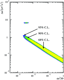
FIG. 9.: Left: Allowed regions (at 90 and 99 % CL) for $\bar{\nu}_{e}\to\bar{\nu}_{\mu}$ oscillations from the LSND experiment compared with the exclusion regions (at 90% CL) from KARMEN2 and other experiments. The 90 % CL expected sensitivity curve for MiniBooNE is also shown. Right: Allowed region from the combined analysis of LSND and KARMEN2 data.

Recently a combined analysis of the LSND and KARMEN data has been performed [36] which shows that both results can still be compatible within the parameter region shown in the left panel of Fig. 9.

To accommodate the LSND result together with the solar and atmospheric data in a single neutrino oscillation framework, there must be at least three different scales of neutrino mass-squared differences which requires the existence of a fourth light neutrino. The measurement of the decay width of the $Z^{0}$ boson into neutrinos makes the existence of three, and only three, light active neutrinos an experimental fact. Therefore, the fourth neutrino must not couple to the standard electroweak current, that is, it must be sterile.

One of the most important issues in the context of four-neutrino scenarios is the four-neutrino mass spectrum. There are six possible four-neutrino schemes, shown in Fig. 10, that can accommodate the results from solar and atmospheric neutrino experiments as well as the LSND result. They can be divided in two classes: (3+1) and (2+2). In the (3+1) schemes, there is a group of three close-by neutrino masses that is separated from the fourth one by a gap of the order of 1 eV², which is responsible for the SBL oscillations observed in the LSND experiment. In (2+2) schemes, there are two pairs of close masses separated by the LSND gap. The main difference between these two classes is the following: if a (2+2)-spectrum is realized in nature, the transition into the sterile neutrino is a solution of either the solar or the atmospheric neutrino problem, or the sterile neutrino takes part in both, whereas with a (3+1)-spectrum the sterile neutrino could be only slightly mixed with the active ones and mainly provide a description of the LSND result.

FIG. 10.: The six types of 4-neutrino mass spectra.

The phenomenological situation at present is that none of the four-neutrino scenarios are favoured by the data [40]. In brief (3+1)-spectra are disfavoured by the incompatibility between the LSND signal and the present constraints from short baseline laboratory experiments, while (2+2)-spectra are disfavoured by the existing constraints from the sterile oscillations in solar and atmospheric data.

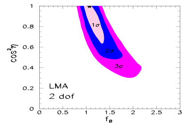
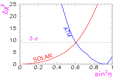
FIG. 11.: Left: Constraint on the active-sterile admixture in solar neutrino oscillations versus the ⁸B neutrino flux enhancement factor. Right: Present status of the bounds on the active-sterile admixture from solar and atmospheric neutrino data in (2+2)-models.

In this respect it has been recently pointed out that the existing constraint on the sterile admixture in the solar neutrino oscillations can be relaxed if the ⁸B neutrino flux is allowed to be larger than in the SSM by a factor $f_{B}$ [38, 39]. The analysis is performed in the context of solar conversion $\nu_{e}\rightarrow\nu_{x}$, where $\nu_{x}=\cos\eta~{}\nu_{a}+\sin\eta~{}\nu_{s}$. In Fig. 11 I show the presently allowed range of $\eta$ as a function of $f_{B}$. The obtained upper bound on $\sin^{2}\eta$ from this most general solar analysis has to be compared with the corresponding lower bound from the analysis of atmospheric data. In Fig. 11 I show the corresponding comparison (the curve for the atmospheric data is taken from Ref. [40]).

C The Future: MiniBooNE

The MiniBooNE experiment [37], will be able to confirm or disprove the LSND oscillation signal within the next two years (see Fig. 9). Should the oscillation signal be confirmed as well as the solar signal in KamLAND and the atmospheric in LBL experiments, we will face the challenging situation of not having a successful “minimal” phenomenological description at low-energy of the leptonic mixing.

Alternative explanations to the LSND observation include the possibility of CPT violation [41] which would imply that the mass differences and mixing among neutrinos would be different from the ones for antineutrinos. This scenario is being tested with the running experiments. An imminent test of CPT will be the comparison of the observation in KamLAND of $\overline{\nu_{e}}$ disappearance versus solar $\nu_{e}$ disappearance. Also, at present, MiniBooNE [37] is running in the neutrino mode searching for $\nu_{\mu}\rightarrow\nu_{e}$ to be compared with the antineutrino signal in LSND. Thus an oscillation signal at KamLAND or MiniBooNE will put serious constraints on CPT violation for $\nu$’s.

V Neutrino Mass Scale

Oscillation experiments provide information on $\Delta m^{2}_{ij}$, and on the leptonic mixing angles, $U_{ij}$. But they are insensitive to the absolute mass scale for the neutrinos. Of course, the results of an oscillation experiment do provide a lower bound on the heavier mass in $\Delta m^{2}_{ij}$, $|m_{i}|\geq\sqrt{\Delta m^{2}_{ij}}$ for $\Delta m^{2}_{ij}>0$. But there is no upper bound on this mass. In particular, the corresponding neutrinos could be approximately degenerate at a mass scale that is much higher than $\sqrt{\Delta m^{2}_{ij}}$. Moreover, there is neither upper nor lower bound on the lighter mass $m_{j}$.

Information on the neutrino masses, rather than mass differences, can be extracted from kinematic studies of reactions in which a neutrino or an anti-neutrino is involved. In the presence of mixing the most relevant constraint comes from Tritium beta decay ${\rm{}^{3}H\rightarrow\ ^{3}He+e^{-}+\overline{\nu}_{e}}$ which, within the present and expected experimental accuracy, can limit the combination

$$m_{\beta}=\sum_{i}m_{i}|U_{ei}|^{2}$$ (18)

The present bound is $m_{\beta}\leq 2.2$ eV at 95 % CL [42]. A new experimental project, KATRIN, is under consideration with an estimated sensitivity limit: $m_{\beta}\sim 0.3$ eV.

Direct information on neutrino masses can also be obtained from neutrinoless double beta decay $(A,Z)\rightarrow(A,Z+2)+e^{-}+e^{-}$. The rate of this process is proportional to the effective Majorana mass of $\nu_{e}$,

$$m_{ee}=\left|\ \ \sum_{i}m_{i}U_{ei}^{2}\ \ \right|$$ (19)

which, unlike Eq. (18), depends also on the three CP violating phases. Notice that in order to induce the $2\beta 0\nu$ decay, $\nu$’s must Majorana particles.

The present strongest bound from $2\beta 0\nu$-decay is $m_{ee}<0.34$ eV at 90 % CL [43]. Taking into account systematic errors related to nuclear matrix elements, the bound may be weaker by a factor of about 3. A sensitivity of $m_{ee}\sim 0.1$ eV is expected to be reached by the currently running NEMO3 experiment, while a series of new experiments is planned with sensitivity of up to $m_{ee}\sim 0.01$ eV [45] (see Table II for some of these proposals).

Experiment	Search	Source	goal
KATRIN	3H $\beta$-dec		${m_{\beta}}<0.3$– 0.4 eV
NEMO3	$(\beta\beta)_{0\nu}$	100Mo	$|\langle m_{ee}\rangle|\sim 0.2$ eV
CUORE	$(\beta\beta)_{0\nu}$	130Te	$|\langle m_{ee}\rangle|\sim 0.03$ eV
EXO	$(\beta\beta)_{0\nu}$	136Xe	$|\langle m_{ee}\rangle|\sim 0.05$ eV
MOON	$(\beta\beta)_{0\nu}$	100Mo	$|\langle m_{ee}\rangle|\sim 0.04$ eV
GENIUS	$(\beta\beta)_{0\nu}$	76Ge	$|\langle m_{ee}\rangle|\sim 0.01$ eV
Majorana	$(\beta\beta)_{0\nu}$	76Ge	$|\langle m_{ee}\rangle|\sim 0.02$ eV

TABLE II.: Future experiments and their proposed sensitivity to the relevant neutrino mass scale.

The knowledge of $m_{ee}$ can provide information on the mass and mixing parameters that is independent of the $\Delta m^{2}_{ij}$’s. However, to infer the values of neutrino masses, additional assumptions are required. In particular, the mixing elements are complex and may lead to strong cancellation, $m_{ee}\ll m_{1}$. Yet, the combination of results from $2\beta 0\nu$ decays and Tritium beta decay can test and, in some cases, determine the mass parameters of given schemes of neutrino masses [44] provided that the nuclear matrix elements are known to good enough precision. This work is supported by the MC fellowship HPMF-CT-2000-00516 and by the Spanish DGICYT grant FPA2001-3031.

REFERENCES

- [1] For a recent review on the status of neutrino masses and mixing, see M.C. Gonzalez-Garcia and Y. Nir, hep-ph/0202058, Rev. Mod. Phys, in press.
- [2] Kobayashi, M., and T. Maskawa,, Prog. Theor. Phys. 49, 652 (1973).
- [3] Z. Maki, M. Nakagawa, and S. Sakata, Prog. Theor. Phys. 28, 870 (1962).
- [4] B. Pontecorvo, J. Exptl. Theoret. Phys. 33, 549 (1957).
- [5] L. Wolfenstein, Phys. Rev. D 17, 2369 (1978); S.P. Mikheyev, and A.Y. Smirnov, Yad. Fiz. 42, 1441 (1985) [Sov. J. Nucl. Phys. 42, 913].
- [6] A. de Gouvea, A. Friedland and H. Murayama, Phys. Lett. B 490, 125 (2000); M. C. Gonzalez-Garcia, C. Peña-Garay, Phys. Rev. D62, 031301 (2000); G. L. Fogli, E. Lisi, A. Maronne and G. Scioscia, Phys. Rev. D59, 033001 (1999); C. Giunti, M. C. Gonzalez-Garcia, C. Peña-Garay, Phys. Rev. D62, 013005 (2000).
- [7] B.T. Cleveland et al., Astrophys. J. 496, 505 (1998).
- [8] GALLEX Coll. , W. Hampel et al., Phys. Lett. B 447, 127 (1999).
- [9] GNO Coll., M. Altmann et al., Phys. Lett.B 490, 16 (2000.
- [10] SAGE Coll., J.N. Abdurashitov et al., J. Exp. Theor. Phys. 95, 181 (2002).
- [11] Kamiokande Coll., Y. Fukuda et al., Phys. Rev. Lett. 77, 1683 (1996).
- [12] Super-Kamiokande Coll., S. Fukuda et al., Phys. Lett. B 539, 179 (2002).
- [13] J.N. Bahcall, H.M. Pinsonneault, and S. Basu, Astrophys. J. 555, 990 (2001).
- [14] SNO Coll., Q.R. Ahmad et al. Phys. Rev. Lett. 87, 071301 (2001).
- [15] SNO Coll., Q.R. Ahmad et al. Phys. Rev. Lett. 89, 011301 (2002); ibid 011302.
- [16] SNO coll., nucl-ex/0204009; Barger et al., hep-ph/0204253; Bandyopadhysy et al, hep-ph/0204286; Bahcall et al, hep-ph/0204314; Creminelli et al, hep-ph/0102234; Aliani et al hep-ph/0205053; de Holanda, Smirnov, hep-ph/0205241; Strumia et al, hep-ph/0205262; Fogli et al, hep-ph/0206162; Maltoni et al,hep-ph/0207227.
- [17] J.N. Bahcall, M.C. Gonzalez-Garcia, C. Peña-Garay, JHEP 0207, 054 (2002).
- [18] Piepke, A. et al., 2001, Nucl. Phys. Proc. Suppl. 91, 99.
- [19] V. D. Barger, D. Marfatia and B. P. Wood, Phys. Lett. B 498, 53 (2001); A. de Gouvêa and C. Peña-Garay, Phys. Rev. D 64, 113011 (2001)
- [20] H. Murayama and A. Pierce, Phys. Rev. D 65, 013012 (2002)
- [21] C. Peña-Garay, private communication.
- [22] L. Oberauer, Nucl. Phys. Proc. Suppl. 77, 48 (1999).
- [23] IMB Coll., R. Becker-Szendy, et al., Phys. Rev. D 46, 3720 (1992).
- [24] Kamiokande Coll., Y. Fukuda, et al., Phys. Lett. B 335, 237 (1994).
- [25] Soudan Coll., W.W.M. Allison ,et al., Phys. Lett. B 449, 137 (1999).
- [26] MACRO Coll., M. Ambrosio, et al., Phys. Lett. B 517, 59 (2001).
- [27] Super-Kamiokande Coll., Y. Fukuda et al., Phys. Lett. B433, 9 (1998) .
- [28] CHOOZ Collaboration, M. Apollonio et al., Phys.Lett. B420, 397 (1998).
- [29] M. C. Gonzalez-Garcia and M. Maltoni, hep-ph/0202218.
- [30] S.H. Ahn , et al., K2K Coll., Phys. Lett. B 511, 178 (2001).
- [31] S.G. Wojcicki, Nucl. Phys. Proc. Suppl. 91, 216 (2001).
- [32] A.G. Cocco, et al., OPERA Coll., Nucl. Phys. Proc. Suppl. 85, 125 (2000).
- [33] O. Palamara, et al., ICARUS Coll,, Nucl. Phys. Proc. Suppl. 110, 329 (2002).
- [34] LSND Coll., C. Athanassopoulos, et al., Phys. Rev. Lett. 81, 1774 (1998) 1774.
- [35] M. Steidl KARMEN Coll., Nucl. Phys. Proc. Suppl. 110 (2002) 417.
- [36] E. D. Church, K. Eitel, G. B. Mills and M. Steidl, Phys. Rev. D 66, 013001 (2002)
- [37] A. Bazarko, et al., MiniBooNE Collaboration, Nucl. Phys. Proc. Suppl. 91, 210 (2000).
- [38] V. Barger, D. Marfatia, and K. Whisnant, Phys. Rev. Lett. 88, 011302 (2002)
- [39] J. N. Bahcall, M. C. Gonzalez-Garcia and C. Pena-Garay, Phys. Rev. C 66, 035802 (2002).
- [40] Maltoni, M., M.A. Tortola, T. Schwetz and J.W. Valle, 2002, hep-ph/0207227.
- [41] H. Murayama, and T. Yanagida, , Phys. Lett. B 520, 263 (2001); S. Pakvasa, hep-ph/0110175; G. Barenboim et al., hep-ph/0108199; Skadghauge, hep-ph/0112189; A. Strumia, hep-ph/0201134.
- [42] J. Bonn, et al., Nucl. Phys. Proc. Suppl. 91, 273 (2001); V.M. Lobashev, et al., Nucl. Phys. Proc. Suppl. 91, 280 (2001).
- [43] H.V. Klapdor-Kleingrothaus, H.V., Eur. Phys. J. A 12 147 (2001).
- [44] F. Vissani, JHEP 9906, 022 (1999); Y. Farzan, O. L. Peres and A. Y. Smirnov, Nucl. Phys. B 612, 59 (2001); S.M. Bilenky, S.M., S. Pascoli and S. T. Petcov, Phys. Rev. D 64, 053010 (2001); ibid 113003;S. Pascoli, and T.S. Petcov hep-ph/0205022.
- [45] S. R. Elliott and P. Vogel, hep-ph/0202264; O. Cremonesi, hep-ex/0210007.