Two Loop Electroweak Bosonic Corrections to the Muon Decay Lifetime

Abstract

A review of the calculation of the two loop bosonic corrections to $\Delta r$ is presented. Factorization and matching onto the Fermi model are discussed. An approximate formula, describing the quantity over the interesting range of Higgs boson mass values from 100 GeV to 1 TeV is given.

The muon decay lifetime ($\tau_{\mu}$) has been used for long as an input parameter for high precision predictions of the Standard Model (SM). It allows for an indirect determination of the mass of the $W$ boson ($M_{W}$), which suffers currently from a large experimental error of 33 MeV [1], one order of magnitude worse than that of the $Z$ boson mass ($M_{Z}$). A reduction of this error by LHC to 15 MeV [2] and by a future linear collider to 6 MeV [3] would provide a stringent test of the SM by confronting the theoretical prediction with the experimental value.

The extraction of $M_{W}$ with an accuracy matching that of next experiments, i.e. at the level of a few MeV necessitates radiative corrections beyond one loop order. Large two loop contributions from fermionic loops have been calculated in [4]. The current prediction is affected by two types of uncertainties. First, apart from the still unknown Higgs boson mass, two input parameters introduce large errors. The current knowledge of the top quark mass results in an error of about 30 MeV [5], which should be reduced by LHC to 10 MeV and by a linear collider even down to 1.2 MeV. The inaccuracy of the knowledge of the running of the fine structure constant up to the $M_{Z}$ scale, $\Delta\alpha(M_{Z})$, introduces a further $6.5$ MeV error. Second, several higher order corrections are unknown. In fact the last correction of order ${\cal O}(\alpha^{2})$, generated by purely electroweak bosonic loops, has been calculated only recently in [6] and confirmed by an independent group in [7]. The details of both calculations are presented in [8].

The two loop bosonic corrections to the muon lifetime have been previously estimated by two different methods. First, the leading term in the large Higgs boson mass expansion has been obtained in [9] and [10]. Although the results were different, the size of the contributions was negligible. Apart from the disagreement, the large mass expansion is not justified for small Higgs boson masses, and the experimental data seems to favour a low mass range. Second, a resummation formula has been used [5], which with respect to bosonic corrections consists of assuming a geometric progression of the contributions with the order of perturbation theory. This means that at two loop order, the bosonic corrections should be equal to the square of the one loop result. This, however, is contradicted by the fact, that the leading behaviour with the Higgs boson mass would then be of logarithmic type ($\sim\log^{2}(M_{H}^{2})$), whereas it is known that the result should behave as the square of this mass [11].

Since both estimates turn out to be unreliable the full calculation was necessary. Here we shall describe the crucial ingredients, starting from the proper definition of $\Delta r$, passing through the various stages of the renormalization procedure, and ending with the methods used in numerical evaluation.

The muon decay is described by an effective field theory, the Fermi model, which consists of $QED$, $QCD$ of five light quarks and the four fermion point interaction

$${\cal L}_{F}=\frac{G_{F}}{\sqrt{2}}\bar{e}\gamma^{\alpha}(1-\gamma_{5})\mu\otimes\bar{\nu_{\mu}}\gamma_{\alpha}(1-\gamma_{5})\nu_{e}.$$ (1)

The constant $G_{F}$ should be predicted by the Standard Model. The difference between the tree level prediction and the full result is factorized in the quantity $\Delta r$

$$\frac{G_{F}}{\sqrt{2}}=\frac{\pi\alpha}{2M_{W}^{2}s_{W}^{2}}(1+\Delta r).$$ (2)

In this sense $\Delta r$ can be considered as the matching or Wilson coefficient in the Fermi model. The matching equation assumes the form

$$S^{\rm SM}=S^{\rm Fermi}+{\cal O}\left(\frac{p^{4}}{M_{W}^{4}},\frac{m^{4}}{M_{W}^{4}}\right),$$ (3)

where $p$ and $m$ denote the external momenta and the light masses respectively, and $S$ is the renormalized scattering matrix in both models. The easiest way to obtain $\Delta r$ is to simply put $p$ and $m$ equal to zero on both sides of the equation. This procedure will of course generate spurious infrared divergences, which however will cancel from the equation as has been shown in [12]. The main advantage comes from the fact, that on the right side, all loop diagrams will be scaleless (as they contain only light particles), and will therefore vanish, leaving only the tree level diagram trivially proportional to $G_{F}$. Additionally, the SM diagrams on the left hand side will reduce to vacuum bubbles.

A major point in the above procedure is connected with the treatement of spinor chains. Dimensional regularization for spurious infrared divergencies forbids a direct use of the Chisholm identity

$$\gamma_{\mu}\gamma_{\nu}\gamma_{\rho}=g_{\mu\nu}\gamma_{\rho}+g_{\nu\rho}\gamma_{\mu}-g_{\mu\rho}\gamma_{\nu}-i\epsilon_{\mu\nu\rho\sigma}\gamma^{\sigma}\gamma_{5}$$ (4)

for all diagrams, which are divergent after renormalization. A priori we would have to introduce a whole basis of tensor products of possible spinor chains. It turns out, however, that the projection onto the Fermi operator can be defined unambiguously through Fierz symmetry. The problematic diagrams contain always a photon line connecting the two chains. A Fierz rearrangement about this line or the $W$ boson line, as depicted in Fig. 1, leads to an object which has the required vertex structure

$$\gamma^{\mu}P_{L}\otimes\gamma_{\mu}P_{L}.$$ (5)

In practice, this Fierz rearrangement can be realised with the help of a projector. In the present case, the transformation

$$\Gamma_{1}\otimes\Gamma_{2}\rightarrow-\frac{1}{2D(D-2)}\mbox{Tr}(\Gamma_{1}\gamma_{\mu}P_{R}\Gamma_{2}\gamma^{\mu}P_{R})$$ (6)

gives directly the coefficient of the operator Eq. 5 in $D$ dimensions.

Figure 1: Example of a Fierz rearrangement about the photon line.

The matching procedure requires proper renormalization of the model. Although in the end we are interested in the on-shell parametrization for the masses and the electric charge, an intermediate renormalization can be chosen at will. In fact the factorization theorem [12] has been proven for mass independent schemes and the on-shell scheme does not have this property. However, as long as the parameters are defined at the heavy scale the mass dependence does not contradict the theorem. For this reason, we may safely renormalize the boson masses in the on-shell scheme. The situation is somewhat more problematic with the electric charge, which is usually defined by the Thompson scattering processes for on shell electrons and photon. If we are interested in bosonic corrections only, the definition can be kept, since an inspection of the diagrams leads to the conclusion that no spurious infrared divergencies can be introduced. For light fermionic contributions the situation is different with the usual solution consiting of a shift of the definition to the $M_{Z}$ scale [13].

In this work, two renormalisation schemes have been used. First, the complete calculation has been performed in the on-shell scheme. Second, the model has been renormalized in the $\overline{\rm MS}$ scheme, and the result translated back to the on-shell scheme by means of relations between the on-shell and $\overline{\rm MS}$ masses, which for the $W$ and $Z$ masses were required up to two loop order. Obviously the translation should be applied to a scheme independent quantity. In this case, this is the Fermi constant $G_{F}$, and the correct relation is

$$\left.\frac{\pi\alpha}{2M_{W}^{2}s_{W}^{2}}(1+\Delta r)\right|_{\rm OS}=\left.\frac{\pi\alpha}{2M_{W}^{2}s_{W}^{2}}(1+\Delta r)\right|_{\overline{\rm MS}}.$$ (7)

It is not trivial that the formulae will coincide, since the on-shell counterterms on the left hand side contain terms of order $\epsilon$ ($\epsilon=1/2(4-D)$), which are not used in the translation between the schemes on the right hand side.

An interesting part of the definition of the model is the treatement of tadpole diagrams. It is known that gauge invariance of mass counter-terms requires inclusion of tadpoles [14, 15] (at the two loop level this has been explicitely shown in [16]). In this case, however, one cannot use one-particle-irreducible (1PI) Green functions. In order to have gauge invariant counter-terms and 1PI Green functions only, a special procedure was designed. An additional renormalisation constant for the bare vacuum expectation value $v_{0}$, denoted $Z_{v}$, has been introduced and explicitely split from the bare masses

$$v_{0} \longrightarrow v_{0}Z_{v}^{1/2},$$ (8)

$$M^{0}_{W,Z} \longrightarrow M^{0}_{W,Z}Z_{v}^{1/2}.$$ (9)

The term linear in the Higgs field $H$ in the lagrangian

$$T^{0}H^{0}=\frac{M^{0}_{W}s^{0}_{W}}{e_{0}}(M^{0}_{H})^{2}Z_{v}^{1/2}(Z_{v}-1)H^{0},$$ (10)

is then used to determine $Z_{v}$, through the requirement that tadpoles are canceled. It can be proved [8, 14] that the bare masses are gauge invariant in this case.

It should be stressed that this procedure can be advantageous at higher orders, since the number of diagrams is strongly reduced by using 1PI Green functions. For the muon decay, there are twice as many diagrams if tadpoles are introduced. If a treatement per diagram is required (e.g. expansion), the calculation time is strongly correlated to the number of diagrams and substantial differences in execution can be observed.

Having defined the method of factorization and renormalization, we turn to the calculation of the respective diagrams. As noticed already above, all of the bare diagrams are of the vacuum type, and for these a reduction procedure supplied with analytical formulae is known [17]. The situation is slightly more complicated with the on-shell two point functions that are needed for the on-shell definition of masses. The strategy adopted in this work consists of two algorithms. The first one [18] reduces the tensor integrals to scalar ones and uses topological symmetries to lead to as small a set of basic integrals as possible. The integrals obtained in this way are now subject to numerical evaluation. We used the efficient one dimensional representation given in [19] and extended its implementation (S2LSE) to work with software emulated quadruple precision.

Several tests have been applied to the numerics. First of all, the $Z$ boson propagator has been completely tested by means of the low momentum expansion, which is valid in this case, as all diagrams are below threshold. A 6 digit coincidence has been found at tenth order. The $W$ propagator required the use of large mass expansions, since several diagrams are at threshold, but the same precision as previously was also obtainable. Finally both propagators were tested against the result for the $\overline{\rm MS}$ to on-shell mass relations of the two gauge bosons given in [16]. This was also considered as a test of the gauge invariance of the mass counterterms.

Concerning gauge invariance, all of the calculations apart from the two two loop mass counterterms, have been performed in the general $R_{\xi}$ gauge with three parameters and the cancellation of the dependence on these parameters has been explicitely verified.

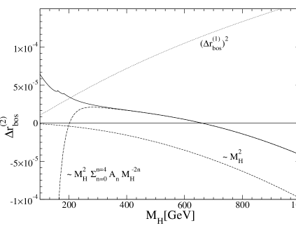
Figure 2: The full result for the bosonic corrections to $\Delta r$ (solid line) against the large mass expansion with leading term and the square of the one loop result.

The full result is given in Fig. 2 as function of the Higgs boson mass, for the following values of the input parameters

$$\alpha^{-1}=137.03599976,$$ (11)

$$M_{W}=80.423\mbox{ GeV},$$

$$M_{Z}=91.1876\mbox{ GeV}.$$

On the same plot, the leading term of the large Higgs boson mass expansion [6, 9] and the square of the one loop result are shown to contrast the previous estimates with the full result.

Our result has also been reexpanded in the large Higgs boson mass for comparison with [7] using the $\overline{MS}$ value and the expansion of the translation formulae given in [16]. The five term expansion is also shown in Fig. 2.

It turns out that the variation of the result with the $W$ mass within the experimental error bars of $\pm 33$ MeV [1] is negligible. The correction can be described to $5\%$ accuracy outside of the double threshold region for Higgs boson masses ranging from 100 GeV to 1 TeV, with the following formula

$$a+b\Delta+c_{1}L+c_{2}L^{2},$$ (12)

where

$$\Delta=\left(\frac{M_{H}}{100\;\mbox{GeV}}\right)^{2}-1,$$ (13)

$$L=\log\left[\left(\frac{M_{H}}{100\;\mbox{GeV}}\right)^{2}\right],$$ (14)

and the coefficients are

$$a = 6.385\times 10^{-5},$$

$$b = -1.110\times 10^{-6},$$

$$c_{1} = -2.870\times 10^{-5},$$

$$c_{2} = 6.445\times 10^{-6}.$$ (15)

The effect on the prediction of the $W$ boson mass from the muon decay lifetime is small and can be obtained from an expansion. In fact $6\%$ accuracy is guaranteed by estimating the resulting mass shift from the formula

$$\Delta M_{W}=-1.491\times 10^{4}\Delta r^{(2)}_{bos}\mbox{ [MeV]}.$$ (16)

The respective plot is shown in Fig. 3.

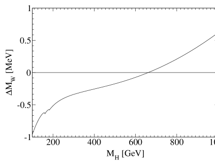
Figure 3: $W$ boson mass shift generated by two loop bosonic corrections.

In conclusion, the calculation of the two loop bosonic corrections to the muon decay lifetime as parametrized by $\Delta r$ has been reviewed. The crucial steps of the factorization and matching have been described together. A simple formula describing the correction for a large range of Higgs boson masses has been given.

M. C. would like to thank the Alexander von Humboldt foundation for fellowship. This work was supported in part by the European Community’s Human Potential Programme under contract HPRN-CT-2000-00149 Physics at Colliders, and by the KBN Grants 5P03B09320 and 2P03B05418.

References

- [1] C. J. Parkes [LEP Collaborations], arXiv:hep-ex/0205086.
- [2] ATLAS Collaboration, CERN/LHCC/99-15 (1999); CMS Collaboration, CMS TDR 1–5 (1997/98); S. Haywood et al., hep-ph/0003275.
- [3] TESLA Technical Design Report, Part III, eds. R. Heuer, D. J. Miller, F. Richard and P. M. Zerwas, DESY-2001-11C, hep-ph/0106315; T. Abe et al., arXiv:hep-ex/0106057.
- [4] G. Degrassi, P. Gambino and A. Vicini, Phys. Lett. B 383 (1996) 219; G. Degrassi, P. Gambino and A. Sirlin, Phys. Lett. B 394 (1997) 188; A. Freitas, W. Hollik, W. Walter and G. Weiglein, Phys. Lett. B 495 (2000) 338.
- [5] A. Freitas, W. Hollik, W. Walter and G. Weiglein, Nucl. Phys. B 632 (2002) 189.
- [6] M. Awramik and M. Czakon, arXiv:hep-ph/0208113, to appear in Phys. Rev. Lett.
- [7] A. Onishchenko and O. Veretin, arXiv:hep-ph/0209010.
- [8] M. Awramik, M. Czakon, A. Onishchenko and O. Veretin, arXiv:hep-ph/0209084.
- [9] F. Halzen, B. A. Kniehl and M. L. Stong, Z. Phys. C 58 (1993) 119.
- [10] F. Jegerlehner, Prog. Part. Nucl. Phys. 27 (1991) 1.
- [11] M. J. Veltman, Acta Phys. Polon. B 8 (1977) 475.
- [12] S. G. Gorishnii, Nucl. Phys. B 319 (1989) 633.
- [13] A. Sirlin, Phys. Rev. D 22 (1980) 971.
- [14] T. Appelquist, J. Carazzone, T. Goldman and H. R. Quinn, Phys. Rev. D 8 (1973) 1747.
- [15] J. C. Taylor, “Gauge Theories Of Weak Interactions”, Cambridge 1976, 167p; J. Fleischer and F. Jegerlehner, Phys. Rev. D 23 (1981) 2001.
- [16] F. Jegerlehner, M. Y. Kalmykov and O. Veretin, Nucl. Phys. B 641 (2002) 285.
- [17] A. I. Davydychev and J. B. Tausk, Nucl. Phys. B 397 (1993) 123.
- [18] G. Weiglein, R. Scharf and M. Bohm, Nucl. Phys. B 416 (1994) 606.
- [19] S. Bauberger, F. A. Berends, M. Bohm and M. Buza, Nucl. Phys. B 434 (1995) 383.