Measurement of the Muon Anomalous Magnetic Moment to 0.7 ppm [1]

Abstract

The experimental method together with the analysis method and results of the data taken in 2000 and prospects of the muon anomalous magnetic and electric dipole moment experiments are presented here.

1 Introduction

The $g$ factor of a particle, defined as the ratio of the magnetic moment of the particle in units of its Bohr magneton, over the angular momentum of the same particle in units of $\hbar$:

$$g={{\rm magnetic\,\,moment\over e\hbar/2mc}\over{\rm angular\,\,moment\over\hbar}},$$ (1)

is used to enhance our understanding of the underlying theory, like:

1. It is used to indicate that the proton ($g_{p}=+5.586$) and the neutron ($g_{n}=-3.826$) are composite particles.

2. The ratio $g_{p}/g_{n}$ of -1.46 being close to the predicted -3/2 was the first success of the constituent quark model.

3. The g-2 value of the electron is non-zero due to quantum field fluctuations. The agreement between the experimental and the theoretical value is a triumph of both QED and of the experimental approach.

4. The g-2 value of the muon is usually more sensitive to higher mass particles than the electron g-2 by the ratio of $(m_{\mu}/m_{e})^{2}\approx 40000$. Therefore it is used widely to check the validity of the standard model and as a sensitive probe for physics beyond it.

2 Theory

The anomalous magnetic moment of the muon, defined as $a_{\mu}={g_{\mu}-2\over 2}$, is the sum of QED, hadronic, and weak interaction contributions plus any new physics that may be present:

$$a_{\mu}({\rm theo}) = a_{\mu}({\rm QED})+a_{\mu}({\rm had})+a_{\mu}({\rm weak})+$$ (2)

$$a_{\mu}({\rm new\,\,physics}).$$

The theoretical values of the various contributions, especially that of the hadronic one, are the subject of many papers [3, 4, 5, 6, 7, 8, 9, 10]:

• $a_{\mu}({\rm QED})=11\,658\,470.57(0.29)\times 10^{-10}\,\,(0.025\,\rm ppm)$  [13].

• $a_{\mu}({\rm had})=683.3(7.7)\times 10^{-10}\,\,(0.66\,\rm ppm)$, based on the $e^{+}e^{-}$ value for the lowest-order hadronic correction of $a_{\mu}({\rm had,1})=684.7(7.0)\times 10^{-10}\,\,(0.60\,\rm ppm)$ [9] since only these data can be directly related to $a_{\mu}({\rm had})$ without further theoretical assumptions. The higher-order hadronic contribution of $a_{\mu}({\rm had,2})=-10.0(0.6)\times 10^{-10}$ [11], and $a_{\mu}({\rm had,lbl})=8.6(3.2)\times 10^{-10}$ [12]. For completeness $a_{\mu}({\rm had,1})=701.9(6.2)\times 10^{-10}\,\,(0.53\,\rm ppm)$ based on the $\tau$ data [9].

• $a_{\mu}({\rm weak})=15.1(0.4)\times 10^{-10}\,\,(0.03\,\rm ppm)$ [10].

Then the standard model contribution $a_{\mu}({\rm SM})=11\,659\,169(7.7)\times 10^{-10}$ with a relative uncertainty of $(0.66\,\rm ppm)$. The Feynman diagrams of the second order weak contributions are shown in Figure (1). An example of $a_{\mu}({\rm new\,\,physics})$ is the contribution due to SUSY, Figure (2), where the supersymmetric partners of $W$ and $Z$, the chargino and neutralino, are involved. Their contribution is estimated to be

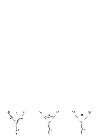
Figure 1: Second order weak contributions to $a_{\mu}$ involving the $W$, $Z$, and Higgs. The Higgs contribution is negligible for the present mass limits. The total relative weak contribution is estimated to be +1.3 ppm with an error of 0.03 ppm.

$$a_{\mu}({\rm SUSY})=14\times 10^{-10}\left({100\rm GeV\over m_{\rm susy}}\right)^{2}\,\tan{\beta}.$$ (3)

Figure 2: SUSY contributions to $a_{\mu}$ involving the superpartners of $W$, and $Z$. Their contribution, enhanced by the factor $\tan{\beta}$, may be larger than the weak.

3 Experimental Method

A bunch of highly polarized muons with momentum $P\approx 3.09\,{\rm GeV/}c$ is injected into a ring of 7.112 m radius, Figure (3), with 1.45 T dipole magnetic field of very high uniformity. The time distribution of the injected beam has an r.m.s. of 25 ns. At $\approx 90^{\circ}$ from the injection point, the muon beam is kicked onto stable orbits by a fast magnetic pulse (kicker) [14]. Within a super-cycle of 3.2 s there are 12 bunches, 33 ms apart from each other. Vertical focusing is provided by electrostatic quadrupoles [15]. Muons of that momentum have a lifetime of $\gamma\tau_{\mu}\approx 64.4\,\rm\mu s$ and are stored in the ring for $\approx 1.4$ ms.

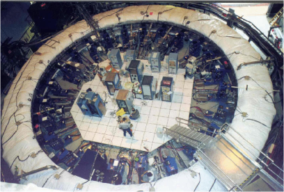
Figure 3: The g-2 muon storage ring is shown here with the thermal isolation cover (white) in place.

3.1 Principle of the g-2 Experiment

The muon momentum vector in the lab frame, $\vec{P}$, precesses under the influence of the electromagnetic forces. The muon spin in its own rest frame, $\vec{S}$, precesses under the influence of only the magnetic forces present in its rest frame. Muon decay violates parity in a maximal way; in the muon rest frame the most energetic electrons go along the muon spin direction. Then the energy of the electron is Lorentz boosted due to the muon momentum resulting in an energy which is modulated according to the dot product of the two vectors [16, 17], $\vec{S}\cdot\vec{P}$, which for a spin 1/2 particle is an exact sine wave of angular frequency $\omega_{a}$, giving rise to the principle of g-2 frequency detection.

The electrons, having on average less momentum than the stored muons, spiral inwards where they are collected by an inner ring of 24 electromagnetic calorimeters [18], and their signals are recorded by 400 MHz waveform digitizers (WFD). The acceptance of the detectors depends on the position of the muon beam and is estimated to be about 1/3 over all decays. In Figure (4) we show the energy spectrum of the detected positrons when the muon spin in its rest frame is parallel to the muon momentum in the lab frame (the higher energy spectrum shown in red) and when the muon spin is anti-parallel (the lower energy spectrum shown in blue). Counting the number of detected positrons above an energy threshold of 2 GeV, one then gets a sine wave with the g-2 frequency shown in the inset.

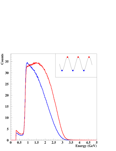
Figure 4: The energy spectrum of the detected positrons in red (blue) for a muon spin parallel (anti-parallel) to its momentum in the lab frame. The red line corresponds to the higher energy positrons. The inset shows the number of positrons as a function of time for an energy threshold of 2 GeV. The red dots correspond to the highest number of detected positrons above 2 GeV, whereas the blue to the lowest.

The angular frequency $\omega_{a}$ in the presence of both $E$ and $B$ fields is found [16, 17] to be

$$\vec{\omega}_{a}=-{e\over m_{\mu}}\left[a_{\mu}\vec{B}+\left({1\over\gamma^{2}-1}-a_{\mu}\right)\vec{\beta}\times\vec{E}\right],$$ (4)

where $\vec{\beta}\cdot\vec{E}=\vec{\beta}\cdot\vec{B}=0$ is assumed. The electric field influences $\omega_{a}$ because it advances the muon spin in its own rest frame (owing to Lorentz transformations, the electric field is partially transformed to a magnetic field) and the muon momentum in the lab frame. In the case of a realistic detector with finite energy and time resolution, there is some level of overlapping pulses (pileup), which produces a second harmonic of $\omega_{a}$ but also a first harmonic of $\omega_{a}$. More about the time development of these components and how we deal with them in our data is given later in the analysis section.

3.2 Magic Momentum

The muon anomalous magnetic moment has a value of approximately ${\alpha\over 2\pi}\approx{1\over 800}$, which is the second-order (dominant) QED contribution. Therefore, for $\gamma\approx 29.3$, the above equation (4) reduces to

$${\omega}_{a}=a_{\mu}{e\over m_{\mu}}{B}.$$ (5)

In Figure (5) we show the spin vector getting ahead of the momentum vector as a function of time.

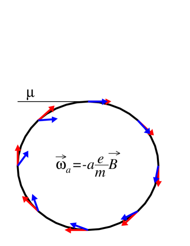
Figure 5: The muon spin $\vec{S}$ in its own rest frame gets ahead of its momentum vector $\vec{P}$ in the lab frame as time progresses. The detected energy spectrum of the electrons/positrons in the lab frame probes the product $\vec{S}\cdot\vec{P}$.

The reason equation (5) is valid comes from the fact that the g-2 precession is the difference between the muon spin precession in its own rest frame minus the momentum precession in the lab frame. The value of $\gamma\approx 29.3$ corresponds to the case where the radial $E$ field precesses the muon spin in its rest frame and momentum in the lab frame at the same rate. This is the reason for choosing a muon momentum of $P\approx 3.09\,{\rm GeV/}c$, a.k.a. “magic momentum” [19], which for $B=1.45$ T corresponds to a radius of $\approx 7.11$ m.

3.3 Origin of the Electric Field and Pitch Corrections

Due to finite muon beam momentum width the cancellation is not exact and there is a need for a small electric field correction. Also, the muon momentum may not be exactly orthogonal to the external magnetic field, so the Lorentz transformation of the lab electromagnetic fields into the rest frame fields are slightly modified. This effect introduces a small “pitch” correction. Both the $E$ field and pitch corrections are small, their sum being about +0.8 ppm.

3.4 Equation to Estimate $a_{\mu}$

A muon at rest and while in the presence of a magnetic field has its spin precessing with an angular frequency given by

$$\omega_{s}={g_{\mu}\over 2}\left({e\over m_{\mu}}\right)B.$$ (6)

When combined with equation (5), this yields

$$a_{\mu}={\omega_{a}\over\omega_{s}-\omega_{a}}={R\over\lambda-R}.$$ (7)

Here $R={\omega_{a}\over\omega_{p}}$, and $\omega_{p}$ is the angular frequency of the free proton in the $B$ field, measured with NMR techniques [20, 21]. One then also needs to know the ratio $\lambda={\omega_{s}\over\omega_{p}}$, the value of which is taken from another experiment. It follows that $\lambda={\mu_{\mu}\over\mu_{p}}$ with $\mu_{\mu}$ and $\mu_{p}$ the magnetic moments of muon and free proton respectively.

The precision with which $a_{\mu}$ can be evaluated is determined by the accuracy of $R$ and $\lambda$. The value of $\lambda$ is determined by measuring the microwave spectrum of the ground state of muonium [22], finding $\lambda=3.183\,345\,39(10)$. The precision of $R$ depends on the precision of $\omega_{a}$ and $\omega_{p}$. The quantity $\omega_{a}$ is estimated by detecting the electrons produced by the decay of the muons. The statistical uncertainty of $\omega_{a}$ is

$${\delta\omega_{a}\over\omega_{a}}={\sqrt{2}\over\omega_{a}\gamma\tau_{\mu}A\sqrt{N_{e}}}.$$ (8)

Here $A$ is the g-2 oscillation asymmetry and $N_{e}$ is the total number of detected positrons.

4 Beam Dynamics

4.1 Momentum Acceptance of the Muon g-2 Storage Ring

The injected muon beam debunches due to momentum dispersion with a lifetime of $\approx 25\,\rm\mu s$. The time spectrum of the positrons detected by a single detector at early times after injection is shown in Figure (6). The g-2 oscillation along with the slowly decaying fast rotation structure is clearly shown. The rotation frequency of the stored muons depends on their momentum. Therefore their momentum distribution can be found by Fourier analysis of the arrival times of the detected positrons. The momentum acceptance of the ring is narrow ($0.6\%$ total) and a special Fourier analysis technique is required to avoid introducing artificial effects into the width of the Fourier analyzed data [23]. The muon radial distribution so obtained is shown in Figure (7). The muon momentum distribution is inferred from the radial distribution using the formula $P_{\mu}=P_{0}\times[1+(R-R_{0})(1-n)/R_{0}]$, where $P_{0}$ is the central momentum, $R_{0}=7.112$ m is the center of the muon storage region, $R$ is the actual radial location of the muons, and $n$ is the field focusing index.

The fast-rotation structure is eliminated by randomizing the time of the injected muon beam with the average fast rotation period of approximately 149.2 ns, the result shown in Figure (8). After the randomization the Fourier analysis spectrum shows no structure at the fast rotation frequency.

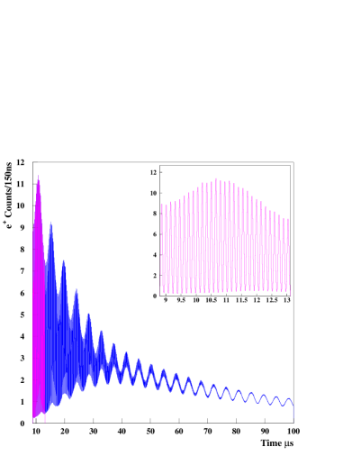
Figure 6: The bunched structure of the muon beam, clearly evident in the inset showing the $8.5-13\,\rm\mu s$ time range, distorts the g-2 oscillation at early times. The fast structure is decaying with a lifetime of $\approx 25\,\rm\mu s$ with only the g-2 oscillation remaining at later times.

Figure 7: The muon radial distribution obtained by Fourier analyzing the fast rotation structure of Figure (6). The central vertical line corresponds to the center of the muon storage region with $R_{0}=7.112$ m and the two lines on either side are the edges of the storage region at $R_{0}\pm 4.5$ cm.

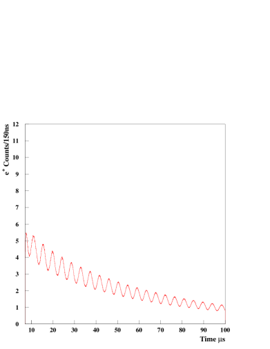
Figure 8: The detected positron time spectrum of Figure (6) after randomizing the muon injection time with a period of 149.2 ns; the fast rotation structure seen before, is eliminated.

4.2 Coherent Betatron Oscillation Frequencies

The muon storage ring lattice is shown in Figure (9). The muon beam is injected through the inflector [24] whose acceptance is smaller than that of the ring itself. This fact has as a result that the phase space of the betatron oscillations is not filled, resulting in betatron oscillations of the beam as a whole, called coherent betatron oscillations (CBO). Those oscillations are both horizontal and vertical and their amplitudes are described by:

$$x=x_{e}+x_{0}\cos{(\omega_{x}t+\theta_{x})},$$ (9)

$$y=y_{0}\cos{(\omega_{y}t+\theta_{y})},$$ (10)

where $x_{e}$ is the horizontal equilibrium radial position away from the $R_{0}=7.112$ m center of the ring, and $x_{0}$ ($y_{0}$) is the horizontal (vertical) CBO amplitude. The $\omega_{x}\equiv 2\pi f_{x}$, $\omega_{y}\equiv 2\pi f_{y}$, with $f_{x}$ ($f_{y}$) the horizontal (vertical) CBO frequencies given by

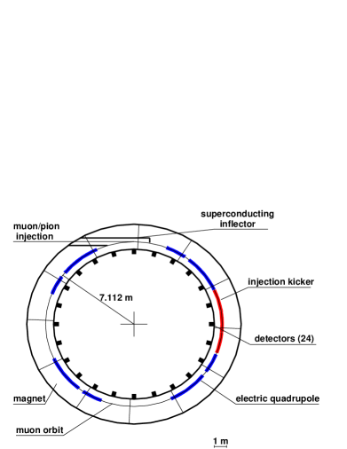
Figure 9: The muon g-2 ring lattice indicating the four quadrupole regions, the kicker region and the inflector location. The muon storage region is a torus of radius $R_{0}=7112$ mm and a cross section of a circle with a diameter of 90 mm. The inner ring of 24 detectors is shown as black squares.

$$f_{x}\simeq f_{c}(1-\sqrt{1-n}),$$ (11)

and

$$f_{y}\simeq f_{c}\sqrt{n},$$ (12)

where $f_{c}={1\over 149.2{\rm ns}}=6.7$ MHz, the cyclotron frequency, and $n$ is the field focusing index. Equations (11,12) are not exact due to the discrete nature of the quadrupole coverage of the ring. There are small corrections given in reference [15].

4.3 Field Focusing Index for the 2000 Run

In Figure (10) we show the vertical $\nu_{y}\simeq\sqrt{n}$ versus the horizontal $\nu_{x}\simeq\sqrt{1-n}$ tune, along with the most important beam dynamics resonances of our weak focusing muon storage ring. The acceptance of a weak focusing ring has a rather wide maximum at $n=0.5$, being at $90\%$ of its maximum at $n=0.137$.

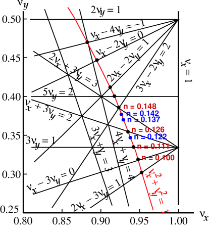
Figure 10: The tune plane with the most important beam dynamics resonances of our weak focusing muon storage ring. The 2000 run was mostly taken at $n\simeq 0.137$, in the middle of two relatively strong resonances, at $n=0.126$ and $n=0.148$. The 2001 run was taken at $n=0.142$ and $n=0.122$.

The $n$ value is proportional to the voltage applied to the quadrupole plates, Figure (11). Due to the presence of the magnetic field, and for reasonable residual pressures in the vacuum chamber of about $10^{-7}$ Torr, it would be very difficult to work at $n=0.5$. This is so because there is a large number of low-energy trapped electrons circulating in the quad region [15]. A reasonable number to work with was around $n=0.136-0.137$, in the middle between two relatively strong beam dynamics resonances at $n=0.126$, and $n=0.148$, shown in Figure (10). The effect of the low-energy trapped electrons has been studied and is shown to contribute less than 0.01 ppm to the magnetic field. Their effect on the quadrupole electric field is negligible [15].

From equation (11) we have that the horizontal frequency corresponds to $f_{x}\simeq 466$ kHz which is very near twice the g-2 frequency of $\approx 229.1$ kHz.

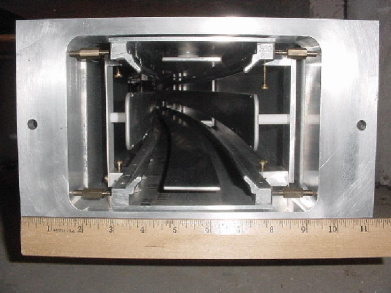
Figure 11: A photograph of the electrostatic quadrupoles taken from the end of a vacuum chamber; the ring center is on the left. The ruler units are in inches.

5 Analysis of $\omega_{a}$

In the year 2000, we had a very successful run in terms of accumulating a lot of statistics. In Figure (12) we show the total number of positrons detected with $E>2$ GeV as a function of time. The equation describing the ideal positron time spectrum is given by

$$N(t)=N_{0}(E)\,e^{-\gamma\tau_{\mu}}\,[1+A(E)\,\cos{(\omega_{a}t+\phi_{a}(E))}],$$ (13)

where $A(E)$ corresponds to the g-2 oscillation asymmetry and $\phi_{a}(E)$ the g-2 phase, both of which depend on the energy threshold $E$; for $E=2$ GeV, $A=0.4$.

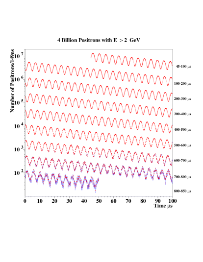
Figure 12: The number of positrons detected with $E>2$ GeV as a function of time. The error bars are shown in blue and the points in red.

The Fourier analysis of the residuals of the fits to the data using equation (13) is shown in Figure (13). The amplitude of the various peaks, especially that of $f_{\rm CBO}\equiv f_{x}$ has a large amplitude relative to the white noise present in the spectrum, implying that the CBO modulation is statistically very important. The two CBO sidebands are not of equal amplitude and in particular not equal to ${1\over 2}AA_{\rm N}$, with $A_{\rm N}$ the amplitude at $f_{x}$. This precludes that $N_{0}$ is the only CBO modulated parameter as was assumed in the 1999 data analysis [25].

Figure 13: Fourier analysis of the residuals to the fits to the data of Figure (13) using equation (13). $f_{\rm CBO}\equiv f_{x}$ has a large amplitude implying that the CBO modulation is important.

At early times the number of positrons shown in Figure (12) is of order 10 million per 149.2 ns bin. Therefore, very small beam dynamics effects are important and noticeable in the least $\chi^{2}$ fits. Since the acceptance of the detectors depends on the position of the muon beam relative to the detectors, the time and energy spectra of the detected positrons are modulated with the CBO frequency. As a result, the g-2 phase, asymmetry and the normalization $N_{0}$ are all modulated with the CBO frequency, thus becoming all time dependent. Since the CBO frequency is very close to twice the g-2 frequency, it turns out [6] that the asymmetry and g-2 phase modulation are important effects that need special attention, consistent with M.C. simulations. The way they manifest themselves is by phase pulling the g-2 frequency with an oscillation period of $T_{o}={1\over(f_{x}-f_{a})-f_{a}}\approx 130\,\rm\mu s$. The CBO modulation affects, as we said earlier, the energy spectrum of the detected positrons and hence their average energy as a function of time. However, since the oscillation period is $\approx 130\,\rm\mu s$, it was difficult to distinguish it from other slow effects like gain change, muon losses, and pileup. In 2001, we took data at different $n$ values, specifically at $n=0.142$ and $n=0.122$ corresponding to a horizontal CBO frequency of 491 kHz and 421 kHz, respectively.

The time dependence of the CBO modulated effects is given by:

1. $N_{0}(t)=N_{0}\,[1+A_{N}\,e^{-t/\tau_{x}}\,\cos{(2\pi f_{x}t+\phi_{N})}]$, with $\tau_{x}$ the lifetime of the CBO modulation found from the data to be of the order of $\approx 100\rm\,\mu s$.

2. $A(t)=A_{0}\,[1+A_{A}\,e^{-t/\tau_{x}}\,\cos{(2\pi f_{x}t+\phi_{A})}]$,

3. $\phi_{a}(t)=\phi_{a0}+A_{\phi}\,e^{-t/\tau_{x}}\,\cos{(2\pi f_{x}t+\phi_{\phi})}$

The time dependence of $N_{0}(t)$ was found by strobing the energy spectrum of the 2001 data at the g-2 frequency, see Figures (14,15). The fitting function used was of the form: $P_{1}\,\sin{(2\pi t/P_{2}+P_{3})}\,e^{-t/P_{4}}$. Next it was verified by looking at the residuals after the 5-parameter fit to the data, minimizing $\chi^{2}$ by fitting the data with various functions, M.C. simulations, etc. The time dependence used for $A(t)$ and $\phi(t)$ was not possible to verify from the data, only the M.C. simulations showed that they could not be too far off.

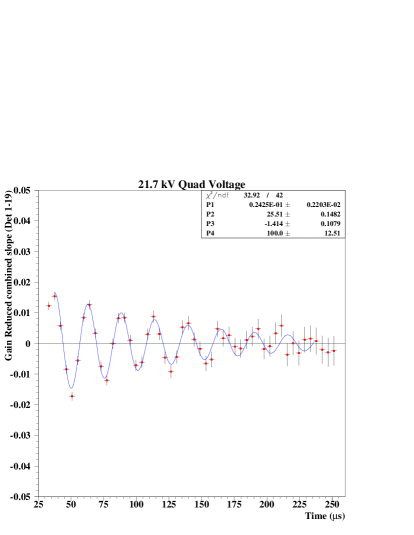
Figure 14: By strobing the energy spectrum of the detected electrons of the 2001 data we were able to observe the time dependence of $N_{0}(t)$. The high voltage was 21.7 kV, and $n=0.122$.

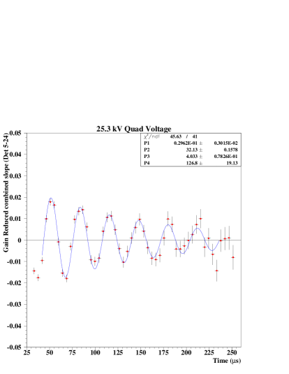
Figure 15: Same as in Figure (14) but for the case where the high voltage was 25.3 kV, and $n=0.142$.

The amplitudes of $A_{N}$, $A_{A}$, and $A_{\phi}$ are consistent with values from M.C. simulations. The values of the phases $\phi_{N}$ versus detector from the fits to the data are consistent with running from 0 to $2\pi$. That means that if the sum of all detectors is used, the amplitudes of $A_{N}$, $A_{A}$, and $A_{\phi}$ are reduced substantially, consistent with the values obtained with fits to the sum.

The phase pulling of g-2 due to CBO is best depicted in Figure (16) where a straight line fit to $f_{a}\equiv\omega_{a}/2\pi$ versus detector gives $f_{a}=229\,073.98\pm 0.14$ Hz and a $\chi^{2}=58.7/21$, indicating that there is a consistency problem. A fit to a sine wave plus a constant, $f_{a}+P_{1}*\sin{({2\pi\over 24}\times det.\#+P_{2})}$, to the same data gives $f_{a}=229\,074.02\pm 0.14$ Hz and a $\chi^{2}=24.3/19$ with $P_{1}=(1.20\pm 0.20)$ Hz, and $P_{2}=1.91\pm 0.17$ rad.

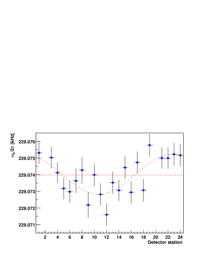
Figure 16: A straight line fit to $\omega_{a}/2\pi$ versus detector number when only the ideal 5 parameter function is used to fit the positron time spectrum. The $\chi^{2}$ for the straight line fit is $\chi^{2}=58.7/21$, and the average $f_{a}=229\,073.98\pm 0.14$ Hz. A sine wave fit (see text) gives a good $\chi^{2}$ and a central $f_{a}=229\,074.02\pm 0.14$ Hz, very close to the average.

When the CBO modulation is included for the parameters $N_{0}(t)$, $A(t)$, and $\phi_{a}(t)$, the $\chi^{2}$ to a straight line fit of $f_{a}$ versus detector, Figure (17), is $\chi^{2}=23.9/21$, and the average $f_{a}=229\,073.92\pm 0.14$ Hz.

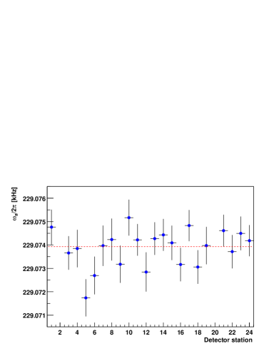
Figure 17: A straight line fit to $\omega_{a}/2\pi$ versus detector number when the ideal 5 parameter function including the CBO modulations of $N_{0}(t)$, $A(t)$, and $\phi(t)$, is used to fit the positron time spectrum. The $\chi^{2}$ for the straight line fit is $\chi^{2}=23.9/21$, and the average $f_{a}=229\,073.92\pm 0.14$ Hz.

5.1 Different Approaches to the CBO Modulation and Slowly Varying Effects

We have used several different approaches to analyze the data taken in 2000:

• Positrons with $E>2$ GeV and a function including the modulation of $N_{0}(t)$ and $A(t)$ with $f_{x}$.

• Positrons in 200 MeV energy bins with $1.4<E<3.2$ GeV and a function including the modulation of $N_{0}(t)$, $A(t)$, and $\phi(t)$ with $f_{x}$.

• Ratio method [25]; $\omega_{a}$ becomes independent of slow effects, e.g. muon losses.

All the above methods gave results that are consistent among themselves within the expected statistical uncertainties due to the slightly different data used.

In a side study, using positrons with $E>2$ GeV, we strobed the data at the horizontal CBO frequency $f_{x}$ making $\omega_{a}$ independent of the CBO parameters. Since $f_{x}$ is slightly higher than twice the g-2 frequency, one can recover all the information regarding the g-2 frequency, satisfying the Nyquist limit. Therefore the frequency, amplitude, and phase are recovered using mainly only the 5-parameter function and thus making no assumption as to the CBO functional form whatsoever. This method gave, again, consistent results with the above methods.

5.2 Pileup and other Systematic Errors

When a positron arrives at the electromagnetic calorimeter and deposits an energy greater than approximately 1 GeV, it triggers the WFD connected to that particular detector. The WFDs are always running, and they were designed to keep in their memory more data, before and after the pulse, than is necessary to reconstruct the positron signal that triggered them. This fact turned out to be of great help in dealing with the pileup pulses. Due to high rates in 2000, the overlapping of two positron pulses constitutes approximately $0.5\%$ of all detected pulses. We used the extra recorded data to reconstruct, on a statistical basis, the time and energy spectrum of the pileup pulses which we then subtract from the data; see Figure (18) [25].

Figure 18: The energy spectrum of the detected positrons with energy greater that 1 GeV at all times (thick line) and at only late times (thin line) when the rates are low. The dashed line shows the pileup-subtracted spectrum at all times. The inset shows the average energy of positrons before (filled circles) and after (open circles) pileup subtraction for $E>2$ GeV.

The total systematic uncertainty in $\omega_{a}$ is 0.31 ppm [6]. The final $f_{a}=229\,074.11(14)(7)$ Hz (0.7 ppm) which includes a total correction of +0.76(3) ppm due to electric field [16] and pitch [16, 26] corrections. Those corrections have been studied in many different ways: analytically, particle tracking and spin tracking. For the latter, the BMT [27] equations were applied with our ring parameters, following the equations of chapter 11.11 (pages 556-560) of reference [17]. The results from all the above methods are in agreement to $\approx 0.01$ ppm.

6 Analysis of $\omega_{p}$

The magnetic field of the muon storage region was measured with an NMR trolley every two to three days while in between it was followed by 367 fixed NMR probes located on top and bottom of the vacuum chambers. The average B-field, convoluted over the muon distribution, was obtained by two largely independent analyses of $\omega_{p}$ [6]. The magnetic field multipoles integrated over the azimuth of the ring for one trolley run out of 22 are shown in Figure (19); the central field was $1.451\,274$ T. The final $\omega_{p}/(2\pi)=61\,791\,595(15)$ Hz. The total systematic uncertainty in $\omega_{p}$ is 0.24 ppm [6].

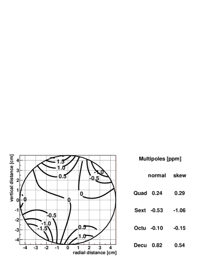
Figure 19: The magnetic field multipoles integrated over the azimuth of the ring for one trolley run.

7 Results

In order to compute $a_{\mu}$, both $\omega_{a}$ and $\omega_{p}$ values are necessary. The analysis groups dealing with $\omega_{a}$ and $\omega_{p}$ worked separately and had applied secret offsets to their results until it was decided the analyses were finished. This avoided biases that could influence the choice of data selection, analysis method, etc. After the analyses seemed complete, during a collaboration meeting a secret ballot was held of whether or not we should reveal the offsets and compute $a_{\mu}$. It was unanimous for revealing the offsets and compute $a_{\mu}$, which we did. The results are

$$a_{\mu^{+}}={R\over\lambda-R}=11\,659\,204(7)(5)\times 10^{-10},$$ (14)

with a relative error of 0.7 ppm. The experimental world average becomes

$$a_{\mu}(exp)=11\,659\,203(8)\times 10^{-10},$$ (15)

with again a relative error of 0.7 ppm. This experiment, like most of the muon experiments, is still statistics limited.

In Figure (20) we give the recent BNL $a_{\mu}(exp)$ values, the average and the theoretical values based on the current standard model with the $e^{+}e^{-}$ data (solid horizontal line) and the $\tau$ data (dashed line) for the hadronic contribution [9].

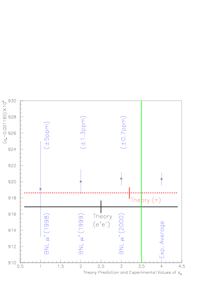
Figure 20: The experimental values of $a_{\mu}$ compared to the theoretical $a_{\mu}$ based on the current standard model with the $e^{+}e^{-}$ data (solid horizontal line) and the $\tau$ data (dashed line) for the hadronic contribution [9].

8 Discussion and Future Prospects

The difference between the experimental value and the current theoretical prediction of $a_{\mu}$ is

$$a_{\mu}({\rm exp})-a_{\mu}({\rm SM})=34(11)\times 10^{-10}$$ (16)

which is a little over three standard deviations and it may indicate new physics. One should, however, wait for confirmation of the $e^{+}e^{-}$ data and understand the reason why the $\tau$ based data imply a higher hadronic contribution than the $e^{+}e^{-}$ data, before making any claims as to whether or not new physics has been seen. The difference $a_{\mu}({\rm exp})-a_{\mu}({\rm SM})=17(11)\times 10^{-10}$, i.e. only 1.5 sigma, when the $\tau$ data are used. On the experimental side, we have already accumulated about 3 billion electrons with $E>2$ GeV, equivalent to a statistical power of approximately 0.7 ppm, from our 2001 run with negative muons. We are currently analyzing those data and expect to finish by early next year. We also have scientific approval for an extra four month period which the High Energy Division of DOE has not yet approved, though they should, in order to properly conclude the experiment.

Assuming that the $e^{+}e^{-}$ data will hold, and if supersymmetry is responsible for the g-2 deviation, an EDM from similar quantum loops but with a phase giving rise to T and P violation is natural and likely. That would make the muon one of the best places to search for an EDM [28]. Such an effort is currently underway [29]. It promises to be sensitive to physics beyond the standard model [30, 31, 32, 33, 34] and to continue the exciting muon physics of the past and present.

References

- [1] Proceedings of my plenary talk at ICHEP02, Amsterdam, 31 July 2002.
-
[2]
G.W. Bennett2, B. Bousquet9,
H.N. Brown2, G. Bunce2,
R.M. Carey1, P. Cushman9, G.T. Danby2, P.T. Debevec7,
M. Deile11, H. Deng11, W. Deninger7, S.K. Dhawan11,
V.P. Druzhinin3, L. Duong9, E. Efstathiadis1, F.J.M. Farley11,
G.V. Fedotovich3, S. Giron9, F.E. Gray7, D. Grigoriev3,
M. Grosse-Perdekamp11, A. Grossmann6, M.F. Hare1, D.W. Hertzog7,
X. Huang1, V.W. Hughes11, M. Iwasaki10, K. Jungmann5,
D. Kawall11, B.I. Khazin3, J. Kindem9, F. Krienen1,
I. Kronkvist9, A. Lam1, R. Larsen2, Y.Y. Lee2,
I. Logashenko1,3, R. McNabb9, W. Meng2, J. Mi2, J.P. Miller1,
W. Morse2, D. Nikas2, C.J.G. Onderwater7, Y. Orlov4,
C.S. zben2, J.M. Paley1, Q. Peng1, C.C. Polly7, J. Pretz11,
R. Prigl2, G. zu Putlitz6, T. Qian9, S.I. Redin3,11, O. Rind1,
B.L. Roberts1, N. Ryskulov3, P. Shagin9, Y.K. Semertzidis2,
Yu.M. Shatunov3, E.P. Sichtermann11, E. Solodov3, M. Sossong7,
A. Steinmetz11, L.R. Sulak1, A. Trofimov1, D. Urner7,
P. von Walter6, D. Warburton2, and A. Yamamoto8.
1Boston University, 2Brookhaven National Laboratory, 3Budker Institute of Nuclear Physics, 4Cornell University, 5Kernfysisch Versneller Instituut, 6Physikalisches Institute der Universitat Heidelberg, 7University of Illinois, 8KEK, 9University of Minnesota, 10Tokyo Institute of Technology, 11Yale University. - [3] M. Davier and A. Hcker, Phys. Lett. B435, 427 (1998).
- [4] J. Hisano, hep-ph/0204100(2002).
- [5] Z. Bern, plenary session talk at ICHEP02 and these proceedings.
- [6] G.W. Bennett et al., Phys. Rev. Lett. 89, 101804 (2002).
- [7] E. de Rafael, hep-ph/0208251.
- [8] T. Teubner, Parallel session talk at ICHEP02 and these proceedings.
- [9] M. Davier et al., hep-ph/0208177.
- [10] A. Czarnecki and W.J. Marciano, Phys. Rev. D64, 013014 (2001).
- [11] B. Krause, Phys. Lett. B390,392 (1997); R. Alemany, M. Davier, and A. Hcker, Eur. Phys. J. C2, 123 (1998).
- [12] M. Knecht et al., Phys. Rev. Lett. 88, 071802 (2002); M. Knecht and A. Nyffeler, Phys. Rev. D65, 073034 (2002); M. Hayakawa and T. Kinoshita, hep-ph/0112102; J. Bijnens, E. Pallante, and J. Prades, Nucl. Phys. B626, 410 (2002); I. Blokland, A. Czarnecki, and K. Melnikov, Phys. Rev. Lett. 88, 071803 (2002).
- [13] P. Mohr and B. Taylor, Rev. Mod. Phys. 72, 351 (2000).
- [14] E. Efstathiadis et al., accepted for publication in Nucl. Instrum. Meth. A.
- [15] Y.K. Semertzidis et al., accepted for publication in Nucl. Instrum. Meth. A.
- [16] F.J.M. Farley and E. Picasso, in Quantum Electrodynamics, edited by T. Kinoshita (World Scientific, Singapore, 1990).
- [17] J.D. Jackson, Classical Electrodynamics, John Wiley and Sons, NY, 1975.
- [18] S. Sedykh et al., Nucl. Instrum. Meth. A455, 346 (2000).
- [19] J. Baily et al., Nucl. Phys. B150, 1 (1979).
- [20] R. Prigl et al., Nucl. Instrum. Meth. A374, 118 (1996).
- [21] X. Fei, V. Hughes, and R. Prigl, Nucl. Instrum. Meth. A394, 349 (1997).
- [22] W. Liu et al., Phys. Rev. Lett. 82, 711 (1999).
- [23] Y. Orlov, C.S. zben, and Y.K. Semertzidis, Nucl. Instrum. Meth. A482, 767 (2002).
- [24] A. Yamamoto et al., accepted for publication in Nucl. Instrum. Meth. A.
- [25] H.N. Brown et al., Phys. Rev. Lett. 86, 2227 (2001).
- [26] F.J.M. Farley, Phys. Lett. B42, 66 (1972).
- [27] V. Bargmann, L. Michel, and V.L. Telegdi, Phys. Rev. Lett. 2, 435 (1959).
- [28] W.J. Marciano, private communication.
- [29] Y.K. Semertzidis et al., [hep-ph/0012087] and Letter of Intent to BNL, “Sensitive Search for a Permanent Muon Electric Dipole Moment”, for more info see http://www.bnl.gov/edm/.
- [30] A. Pilaftsis, Nucl. Phys. B644, 263 (2002).
- [31] K.S. Babu, B. Dutta, and R.N. Mohapatra, Phys. Rev. Lett. 85, 5064 (2000).
- [32] J.L. Feng, K.T. Matchev, and Yael Shadmi, Nucl. Phys. B613, 366 (2001).
- [33] J.R. Ellis et al., Phys. Lett. B528 86 (2002).
- [34] A. Romanino and A. Strumia, Nucl. Phys. B622, 73 (2002).