Landau-Pomeranchuk-Migdal resummation for dilepton production

Abstract

We consider the thermal emission rate of dileptons from a QCD plasma in the small invariant mass ($Q^{2}\sim g_{\rm s}^{2}T^{2}$) but large energy ($q^{0}\mbox{~{}{\raisebox{1.72218pt}{$>$}} {\raisebox{-2.58334pt}{$\sim$}}~{}}T$) range. We derive an integral equation which resums multiple scatterings to include the LPM effect; it is valid at leading order in the coupling. Then we recast it as a differential equation and show a simple algorithm for its solution. We present results for dilepton rates at phenomenologically interesting energies and invariant masses.

1. Laboratoire d’Annecy-le-Vieux de Physique Théorique, B.P. 110,
   UMR 5108 du CNRS associée à l’Université de Savoie,
   74941 Annecy-le-Vieux Cedex, France

2. Service de Physique Théorique, Bat. 774, CEA/Saclay,
   91191, Gif-sur-Yvette Cedex, France

3. Department of Physics, University of Washington,
   Seattle, Washington 98195, USA
   and
   Department of Physics, McGill University,
   3600 rue University, Montréal QC H3A 2T8, Canada

4. Physics Department, University of Winnipeg,
   Winnipeg, Manitoba R3B 2E9, Canada

SPhT-T02/150, LAPTH-946/02

1 Introduction

In the last few years progress has been achieved in understanding the production of electromagnetic probes in a quark-gluon plasma in equilibrium. In the case of a hard photon (which is defined as having an energy larger than the temperature T of the plasma) the usual Compton and annihilation processes discussed long ago [1, 2] are not the only leading-order mechanisms. It turns out that bremsstrahlung of a quark in a plasma gives a leading contribution [3, 4] and, more importantly, a crossed process from bremsstrahlung actually dominates at a large enough energy [5, 6, 7, 8]. This process, sometimes referred to as off-shell annihilation or annihilation with scattering, is of type 3-$body\rightarrow$ 2-$body$ : the photon is produced via quark-antiquark annihilation where one of the incoming quarks is put off-shell by scattering in the plasma. However, the formation time of the photon is comparable to, or larger than, the average time between soft scatterings of a quark in the plasma (inverse of the damping rate). This implies that multiple scattering plays an important role in these photon emission processes [9].

A correct treatment of multiple scattering, even after performing Hard Thermal Loop (HTL) resummation [10], involves the resummation of ladder diagrams with effective propagators for both fermions and gluons. This resummation leads to an integral equation, which has been solved to give the photon emission rate to leading order in the strong coupling $g_{\rm s}$ [11, 12, 13]. The resummation of higher loop diagrams implements the Landau-Pomeranchuk-Migdal [14, 15, 16] effect which has been much discussed recently in the context of jet energy loss in a hot medium [17, 18, 19, 20, 21, 22, 23]. However, there are differences between the approach followed here for photon production and that used for jet quenching: we work consistently in the HTL approach, using the actual distribution of moving charges in the plasma and dynamical screening of interactions, rather than a model of static, Debye screened charges. Note that no magnetic mass needs to be introduced in order to screen transverse gluons, since ultrasoft divergences have been shown to cancel thanks to cancellations between diagrams of different topologies [11] (see also [24, 25, 26, 27]).

Preliminary hydrodynamical studies [28, 29, 30, 31, 32], which take into account the above mechanisms of photon production, show that the thermal rate (including the contribution from the hot hadronic phase) should clearly emerge above prompt photon sources (produced in the early stages of the collisions) in a range from 1 GeV $-$ 3 GeV to 5 GeV at RHIC and LHC.

The above developments are quite timely in view of the recent WA98 measurements at SPS [33] and of the upcoming results at RHIC where the photon spectrum in gold-gold collisions is being measured [34]. There is however an uncertainty concerning the possibility of separating the spectrum of direct photons from that of photons which are decay products of resonances, in particular $\pi^{0}$’s. In the energy range of interest the $\pi^{0}$ signal may be almost two orders of magnitude above the direct photon rate and the subtraction of the $\pi^{0},\ \eta,\ \cdots$ background from the data is a formidable experimental challenge.

In the mean time it is interesting to consider an alternative channel which carries the same dynamical information as the real photon production rate, but which suffers a different, less important, background. This is the case of the production of low mass lepton pairs at large momentum. The invariant mass of the pair should be high enough to be above the background of Dalitz pairs from the pions, but small enough that the rate remains appreciable. Typically one expects the range 150 Mev $<\sqrt{Q^{2}}<$ 500 MeV to be realistic for our purposes ($\sqrt{Q^{2}}$ is the invariant mass of the lepton pair). Higher mass ranges (above the vector meson masses) should also be explored.

This rate has already been calculated for the Drell-Yan process [35], for the $2\to 2$ processes [36, 37], and for bremsstrahlung and off-shell annihilation in the approximation where the quark undergoes a single scattering in the medium [38]. The analysis of multiple scattering is clearly called for. Compared to the real photon case, the results of [38] show increased technical difficulties associated with the much more complicated analytic structure of the diagrams: more unitarity cuts contribute and the cancellation of divergences between the various cuts is a subtle affair. In accordance with general theorems of perturbation theory [39], the calculated rate turns out to be finite everywhere except at the $q\bar{q}$ threshold ($Q^{2}=4M_{\infty}^{2}$, $M_{\infty}$ the quark thermal mass) where there remain integrable (square root and logarithm) singularities. However, this threshold is right where the formation time is the longest, and rescattering effects are expected to be largest. Therefore the two loop analysis [38] is not reliable here.

The object of this paper is to compute the imaginary part of the retarded current-current correlator, at momentum $Q$ which is hard ($q^{0}\mbox{~{}{\raisebox{1.72218pt}{$>$}} {\raisebox{-2.58334pt}{$\sim$}}~{}}T$) but near the light cone ($Q^{2}\sim g_{\rm s}^{2}T^{2}$), at leading order in $g_{\rm s}$. This current-current correlator is related to the dilepton production rate, per lepton species, via [40]

$$\frac{dN_{{}_{\ell^{+}\ell^{-}}}}{d^{4}xd^{4}Q}=\frac{\alpha_{{}_{\rm EM}}}{12\pi^{4}Q^{2}(e^{q^{0}/T}-1)}\,{\rm Im}\>\Pi_{{}_{R}}{}^{\mu}_{\mu}(Q)\,.$$ (1)

The calculation requires a resummation of diagrams analogous to that for real photon production. We first review the integral equation already obtained [11] in the case of a real photon ($Q^{2}=0$). Then we extend it to off shell photons. Besides minor kinematic changes to the treatment of [11], this also requires inclusion of longitudinally polarized virtual photons. It is then shown how to obtain an ordinary differential equation by going to impact parameter space, where the equation is solved numerically. The result is more complete, and in some ways simpler, than the two loop perturbative one. We find that multiple scattering effects completely remove the $q\bar{q}$ threshold behavior found in the perturbative treatment; the dilepton spectrum is nonsingular and smooth. Finally, we discuss some phenomenological applications.

2 LPM corrections for longitudinal photons

In this section, we leave aside the production of photons by Compton scattering ($gq\rightarrow\gamma q$) and annihilation ($q\bar{q}\rightarrow\gamma g$) which appear at one loop in the perturbative expansion of the HTL effective theory [36, 37] and we consider only the processes of type $qi\rightarrow\gamma qi$ and $q\bar{q}i\rightarrow\gamma i$ where $i$ denotes a quark, an antiquark or a gluon. These appear at the two-loop level but because of a strong collinear enhancement, powers of $T^{2}/M_{\infty}^{2}\sim 1/g_{\rm s}^{2}$ are generated so that they contribute at the leading order in the strong coupling. Higher order diagrams with a ladder topology involve the same enhancement mechanism [each new rung in the ladder brings a factor of ${\cal O}(g_{\rm s}^{2}/g_{\rm s}^{2})$] and therefore they also contribute at leading order. The summation of these dominant diagrams leads to an integral equation which we now discuss [11, 12, 13].

2.1 Reminder: transverse modes

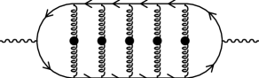
Figure 1: Typical diagram which must be resummed to determine $\,{\rm Im}\>\Pi_{\mu}^{\mu}$. The gluon lines are soft and HTL-resummed, the solid (quark) lines are hard, approximately on-shell, and resummed to include the dominant imaginary part.

In [11, 12, 13], Arnold, Moore, and Yaffe summed the set of diagrams of the form shown in Fig. 1, for lightlike external momentum $Q$. The lightlike condition allowed them to consider only the two transverse polarizations; in general $\Pi^{\mu\nu}$ has contributions from three polarizations (not four, because $Q_{\mu}\Pi^{\mu\nu}=0$), but when $Q^{2}=0$ the longitudinal polarization also vanishes. In terms of the retarded photon polarization tensor, we can rewrite the result presented in these papers as follows:

$$\sum_{i=1,2}{\rm Im}\,\Pi_{{}_{\rm R}}{}_{i}^{i}(Q) \approx {{e^{2}N_{\rm c}}\over{8\pi}}\int_{-\infty}^{+\infty}dp_{0}\,\;[n_{{}_{F}}(r_{0})-n_{{}_{F}}(p_{0})]\;{{p_{0}^{2}+r_{0}^{2}}\over{(p_{0}r_{0})^{2}}}$$ (2)

$$\qquad\;\;\qquad\times\,{\rm Re}\>\int{{d^{2}{\boldsymbol{p}}_{\perp}}\over{(2\pi)^{2}}}\;2{\boldsymbol{p}}_{\perp}\cdot{\boldsymbol{f}}({\boldsymbol{p}}_{\perp})\;,$$

with $r_{0}\equiv p_{0}+q_{0}$, $n_{{}_{F}}(p_{0})\equiv 1/(\exp(p_{0}/T)+1)$ the Fermi-Dirac statistical weight, and where the dimensionless function ${\boldsymbol{f}}({\boldsymbol{p}}_{\perp})$ obeys the following integral equation:

$$2{\boldsymbol{p}}_{\perp}=i\delta E{\boldsymbol{f}}({\boldsymbol{p}}_{\perp})+g_{\rm s}^{2}C_{{}_{\rm F\hskip 0.50003pt}}T\!\!\int{{d^{2}{\boldsymbol{l}}_{\perp}}\over{(2\pi)^{2}}}\,{\cal C}({\boldsymbol{l}}_{\perp})\,[{\boldsymbol{f}}({\boldsymbol{p}}_{\perp})-{\boldsymbol{f}}({\boldsymbol{p}}_{\perp}+{\boldsymbol{l}}_{\perp})]\;.$$ (3)

In this integral equation, $\delta E\equiv q_{0}({\boldsymbol{p}}_{\perp}^{2}+M_{\infty}^{2})/(2p_{0}r_{0})$ is an energy denominator arising from nearly on-shell quark propagators; it can be interpreted as the inverse formation time of the photon. Here $M_{\infty}^{2}\equiv g_{\rm s}^{2}C_{{}_{\rm F\hskip 0.50003pt}}T^{2}/4$ is the thermal mass of a hard quark at leading order (or equivalently, in the HTL approximation). $C_{{}_{\rm F\hskip 0.50003pt}}=(N_{\rm c}^{2}-1)/2N_{\rm c}$ is the Casimir in the fundamental representation of the gauge group $SU(N_{\rm c})$; in QCD it is 4/3. The second term arises from the gluon exchange lines in Fig. 1 (both those shown and those hidden in the fact that the quark line self-energies are resummed). The factor ${\cal C}({\boldsymbol{l}}_{\perp})$ is the kernel of a collision integral describing an elementary collision of the emitter with another particle of the plasma. In terms of the transverse and longitudinal HTL self-energies $\Pi_{{}_{T,L}}(l_{0}/l)$ of the exchanged gluon, it is given by [11, 12, 13]:

$${\cal C}({\boldsymbol{l}}_{\perp}) \!\!\equiv\!\! \int{{dl_{0}dl_{z}}\over{(2\pi)^{2}}}2\pi\delta(l_{0}-l_{z})\,{1\over{l_{0}}}$$ (4)

$$\hskip 23.99997pt\times\sum_{\alpha=L,T}{{2{\rm Im}\,\Pi_{\alpha}(L)}\over{(L^{2}-{\rm Re}\,\Pi_{\alpha}(L))^{2}+({\rm Im}\,\Pi_{\alpha}(L))^{2}}}\;P_{\alpha}^{\mu\nu}(L)\widehat{Q}_{\mu}\widehat{Q}_{\nu}\;,$$

with $\widehat{Q}_{\mu}\equiv(1,{\boldsymbol{q}}/q)$ and $P_{{}_{T,L}}^{\mu\nu}(L)$ the transverse or longitudinal projector for a gluon of momentum $L$. In [8], it was shown that this collision kernel can in fact be calculated exactly thanks to a sum rule satisfied by the HTL gluon propagator, leading to a very simple expression:

$${\cal C}({\boldsymbol{l}}_{\perp})={1\over{{\boldsymbol{l}}_{\perp}^{2}}}-{1\over{{\boldsymbol{l}}_{\perp}^{2}+m_{{}_{\rm D}}^{2}}}\;,$$ (5)

where $m_{{}_{\rm D}}^{2}\equiv g_{\rm s}^{2}T^{2}[N_{\rm c}+N_{{}_{\rm F}}/2]/3$ is the Debye mass in an $SU(N_{\rm c})$ gauge theory with $N_{{}_{\rm F}}$ fundamental representation flavors.

Generalizing the above equations to the case of the transverse modes of a massive photon is straightforward, as one needs only to replace $M_{\infty}^{2}$ in $\delta E$ by the following combination of the quark mass and the photon invariant mass [4, 12] :

$$M_{\infty}^{2}\to M_{\rm eff}^{2}\equiv M_{\infty}^{2}+{{Q^{2}}\over{q_{0}^{2}}}p_{0}r_{0}\;.$$ (7)

For $Q^{2}>4M_{\infty}^{2}$, this quantity can become negative and $\delta E$ can vanish. In this case, $M_{\rm eff}^{2}$ should be understood as having an infinitesimal imaginary part $ip_{0}r_{0}\epsilon/q_{0}$, as one can readily see from its derivation from the quark energy denominators.

This is not enough to fully calculate the dilepton production rate; one must also include the longitudinal mode of the off shell (virtual) photon. We calculate the contribution of this mode in the next subsection.

2.2 Longitudinal mode

The contribution of the longitudinal mode can be derived simply by following a procedure similar to the one employed in [11, 12]. Let us start by writing:

$$\Pi_{{}_{\rm L}}(Q)\equiv\epsilon_{{}_{\rm L}}^{\mu}(Q)\epsilon_{{}_{\rm L}}^{\nu*}(Q)\Pi_{\mu\nu}(Q)\;,$$ (8)

with the following longitudinal polarization vector

$$\epsilon_{{}_{\rm L}}^{\mu}(Q)\equiv{{(q,0,0,q_{0})}\over{\sqrt{Q^{2}}}}\;.$$ (9)

Making use of the Ward identity $Q^{\mu}\Pi_{\mu\nu}(Q)=0$ satisfied by the photon polarization tensor, we obtain

$$\Pi_{{}_{\rm L}}(Q)={{Q^{2}}\over{q^{2}}}\Pi^{00}(Q)\;.$$ (10)

Therefore, we see that we need only the $00$ component of the photon polarization tensor. This also makes clear why $\Pi_{{}_{\rm L}}=0$ for real photons.

Now we must evaluate $\Pi^{00}(Q)$ summing over all diagrams of the type shown in Fig. 1. Recall that the retarded/advanced HTL propagator of a hard quark can be approximated by:

$$S_{{}_{R,A}}(P)\approx i{{\overline{\raise 0.6458pt\hbox{$/$}\kern-6.69998pt\hbox{$P$}}}\over{\overline{P}^{2}\pm ip_{0}\epsilon}}\;,$$ (11)

where $\overline{P}\equiv(p_{0},\sqrt{{\boldsymbol{p}}^{2}+M_{\infty}^{2}}\hat{{\boldsymbol{p}}})$. It is easy to verify that one can replace the Dirac matrix $\overline{\raise 0.6458pt\hbox{$/$}\kern-6.69998pt\hbox{$P$}}$ in the numerator of the effective quark propagator by:

$$\overline{\raise 0.6458pt\hbox{$/$}\kern-6.69998pt\hbox{$P$}}\to\epsilon(p_{0})\;w(\epsilon(p_{0})\,{\boldsymbol{p}})\;\overline{w}(\epsilon(p_{0})\,{\boldsymbol{p}})\;,$$ (12)

where we denote $w({\boldsymbol{p}})\!\equiv\!\sqrt{\omega_{p}/p}\;u({\boldsymbol{p}})$ with $u({\boldsymbol{p}})$ the usual massless spinor normalized according to $u({\boldsymbol{p}})\overline{u}({\boldsymbol{p}})=\raise 0.6458pt\hbox{$/$}\kern-6.69998pt\hbox{$P$}$ (implicitly, $p_{0}>0$ in this relation) and $\omega_{p}\equiv\sqrt{{\boldsymbol{p}}^{2}+M_{\infty}^{2}}$. Then, one can associate the spinors $w$ and $\overline{w}$ in the numerator of the propagator with the vertices,

$$\gamma^{\sigma}\to\underline{\gamma}^{\sigma}\>\equiv\>\overline{w}(\epsilon(p_{0}+l_{0})({\boldsymbol{p}}+{\boldsymbol{l}}))\>\gamma^{\sigma}\>w(\epsilon(p_{0}){\boldsymbol{p}})\;,$$ (13)

if $L\equiv(l_{0},{\boldsymbol{l}})$ is the momentum of the gauge boson entering in the vertex. For the vertices coupling the quark loop to the soft gluons, we can simply neglect the gluon momentum, and write $\underline{\gamma^{\sigma}}\approx 2P_{\epsilon}^{\sigma}$ with $P_{\epsilon}\equiv(p_{0},\epsilon(p_{0}){\boldsymbol{p}})$. It is slightly more complicated to deal with the $\gamma q\bar{q}$ vertices since the photon can be hard, but we need only the $0$ component $\underline{\gamma}^{0}$, in the configuration where the quark and the photon are nearly collinear. In this limit, we find: $\underline{\gamma}^{0}\approx 2\sqrt{pr}\approx 2\sqrt{|p_{0}r_{0}|}$.

Now that all the spinor structure has been absorbed in the vertices, performing the Dirac’s trace is trivial; ${\rm Tr}({\boldsymbol{1}})=4$. In fact, the vertices coupling the quark loop to the gluons are the same as in a scalar theory, and the only differences between scalar and fermionic particles lie in the coupling to the photon and in the statistical weights. Therefore, we can mimic Eq. (2) for the retarded self-energy of the longitudinal photon in order to obtain

$$\,{\rm Im}\>\Pi_{{}_{\rm L}}(Q) = -{{e^{2}N_{\rm c}}\over{4\pi}}{{Q^{2}}\over{q^{2}}}\int\limits_{-\infty}^{+\infty}{dp_{0}}\,\;[n_{{}_{F}}(r_{0})-n_{{}_{F}}(p_{0})]{{\epsilon(p_{0}r_{0})}\over{p_{0}r_{0}}}$$ (14)

$$\hskip 60.00009pt\times\,{\rm Re}\>\int{{d^{2}{\boldsymbol{p}}_{\perp}}\over{(2\pi)^{2}}}\;2\sqrt{|p_{0}r_{0}|}\,g({\boldsymbol{p}}_{\perp})\;,$$

where $g({\boldsymbol{p}}_{\perp})$ is a dimensionless scalar function which describes the resummed coupling of the quark to the longitudinal photon, and obeys the following integral equation, in complete analogy with Eq. (3),

$$2\sqrt{|p_{0}r_{0}|}=i\delta E{g}({\boldsymbol{p}}_{\perp})+g_{\rm s}^{2}C_{{}_{\rm F\hskip 0.50003pt}}T\int{{d^{2}{\boldsymbol{l}}_{\perp}}\over{(2\pi)^{2}}}{\cal C}({\boldsymbol{l}}_{\perp})[{g}({\boldsymbol{p}}_{\perp})-{g}({\boldsymbol{p}}_{\perp}+{\boldsymbol{l}}_{\perp})]\;.$$ (15)

Combining the result of [11] and the above formulas for the longitudinal mode, we can write the equation for the complete polarization tensor of a massive photon:

$${\rm Im}\,\Pi_{{}_{\rm R}}{}_{\mu}^{\mu}(Q) \!\!\!\approx\!\!\! {{e^{2}N_{\rm c}}\over{2\pi}}\int_{-\infty}^{+\infty}dp_{0}\,\;[n_{{}_{F}}(r_{0})-n_{{}_{F}}(p_{0})]\;\times$$

$$\times\,{\rm Re}\>\int\!{{d^{2}{\boldsymbol{p}}_{\perp}}\over{(2\pi)^{2}}}\left[{{p_{0}^{2}+r_{0}^{2}}\over{2(p_{0}r_{0})^{2}}}{\boldsymbol{p}}_{\perp}\cdot{\boldsymbol{f}}({\boldsymbol{p}}_{\perp})+{{1}\over{\sqrt{|p_{0}r_{0}|}}}{{Q^{2}}\over{q^{2}}}\,g({\boldsymbol{p}}_{\perp})\right]\;,$$

where ${\boldsymbol{f}}({\boldsymbol{p}}_{\perp})$ and $g({\boldsymbol{p}}_{\perp})$ respectively obey Eq. (3) and Eq. (15). Note that this expression is valid for one flavor of the emitting quark, with electrical charge $e$ (but $N_{{}_{\rm F}}$ flavors of quarks are taken into account for the scattering centers, as can be seen from the expression of the Debye mass). For the emission by $N_{{}_{\rm F}}$ families of quarks with electrical charges $e_{s}$, one must substitute:

$$e^{2}\to\sum_{f=1}^{N_{{}_{\rm F}}}e_{f}^{2}\;.$$ (17)

2.3 Born term

Before solving numerically the above integral equations, it is interesting to show that they contain the contribution of the Born term, corresponding to the direct $q\bar{q}$ annihilation into a virtual photon. Indeed, if we solve the equations (3) and (15) at order 0 in the collision term, we obtain respectively

$${\boldsymbol{p}}_{\perp}\cdot{\boldsymbol{f}}({\boldsymbol{p}}_{\perp})=-4{\boldsymbol{p}}_{\perp}^{2}\>{{p_{0}r_{0}}\over{q_{0}}}\>{{i}\over{{\boldsymbol{p}}_{\perp}^{2}+M_{\rm eff}^{2}+i{{p_{0}r_{0}}\over{q_{0}}}\epsilon}}$$ (18)

and

$$g({\boldsymbol{p}}_{\perp})=-4\sqrt{|p_{0}r_{0}|}\>{{p_{0}r_{0}}\over{q_{0}}}\>{{i}\over{{\boldsymbol{p}}_{\perp}^{2}+M_{\rm eff}^{2}+i{{p_{0}r_{0}}\over{q_{0}}}\epsilon}}\;.$$ (19)

These quantities yield a nonzero real part, when integrated over ${\boldsymbol{p}}$, provided that $M_{\rm eff}^{2}<0$. This occurs when $Q^{2}>4M_{\infty}^{2}$, i.e. above the threshold for the process $q\bar{q}\to\gamma^{*}$. Keeping only the real part and substituting these values in Eq. (2.2), we get

$$\,{\rm Im}\>\Pi_{{}_{\rm R}}{}_{\mu}^{\mu}(Q) \!\!=\!\! {{e^{2}N_{\rm c}}\over{2\pi}}\int_{-\infty}^{+\infty}dp_{0}\,\theta(-M_{\rm eff}^{2})\;[n_{{}_{F}}(r_{0})-n_{{}_{F}}(p_{0})]\;$$ (20)

$$\hskip 50.00008pt\times\left[Q^{2}+M_{\infty}^{2}\frac{p_{0}^{2}+r_{0}^{2}}{r_{0}p_{0}}\right]\;,$$

which is identical to the expression obtained in [38] for the Born contribution to the virtual photon retarded self-energy. Note that the term proportional to $M_{\infty}^{2}$ can be seen as an effect of taking into account the correct HTL vertex correction in the calculation in this Born term. In the present approach, we did not need to use these vertices explicitly; rather, we relied on them to ensure the Ward identity, used in the calculation of the longitudinal contribution (see the derivation of Eq. (10)).

Therefore, the only leading order terms that are not included in Eq. (2.2) are the $2\to 2$ processes considered in [36, 37]. This extra contribution should be added to our results in order to obtain the complete leading order dilepton spectrum.

3 Formulation in impact parameter space

It is possible to approach the integral equations analytically either in an expansion in the collision term (the zero and first orders are known), or to leading logarithmic order in small $\delta E/{\cal C}$; but each method is accurate only in a limited kinematic regime. In general it is necessary to treat the integral equation numerically. This has been done for on-shell photon production, in momentum space, by using a variational approach [12, 41].

However, a simpler method can be obtained after going to impact parameter space by a Fourier transform. Doing so is made practical by the fact that the collision term is known in closed form and has a rather simple Fourier transform. The method was outlined in [8] in the case of real photon production, and can be extended to the case of dileptons.

Let us first introduce the Fourier transforms:

$${\boldsymbol{f}}({\boldsymbol{p}}_{\perp}) \!\!\!\equiv\!\!\! \int d^{2}{\boldsymbol{b}}\,e^{-i{\boldsymbol{p}}_{\perp}\cdot{\boldsymbol{b}}}\,{\boldsymbol{f}}({\boldsymbol{b}})\;,$$

$$g({\boldsymbol{p}}_{\perp}) \!\!\!\equiv\!\!\! \int d^{2}{\boldsymbol{b}}\,e^{-i{\boldsymbol{p}}_{\perp}\cdot{\boldsymbol{b}}}\,g({\boldsymbol{b}})\;,$$ (21)

where we use the same letter to denote both a function and its Fourier transform, as the argument should make obvious which one enters in a particular expression. The functions ${\boldsymbol{f}}({\boldsymbol{b}})$ and $g({\boldsymbol{b}})$ obey simple partial differential equations:

$$i{{q_{0}}\over{2p_{0}r_{0}}}(M_{\rm eff}^{2}-\Delta_{\perp}){\boldsymbol{f}}({\boldsymbol{b}})+g_{\rm s}^{2}C_{{}_{\rm F\hskip 0.50003pt}}TD(m_{{}_{\rm D}}b){\boldsymbol{f}}({\boldsymbol{b}}) \!\!=\!\! -2i\nabla_{\perp}\delta({\boldsymbol{b}})\;,$$

$$i{{q_{0}}\over{2p_{0}r_{0}}}(M_{\rm eff}^{2}-\Delta_{\perp}){g}({\boldsymbol{b}})+g_{\rm s}^{2}C_{{}_{\rm F\hskip 0.50003pt}}TD(m_{{}_{\rm D}}b){g}({\boldsymbol{b}}) \!\!=\!\! 2\sqrt{|p_{0}r_{0}|}\delta({\boldsymbol{b}})\;,$$ (22)

where we denote

$$D(m_{{}_{\rm D}}b)\equiv{1\over{2\pi}}\left[\gamma_{{}_{\rm E}}+\ln\left({{m_{{}_{\rm D}}b}\over{2}}\right)+K_{0}(m_{{}_{\rm D}}b)\right]\;,$$ (23)

with $K_{0}$ the modified Bessel function of the second kind and $\gamma_{{}_{\rm E}}$ the Euler constant, $\gamma_{{}_{\rm E}}\approx 0.577$. As we shall see later, the inhomogeneous terms proportional to $\delta({\boldsymbol{b}})$ in these equations determine uniquely the normalization of the solution by imposing the small $b$ behavior of the solution. The quantities that are needed in Eq. (2.2) in order to compute the photon polarization tensor are then given by

$${\rm Re}\;\int{{d^{2}{\boldsymbol{p}}_{\perp}}\over{(2\pi)^{2}}}{\boldsymbol{p}}_{\perp}\cdot{\boldsymbol{f}}({\boldsymbol{p}}_{\perp}) \!\!=\!\! \lim_{b\to 0^{+}}{\rm Im}\;\nabla_{\perp}\cdot{\boldsymbol{f}}({\boldsymbol{b}})\;,$$

$${\rm Re}\int{{d^{2}{\boldsymbol{p}}_{\perp}}\over{(2\pi)^{2}}}\,{g}({\boldsymbol{p}}_{\perp}) \!\!=\!\! \lim_{b\to 0^{+}}{\rm Re}\;g({\boldsymbol{b}})\;.$$ (24)

We must now determine the boundary conditions to impose on the solutions of Eqs. (22) in order to determine them uniquely. First, the functions ${\boldsymbol{f}}({\boldsymbol{b}})$ and $g({\boldsymbol{b}})$ must remain bounded when $|{\boldsymbol{b}}|\to+\infty$. The most general large $b$ behavior is the sum of an exponentially growing and and exponentially shrinking solution; only the shrinking solution is allowed, so the required boundary condition is

$$\lim_{b\to+\infty}{\boldsymbol{f}}({\boldsymbol{b}}) \!\!=\!\! 0\;,$$

$$\lim_{b\to+\infty}g({\boldsymbol{b}}) \!\!=\!\! 0\;.$$ (25)

Another boundary condition can be derived at $b=0$, from the small distance behavior of the differential equations satisfied by ${\boldsymbol{f}}({\boldsymbol{b}})$ and $g({\boldsymbol{b}})$. It is easy to check that $D(m_{{}_{\rm D}}b)$ vanishes like $b^{2}\ln(b)$ when $b$ approaches zero, so that the term proportional to $D(m_{{}_{\rm D}}b)$ becomes irrelevant in this limit. In fact, the dominant small $b$ behavior is completely determined by the Laplacian and the inhomogeneous term. One finds easily:

$${\boldsymbol{f}}({\boldsymbol{b}}) \!\!\mathrel{\mathop{\kern 0.0pt\approx}\limits_{b\to 0^{+}}}\!\! {2\over\pi}{{p_{0}r_{0}}\over{q_{0}}}{{\widehat{\boldsymbol{b}}}\over{b}}\;+O({\boldsymbol{b}})\;,$$

$$g({\boldsymbol{b}}) \!\!\mathrel{\mathop{\kern 0.0pt\approx}\limits_{b\to 0^{+}}}\!\! {{2i}\over\pi}{{p_{0}r_{0}}\over{q_{0}}}\sqrt{|p_{0}r_{0}|}\ln(m_{{}_{\rm D}}b)\;+O(b^{0})\;.$$ (26)

Note that even if these small $b$ behaviors are singular, they do not affect Eqs. (24) since the singular part of ${\boldsymbol{f}}({\boldsymbol{b}})$ is purely real, and the singular part of $g({\boldsymbol{b}})$ is purely imaginary. Since the differential equations (22) are second order affine equations, a solution is uniquely determined by two boundary conditions. Therefore, Eqs. (22), (24) together with the boundary conditions (25) and (26) provide a complete reformulation of the original problem.

These differential equations can be simplified further by noting that rotational invariance in the transverse plane implies that $g({\boldsymbol{b}})$ depends only on the modulus $b$, and that ${\boldsymbol{f}}({\boldsymbol{b}})$ can be written as ${\boldsymbol{f}}({\boldsymbol{b}})\equiv{\boldsymbol{b}}h(b)$. Therefore, we have

$$\Delta_{\perp}{\boldsymbol{f}}({\boldsymbol{b}}) \!\!=\!\! {\boldsymbol{b}}\left[h^{\prime\prime}(b)+3{{h^{\prime}(b)}\over{b}}\right]\;,$$

$$\Delta_{\perp}g({\boldsymbol{b}}) \!\!=\!\! g^{\prime\prime}(b)+{{g^{\prime}(b)}\over{b}}\;.$$ (27)

In terms of the new function $h(b)$, the first of Eqs. (24) becomes

$${\rm Re}\;\int{{d^{2}{\boldsymbol{p}}_{\perp}}\over{(2\pi)^{2}}}{\boldsymbol{p}}_{\perp}\cdot{\boldsymbol{f}}({\boldsymbol{p}}_{\perp})=2\lim_{b\to 0^{+}}{\rm Im}\;h(b)\;,$$ (28)

and the desired differential equation is

$$i\frac{q_{0}}{2p_{0}r_{0}}\left(M_{\rm eff}^{2}-\partial_{b}^{2}-3\frac{\partial_{b}}{b}\right)h(b)+g_{\rm s}^{2}C_{{}_{\rm F\hskip 0.50003pt}}TD(m_{{}_{\rm D}}b)h(b)=0\,,$$ (29)

with boundary condition

$$h(b)\mathrel{\mathop{\kern 0.0pt\approx}\limits_{b\to 0^{+}}}\frac{2p_{0}r_{0}}{\pi q_{0}b^{2}}+O(1)\,.$$ (30)

4 Numerical resolution

General nonlinear ordinary differential equations with mixed boundary conditions are usually solved with the “overshoot-undershoot” method. However, because our differential equations are linear, they can be solved by a single application of a quadratures ODE solver (specific algorithms can be found in [42]). We will describe the procedure for $h(b)$; the procedure for $g(b)$ is completely analogous.

What we want is the imaginary part, at the origin, of the exponentially decaying solution of Eq. (29), normalized to satisfy the boundary condition at zero, Eq. (30). This can be achieved by finding the decaying solution, with arbitrary normalization, and scaling it to have the desired small $b$ behavior (including rotation by a complex phase to make the $1/b^{2}$ piece purely real). To find the pure decaying solution, it is sufficient to begin at large $b$ with arbitrary (nonzero) initial data for $h(b)$ and $h^{\prime}(b)$ and to evolve the differential equation inwards towards $b=0$. The solution which grows exponentially at large $b$ shrinks as we evolve towards the origin, the normalizable solution grows.

To determine what value of $b$ is sufficient to suppress the wrong solution by a suitably large factor, we can determine the approximate large $b$ behavior of Eq. (29) by approximating $D$ to be constant (at large $b$ it only varies logarithmically, $D(m_{{}_{\rm D}}b)\simeq(\gamma_{{}_{\rm E}}+\log(m_{{}_{\rm D}}b/2))$) and dropping the $3\partial_{b}/b$ term. The result is,

$$h(b\gg 1/m_{{}_{\rm D}}) \sim c_{+}e^{\lambda_{+}m_{{}_{\rm D}}b}+c_{-}e^{\lambda_{-}m_{{}_{\rm D}}b}\,,$$

$$\lambda_{\pm} = \pm\sqrt{M_{\rm eff}^{2}-i\frac{2g_{\rm s}^{2}C_{{}_{\rm F\hskip 0.50003pt}}Tp_{0}r_{0}}{q_{0}}D(m_{{}_{\rm D}}b)}\,.$$ (31)

We should choose initial data at a value of $b$, large enough that the ratio of exponentials $e^{\lambda_{+}m_{{}_{\rm D}}b}/e^{\lambda_{-}m_{{}_{\rm D}}b}$ is abundantly larger than the desired accuracy. It is also easy to use the above equations to ensure the initial data for $h$ and $h^{\prime}$ are almost those of the shrinking solution, so the coefficient $c_{+}$ is initialized close to zero. (This procedure is not exact because of the $3\partial_{b}/b$ term we dropped, and the $b$ dependence of $D$ which we neglected.) Starting with this initial data, the ODE, Eq. (29), is evolved towards $b=0$ by standard methods, and the coefficients of the $b^{-2}$ and $b^{0}$ behavior are extracted.

For the extraction of the $b^{-2}$ and $b^{0}$ behavior, it is helpful to determine the small $b$ behavior a little more precisely. At small $b$, $D(m_{{}_{\rm D}}b)\sim b^{2}\ln(1/m_{{}_{\rm D}}b)$ is negligible; but the $M_{\rm eff}^{2}$ term may be large enough, only to be negligible at quite small $b$, where numerical error in the $b^{-2}$ term can pollute the $b^{0}$ term. Hence it is useful to match to the behavior neglecting the $D(m_{{}_{\rm D}}b)$ term but including all other terms;

$$h(b\ll 1/m_{{}_{\rm D}})\sim c_{1}\frac{M_{\rm eff}K_{1}(M_{\rm eff}b)}{b}+c_{2}\frac{I_{1}(M_{\rm eff}b)}{M_{\rm eff}b}\,,$$ (32)

with $I_{1}$ and $K_{1}$ the modified Bessel functions of the first and second kind (for $M_{\rm eff}^{2}<0$ one should replace $K,I$ with $Y,J$ and $M_{\rm eff}$ with $|M_{\rm eff}|$). The desired quantity, Eq. (28), is just $(4p_{0}r_{0}/\pi q_{0})\>{\rm Im}\>c_{2}/c_{1}$. (By working in terms of $c_{2}/c_{1}$, we avoid needing to rescale the solution to the appropriate normalization.) It is also possible to include the small effect of $D(m_{{}_{\rm D}}b)$ perturbatively.

The treatment of $g(h)$ is completely analogous; the asymptotic large $b$ analysis is the same. The differential equation differs only in that the coefficient of the $\partial_{b}/b$ term is 1 instead of 3, so the small $b$ behavior is

$$g(b\ll 1/m_{{}_{\rm D}})\sim c_{1}K_{0}(M_{\rm eff}b)+c_{2}I_{0}(M_{\rm eff}b)\,,$$ (33)

and the desired quantity, Eq. (24), is $(2p_{0}r_{0}\sqrt{p_{0}r_{0}}/\pi q_{0})\>{\rm Im}\>c_{2}/c_{1}$.

5 Phenomenology

The major problem in the 2-loop evaluation of the dilepton rate was the presence of a singularity at the location of the tree-level threshold $Q^{2}=4M_{\infty}^{2}$. Basically, this divergence is a common feature of any fixed loop order calculation near a phase-space boundary. A first point to check in the present resummation is that this problem has been cured. This is readily seen in the plot of figure 2.

Figure 2: The sum of all the multiple scattering diagrams compared to the single scattering contribution only. In this plot $\alpha_{\rm s}=0.3$ and $q_{0}/T=50$.

In this plot, ‘single scattering’ denotes the contribution calculated in [38], i.e. what one would get by keeping only the first order in an expansion of the integral of eqs. (3) and (15) in powers of the collision kernel ${\cal C}({\boldsymbol{l}}_{\perp})$. One can see that including all orders in ${\cal C}({\boldsymbol{l}}_{\perp})$ makes the result continuous at $Q^{2}=4M_{\infty}^{2}$. Note that the Born term (i.e. the contribution of ${\cal C}^{0}$ in the solution of the integral equations) is not included in this plot.

If one now includes also the Born term, an interesting feature of the result is that there is no trace of the threshold at $Q^{2}=4M_{\infty}^{2}$. In other words, the step function $\theta(Q^{2}-4M_{\infty}^{2})$ behavior which is characteristic of the Drell-Yan process $q\bar{q}\to\gamma^{*}\to l^{+}l^{-}$ is completely washed out when one corrects this process by in-medium rescatterings. This is illustrated in figure 3.

Figure 3: All the contributions to ${\rm Im}\,\Pi_{{}_{\rm R}}$ up to ${\cal O}(\alpha_{\rm s})$. In this plot $\alpha_{\rm s}=0.3$ and $q_{0}/T=50$.

This property is easy to understand after the integral equations (3) and (15), whose solution contains the Born term and all the rescattering corrections, have been rewritten as differential equations with mixed boundary conditions. The parameter $Q^{2}$ enters only as a coefficient in the linear differential equations (22). Because of the term containing $D$, the solution is always regular and exponentially falling at large $b$ (see Eq. (31)). This ensures that it evolves smoothly as $Q^{2}$ changes. One can also add that the smoothing of the threshold depends on the value of the strong coupling constant $g_{\rm s}$, as illustrated in figure 4.

Figure 4: ${\rm Im}\,\Pi_{{}_{R}}$ as a function of the photon invariant mass for two values of the strong coupling constant. The dotted lines are the corresponding Born terms. The circles illustrate the scaling law of Eq. (34). The value of $q_{0}/T$ is set to $30$ in this plot.

On this plot, one can see a remnant of the threshold at small coupling, while it completely disappears at strong coupling. We also illustrate on this plot a simple scaling property of the function ${\rm Im}\,\Pi_{{}_{R}}{}^{\mu}_{\mu}(\alpha_{\rm s},q_{0},Q^{2},T)$; from equations (2.2), (3) and (15) one can show that the dependence on $\alpha_{\rm s}$ scales according to

$${\rm Im}\,\Pi_{{}_{R}}{}^{\mu}_{\mu}(\alpha_{\rm s},q_{0},Q^{2},T)=\alpha_{\rm s}T^{2}F\left(\frac{q_{0}}{T},\frac{Q^{2}}{\alpha_{\rm s}T^{2}}\right)\;,$$ (34)

where $F$ is a dimensionless function of $q_{0}/T$ and $Q^{2}/\alpha_{\rm s}T^{2}$ (in other words, $gT$ is the natural unit for the photon invariant mass in this problem).

Concerning the respective size of the transverse and longitudinal photon polarizations, we have checked that at low $Q^{2}/q_{0}^{2}$, the rate is, as expected, dominated by the transverse mode and that the longitudinal mode becomes important only when $Q^{2}/q_{0}^{2}$ approaches 1, a region where rescattering effects are not very large.

In order to illustrate how the LPM corrections evaluated in the present paper affect the dilepton production rate, we present now a series of plots for realistic values of the parameters. Figure 5 shows the dependence of the dilepton rate with respect to the mass of the lepton pair, the pair total energy being set to $5$ GeV, for a temperature of $1$ GeV (we consider $2$ quark flavors, and take $\alpha_{\rm s}=0.3$).

Figure 5: Dependence of the dilepton rate on the mass of the pair. In this plot $T=1$ GeV, $q_{0}=5$ GeV, $N_{{}_{F}}=2$ and $\alpha_{\rm s}=0.3$.

One can see on this plot that considering only the Born term and the $2\to 2$ processes is not a good approximation. In the low mass region ($Q\leq 1$ GeV), the rescattering diagrams more than double the contribution of the $2\to 2$ processes. In the intermediate mass region, near the tree-level threshold, the effect of these processes is even larger and they completely wash out the threshold, as explained before. It is only for large pair masses ($Q\geq 3$ GeV) that these corrections start being small compared to the Born term. However, the ratio $Q/q_{0}$ of the mass over the energy of the pair becomes large and the approximations used cease to be reliable.

One can also study how this mass dependence varies with the temperature. In figure 6, we display the total dilepton rate for two different temperatures ($T=1$ GeV and $T=500$ MeV), the other parameters being the same as in the previous figure.

Figure 6: Dependence of the dilepton rate on the temperature. The vertical lines represent the contribution of the processes involving scatterings in the medium. In this plot $q_{0}=5$ GeV, $N_{{}_{F}}=2$ and $\alpha_{\rm s}=0.3$.

In this plot, the vertical lines indicate how much of the total rate is due to the rescattering contributions. In addition to the drop one expects when one lowers the temperature, it is possible to see that the effect of these processes are limited to smaller values of the mass $Q$. This is because the scale which controls these effects is controlled by thermal masses proportional to $T$.

Finally, in figure 7, we display the dilepton rate as a function of the pair energy, the mass $Q$ being fixed.

Figure 7: Dilepton rate as a function of the pair energy, for $Q=150$ MeV, $Q=500$ MeV and $Q=1.5$ GeV. In this plot $T=1$ GeV, $N_{{}_{F}}=2$ and $\alpha_{\rm s}=0.3$.

At large energy, one can see the typical exponential drop in $\exp(-q_{0}/T)$. More precisely, the asymptotic behavior of the dilepton rate at large $q_{0}$ and fixed $Q$ is in $\sqrt{q_{0}}\exp(-q_{0}/T)$, the factor $\sqrt{q_{0}}$ being characteristic of the LPM effect at large photon energies. In addition, increasing the pair mass has the expected effect of making the rate decrease. Note that the curves in this plot are unreliable at the low end, near $q_{0}\approx Q$, since the approximation $q_{0}\approx q$ is certainly invalid in this region. This is the region where the lepton pair is produced almost at rest in the plasma frame ($q\approx 0$), which precludes any use of a collinear kinematics.

6 Conclusions

In this paper we completed the ${\cal O}(\alpha_{\rm s})$ calculation of the rate of low-mass lepton pairs produced at large momentum in a plasma in equilibrium. Production of the pairs in multiple scattering processes are found to be important and even dominate the rate in a wide range of masses. An interesting result is the absence of a threshold in the mass dependence of the virtual photon: the rescattering processes completely wash out the $q\bar{q}$ annihilation threshold naively expected. The absence of a threshold in the photon invariant mass looks different from the recent results of lattice calculations [43, 44] where a pronounced threshold is observed in the production of a lepton pair at rest in quark-gluon plasma in equilibrium (in the quenched approximation). We emphasize, however, that we cannot directly compare our results to these lattice results, since we consider only low invariant mass dileptons at high energy, that is, $Q^{\mu}$ close to the light cone (in the plasma frame), while the lattice data presented in [43, 44] are for dileptons at rest–a regime where our treatment is not valid.

The present results assume that the plasma is in equilibrium, and use asymptotic values for the various thermal and screening masses. They are therefore expected to be quantitatively reliable only at extremely high temperature. More realistic results for comparison with present and future experiments at RHIC and LHC could be obtained by using more realistic mass estimates, from the lattice for example, and also by relaxing the assumption of chemical equilibrium. Of course, the obtained results would be on a less firm theoretical ground but they might be phenomenologically useful.

The dilepton channel can offer complementary information to the real photon channel as a probe for formation of a quark-gluon plasma in heavy ion collisions, since the background is expected to be relatively much less important than for real photon. In this respect it would be useful to evaluate the contribution of non thermal sources of lepton pairs for comparison with the rates calculated here.

References

- [1] J.I. Kapusta, P. Lichard, D. Seibert, Phys. Rev. D 44, 2774 (1991).
- [2] R. Baier, H. Nakkagawa, A. Niegawa, K. Redlich, Z. Phys. C 53, 433 (1992).
- [3] P. Aurenche, F. Gelis, R. Kobes, E. Petitgirard, Phys. Rev. D 54, 5274 (1996).
- [4] P. Aurenche, F. Gelis, R. Kobes, E. Petitgirard, Z. Phys. C 75, 315 (1997).
- [5] P. Aurenche, F. Gelis, R. Kobes, H. Zaraket, Phys. Rev D 58, 085003 (1998).
- [6] A.K. Mohanty, Communication at the International Symposium in Nuclear Physics, December 18-22, 2000, Mumbai, India .
- [7] F.D. Steffen, M.H. Thoma, Phys. Lett. B 510, 98 (2001).
- [8] P. Aurenche, F. Gelis, H. Zaraket, JHEP 0205, 043 (2002).
- [9] P. Aurenche, F. Gelis, H. Zaraket, Phys. Rev. D 62, 096012 (2000).
- [10] E. Braaten, R.D. Pisarski, Nucl. Phys. B 337, 569 (1990).
- [11] P. Arnold, G.D. Moore, L.G. Yaffe, JHEP 0111, 057 (2001).
- [12] P. Arnold, G.D. Moore, L.G. Yaffe, JHEP 0112, 009 (2001).
- [13] P. Arnold, G.D. Moore, L.G. Yaffe, JHEP 0206, 030 (2002).
- [14] L.D. Landau, I.Ya. Pomeranchuk, Dokl. Akad. Nauk. SSR 92, 535 (1953).
- [15] L.D. Landau, I.Ya. Pomeranchuk, Dokl. Akad. Nauk. SSR 92, 735 (1953).
- [16] A.B. Migdal, Phys. Rev. 103, 1811 (1956).
- [17] R. Baier, Y.L. Dokshitzer, S. Peigné, D. Schiff, Phys. Lett. B 345, 277 (1995).
- [18] R. Baier, Y.L. Dokshitzer, A.H. Mueller, S. Peigné, D. Schiff, Nucl. Phys. B 483, 291 (1997).
- [19] R. Baier, Y.L. Dokshitzer, A.H. Mueller, S. Peigné, D. Schiff, Nucl. Phys. B 483, 291 (1997).
- [20] R. Baier, Y.L. Dokshitzer, A.H. Mueller, D. Schiff, Nucl. Phys. B 531, 403 (1998).
- [21] B.G. Zakharov, JETP Lett. 63, 952 (1996).
- [22] B.G. Zakharov, JETP Lett. 64, 781 (1996).
- [23] B.G. Zakharov, Phys. Atom. Nucl. 61, 838 (1998).
- [24] V.V. Lebedev, A.V. Smilga, Physica A 181, 187 (1992).
- [25] V.V. Lebedev, A.V. Smilga, Ann. Phys. (N.Y.) 202, 229 (1990).
- [26] M.E. Carrington, R. Kobes, Phys. Rev. D 57, 6372 (1998).
- [27] M.E. Carrington, R. Kobes, E. Petitgirard, Phys. Rev. D 57, 2631 (1998).
- [28] D.K. Srivastava, Eur. Phys. J. C 10, 487 (1999).
- [29] D.K. Srivastava, B. Sinha, Phys. Rev. C 64, 034902 (2001).
- [30] P. Huovinen, P.V. Ruuskanen, S.S. Rasanen, Phys. Lett. B 535, 109 (2002).
- [31] A.K. Chaudhuri, nucl-th/0012058 .
- [32] A.K. Chaudhuri, T. Kodama, nucl-th/0203067 .
- [33] M.M. Aggarwal, et al., WA98 collaboration, Phys. Rev. Lett. 85, 3595 (2000).
- [34] R. Averbeck, for the PHENIX collaboration, Talk at Quark-Matter 2002, July 18-24 2002, Nantes, France .
- [35] L. McLerran, T. Toimela, Phys. Rev. D 31, 545 (1985).
- [36] T. Altherr, P.V. Ruuskanen, Nucl. Phys. B 380, 377 (1992).
- [37] M.H. Thoma, C.T. Traxler, Phys. Rev. D 56, 198 (1997).
- [38] P. Aurenche, F. Gelis, H. Zaraket, JHEP 0207, 063 (2002).
- [39] S. Catani, B.R. Webber, JHEP 9710, 005 (1997).
- [40] M. Le Bellac, Thermal field theory, Cambridge University Press (1996).
- [41] S.V.S. Sastry, hep-ph/0208103 .
- [42] W.H. Press, S.A. Teukolsky, W.T. Vetterling, B.P. Flannery, Numerical recipes, Cambridge University Press, (1993).
- [43] F. Karsch, E. Laermann, P. Petreczky, S. Stickan, I. Wetzorke, Phys. Lett. B 530, 147 (2002).
- [44] F. Karsch, S. Datta, E. Laermann, P. Petreczky, S. Stickan, I.Wetzorke, Proceedings of ”Quark-Matter 2002”, July 18-24, 2002, Nantes, France, hep-ph/0209028 .