Scalar Dipion States Produced in Heavy Quarkonium Decays
and
the Final State Interaction

Abstract

We study phenomenologically the invariant mass spectra of scalar dipion states produced in cascade decays of excited $\Upsilon$ and $\psi$, and $J/\psi$ decays into light vector mesons. The dipion production amplitude is given as a product in the Born term and an effective scalar form factor written in terms of a unitarized chiral theory. The model reproduces the experimental mass spectra very well.

@ @ @ @ @ @ @ @ @

1 Introduction

In the last year, dipion production in cascade decays of excited $\Upsilon$ and $\psi$ were studied by Ishida et al.,[1, 2] and $J/\psi$ decays into $\phi\pi\pi$ and $\omega\pi\pi$ were studied by Meissner and Oller.[3] While the former authors used the preexisting $\sigma$ meson expressed by the Breit-Wigner formula with appropriate dipion backgrounds, the latter authors regarded the $\sigma$ state as the $\pi\pi$ rescattering effect, which cannot be expressed by the Breit-Wigner formula. The existence of the $\sigma$ meson near 500 MeV has long been an unsettled question though it is listed again as the $f(600)$ state in the PDG 2002.[4]

It is claimed by Ishida et al. that the $\sigma(500)$ meson is more clearly seen in production processes such as heavy quarkonium decays than scattering processes, and that production amplitudes should be reanalysed independently from scattering amplitudes by taking account of the effect of direct $\sigma$ production.[1, 2] Contrarily, Au, Morgan and Pennington state that the production amplitudes should be proportional to scattering amplitudes with adjustable functions real on the physical cut.[5] Thus, this is another unresolved issue.

Since the dipion production vertex in the heavy vector meson decay is the OZI-forbidden, the dipion state is produced through complicated QCD dynamics, in particular by gluon dynamics, as discussed by many authors in the 1980s.[6, 7, 8, 9] They succeeded in reproducing the dipion mass spectra of $\Upsilon(2S)\to\Upsilon(1S)\pi\pi$ and $\psi(2S)\to J/\psi\pi\pi$ decays under the multipole expansion of gluon fields. The dipion mass spectrum in the decay $\Upsilon(3S)\to\Upsilon(2S)\pi\pi$ could be described by the model. However, they could not reproduce the mass spectrum of the decay $\Upsilon(3S)\to\Upsilon(1S)\pi\pi$, which shows a double peak structure with a rapid increase at the threshold. It was considered that the $\Upsilon(3S\to 1S)$ decay is supplemented with a sequential decay mechanism,[10, 11] but it turned out that the sequential decay amplitude is too small to modify the amplitude so as to fit the data.[12] From the phenomenological point of view, their decay amplitudes are within the Born approximation if the strong interactions in the final dipion states are not taken into account.

In this paper we propose another approach to describe the dipion mass spectra in the heavy quarkonium decays. Since the QCD dynamics are very complicated, we start with a phenomenological Lagrangian, calculate the production amplitude in the Born approximation, and then incorporate the rescattering correction into the Born amplitude in order for the total production amplitude to satisfy the unitarity relation. The validity of this form of the production amplitude has been shown in the dipion production processes by two-photon collisions and the radiative $\phi$ meson decays.[13, 14, 15] In this approach, the $\sigma$ state need not be introduced as the preexisting meson but, rather, appears as a rescattering effect in $\pi\pi$ scattering, the amplitudes of which are given by unitarized chiral theories starting with the chiral perturbation theory  (ChPT).[16, 17, 18, 19] The unitarized versions of ChPT are expected to be valid up to 1 GeV or more. We use here the two-channel scattering amplitudes developed in a previous paper,[19] where the amplitudes are calculated with the Oller-Oset-Pelàez version[18] of the inverse amplitude method. We emphasize that this rescattering effect produces a clear broad bump centered at 500 MeV in the $\pi\pi$ scattering cross section without the Breit-Wigner formula. This picture of the $\sigma$ state is also seen in other papers.[20, 21, 22] The $f_{0}(980)$ state appears as a typical bound state resonance in the $K\bar{K}$ channel in our model, and therefore has a more stronger coupling to the $K\bar{K}$ channel than the $\pi\pi$ channel.[19]

We summarize our results here.

1. The Born terms play a crucial role in reproducing the mass spectra in the $\Upsilon$ decays, since the effect of the final state interaction is weakly dependent on the invariant dipion mass below 600 MeV. The model reproduces the experimental data very well.[23, 24, 25]

2. The essential feature of the $J/\psi\to\phi\pi\pi$ decay is due to the lack of the Born term, because the direct production of $\pi\pi$ accompanied by $\phi$ is a double OZI-forbidden process. Only the $f_{0}(980)$ resonance is clearly seen below 1 GeV, as in the experimental data.[26]

3. The $J/\psi\to\omega\pi\pi$ decay involves the sequential decay $J/\psi\to b_{1}(1235)\pi\to(\omega\pi)\pi$, in addition to the direct $J/\psi\to\omega\pi\pi$ decay. Though the sequential decay amplitudes are restricted to the Born approximation, the sum of the two amplitudes reproduces a peak at 450 MeV and an up-down structure near the $f_{0}(980)$ resonance, as in the experimental data.[27]

We explain our model and the kinematics in the next section, and discuss the dipion mass spectra in the cascade decays of excited heavy vector mesons to the ground states in §3, and those in the $J/\psi$ decay to light flavor vector mesons in §4. Concluding remarks are given in the final section.

2 Model and kinematics

We explain our model and summarize the kinematics and notation by considering the decay process $V_{A}\to V_{B}+(\pi\pi)$, where the initial (final) vector meson has a mass $M_{A}(\,M_{B})$ and four momentum $p_{A}\,(p_{B})$, the final pions have momenta $q_{1}$ and $q_{2}$, the sum of which is denoted $Q=q_{1}+q_{2}$, and the square of the invariant mass of the dipion is written $s=W^{2}=Q^{2}$. We discuss the process in the dipion rest frame, called the $Q$-frame hereafter, where the spatial momentum $\mbox{\boldmath$Q$}\,=\,0$. In this frame we have $\mbox{\boldmath$p$}_{A}=\mbox{\boldmath$p$}_{B}\equiv\mbox{\boldmath$p$}$, and set the positive direction of the $z$-axis in the $Q$-frame equal to $p$. The energies and momenta of the vector mesons are given as

$$E_{A} = \frac{M_{A}^{2}-M_{B}^{2}+s}{2W},\quad E_{B}=\frac{M_{A}^{2}-M_{B}^{2}-s}{2W},$$ (2.1)

$$p = \frac{1}{2W}\left[(M_{A}+M_{B})^{2}-s)((M_{A}-M_{B})^{2}-s)\right]^{1/2},$$ (2.3)

$$E_{A}E_{B}-p^{2}=\frac{M_{A}^{2}+M_{B}^{2}-s}{2}.$$

The spin of $V_{A}$ is polarized perpendicular to the beam direction in the laboratory frame, where $V_{A}$ is produced at rest.[23, 24] In order to go to the $Q$-frame from the laboratory frame, we have to boost $V_{A}$ by $p$. The boost transforms the polarization vector $\epsilon_{A}^{\mu}(0,z)$ (say $V_{A}$ is polarized in the $z$-direction in the laboratory frame) to

$$\epsilon_{\mu}(\mbox{\boldmath$p$},z)=\sum_{\lambda}\epsilon^{(\lambda)}(p){\hat{p}}^{*}_{\lambda}(\Omega^{*}),$$ (2.4)

where $\Omega^{*}$ is the angles of $p$ in the laboratory frame, ${\hat{p}}^{*}_{\lambda}=p^{*}_{\lambda}/p$ with $p^{*}_{\lambda}$ being the complex conjugate of the $\lambda$-th component of $p$, and $\epsilon^{(\lambda)}_{\mu}(p)$ is the polarization vector of $V_{A}$ moving with momentum $p$ and helicity $\lambda$ in the $Q$-frame. The dipion production amplitude is then written

$$F^{(\lambda_{B})}_{\rm Lab}(s,\Omega,\Omega^{*}) = \sum_{\lambda_{A}}\left\{\epsilon^{(\lambda_{A})}_{A\mu}M^{\mu\nu}(s,\Omega){\epsilon^{(\lambda_{B})}_{B\nu}}^{*}{\hat{p}}^{*}_{\lambda_{A}}(\Omega^{*})\right\}$$ (2.5)

$$= \sum_{\lambda_{A}}F^{(\lambda_{A},\lambda_{B})}(s,\Omega){\hat{p}}^{*}_{\lambda_{A}}(\Omega^{*}),$$

where we assume that the amplitude $M_{\mu\nu}$ does not depend on $\Omega^{*}$ directly, $F^{(\lambda_{A},\lambda_{B})}$ is the dipion production amplitude with the helicities $(\lambda_{A},\lambda_{B})$ in the $Q$-frame, $\Omega^{*}$ denotes the angles of $\mbox{\boldmath$p$}_{B}$ in the laboratory frame and $\Omega$ donotes those of $\mbox{\boldmath$q$}_{1}$ in the $Q$-frame. The invariant mass spectrum is given as

$$\frac{d\Gamma_{AB}}{dW} = \frac{2}{(4\pi)^{5}}\frac{p^{*}_{B}q_{1}}{M_{A}^{2}}\int d\Omega\int d\Omega^{*}\sum_{\lambda_{B}}\left|F^{(\lambda_{B})}_{\rm Lab}(s,\Omega,\Omega^{*})\right|^{2}$$ (2.6)

$$= \frac{2}{(4\pi)^{4}}\frac{p^{*}_{B}q_{1}}{M_{A}^{2}}\frac{1}{3}\sum_{\lambda_{A},\lambda_{B}}\int d\Omega\left|F^{(\lambda_{A},\lambda_{B})}(s,\Omega)\right|^{2}$$

where $p^{*}_{B}$ is the $V_{B}$ momentum in the laboratory frame and $q_{1}$ the pion momentum in the $Q$-frame:

$$p^{*}_{B} = \frac{1}{2M_{A}}\left[((M_{A}+M_{B})^{2}-s)((M_{A}-M_{B})^{2}-s)\right]^{1/2},$$ (2.7)

$$q_{1} = \frac{1}{2}[s-4m_{1}^{2}]^{1/2}.$$ (2.8)

Thus, in order to study the invariant mass spectra we can construct decay amplitudes as if the initial vector meson were unpolarized in the $Q$-frame. The $\Omega^{*}$ distributions in the laboratory frame could be left at $O(p_{B}^{2}/M_{B}^{2})$ in general.

Let us define the sign and normalization of the production and scattering amplitudes written in the two-channel formalism consisting of the $\pi\pi$ and $K\bar{K}$ channels with the subscript 1 and 2, respectively. The two-channel $S$-wave isoscalar scattering amplitudes $T_{ij}(s)$ are defined as

$$S_{ij} = \delta_{ij}-2i\rho_{i}^{1/2}(s)T_{ij}(s)\rho_{j}^{1/2}(s),$$ (2.9)

$$\rho_{i}(s) = \frac{1}{16\pi}\sigma_{i}(s)\theta(s-4m_{i}^{2})\qquad\sigma_{i}(s)=\sqrt{1-\frac{4m_{i}^{2}}{s}}$$ (2.10)

with $m_{1}$ ($m_{2}$) being the pion (kaon) mass. The unitarity relation is then written

$${\rm Im}T_{ij}=-\sum_{k=1,2}T^{*}_{ik}\rho_{k}T_{kj}.$$ (2.11)

The $S$-wave isoscalar dimeson production amplitude, denoted $F_{i}(s)$, must satisfy the unitarity relation

$${\rm Im}F_{i}^{(\lambda,\lambda)}=-\sum_{j=1,2}{F^{(\lambda,\lambda)}_{j}}^{*}\rho_{j}T_{ji}.$$ (2.12)

The next task is to search for a suitable model guided by the experimental data. We construct the model as follows: Since the experimental data show that $D$-wave contamination is very small,[23, 24] we search for a model in which the helicity flip does not occur at the vector meson vertex. Thus, the heavy vector meson plays like a spectator in the $Q$-frame, since both the momentum and helicity are conserved throughout the decay. According to the experimental data, we can see that both in the decays $\Upsilon(2S)\to\Upsilon(1S)(\pi\pi)$[24] and $\psi(2S)\to J/\psi(\pi\pi)$[25] the invariant $\pi\pi$ mass spectra increases very slowly as in the $D$-wave production. Contrastingly the decays $\Upsilon(3S)\to\Upsilon(2S)$ and $\Upsilon(3S)\to\Upsilon(1S)$ show the threshold behavior consistent with the $S$-wave production.[23] In order to describe such various types of threshold behavior we borrow the form of the effective Lagrangian from the argument of Meissner-Oller,[3] and write it as

$$L=g_{0}V_{A}^{\mu}V_{B\mu}S(x)+g_{1}V_{A}^{\mu}V_{B\mu}\partial^{\nu}\partial_{\nu}S(x)+g_{2}V_{A}^{\mu}V_{B}^{\nu}\partial_{\mu}\partial_{\nu}S(x),$$ (2.13)

where $S(x)$ is the scalar current expressed in terms of the dipion and $K\bar{K}$ fields, and the uncorrelated part of $S(x)$ could be approximated as $\sum_{i}\pi_{i}(x)^{2}$ or $K\bar{K}(x)$. We note that all of the pieces of $L$ are discussed in Ref. 3), and that the resultant production amplitude with the $g_{0}$ term turns out to be similar to theirs.

The isoscalar Born amplitude is derived using the uncorrelated part of $S(x)$ in the Lagrangian as

$$B^{\lambda_{A}\lambda_{B}}=(\epsilon_{A}^{\lambda_{A}}\cdot{\epsilon_{B}^{\lambda_{B}}}^{*})(g_{1}Q^{2}-g_{0})+g_{2}(\epsilon_{A}^{\lambda_{A}}\cdot Q)({\epsilon_{B}^{\lambda_{B}}}\cdot Q)^{*}.$$ (2.14)

Note that the Born amplitude does not depend on $q_{i}$ but on $Q$, and thus the helicity flip is forbidden in the $Q$-frame. Taking one of the constants, say $g_{1}$, as the overall normalization constant, the shape is determined by the two ratios, $g_{0}/g_{1}$ and $g_{2}/g_{1}$.

In order to take into account the correlation between the dipion fields through the final state interaction and to construct the total production amplitude $F_{i}(s)$, we consider the following solution of the unitarity equation Eq.(2.12)

$$F^{(\lambda,\lambda)}_{i}(s)=B^{(\lambda,\lambda)}_{i}(s)+\sum_{j=1,2}T_{ij}I^{(\lambda,\lambda)}_{j}(s),$$ (2.15)

where $B^{(\lambda,\lambda)}_{i}$ is the Born term of the $i$-th channel, but we omit the subscript $i$ hereafter, since $B_{1}^{(\lambda,\lambda)}(s)=B_{2}^{(\lambda,\lambda)}(s)$, and $I^{(\lambda,\lambda)}_{j}$ is the loop integral connecting the production vertex to an $S$-wave point vertex. The form of the loop integral $I^{(\lambda,\lambda)}_{i}$ in general depends on the momentum dependence of the initial vertex and satisfies the unitarity relation

$${\rm Im}I^{(\lambda,\lambda)}_{i}(s)=-\rho_{i}B^{(\lambda,\lambda)}(s).$$ (2.16)

Since the Born term depends only on $Q$, $I^{(\lambda,\lambda)}_{i}(s)$ is factorized into the Born term and a two-point loop integral as

$$I^{(\lambda,\lambda)}_{i}(s)=B^{(\lambda,\lambda)}(s)J_{i}(s,\mu)$$ (2.17)

with

$$J_{i}(s,\mu)=\frac{1}{(4\pi)^{2}}\left\{-1+\log\left(\frac{m_{i}^{2}}{\mu^{2}}\right)+\log\left(\frac{\sigma_{i}(s)+1}{\sigma_{i}(s)-1}\right)\right\},$$ (2.18)

where $J_{i}(s,\mu)$ is the loop integral used in ChPT, and we choose the scale parameter $\mu$ to be equal to the value $\sqrt{e}\times 0.6=0.989$ GeV used in Ref.19). Thus, the total production amplitude is simply written as the factorized form,

$$F_{i}^{(\lambda,\lambda)}(s)=B^{(\lambda,\lambda)}(s)\left(1+\sum_{j=1,2}J_{j}(s)T_{ji}(s)\right).$$ (2.19)

Since ${\rm Im}J_{i}(s)=-\rho_{i}(s)$, it is easy to see that the amplitude satisfies the unitarity relation Eq. (2.12). It should be noted that the solution Eq. (2.15) involves no arbitrary parameters other than the three constants involved in the Lagrangian.

3 Cascade decays of heavy vector mesons

We consider the four types of cascade decays: $\Upsilon(2S)\to\Upsilon(1S)(\pi\pi)$, $\Upsilon(3S)\to\Upsilon(1S)(\pi\pi)$, $\Upsilon(3S)\to\Upsilon(2S)(\pi\pi)$, and $\psi(2S)\to J/\psi(\pi\pi)$. We denote them as $\Upsilon_{ij}$ and $\psi_{21}$, respectively. The clear threshold suppression of the invariant dipion spectra is seen in the $\Upsilon_{21}$ and $\psi_{21}$ decays, the threshold rising in $\Upsilon_{31}$ and the intermediate behavior in $\Upsilon_{32}$.

The Born terms specified by the helicity are given as

$$B^{(0,0)} = -\frac{M_{A}^{2}+M_{B}^{2}-s}{2M_{A}M_{B}}(g_{1}s-g_{0})$$ (3.1)

$$\hskip 56.9055pt+\frac{(M_{A}+M_{B})^{2}-s}{4M_{A}M_{B}}g_{2}((M_{A}-M_{B})^{2}-s),$$

$$B^{(+,+)} = -(g_{1}s-g_{0}),$$ (3.2)

where the second term of $B^{(0,0)}$ comes from the last term of Eq.(2.14).

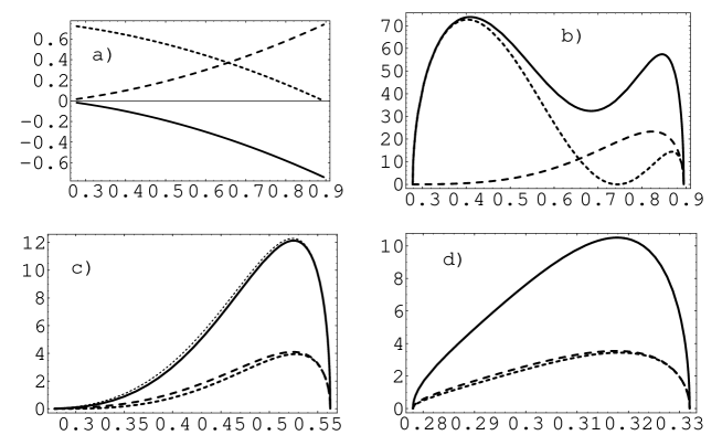
Figure 1: a) Born amplitudes with the ratio $g_{0}/g_{1}=3.11m_{1}^{2}$ and $g_{2}=g_{1}=1$ for the $\Upsilon_{31}$ mass relation. The solid line is the first term of $B^{(0,0)}$, the dotted line the second term, and the dashed line $-B^{(+.+)}$. b) The mass spectrum of $\Upsilon_{31}$ with $g_{2}/g_{1}=2$ and $g_{0}/g_{1}=3.11m_{1}^{2}$. The dotted line is the longitudinal helicity part, the dashed line the transverse helicity part, and the solid line the total cross section. c) $\Upsilon_{21}$ with the same $g_{0}$ and $g_{1}$ but with $g_{2}/g_{1}=0.1$. The dotted line near the solid line is the Voloshin-Zakharov formula with $\lambda=3.11$. d) $\Upsilon_{32}$ with the same $g_{2}/g_{1}$ but $g_{0}/g_{1}=2m_{1}^{2}$. The scales of all of the ordinates are arbitrary, and those of the abscissae are GeV.

Since the vector meson masses $M_{A}$ and $M_{B}$ are much larger than the maximum of the dipion mass, the coefficients of $(g_{1}s-g_{0})$ and $g_{2}$ are approximately equal to 1. We show the Born amplitudes in Fig. 1. Threshold suppression is realized under the condition $0\,<\,g_{0}/g_{1}\,<\,4m_{1}^{2}$ and $g_{2}=0$. We note that the Voloshin-Zakharov formula[6] is written $F\propto(s-\lambda m_{1}^{2})$ and the fitting the data gives $\lambda=3.11-3.42$.[24] The threshold rising and the double peak structure are obtained by adjusting $g_{1}$ and $g_{2}$. For example the choice $g_{2}/g_{1}=2$ gives the double peaks at about $W=0.44$ GeV and 0.85 GeV and the minimum at 0.68 GeV. The dominant contribution to the second peak comes from the transverse helicity amplitude, while the first peak is due to the longitudinal helicity ampitude.

Let us examine the total production amplitudes. As explained in the preceding section, the production amplitude is factorized into the Born and the rescattering terms;

$$F_{1}^{(\lambda,\lambda)}(s) = B^{(\lambda,\lambda)}(s)\cdot G_{1}(s),$$ (3.3)

$$G_{1}(s) = 1+J_{1}(s)T_{11}(s)+J_{2}(s)T_{21}(s),$$ (3.4)

where the $s\bar{s}$ production rate is taken to be the same as the $n\bar{n}$ one ($n=u$ and/or $d$), except for the mass difference between the pion and kaon, as in the scattering processes. $G_{i}(s)$ satisfies the same unitarity relation as the scalar form factor,

$${\rm Im}G_{i}(s)=-\sum_{j=1.2}G^{*}_{j}(s)\rho_{j}(s)T_{ji}(s),$$ (3.5)

and the rescattering correction without the kaon-loop,

$${\cal{S}}(s)=1+J_{1}(s)T_{11}(s),$$ (3.6)

is very similar to the existing scalar form factor such as that in Ref. 3), as shown in Fig. 2b). Thus, $G_{i}(s)$ could be regarded as an effective scalar form factor of the $i$-th dimeson channel. The absolute value $\left|G_{1}(s)\right|$ is rather flat for the mass range of the cascade decays as shown in Fig. 2a), and therefore the shapes of the mass distributions given by the Born terms are not so drastically altered.

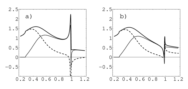
Figure 2: a) The effective form factor $G_{1}(s)$. The dashed line is the real part, the dotted line the imaginary part, and the solid line the absolute value. b) The pionic scalar form factor ${\cal{S}}(s)$. The identification of the lines is the same as in a).

Our model can reproduce the experimental data very well, as shown in Figs. 3a) - 3d), though these are not the best fits, where $g_{1}$ is chosen so as to normalize the calculated values to the experimental data. The values of $g_{n}$ are tabulated in Table I.

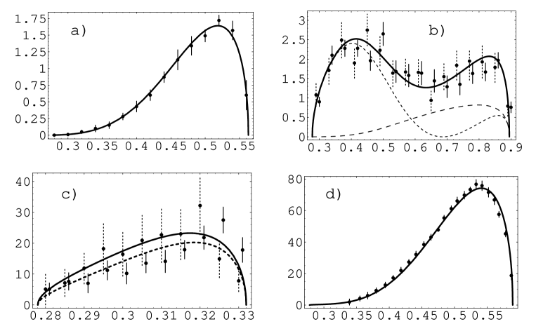
Figure 3: The invariant $\pi^{+}\pi^{-}$ mass spectra. The experimental data in a) - d) were read off of the figures of the published papers [1, 23, 24] by the present author. The solid and dashed error bars in b) and c) correspond to the exclusive and inclusive data, respectively. The scales of the ordinates are keV/GeV except for d), where it is events/0.01 GeV/c², and those of the abscissae are GeV. a) The mass spectrum of $\Upsilon_{21}$ with the data of Fig. 11 in Ref. 24). b) The mass spectra of $\Upsilon_{31}$ with the data of Fig.11 in Ref. 23). The dotted line is the longitudinal helicity part and the dashed line the transverse part. c) The mass spectra of $\Upsilon_{32}$ with the data of Fig.15 in Ref. 23). The lower line is for the ratio $g_{0}/g_{1}=2m_{1}^{2}$, and the upper line for the ratio $0$. The normalization of the upper and lower lines are different. d) The mass spectrum of $\psi_{21}$ with the data of Fig. 2(d) in Ref. 1).

Table 1: $g_{n}$ for Fig. 3. The left column of $\Upsilon_{32}$ corresponds to the lower dotted line and the right one does to the solid line.

$g_{n}$	$\Upsilon_{21}$	$\Upsilon_{31}$	$\Upsilon_{32}$		$\psi_{21}$
$g_{0}/g_{1}$	$3.11m_{\pi}^{2}$	$3.11m_{\pi}^{2}$	$2m_{\pi}^{2}$	$0m_{\pi}^{2}$	$3.42m_{\pi}^{2}$
$g_{2}/g_{1}$	0.1	1.25	0	0	0.2
$g_{1}$	7.29	3.65	$2.35\times 10^{2}$	$1.60\times 10^{2}$

For $\Upsilon_{21}$ and $\psi_{21}$, $g_{0}/g_{1}$ is required to be near to the value of Voloshin and Zakharov, and $g_{2}/g_{1}$ is required to be small. Then, we tentatively set $g_{0}/g_{1}=3.11m_{1}^{2}$ for $\Upsilon_{21}$ and $3.42m_{1}^{2}$ for $\psi_{21}$, and $g_{2}/g_{1}=0.1$ for $\Upsilon_{21}$ and $0.15$ for $\psi_{21}$. The small differences among them should not be taken seriously at present. In order to give the rapid rising at the threshold in $\Upsilon_{31}$, we need a large contribution from the $g_{2}$ term; we set $g_{2}/g_{1}=1.25$ with $g_{0}/g_{1}=3.11m_{1}^{2}$. The helicity structure of the double peaks is the same as in the Born approximation. The shape of $\Upsilon_{32}$ is rather sensitive to the value $g_{0}/g_{1}<2m_{1}^{2}$ under a small value of $g_{2}$. Since the difference between the experimental exclusive and inclusive data is not small, we try two cases that $g_{0}/g_{1}=2m_{1}^{2}$ and $0$ in Fig. 3c) It is seen that the values of the two coupling constant ratios do not deviate from those of the Born approximation, as stated above.

4 $J/\psi$ decays to $\phi(\pi\pi)$ and $\omega(\pi\pi)$

The experimental dipion mass spectrum of the final $\phi\pi\pi$ state is much different from that of the $\omega\pi\pi$ state; there is seen a clear peak of the $f_{0}(980)$ resonance in the former,[26] while we see a large broad peak centered at about 450 MeV and a small dip-bump structure at the $K\bar{K}$ threshold in the latter.[27] Since the charm quark lines annihilate and an $s\bar{s}$ or $n\bar{n}$ pair is created at the vector meson vertex in the $J/\psi$ decay into a light flavor vector meson, the validity of the spectator assumption is doubtful. Nevertheless, we use the same Lagrangian and the same model of the final state interaction, but we take account of the sequential decay process through the axial vector meson $b_{1}(1235)$, $J/\psi\to b_{1}\pi\to\omega(\pi\pi)$.

If we consider only the $g_{0}$ term as in Ref. 3), the resultant amplitudes are proportional to $G_{1}(s)$ for the $J/\psi\to\omega\pi\pi$ decay, and to $J_{2}(s)T_{21}$ for the $\phi\pi\pi$ decay. Both amplitudes, however, seem to give too large contributions in the $f_{0}(980)$ resonance region, so we introduce the $g_{1}$ term to reduce the contributions near 1 GeV. We tentatively use the parameter values, $g_{1}/g_{0}=0.7\,{\rm GeV}^{-2}$ and $g_{2}=0$. The overall normalization is controlled by the constant $g_{0}$. The Born terms in this parameter set generate a broad peak centered near 500 MeV and suppress the spectrum near 1 GeV for the $\omega\pi\pi$ decay, which are favorable effects for the model. However, they also produce another large peak near 2 GeV. It turns out, however, that the rescattering correction, $G_{1}(s)$, suppresses the second peak drastically, though the rescattering correction cannot be trusted at such higher energies. Thus, the validity of the model should be guaranteed for low energy $S$-wave production below 1.2 GeV or less, but the uniqueness of the parameters cannot be guaranteed.

4.1 $J/\psi\to\phi(\pi\pi)$

The dipion mass spectrum of this decay is similar to that of the radiative $\phi$ meson decay,[13], and the prominent peak is seen at about 1 GeV as the $f_{0}(980)$ resonance.[26] If the $\phi$ meson is the pure $s\bar{s}$ state, the direct $\pi\pi$ production accompanied by $\phi$ is the double OZI breaking vertex. The two channel production amplitudes with the lowest order OZI breaking vertex are, therefore, given as

$$F_{1}^{(\lambda,\lambda)}(s) = B^{(\lambda,\lambda)}(s)J_{2}(s)T_{21}(s),$$ (4.1)

$$F_{2}^{(\lambda,\lambda)}(s) = B^{(\lambda,\lambda)}(s)\left(1+J_{2}(s)T_{22}(s)\right),$$ (4.2)

where we notice that $F_{1}$ does not have the Born term.

If the double OZI breaking interaction is allowed, the above formula are modified as

$$F_{1}^{(\lambda,\lambda)}(s) = B^{(\lambda,\lambda)}\left(J_{2}T_{21}+\alpha(1+J_{1}T_{11})\right),$$ (4.3)

$$F_{2}^{(\lambda,\lambda)}(s) = B^{(\lambda,\lambda)}(s)\left(1+J_{2}(s)T_{22}(s)+\alpha J_{1}(s)T_{12}(s)\right)$$ (4.4)

where $\alpha$ denotes an additional OZI breaking rate. The calculated result on the $\pi^{+}\pi^{-}$ invariant mass spectrum is given in Fig. 4, where we set $\alpha=0.2$, and the overall normalization is fixed at the $f_{0}(980)$ peak. If the double OZI breaking interaction is forbidden, that is $\alpha=0$, the small enhancement disappears. The too steep rising of the $\pi\pi$ mass spectrum at the $f_{0}(980)$ resonance is due to the defect of our $T_{11}(s)$ given in Ref. 19), where the phase shift $\delta_{00}$ increases too rapidly near the $K\bar{K}$ threshold. This defect also induces a too sharp and large peak in $T_{12}$.

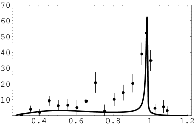
Figure 4: The $\pi^{+}\pi^{-}$ mass spectrum for $\alpha=0.2$. The experimental data were read off of Fig. 7 in Ref. 3), where the scale of the ordinate is events/25 MeV.

4.2 $J/\psi\to\omega(\pi\pi)$

While the branching ratio of $J/\psi\to\omega\pi^{+}\pi^{-}$ is $(7.2\,\pm\,1.0)\times 10^{-3}$ and that of $\omega\pi^{0}\pi^{0}$ $(3.4\pm 0.8)\times 10^{-3}$, the ratio of $J/\psi\to b_{1}^{\pm}(1235)\pi^{\mp}$ is $(3.0\,\pm\,0.5)\times 10^{-3}$ and that of $b_{1}^{0}(1235)\pi^{0}$ $(2.3\pm 0.6)\times 10^{-3}$, according to the PDG data.[4] This implies that the sequential decay $J/\psi\to b_{1}\,\pi\to\omega\,\pi\pi$ cannot be ignored. We include both the direct $\omega\,\pi\pi$ decay and the sequential decay process in the analysis.

The direct production amplitude is given under the same spectator hypothesis as

$$F_{\rm dir}^{(\lambda,\lambda)}(s)=B^{(\lambda,\lambda)}(s)\left(1+J_{1}(s)T_{11}(s)+J_{2}(s)T_{21}(s)\right),$$ (4.5)

where we note that $K\bar{K}$ production accompanied by $\omega$ does not further break the OZI rule. We show the mass spectra obtained from the direct production amplitude in Figs. 5a) and b) by the dotted lines. They are identical except for the normalization. The spectrum shows a broad peak near 450 MeV and the up-down structure near the $K\bar{K}$ threshold.

The sequential decay amplitude is calculated as follows: We set the effective Lagrangian to describe the vertices $J/\psi\to b_{1}\pi$ and $b_{1}\to\omega\pi$ as

$$L_{\rm int}=g_{\psi b_{1}\pi}\psi_{\mu}b_{i}^{\mu}\pi_{i}(x)+g_{b_{1}\omega\pi}\omega_{\mu}b^{\mu}_{i}\pi_{i}(x),$$ (4.6)

where $\psi_{\mu}(x)$($b_{i}^{\mu}(x)$, $\omega_{\mu}(x)$) is the $J/\psi$($b_{1}$, $\omega$) field, and we assume that both of the decays arise through a pure $S$-wave at the rest frame of the mother particle. We write the Born term for the sequential decay as

$$B_{\rm seq}=g_{\psi b_{1}\pi}g_{b_{1}\omega\pi}\left\{\frac{(\epsilon_{\omega}^{*}\epsilon_{b})(\epsilon_{b}^{*}\epsilon_{\psi})}{P_{b}^{2}-M_{b}^{2}+iM_{b}\Gamma_{b}}+\frac{(\epsilon_{\omega}^{*}\epsilon_{b})(\epsilon_{b}^{*}\epsilon_{\psi})}{{P^{\prime}_{b}}^{2}-M_{b}^{2}+iM_{b}\Gamma_{b}}\right\},$$ (4.7)

where $M_{b}$ and $\Gamma_{b}$ are the mass and total width of $b_{1}$, and

$$P_{b} = p_{\psi}-q_{2}=p_{\omega}+q_{1},$$ (4.8)

$$P^{\prime}_{b} = p_{\psi}-q_{1}=p_{\omega}+q_{2}.$$ (4.9)

Summing the helicities of the intermediate $b_{1}$ meson, we have

$$B^{(\lambda,\lambda)}_{\rm seq}(s,z) = g_{0}R\left\{\frac{N^{(\lambda,\lambda)}(s,z)}{D(s,z)}+\frac{N^{(\lambda,\lambda)}(s,-z)}{D(s,-z)}\right\},$$ (4.10)

$$D(s,z) = \frac{M_{\psi}^{2}+M_{\omega}^{2}-s+2m_{1}^{2}}{2}-M_{b}^{2}+iM_{b}\Gamma_{b}-2pqz,$$ (4.11)

$$N^{(\lambda,\lambda)}(s,z) = -\left[({\epsilon_{\omega}^{(\lambda)}}^{*}\cdot\epsilon_{\psi}^{(\lambda)})+(\epsilon_{\omega}^{(\lambda)}\cdot q_{1})^{*}(\epsilon_{\psi}^{(\lambda)}\cdot q_{2})/M_{b}^{2}\right]$$ (4.12)

with $R=g_{\psi b_{1}\pi}g_{b_{1}\omega\pi}/g_{0}$. The sequential decay amplitude includes the $D$-wave contribution, but we calculate only the $S$-wave part in the Born approximation in this paper.

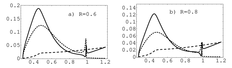
Figure 5: The $\pi^{+}\pi^{-}$ mass spectrum. The left side is the results for the relative ratio $R=0.6$, and the right for $R=0.8$. The spectra calculated with the total amplitude are given by the solid lines, those with the pure direct production amplitude by the dotted lines, and those with the sequential decay term by the dashed lines. The scale of the ordinate is keV/GeV, using the value of $g_{0}$ estimated as explained in the text.

The mass spectrum is calculated with the total amplitude,

$$F_{\rm tot}^{(\lambda,\lambda)}=F_{\rm dir}^{(\lambda,\lambda)}+B_{\rm seq}^{(\lambda,\lambda)}|_{S},$$ (4.13)

where the second term is the $S$-wave part of the sequential Born term. It should be noted that the tolal amplitude does not satisfy exact unitarity, since the sequential decay amplitude is within the Born approximation. If we compare the decay widths $J/\psi\to(b_{1}\pi)_{I=0}$ and $b_{1}\to\omega\pi$ calculated in the Born approximation with the experimental data, we can estimate the product of the two coupling constants as $g_{\psi b_{1}\pi}g_{b_{1}\omega\pi}=2.53\times 10^{-2}\,{\rm GeV}^{2}$, where we take ${\rm Br}(J/\psi\to(b_{1}\pi)_{I=0})=5.3\times 10^{-3}$ and the $S$-wave partial width of $b_{1}$ as $\Gamma_{S}(b_{1}\to\omega\pi)=100$ MeV.[4] Setting $R=0.6$, then, gives $g_{0}=4.22\times 10^{-2}\,{\rm GeV}^{2}$, and $R=0.8$ gives $1.78\times 10^{-2}\,{\rm GeV}^{2}$. We show the mass spectra calculated with the model using the estimated coupling constants in Fig. 5, but we do not compare the calculated mass spectrum with the experimental data, because the data include the $D$-wave contribution which could not be disregarded above 500 MeV. From Fig. 5 we observe that the $S$-wave mass distribution shows a large peak at about 450 MeV, small structure at the $f_{0}(980)$ resonance and increasing behavior of the sequential decay, all of which are consistent with the experimental data.[27] We also see that the interference between the two amplitudes cannot be ignored, but the inclusion of the final state interaction in the sequential decay may alter the pattern of the interference.

5 Concluding remarks

We have demonstrated the validity of our phenomenological model in describing the mass spectra of the dipion states produced in heavy flavor vector meson decays. We have shown that the model describes the mass spectra very well with two ratios of the three coupling constants, and an overall normalization. The model takes account of the final state interaction between the produced dipion state through the two-point loop integral familiar to ChPT and the two-channel $S$-wave scattering amplitudes given by the unitarized chiral theory. The form of the total production amplitudes in our model is not proportional to the scattering amplitudes, as in the so-called universal hypothesis, nor independent of the scattering processes. The model does not need the Breit-Wigner formula for the bump at 500 MeV and the $f_{0}(980)$ resonance, neither of which is a preexisting meson state but, rather, dynamical objects emerging from the multichannel scattering dynamics. The fact that the $f_{0}(980)$ peak is more clearly seen in production processes than scattering processes is due to the large coupling of the $f_{0}(980)$ state with the $K\bar{K}$ channel. Such a special effect is not expected for the $\sigma$ state, because the $K\bar{K}\to\pi\pi$ amplitude in this region does not have any enhancement. We conclude that these decay processes cannot be more useful in revealing the nature of the $\sigma$ state than scattering processes deduced from the peripheral production processes. We again emphasize that the $I=J=0$ $\pi\pi$ scattering amplitude obtained in the unitarized chiral theory generates the broad peak near 500 MeV without a preexisting $\sigma$ field expressed by the Breit-Wigner formula.[19]

Although we reproduced the experimental data well, it is impossible to predict the variety of the ratios of the coupling constants and the overall normalization constants within our phenomenological model. The process dependence of the parameters could be analyzed through complicated QCD calculations, but this is far beyond our scope.

The angular distribution of $\mbox{\boldmath$q$}_{1}$ in the $Q$-frame indicates that the dipion state is not a pure $S$-wave state for $\Upsilon_{21}$ and $\Upsilon_{31}$.[23, 24] This is also the case for $J/\psi\to\omega\pi\pi$,[27] where the angular distribution for $W\,>\,600$ MeV shows a significant angle dependence like a $D$-wave contamination. As pointed out in §4, the $D$-wave component of the sequential decay $J/\psi\to b_{1}(1235)\pi\to\omega\pi\pi$ would contribute substantially to the large tail of the $f_{2}(1270)$ resonance.

We do not consider the calculation of the $K\bar{K}$ spectra in this paper, because there are ambiguous contamination of multiple sequential decays such as $J/\psi\to K^{*}(1270)\bar{K}+{\rm c.c.}$ and $K^{*}(1400)\bar{K}+{\rm c.c.}$ for both of the final states, $\phi K\bar{K}$ and $\omega K\bar{K}$. According to the PDG data[4] the branching ratios are $<\,3.0\times 10^{-3}$ for the former and $(3.8\pm 1.4)\times 10^{-3}$ for the latter decay channel. Neither of the axial vector mesons can decay into the $\phi K$ state, but they can couple to it. The pure direct decay component gives rapid threshold rising and then decreasing behavior in the $K\bar{K}$ mass distribution. This is due to the peak behavior of $T_{22}$ near the $K\bar{K}$ threshold owing to the $f_{0}(980)$ state. Similar threshold rising behavior is seen in $\gamma\gamma\to K\bar{K}$ and $\phi\to\gamma K^{0}\bar{K}^{0}$.[13]

References

- [1] T. Komada, M. Ishida and S. Ishida, Phys. Lett. B508 (2001), 31.
- [2] M. Ishida, S. Ishida, T. Komada and S-I. Matsumoto, Phys. Lett. B518 (2001), 47.
- [3] Ulf-G. Meissner and J.A. Oller, Nucl. Phys. A679 (2001), 671.
- [4] K. Hagiwara et al., Phys. Rev. D66 (2002), 010001.
- [5] K. L. Au, D. Morgan and M. R. Pennington, Phys. Rev. D35 (1987), 1633.
- [6] M. Voloshin an V. Zakharov, Phys. Rev. Lett. 45 (1980), 688.
- [7] V. A. Novikov and M. A. Shifman, Z. Phys. C 8 (1981), 43.
- [8] T.-M. Yan, Phys. Rev. D22 (1980), 1652.
- [9] G. Bélanger, T. DeGrand and P. Moxhay, Phys. Rev. D 39 (1987), 257.
- [10] H. J. Lipkin and S. F. Tuan, Phys. Lett. B206 (1988), 349.
- [11] P. Moxhay, Phys. Rev. D39 (1989), 3497.
- [12] H.-Y Zhou and Yu-P. Kuang, Phys. Rev. D44 (1991), 756.
- [13] M. Uehara, hep-ph/0206141.
- [14] J. A. Oller and E. Oset, Nucl. Phys. A629 (1998), 739.
- [15] E. Marco, S. Hirenzaki, E, Oset and H. Toki, Phys. Lett. B470 (1999), 20.
-
[16]
A. Dobado and J. R. Pelàez, Phys. Rev. D56 (1997), 3057.
T. Hanna, Phys. Rev. D54 (1996), 4654; ibid. D55 (1997), 5613.
A. Goméz Nicola and J. R. Pelàez, Phys. Rev. D65 (2002), 054009. -
[17]
J. A. Oller and E. Oset, Nucl. Phys. A620 (1997), 438;
Errata Nucl. Phys. A652 (1999), 407. -
[18]
J. A. Oller, E. Oset and J. R. Pelàez, Phys. Rev. D59 (1999), 0074001;
Errata Phys. Rev. D60 (1999), 09906. - [19] M. Uehara, hep-ph/0204020.
- [20] Ulf-G. Meissner, Comm. Nucl. Part. Phys. 20 (1991), 119.
- [21] G. Colangele, J. Gasser and H. Leutweyler, Nucl. Phys. B603 (2001), 125.
- [22] S. Gardner and Ulf-G. Meissner, Phys. Rev. D65 (2002), 094004.
- [23] F. Butler et al., Phys. Rev. D49 (1994),40.
- [24] J. P. Alexander et al., Phys. Rev. D58 (1999), 052004.
- [25] M. Oreglia et al., Phys. Rev. Lett. 45 (1980), 959.
- [26] A. Falvard et al., Phys. Rev. D38 (1988), 2706.
- [27] J. E. Augstin et al., Nucl. Phys. B320 (1989), 1;