BNL-NT-02/23

RBRC-293

October 2002

Next-to-leading order QCD corrections

to high-$\mathbf{p_{T}}$ pion production in

longitudinally polarized $\mathbf{pp}$ collisions

B. Jäger^a, A. Schäfer^a, M. Stratmann^a, and W. Vogelsang^b,c

^aInstitut für Theoretische Physik, Universität Regensburg,
D-93040 Regensburg, Germany

^bPhysics Department, Brookhaven National Laboratory,
Upton, New York 11973, U.S.A.

^cRIKEN-BNL Research Center, Bldg. 510a, Brookhaven National Laboratory,
Upton, New York 11973 – 5000, U.S.A.

We present a calculation for single-inclusive large-$p_{T}$ pion production in longitudinally polarized $pp$ collisions in next-to-leading order QCD. We choose an approach where fully analytical expressions for the underlying partonic hard-scattering cross sections are obtained. We simultaneously rederive the corresponding corrections to unpolarized scattering and confirm the results existing in the literature. Our results allow to calculate the double-spin asymmetry $A_{LL}^{\pi}$ for this process at next-to-leading order, which will soon be used at BNL-RHIC to measure the polarization of gluons in the nucleon.

1 Introduction

The measurement of the proton’s spin-dependent deep-inelastic structure function $g_{1}^{p}$ by the EMC [1] more than a decade ago made once again the spin structure of the nucleon an exciting topic, which deservedly continues to spark large activity by both theorists and experimentalists. The original result, that the total quark spin contribution to the nucleon spin is only of the order of about $20\%$ has subsequently been confirmed by other experiments and is well-established today. For various reasons that we will not review here, gluons may very well play a more important role for the proton spin than quarks. Consequently, there is now a flurry of experimental activity aiming at measuring the polarization of gluons in the nucleon. In terms of a parton density, the required information is contained in [2]

$$\Delta g\left(x,\mu_{F}\right)\,=\,\frac{i}{4\pi\,x\,P^{+}}\int d\lambda\,{\rm e}^{i\lambda xP^{+}}\,\langle P,S|G^{+\nu}(0)\,\tilde{G}^{+}_{\;\;\nu}(\lambda n)|P,S\rangle\Big{|}_{\mu_{F}}\;\;,$$ (1)

written in $A^{+}=0$ gauge, where $x$ is the gluon’s light-cone momentum fraction of the proton momentum $P^{+}$, and $\mu_{F}$ the factorization scale appearing in a hard process to which the gluon contributes. $G^{\mu\nu}$ is the field strength tensor, and $\tilde{G}^{\mu\nu}$ its dual. In more simple terms, $\Delta g(x,\mu_{F})$ describes the difference in probabilities for finding a gluon with positive or negative helicity in a proton with positive helicity, at “resolution” scale $\mu_{F}$:

$$\Delta g(x,\mu_{F})\equiv g_{+}^{+}(x,\mu_{F})-g_{-}^{+}(x,\mu_{F})\;,$$ (2)

where superscripts (subscripts) denote the proton (gluon) helicity.

Deeply-inelastic scattering (DIS), $lp\to l^{\prime}X$, is a standard process for studying nucleon structure. However, it is not an ideal process for measuring the gluon content of the nucleon, due to the fact that the virtual photon in DIS couples directly only to quarks. Inclusive structure functions therefore depend on the gluon density only through scale-evolution, and through higher orders in QCD perturbation theory. This explains why the existing polarized-DIS data have told us very little about $\Delta g$ [3, 4]. One may attempt to get access to the gluon density by selecting the photon-gluon-fusion process in DIS, which contributes to final states such as heavy flavor pairs, or high-transverse momentum ($p_{T}$) hadron pairs. Indeed, the Compass experiment [5] at CERN and Hermes [6] at DESY follow this approach. Unfortunately, the rather low energy in these fixed-target experiments and the ensuing large systematic uncertainties in the theoretical predictions complicate these efforts significantly. Dedicated experiments at a possibly forthcoming future polarized $ep$ collider, like the EIC [7], would presumably make these channels more promising, however.

The BNL Relativistic Heavy-Ion Collider RHIC [8] is able to run in a mode with polarized protons. Very inelastic $pp$ collisions will then open up unequaled possibilities to measure $\Delta g$. RHIC has the advantage of operating at high energies ($\sqrt{S}=200$ and $500$ GeV), where the theoretical description is under good control. In addition, it offers various different channels in which $\Delta g$ can be studied, such as prompt photon production, jet production, creation of heavy flavor pairs, or inclusive-hadron production. In this way, RHIC is expected to provide the best source of information on $\Delta g$ for a long time to come.

The basic concept that underlies most of spin physics at RHIC is the factorization theorem [9], which states that large momentum-transfer reactions may be factorized into long-distance pieces that contain the desired information on the (spin) structure of the nucleon in terms of its parton densities such as $\Delta g(x,\mu_{F})$, and parts that are short-distance and describe the hard interactions of the partons. The two crucial points here are that on the one hand the long-distance contributions are universal, i.e., they are the same in any inelastic reaction under consideration, and that on the other hand the short-distance pieces depend only on the large scales related to the large momentum transfer in the overall reaction and, therefore, can be evaluated using QCD perturbation theory. The factorized structure forces one to introduce into the calculation a scale of the order of the hard scale in the reaction – but not specified further by the theory – that separates the short- and long-distance contributions. This scale is the factorization scale $\mu_{F}$ mentioned above.

As an example, let us consider the spin-dependent cross section for the reaction $pp\to\pi X$, where the pion is at high transverse momentum, ensuring large momentum transfer. This is the reaction we study in the following. The spin-dependent differential cross section is defined as

$$d\Delta\sigma\equiv\frac{1}{2}\left[d\sigma^{++}-d\sigma^{+-}\right]\;\;,$$ (3)

where again the superscripts denote the helicities of the protons in the scattering. The statement of the factorization theorem is then:

$$d\Delta\sigma = \sum_{a,b,c}\,\int dx_{a}\int dx_{b}\int dz_{c}\,\,\Delta f_{a}(x_{a},\mu_{F})\,\Delta f_{b}(x_{b},\mu_{F})D_{c}^{\pi}(z_{c},\mu_{F}^{\prime})\,$$ (4)

$$\times\,d\Delta\hat{\sigma}_{ab}^{c}(x_{a}P_{A},x_{b}P_{B},P_{\pi}/z_{c},\mu_{R},\mu_{F},\mu_{F}^{\prime})\;\;,$$

where the sum is over all contributing partonic channels $a+b\to c+X$, with $d\Delta\hat{\sigma}_{ab}^{c}$ the associated partonic cross section, defined in complete analogy with Eq. (3), the helicities now referring to partonic ones:

$$d\Delta\hat{\sigma}_{ab}^{c}\equiv\frac{1}{2}\Bigg{[}\left(d\hat{\sigma}_{ab}^{c}\right)^{++}-\left(d\hat{\sigma}_{ab}^{c}\right)^{+-}\Bigg{]}\;\;.$$ (5)

A few further comments are in order here. First, Eq. (4) is actually a slight extension of the factorization theorem compared to what we stated above: the fact that we are observing a specific hadron in the reaction requires the introduction of additional long-distance functions, the parton-to-pion fragmentation functions $D_{c}^{\pi}$. These functions have been determined with some accuracy by observing leading pions in $e^{+}e^{-}$ collisions and in DIS. Even though there is certainly room for improvement in our knowledge of the $D_{c}^{\pi}$, we assume for this study that the fragmentation functions are sufficiently known.

Secondly, we have displayed the full set of required scales in Eq. (4). Besides the factorization scale $\mu_{F}$ for the initial-state partons, there is also a factorization scale $\mu_{F}^{\prime}$ for the absorption of long-distance effects into the fragmentation functions. In addition, we have a renormalization scale $\mu_{R}$ associated with the running strong coupling constant $\alpha_{s}$.

As mentioned above, the partonic cross sections may be evaluated in perturbation theory. Schematically, they can be expanded as

$$d\Delta\hat{\sigma}_{ab}^{c}\,=\,d\Delta\hat{\sigma}_{ab}^{c,(0)}+\frac{\alpha_{s}}{\pi}d\Delta\hat{\sigma}_{ab}^{c,(1)}+\ldots\;.$$ (6)

$d\Delta\hat{\sigma}_{ab}^{c,(0)}$ is the leading-order (LO) approximation to the partonic cross section and is, for our case of pion production, obtained from evaluating all basic $2\to 2$ QCD scattering diagrams. It is therefore of order $\alpha_{s}^{2}$. The lowest order, however, can generally only serve to give a rough description of the reaction under study. It merely captures the main features, but does not usually provide a quantitative understanding. The first-order (“next-to-leading order” [NLO]) corrections are generally indispensable in order to arrive at a firmer theoretical prediction for hadronic cross sections. For instance, the dependence on the unphysical factorization and renormalization scales is expected to be much reduced when going to higher orders in the perturbative expansion. Only with knowledge of the NLO corrections can one reliably extract information on the parton distribution functions from the reaction. This is true, in particular, for spin-dependent cross sections, where both the polarized parton densities and the polarized partonic cross sections may have zeros in the kinematical regions of interest, near which the predictions at lowest order and the next order will show marked differences.

There has been a lot of effort in recent years [10-15] to obtain the NLO corrections for the spin-dependent cross sections most relevant for the RHIC spin program. By now, essentially the only remaining uncalculated corrections are those for the partonic cross sections in Eq. (4), i.e., inclusive pion production. These corrections will be presented in this paper. We emphasize that it is very appropriate to provide the NLO corrections at this time: it is planned for the coming RHIC run (early 2003) to attempt a first measurement of $\Delta g$ through exactly the spin asymmetry

$$A_{LL}^{\pi}=\frac{d\Delta\sigma}{d\sigma}=\frac{d\sigma^{++}-d\sigma^{+-}}{d\sigma^{++}+d\sigma^{+-}}$$ (7)

for high-$p_{T}$ pion production. The main underlying idea here is that $A_{LL}^{\pi}$ is very sensitive to $\Delta g$ through the contributions from polarized quark-gluon and gluon-gluon scatterings. We note that the Phenix collaboration has recently presented first, still preliminary, results for the unpolarized cross section for $pp\to\pi^{0}X$ at $\sqrt{S}=200$ GeV, which are well described by the NLO QCD calculation [16], providing confidence that the theoretical framework based on perturbative-QCD hard scattering and summarized by Eq. (4) is adequate.

Section 2 gives an outline of the calculation, summarizing the main ingredients. In Sec. 3 we present some first numerical applications of our results.

2 Calculation of the NLO corrections

2.1 Outline of the strategy of the calculation

The “parton-model” type picture employed in Eq. (4) implies that the partonic cross sections $d\Delta\hat{\sigma}_{ab}^{c}$ are single-inclusive cross sections for the reactions $a+b\to c+X$, i.e., summed over all final states (excluding $c$) possible at the order considered, and integrated over the entire phase space of $X$. Writing out Eq. (4) explicitly to NLO, we have

$$E_{\pi}\frac{d\Delta\sigma}{d^{3}p_{\pi}} = \frac{1}{\pi S}\sum_{a,b,c}\int^{1}_{z_{0}}\frac{dz_{c}}{z_{c}^{2}}\int_{VW/z_{c}}^{1-(1-V)/z_{c}}\!\!\!\frac{dv}{v(1-v)}\int^{1}_{VW/vz_{c}}\!\!\frac{dw}{w}\Delta f_{a}(x_{a},\mu_{F})\Delta f_{b}(x_{b},\mu_{F})D_{c}^{\pi}(z_{c},\mu_{F}^{\prime})$$ (8)

$$\times \,\left[\frac{d\Delta\hat{\sigma}^{c,(0)}_{ab}(v)}{dv}\delta(1-w)+\frac{\alpha_{s}(\mu_{R})}{\pi}\,\frac{d\Delta\hat{\sigma}^{c,(1)}_{ab}(s,v,w,\mu_{R},\mu_{F},\mu_{F}^{\prime})}{dvdw}\right]\;\;,$$

where $z_{0}=1-V+VW$, with hadron-level variables

$$V\equiv 1+\frac{T}{S}\;\;,\;\;\;\;W\equiv\frac{-U}{S+T}\;\;,\;\;\;\;S\equiv(P_{A}+P_{B})^{2}\;\;,\;\;\;\;T\equiv(P_{A}-P_{\pi})^{2}\;\;,\;\;\;\;U\equiv(P_{B}-P_{\pi})^{2}\;\;,$$ (9)

and corresponding partonic ones

$$v\equiv 1+\frac{t}{s}\;\;,\;\;\;\;w\equiv\frac{-u}{s+t}\;\;,\;\;\;\;s\equiv(p_{a}+p_{b})^{2}\;\;,\;\;\;\;t\equiv(p_{a}-p_{c})^{2}\;\;,\;\;\;\;u\equiv(p_{b}-p_{c})^{2}\;\;.$$ (10)

Neglecting all masses, one has the relations

$$s=x_{a}x_{b}S\;\;,\;\;\;\;t=\frac{x_{a}}{z_{c}}T\;\;,\;\;\;\;u=\frac{x_{b}}{z_{c}}U\;\;,\;\;\;x_{a}=\frac{VW}{vwz_{c}}\;\;,\;\;\;\;x_{b}=\frac{1-V}{z_{c}(1-v)}\;\;.$$ (11)

The LO partonic cross sections $d\Delta\hat{\sigma}^{c,(0)}_{ab}(v)$ are calculated from the $2\to 2$ QCD scattering processes, that is, $X$ consists of only one parton, and its phase space is trivial and leads to the $\delta(1-w)$ factor in Eq. (8). We do not need to present the cross sections here, which have been known for a long time for both the unpolarized and the polarized cases [17]. There are actually only four generic reactions, $qq^{\prime}\to qq^{\prime}$, $qq\to qq$, $q\bar{q}\to gg$, and $gg\to gg$; all other processes follow from crossing if one works in terms of helicity amplitudes for each reaction, keeping all particles polarized. All tree-level $2\to 2$ helicity amplitudes are given in [18]. The four generic processes give rise to the ten separate LO channels

$$qq^{\prime} \to qX$$

$$q\bar{q}^{\prime} \to qX$$

$$q\bar{q} \to q^{\prime}X$$

$$qq \to qX$$

$$q\bar{q} \to qX$$

$$q\bar{q} \to gX$$

$$qg \to qX$$

$$qg \to gX$$

$$gg \to gX$$

$$gg \to qX\;,$$ (12)

the “observed” final-state parton fragmenting into the hadron. At NLO, we have ${\cal O}(\alpha_{s})$ corrections to the above reactions, and also the additional new processes

$$qq^{\prime} \to gX$$

$$q\bar{q}^{\prime} \to gX$$

$$qq \to gX$$

$$qg \to q^{\prime}X$$

$$qg \to \bar{q}^{\prime}X$$

$$qg \to \bar{q}X\;.$$ (13)

A single-inclusive-parton cross section is, of course, not a priori infrared-finite in QCD, but sensitive to long-distance dynamics through the presence of collinear singularities that arise when the momenta of partons in the initial or final states become parallel. Such a situation can appear for the first time at ${\cal O}(\alpha_{s}^{3})$ (NLO), where $2\to 3$ scattering diagrams contribute. From the factorization theorem discussed above it follows that long-distance sensitive contributions may be factored into the bare parton distribution functions or fragmentation functions. The result of this procedure are finite partonic hard-scattering cross sections $d\Delta\hat{\sigma}_{ab}^{c}$. At intermediate stages, however, the calculation will necessarily show singularities that represent the long-distance sensitivity. In addition, for those processes that are already present at LO, real $2\to 3$ and virtual one-loop $2\to 2$ diagrams contributing to the calculation will individually have infrared singularities that only cancel in their sum. Virtual diagrams will also produce ultraviolet poles that need to be removed by the renormalization of the strong coupling constant at a scale $\mu_{R}$. As a result, a regulator has to be introduced into the calculation that makes all the singularities manifest so that they can be canceled in the appropriate way. Our choice will be dimensional regularization, that is, the calculation will be performed in $d=4-2\varepsilon$ space-time dimensions. Subtractions of singularities will generally be made in the $\overline{\rm{MS}}$ scheme.

Dimensional regularization becomes a somewhat subtle issue if polarizations of particles are taken into account. This is due to the fact that projections on helicities involve the Dirac matrix $\gamma_{5}$ for quarks and the Levi-Civita tensor $\epsilon^{\mu\nu\rho\sigma}$ for gluons. These two objects are genuinely four-dimensional and hence do not have a natural extension to $4-2\varepsilon$ dimensions. In fact, some care has to be taken to avoid algebraic inconsistencies in the calculation when using $\gamma_{5}$ and $\epsilon^{\mu\nu\rho\sigma}$. At the level of the algebra the treatment of $\gamma_{5}$ and $\epsilon^{\mu\nu\rho\sigma}$ of course only affects terms that are of ${\cal O}(\varepsilon)$. However, poles proportional to $1/\varepsilon$ and $1/\varepsilon^{2}$ present in the calculation may combine with this to eventually result in non-vanishing contributions. A widely-used scheme for dealing with $\gamma_{5}$ and $\epsilon^{\mu\nu\rho\sigma}$ in a fully consistent way is the one developed in [19], the HVBM scheme. This is the scheme we have used for our calculation. It is mainly characterized by splitting the $d$-dimensional metric tensor into a four-dimensional and a $(d-4)$-dimensional one. The Levi-Civita tensor is then defined by having components within the four-dimensional subspace only, and $\gamma_{5}$ anti-commutes with the other Dirac matrices in the four-dimensional subspace, but commutes with them in the $(d-4)$-dimensional one. The HVBM scheme leads to a higher complexity of the algebra and of phase space integrals. However, one may make use of computer algebra programs such as Tracer [20] that allow to handle the split-up of space-time, and the treatment of $(d-4)$-dimensional components in phase space integrals has become rather standard by now. We emphasize that for our present case the treatment of $\gamma_{5}$ and $\epsilon^{\mu\nu\rho\sigma}$ has no bearing on the ultraviolet (renormalization) sector of the calculation, since we have no chiral vertices in the calculation. For instance, we may perform all renormalizations at the level of vertex and self-energy diagrams, without reference to the polarizations of the external particles.

As remarked above, we need to sum over all possible final states in each channel $ab\to cX$, in compliance with the requirement of single-inclusiveness of the cross section. For instance, in case of $qg\to qX$ one needs, besides the virtual corrections to $qg\to qg$, three different $2\to 3$ reactions: $qg\to q(gg)$, $qg\to q(q\bar{q})$, $qg\to q(q^{\prime}\bar{q}^{\prime})$ (where brackets indicate the unobserved parton pair). Only all three processes combined will allow to arrive at a finite answer in the end. The summation over $X$ is therefore always implicitly understood in the following.

In addition, the two unobserved partons in the $2\to 3$ contributions need to be integrated over their entire phase space. The integration may be performed in basically two different ways. The first one relies on Monte-Carlo integration techniques. As was shown in [21, 22], the regions where the squared $2\to 3$ matrix elements become singular can be straightforwardly identified and separated. These regions will yield all the poles in $1/\varepsilon$ after integration, which eventually must cancel as described above. It then becomes possible to organize the calculation in such a way that the singularities are extracted and canceled by hand, while the remainder may be integrated numerically over phase space. This approach has the advantage of being very flexible; it may be used for any infrared-safe observable, with any experimental cut [21]. On the other hand, the numerical integration involved turns out to be rather delicate and time-consuming. In case of polarized collisions, the method was employed for the reactions $pp\to{\rm jet}X$ [13] and $pp\to\gamma X$ [12] at NLO.

The method we will employ is to perform the phase space integration of the $2\to 3$ contributions analytically. This has several advantages. In first place, the final answer is much more amenable to a numerical evaluation, giving much more stable results in a much shorter time. This may become important at a later stage, when experimental data will have been obtained and one is aiming to extract $\Delta g$ from them within a “global analysis” [23]. In addition, the “analytic method” has also been employed in the unpolarized case [24]. Since the calculation of the unpolarized and the polarized NLO terms largely proceeds along similar lines, we can compute both simultaneously. Our results for the unpolarized case may then be compared at an analytical level to those available in the numerical code of [24], which provides an extremely powerful check on the correctness of all our calculations.

We will now separately address the virtual $2\to 2$ and real-emission $2\to 3$ NLO contributions. Then we will discuss their sum and the cancellation of singularities.

2.2 Virtual contributions

At ${\cal O}(\alpha_{s}^{3})$, virtual corrections only contribute through their interference with the Born diagrams, as sketched in Fig. 1. We have calculated the virtual contributions with two different methods.

Figure 1: Interference of generic virtual (box, vertex, self-energy) contributions with Born diagrams.

Firstly, we have performed a direct calculation. Here we could make use of known $\overline{\rm{MS}}$-renormalized one-loop vertex and self-energy structures as given in [25], which may be readily inserted into the Born diagrams. One then additionally needs to calculate the box diagrams which are ultraviolet finite and hence not subject to the renormalization procedure. We have simultaneously computed the virtual corrections for the unpolarized case and found complete agreement with the results published in [26].

The second approach makes use of the fact that in Ref. [27] the helicity amplitudes for all one-loop $2\to 2$ QCD scattering diagrams were presented. It is clear that these contain the information we need for our calculation. The only subtlety is that the helicity method employed in [27] will not immediately yield the answer for the HVBM prescription we are looking for. However, as was also pointed out in [22, 27], the translation between the results for the two schemes is fairly straightforward. In fact, by inspecting the singularity structure of the diagrams, one can derive a universal form for the virtual contribution ${\cal V}$ that schematically reads:

$${\cal V}(s,t,u)={\cal B}(s,t,u)\left\{-\frac{1}{\varepsilon^{2}}\sum_{n}C_{n}-\frac{1}{\varepsilon}\sum_{n}\gamma_{n}\right\}+\frac{1}{\varepsilon}\sum_{m<n}\log\left(\frac{2p_{n}\cdot p_{m}}{s}\right)\tilde{{\cal B}}_{mn}(s,t,u)+\tilde{{\cal V}}(s,t,u),$$ (14)

where $n,m$ are summed over all external legs, the $p_{i}$ are the external parton momenta, and ${\cal B}$ denotes the Born cross section for the reaction under consideration. The $\tilde{{\cal B}}_{mn}$ are the so-called “color-linked” Born cross sections, to be calculated according to rules given in [22]. The $C_{i}$ and $\gamma_{i}$ are coefficients depending only on the type of external leg, with $C_{q}=C_{F}=4/3$, $C_{g}=C_{A}=3$, $\gamma_{q}=3C_{F}/2$, $\gamma_{g}=\beta_{0}/2=11/2-n_{f}/3$, $n_{f}$ being the number of flavors. Finally, $\tilde{{\cal V}}$ is the finite remainder. The only difference between the result for the virtual correction in the helicity amplitude method and the conventional HVBM scheme resides in the ${\cal B}$ and $\tilde{{\cal B}}_{mn}$ terms. For the helicity method, these are four-dimensional quantities, whereas in conventional dimensional regularization they are calculated in $d$ dimensions in the HVBM scheme. This property allows a direct determination of the full virtual correction in the HVBM scheme, since ${\cal V}$ has been calculated with helicity amplitude methods in [22]. This strategy for determining the virtual corrections was also adopted in Ref. [13].

We found complete agreement between the results obtained for our two approaches for obtaining the virtual corrections.

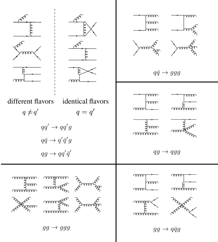
Figure 2: Representative $2\to 3$ Feynman diagrams contributing to $ab\to cX$ to ${\cal{O}}(\alpha_{s}^{3})$.

2.3 $\mathbf{2\to 3}$ real contributions

Figure 2 shows some representative $2\to 3$ Feynman diagrams contributing to $ab\to cX$ to ${\cal{O}}(\alpha_{s}^{3})$. The squared spin-dependent matrix elements in $d$ dimensions, using the HVBM prescription for $\gamma_{5}$ and the Levi-Civita tensor, are too lengthy to be reported here. Again, we have simultaneously calculated the squared matrix elements for the unpolarized case, and we recover the known [26] results in $d$ dimensions. The polarized matrix elements can be checked in $d=4$ dimensions against the expressions in [18], and again we find agreement.

In $d=4-2\varepsilon$ dimensions, as a consequence of using the HVBM scheme with its distinction between four- and $(d-4)$-dimensional subspaces, the squared matrix elements contain scalar products of vectors separately in these subspaces. For instance, while an outgoing unobserved parton with momentum $k$ is massless, $k^{2}=0$, we may encounter its $(d-4)$-dimensional invariant mass, denoted as $\hat{k}^{2}$, in the calculation, which is constructed from the $(d-4)$-dimensional components of $k$. Such terms need to be carefully taken into account in the phase space integrations.

The most economical way of organizing the phase space integration is to work in the rest frame of the two unobserved final-state partons whose momenta $k_{2}$ and $k_{3}$ can then be parameterized as

$$k_{2} = (k_{0},k_{0}\sin\theta_{1}\cos\theta_{2},k_{y},k_{0}\cos\theta_{1},\hat{k})\;\;,$$

$$k_{3} = (k_{0},-k_{0}\sin\theta_{1}\cos\theta_{2},-k_{y},-k_{0}\cos\theta_{1},-\hat{k})\;\;,$$ (15)

and to define the momenta of the other three particles to lie in the $x-z$ plane in the four-dimensional space. In this case the above $\hat{k}^{2}$ is the only invariant arising from the $(d-4)$-dimensional subspace. In Eq. (2.3) $k_{0}=\sqrt{s_{23}}/2$ with $s_{23}=(k_{2}+k_{3})^{2}=s\,v\,(1-w)$, and $k_{y}$ denotes the unspecified $y$ component of $k_{2}$ and $k_{3}$ which can be trivially integrated over since the matrix element does not depend on it. One then has the three-body phase space [11]

$$\Phi_{3}=\frac{s}{(4\pi)^{4}\Gamma(1-2\varepsilon)}\left(\frac{4\pi}{s}\right)^{2\varepsilon}\int_{0}^{1}dvv^{1-2\varepsilon}(1-v)^{-\varepsilon}\int_{0}^{1}dw\left(w(1-w)\right)^{-\varepsilon}$$ (16)

$$\times \int_{0}^{\pi}d\theta_{1}\sin^{1-2\varepsilon}\theta_{1}\int_{0}^{\pi}d\theta_{2}\sin^{-2\varepsilon}\theta_{2}\,\frac{1}{B(\frac{1}{2},-\varepsilon)}\int_{0}^{1}\frac{dx}{\sqrt{1-x}}x^{-(1+\varepsilon)}\>\>,$$

where $x$ is $\hat{k}^{2}$ normalized to its upper limit, $x\equiv 4\hat{k}^{2}/s_{23}\sin^{2}\theta_{1}\sin^{2}\theta_{2}$.

The integrations we do analytically are over $x$ (for those terms in the squared matrix elements that have dependence on $\hat{k}^{2}$) and the angles $\theta_{1}$ and $\theta_{2}$. $v$ and $w$, defined in Eq. (10), become integration variables in the convolution with the parton densities, according to Eqs. (8) and (11). Extensive partial fractioning of the squared matrix elements always leads to the master integral for the angular integrations

$$\!\!\!\!\!\!\!\!\!\!\!\!\int_{0}^{\pi}d\theta_{1}\sin^{1-2\varepsilon}\theta_{1}\int_{0}^{\pi}d\theta_{2}\sin^{-2\varepsilon}\theta_{2}\frac{1}{(1-\cos\theta_{1})^{j}(1-\cos\theta_{1}\cos\chi-\sin\theta_{1}\cos\theta_{2}\sin\chi)^{l}}$$ (17)

$$= 2\pi\frac{\Gamma(1-2\varepsilon)}{\Gamma(1-\varepsilon)}2^{-j-l}\frac{B(1-\varepsilon-j,1-\varepsilon-l)}{\Gamma(1-\varepsilon)}\>{}_{2}F_{1}(j,l,1-\varepsilon;\cos^{2}\frac{\chi}{2})\;\;,$$

where the last line is the result given in Ref. [28]. $B(x,y)$ is the Euler Beta function and ${}_{2}F_{1}(a,b,c;z)$ denotes the hypergeometric function.

The final step in the evaluation of the $2\to 3$ contributions is to extract the poles arising when the invariant mass of the unobserved partons becomes small: $s_{23}\to 0$. According to Eq. (10) or the definition of $s_{23}$ below Eq. (2.3), this is the case for $w\to 1$. The fact that the LO contribution is proportional to $\delta(1-w)$ indicates that the dependence on $w$ is in the sense of a mathematical distribution. At NLO, the integrated matrix elements have terms proportional to $1/(1-w)$ which, after inclusion of the factor $(1-w)^{-\varepsilon}$ from the phase space integral (17), can be expanded as

$$\left(1-w\right)^{-1-\varepsilon}=-\frac{1}{\varepsilon}\delta(1-w)+\frac{1}{(1-w)_{+}}-\varepsilon\left(\frac{\ln(1-w)}{1-w}\right)_{+}+{\cal O}(\varepsilon^{2})\;\;,$$ (18)

making the singularities at $\varepsilon=0$ manifest. Here the “$+$”-distributions are defined in the usual way,

$$\int_{0}^{1}f(w)\left[g(w)\right]_{+}\,dw=\int_{0}^{1}\left[f(w)-f(1)\right]g(w)\,dw\;\;.$$ (19)

2.4 Cancellation of singularities

As mentioned earlier, genuine infrared singularities cancel in the sum of virtual and real contributions, among them all poles proportional to $1/\varepsilon^{2}$ which arise when soft and collinear singularities coalesce. The sum of virtual and real pieces is still singular for $\varepsilon\to 0$ as a result of collinear divergencies. These remaining poles need to be factored into the bare parton distribution functions and fragmentation functions, depending on whether their origin was in the initial or final state.

Figure 3 sketches a typical collinear situation in a $2\to 3$ process. The contribution displayed will require a subtraction of the form $\propto\frac{1}{\varepsilon}\Delta P_{qq}\times\Delta\hat{\sigma}_{qq\to qq}$, where $\Delta P_{qq}$ is the spin-dependent LO $q\to q$ Altarelli-Parisi splitting function [29] and $\Delta\hat{\sigma}_{qq\to qq}$ represents the subsequent polarized LO scattering $qq\to qq$, evaluated in $d$ dimensions. More precisely, the structure of this particular collinear subtraction is

$$-\frac{\alpha_{s}}{\pi}\,\int_{0}^{1}dx\;\Delta H_{qq}(x,\mu_{F})\,\frac{d\Delta\hat{\sigma}_{qq\to qq}(xs,xt,u,\varepsilon)}{dv}\,\delta\left(x\;(s+t)+u\right)\;\;,$$ (20)

where

$$\Delta H_{qq}(z,\mu_{F})\equiv\left(-\frac{1}{\varepsilon}+\gamma_{E}-\ln 4\pi\right)\Delta P_{qq}(z)\left(\frac{s}{\mu_{F}^{2}}\right)^{\varepsilon}+\Delta f_{qq}(z)\;\;.$$ (21)

Here the Euler constant $\gamma_{E}$ and $\ln 4\pi$ are the terms that are commonplace to subtract in order to work in the $\overline{\rm{MS}}$ scheme. $\Delta f_{qq}(z)$ is an additional finite piece in the subtraction that represents the freedom in choosing a factorization prescription and will be discussed below. We see in (21) how the factorization scale $\mu_{F}$ emerges in the subtraction. In general, a process at NLO will require several collinear subtractions, in both the initial and the final states. Depending on which types of partons are collinear, the other splitting functions $\Delta P_{qg}$, $\Delta P_{gq}$, $\Delta P_{gg}$, as well as other $2\to 2$ cross sections, will contribute. In the final-state collinear case, a singularity occurs when the observed parton and an unobserved one become collinear. The subtraction needed here can be easily written down in a form analogous to (21); it will involve the final-state factorization scale $\mu_{F}^{\prime}$. Note that, since we are not considering polarization in the final state, only spin-independent splitting functions appear in the final-state factorization subtraction.

Taking the $\overline{\rm{MS}}$ scheme literally, one would not have any additional finite pieces in the subtraction, beyond those involving $\gamma_{E}$ and $\ln 4\pi$. That is, one would define $(\Delta)f_{ij}(z)=0$ in the functions $(\Delta)H_{ij}$ involved in the various subtractions in the polarized and unpolarized cases. However, there is a well-known [11, 30, 31] subtlety arising in the $q\to q$ splitting in the polarized case that is related to the use of the HVBM scheme. It is a property of the HVBM-scheme definition of $\gamma_{5}$ that it leads to helicity non-conservation at the $qqg$ vertex in $d$ dimensions. This can be seen from the non-vanishing difference of unpolarized and polarized $d$-dimensional LO quark-to-quark splitting functions:

$$\Delta P_{qq}^{4-2\varepsilon}(x)-P_{qq}^{4-2\varepsilon}(x)=4C_{F}\,\varepsilon\,(1-x)\;\;.$$ (22)

Figure 3: Representative collinear contribution to the subprocess $qq\to qqg$ (see text).

A disagreeable consequence of this is a non-zero first moment ($x$-integral) of the flavor non-singlet NLO anomalous dimension for the evolution of spin-dependent quark densities, in conflict with the conservation of flavor non-singlet axial currents [30, 31, 32]. It is therefore advisable – albeit not mandatory in a purely mathematical sense – to slightly deviate from the $\overline{\rm{MS}}$ scheme in the polarized case by choosing [30, 31]

$$\Delta f_{qq}(z)=-4C_{F}(1-z)\;\;.$$ (23)

It is important to point out that the choice of the function $\Delta f_{qq}(z)$ corresponds to the freedom in defining a factorization scheme. Of course, a physical quantity like the pion production cross section must not depend on the convention regarding which finite terms are subtracted from the partonic cross sections along with the collinear poles. Indeed, the parton distributions functions are scheme dependent as well, so that at any given order in $\alpha_{s}$ the scheme dependence cancels in the physical observable. The factorization scheme defined by the choice (23) has also been used in the available sets of spin-dependent NLO $\overline{\mathrm{MS}}$ parton densities, so our definition is consistent with these densities. Since the HVBM “$\gamma_{5}$-effect” mentioned above is to be regarded as an artifact of the prescription and may be removed in a straightforward way by exploiting the conservation of non-singlet axial currents, results of polarized NLO calculations are usually regarded as being “genuinely” in the conventional $\overline{\rm{MS}}$ scheme only with the choice (23). All other possible $\Delta f_{ij}$ are, however, set to zero, as in the usual $\overline{\rm{MS}}$ scheme. Needless to say that in the unpolarized case one has $f_{qq}=f_{qg}=f_{gq}=f_{gg}=0$ in $\overline{\rm{MS}}$.

2.5 Final results

Once we have performed the factorization of collinear singularities, we arrive at the final result for the NLO partonic hard-scattering cross sections. We first of all note that, as mentioned earlier, we have calculated in parallel the NLO corrections for the unpolarized case. We have compared them term-by-term with the known analytical results in the code of [24] and found complete agreement.

Our results for the spin-dependent NLO corrections may for each of the 16 subprocesses be cast into the following form:

$$s\,\frac{d\Delta\hat{\sigma}_{ab}^{c,(1)}(s,v,w,\mu_{R},\mu_{F},\mu_{F}^{\prime})}{dvdw}=\left(\frac{\alpha_{s}(\mu_{R})}{\pi}\right)^{2}\left[\left(A_{0}\delta(1-w)+B_{0}\frac{1}{(1-w)_{+}}+C_{0}\right)\ln\frac{\mu_{F}^{2}}{s}\right.$$

$$+\left(A_{1}\delta(1-w)+B_{1}\frac{1}{(1-w)_{+}}+C_{1}\right)\ln\frac{\mu_{F}^{\prime 2}}{s}+A_{2}\delta(1-w)\ln\frac{\mu_{R}^{2}}{s}$$

$$+A\delta(1-w)+B\frac{1}{(1-w)_{+}}+C+D\left(\frac{\ln(1-w)}{1-w}\right)_{+}+E\ln w+F\ln v$$

$$+G\ln(1-v)+H\ln(1-w)+I\ln(1-vw)+J\ln(1-v+vw)$$

$$\left.+K\frac{\ln w}{1-w}+L\frac{\ln\frac{1-v}{1-vw}}{1-w}+M\frac{\ln(1-v+vw)}{1-w}\right]\>\>\>,$$ (24)

where all coefficients are functions of $v$ and $w$, except those multiplying the distributions $\delta(1-w)$, $1/(1-w)_{+}$, $\left[\ln(1-w)/(1-w)\right]_{+}$ which may be written as functions just of $v$. Terms with distributions are present only for those subprocesses that already contribute at the Born level, see Eq. (2.1).

We finally make a few observations about our results for the polarized case. Consider, for example, the subprocess $q\bar{q}\to q^{\prime}X$ in Eq. (2.1). All Feynman diagrams contributing to this cross section at NLO, virtual as well as real, are annihilation diagrams, meaning that the initial quark and antiquark legs are part of the same fermion line. Independently of the number of gluons attaching to the fermion line, helicity conservation in QCD demands that the annihilation can only occur if the quark and antiquark have opposite helicities. Keeping in mind the definition (5) for the polarized cross section, we are led to the expectation that

$$d\Delta\hat{\sigma}_{q\bar{q}}^{q^{\prime},(1)}\equiv-d\hat{\sigma}_{q\bar{q}}^{q^{\prime},(1)}$$ (25)

should be fulfilled for this process. The only way in which this relation could be broken is if the regularization we adopt in the NLO calculation does not respect helicity conservation. As we discussed earlier, the HVBM prescription for $\gamma_{5}$ indeed has this deficiency. However, as known from [30, 31], the additional finite term $\Delta f_{qq}$ (23) in the factorization subtraction (21) is precisely designed to cure this shortcoming of the HVBM prescription and to restore helicity conservation. This is probably the most tangible reason why the choice Eq. (23) is required from a physical point of view. The implication of this is that our final results for $q\bar{q}\to q^{\prime}X$ should indeed satisfy (25), which we have verified. We can actually go one step further: the channels $q\bar{q}\to gX$ and $q\bar{q}\to qX$ have contributions from annihilation diagrams as well, but also ones from non-annihilation diagrams, for which the $q$ and $\bar{q}$ scatter via $t$-channel gluon exchange. Helicity conservation makes no immediate statement about the non-annihilation diagrams. However, the channels $q\bar{q}^{\prime}\to gX$ and $q\bar{q}^{\prime}\to qX$ are described by the non-annihilation diagrams alone. If we subtract the corresponding cross sections from the ones for $q\bar{q}\to gX$ and $q\bar{q}\to qX$, respectively, we can use helicity conservation again for the remainder. Explicitly, we expect:

$$\left[d\Delta\hat{\sigma}_{q\bar{q}}^{q,(1)}-d\Delta\hat{\sigma}_{q\bar{q}^{\prime}}^{q,(1)}\right]\equiv-\left[d\hat{\sigma}_{q\bar{q}}^{q,(1)}-d\hat{\sigma}_{q\bar{q}^{\prime}}^{q,(1)}\right]\;,$$ (26)

and similarly for an observed gluon. Again we have verified that our final results obey this relation, which we consider a very powerful check on the correctness of our results.

3 Numerical results

In this Section, we present a first numerical application of our analytical results. Instead of presenting a full-fledged phenomenological study of single-inclusive hadron production in polarized $pp$ collisions, which we leave for a future study, we only report the main features of the NLO corrections and describe their impact on the cross sections and the spin asymmetry $A_{LL}^{\pi^{0}}$. Predictions for $A_{LL}^{\pi^{0}}$ are in immediate demand for an extraction of $\Delta g$ at RHIC in the very near future.

For our calculations we assume the same kinematic coverage as in the recent Phenix measurement of the unpolarized cross section at $\sqrt{S}=200\,\mathrm{GeV}$ [16], that is, we consider pion transverse momenta in the range $2\leq p_{T}\leq 13$ GeV and pseudorapidities $|\eta|\leq 0.38$. We also take into account that the pion measurement is at present possible only over half the azimuthal angle.

We will evaluate cross sections and spin asymmetries at both LO and NLO, in order to study the size and importance of the corrections we have calculated. We will always perform the NLO (LO) calculations using NLO (LO) parton distribution functions, fragmentation functions, and the two-loop (one-loop) expression for $\alpha_{s}$. To calculate the NLO (LO) unpolarized pion cross section needed for the denominator of the spin asymmetry $A_{LL}^{\pi^{0}}$ in Eq. (7), we use the CTEQ5M (CTEQ5L) [33] parton distribution functions. In all our calculations we use the pion fragmentation functions of Ref. [34], which provides both a LO and a NLO set. For the polarized cross section, we will mainly use the (NLO/LO) “standard” sets of the spin-dependent GRSV [3] parton distributions (“GRSV-std”). Since we also want to investigate the sensitivity of $A_{LL}^{\pi^{0}}$ to the polarized gluon density $\Delta g$, we use another set of GRSV distributions, for which the gluon is assumed to be particularly large (“GRSV-max”). We note that the value of the strong coupling $\alpha_{s}$ to be used in conjunction with the unpolarized parton distributions differs from that employed in the fits for the polarized sets and the fragmentation functions. Our convention will be to calculate the cross sections always with the strong coupling constant accompanying the parton distributions used.

Figure 4: Unpolarized and polarized $\pi^{0}$ production cross sections in NLO (solid) and LO (dashed) at $\sqrt{S}=200$ GeV. The lower panel shows the ratios of the NLO and LO results in each case.

Figure 4 shows our results for the unpolarized and polarized cross sections at NLO and LO, where we have chosen the scales $\mu_{R}=\mu_{F}=\mu_{F}^{\prime}=p_{T}$. The lower part of the figure displays the “$K$-factor”

$$K=\frac{d(\Delta)\sigma^{\rm NLO}}{d(\Delta)\sigma^{\rm LO}}\;\;.$$ (27)

One can see that in the unpolarized case the corrections are roughly constant and about $50\%$ over the $p_{T}$ region considered. In the polarized case, we find generally smaller corrections which become of similar size as those for the unpolarized case only at the high-$p_{T}$ end. The cross section for $p_{T}$ values smaller than about 2 GeV is outside the domain of perturbative calculations as indicated by rapidly increasing NLO corrections and, therefore, is not considered here.

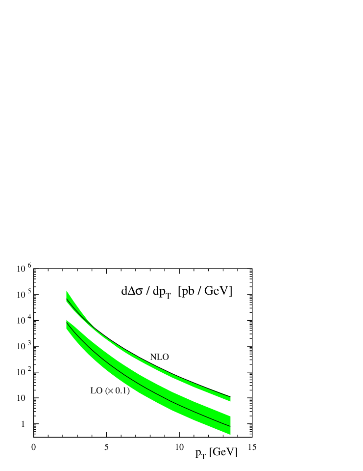
Figure 5: Scale dependence of the polarized cross section for $\pi^{0}$ production at LO and NLO in the range $p_{T}/2\leq\mu_{R}=\mu_{F}=\mu_{F}^{\prime}\leq 2p_{T}$. We have rescaled the LO results by $0.1$ to separate them better from the NLO ones. In each case the solid line corresponds to the choice where all scales are set to $p_{T}$.

As we have mentioned in the Introduction, one reason why NLO corrections are generally important is that they should considerably reduce the dependence of the cross sections on the unphysical factorization and renormalization scales. In this sense, the $K$-factor is actually a quantity of limited significance since it is likely to be rather scale dependent through the presence of the LO cross section in its denominator. The improvement in scale dependence when going from LO to NLO is, therefore, a better measure of the impact of the NLO corrections, and, perhaps, provides also a rough estimate of the relevance of even higher order QCD corrections. Figure 5 shows the scale dependence of the spin-dependent cross section at LO and NLO. In each case the shaded bands indicate the uncertainties from varying the unphysical scales in the range $p_{T}/2\leq\mu_{R}=\mu_{F}=\mu_{F}^{\prime}\leq 2p_{T}$. The solid lines are for the choice where all scales are set to $p_{T}$. One can see that the scale dependence indeed becomes much smaller at NLO.

Finally, we consider the spin asymmetry which is the main quantity of interest here. Figure 6 shows $A_{LL}^{\pi^{0}}$, calculated at NLO (solid lines) for the “standard” set of GRSV parton distributions, and for the one with “maximal” gluon polarization [3]. We have again chosen all scales to be $p_{T}$. For comparison, we also show the LO result for the GRSV “standard” set (dashed line). As expected from the larger $K$ factor for the unpolarized cross section shown in Fig. 4, the asymmetry is somewhat smaller at NLO than at LO, showing that inclusion of NLO QCD corrections is rather important for the analysis of the data in terms of $\Delta g$.

Figure 6: Spin asymmetry for $\pi^{0}$ production, using the “standard” set of GRSV [3] and the one with “maximal” gluon polarization. The dashed line shows the asymmetry at LO for the GRSV “standard” set. The “error bars” indicate the expected statistical accuracy targeted for the upcoming run of RHIC (see text).

We also conclude from the figure that there are excellent prospects for determining $\Delta g(x)$ from $A_{LL}^{\pi^{0}}$ measurements at RHIC: the asymmetries found for the two different sets of polarized parton densities, which mainly differ in the gluon density, show marked differences, much larger than the expected statistical errors in the experiment, indicated in the figure. The latter may be estimated by the formula

$$\delta A_{LL}^{\pi}=\frac{1}{P^{2}\sqrt{{\cal L}\sigma_{\rm bin}}}\;,$$ (28)

where $P$ is the polarization of one beam, ${\cal L}$ the integrated luminosity of the collisions, and $\sigma_{\rm bin}$ the unpolarized cross section integrated over the $p_{T}$-bin for which the error is to be determined. We have used the very moderate values $P=0.4$ and ${\cal L}=7$/pb, which are targets for the coming run. As mentioned above, we also take into account that at present with the Phenix experiment a pion measurement is possible only over half the azimuthal angle.

4 Conclusions

We have presented in this paper the complete NLO QCD corrections for the partonic hard-scattering cross sections relevant for the spin asymmetry $A_{LL}^{\pi}$ for high-$p_{T}$ pion production in hadron-hadron collisions. This asymmetry is a promising tool to determine the spin-dependent gluon density in the nucleon and will be measured in the coming run with polarized protons at RHIC. Our calculation is based on a largely analytical evaluation of the NLO partonic cross sections.

We found that the NLO corrections to the polarized cross section are somewhat smaller for RHIC than those in the unpolarized case. The polarized cross section shows a significant reduction of scale dependence when going from LO to NLO. Upcoming RHIC data should be able to provide first information on $\Delta g$ even for rather moderate integrated luminosities.

Note added:

While nearing completion of our work, we learned that D. de Florian has performed [35] the same calculation, using the “Monte-Carlo” method outlined in Sec. 2. This provides an extremely welcome opportunity for comparing the results. Early comparisons show very good agreement of the numerical results.

References

-
[1]
European Muon Collaboration (EMC), J. Ashman et al.,
Phys. Lett. B206, 364 (1988);
Nucl. Phys. B328, 1 (1989);
for a recent review of the data on polarized deep-inelastic scattering, see: E. Hughes and R. Voss, Annu. Rev. Nucl. Part. Sci. 49, 303 (1999). -
[2]
J.C. Collins and D. Soper, Nucl. Phys. B194, 445 (1982);
A. Manohar, Phys. Rev. Lett. 65, 2511 (1990);
R.L. Jaffe, Phys. Lett. B365, 359 (1996). - [3] M. Glück, E. Reya, M. Stratmann, and W. Vogelsang, Phys. Rev. D63, 094005 (2001).
-
[4]
M. Glück, E. Reya, M. Stratmann, and
W. Vogelsang, Phys. Rev. D53, 4775 (1996);
G. Altarelli, R.D. Ball, S. Forte, and G. Ridolfi, Nucl. Phys. B496, 337 (1997); Acta Phys. Polon. B29, 1145 (1998);
T. Gehrmann and W.J. Stirling, Phys. Rev. D53, 6100 (1996);
SM Collaboration (SMC), D. Adams et al., Phys. Rev. D56, 5330 (1997); SMC, B. Adeva et al., Phys. Rev. D58, 112002 (1998);
D. de Florian, O.A. Sampayo, and R. Sassot, Phys. Rev. D57, 5803 (1998);
D. de Florian and R. Sassot, Phys. Rev. D62, 094025 (2000);
Asymmetry Analysis Collaboration, Y. Goto et al., Phys. Rev. D62, 034017 (2000);
E. Leader, A.V. Sidorov, and D. Stamenov, Eur. Phys. J. C23, 479 (2002);
J. Blümlein and H. Böttcher, Nucl. Phys. B636, 225 (2002). - [5] COMPASS Collaboration, G. Baum et al., CERN/SPSLC 96-14 (1996).
- [6] HERMES Collaboration, “The HERMES Physics Program & Plans for 2001-2006”, DESY-PRC (2000).
- [7] See http://www.bnl.gov/eic for information concerning the EIC project, including the EIC Whitepaper.
- [8] See, for example: G. Bunce, N. Saito, J. Soffer, and W. Vogelsang, Annu. Rev. Nucl. Part. Sci. 50, 525 (2000).
-
[9]
S.B. Libby and G. Sterman, Phys. Rev. D18, 3252 (1978);
R.K. Ellis, H. Georgi, M. Machacek, H.D. Politzer, and G.G. Ross, Phys. Lett. 78B, 281 (1978); Nucl. Phys. B152, 285 (1979);
D. Amati, R. Petronzio, and G. Veneziano, Nucl. Phys. B140, 54 (1980); Nucl. Phys. B146, 29 (1978);
G. Curci, W. Furmanski, and R. Petronzio, Nucl. Phys. B175, 27 (1980);
J.C. Collins, D.E. Soper, and G. Sterman, Phys. Lett. B134, 263 (1984); Nucl. Phys. B261, 104 (1985);
J.C. Collins, Nucl. Phys. B394, 169 (1993). -
[10]
A.P. Contogouris, B. Kamal, Z. Merebashvili, and
F.V. Tkachov, Phys. Lett. B304, 329 (1993);
Phys. Rev. D48, 4092 (1993);
A.P. Contogouris and Z. Merebashvili, Phys. Rev. D55, 2718 (1997). - [11] L.E. Gordon and W. Vogelsang, Phys. Rev. D48, 3136 (1993); Phys. Rev. D49, 170 (1994).
- [12] S. Frixione and W. Vogelsang, Nucl. Phys. B568, 60 (2000).
- [13] D. de Florian, S. Frixione, A. Signer, and W. Vogelsang, Nucl. Phys. B539, 455 (1999).
- [14] I. Bojak and M. Stratmann, hep-ph/0112276.
-
[15]
P.G. Ratcliffe, Nucl. Phys. B223, 45 (1983);
A. Weber, Nucl. Phys. B382, 63 (1992);
B. Kamal, Phys. Rev. D57, 666 (1998);
T. Gehrmann, Nucl. Phys. B534, 21 (1998). - [16] H. Torii, PHENIX Collaboration, talk presented at the “XVI International Conference on Ultrarelativistic Nucleus-Nucleus Collisions (Quark Matter 2002)”, Nantes, France, July 2002.
- [17] See, for example: J. Babcock, E. Monsay, and D. Sivers, Phys. Rev. Lett. 40, 1161 (1978); Phys. Rev. D19, 1483 (1979).
- [18] R. Gastmans and T.T. Wu, “The ubiquitous photon”, Oxford Science Publications, Clarendon Press, Oxford, 1990.
- [19] G. ’t Hooft and M. Veltman, Nucl. Phys. B44, 189 (1972); P. Breitenlohner and D. Maison, Commun. Math. Phys. 52, 11 (1977).
- [20] M. Jamin and M.E. Lautenbacher, Comput. Phys. Commun. 74, 265 (1993).
-
[21]
W.T. Giele and E.W.N. Glover, Phys. Rev. D46, 1980 (1992);
W.T. Giele, E.W.N. Glover, and D.A. Kosower, Nucl. Phys. B403, 633 (1993);
S. Frixione, Z. Kunszt, and A. Signer, Nucl. Phys. B467, 399 (1996);
S. Catani and M. Seymour, Nucl. Phys. B485, 291 (1997), Erratum B510, 503 (1998);
S. Frixione, Nucl. Phys. B507, 295 (1997). - [22] Z. Kunszt and D. Soper, Phys. Rev. D46, 192 (1992).
- [23] M. Stratmann and W. Vogelsang, Phys. Rev. D64, 114007 (2001).
- [24] F. Aversa, P. Chiappetta, M. Greco, and J.-Ph. Guillet, Nucl. Phys. B327, 105 (1989).
- [25] M.A. Nowak, M. Praszalowicz, and W. Slominski, Annals Phys. 166, 443 (1986).
- [26] R.K. Ellis and J.C. Sexton, Nucl. Phys. B269, 445 (1986).
- [27] Z. Kunszt, A. Signer, and Z. Trocsanyi, Nucl. Phys. B411, 397 (1994).
- [28] W.L. van Neerven, Nucl. Phys. B268, 453 (1986).
- [29] G. Altarelli and G. Parisi, Nucl. Phys. B126, 298 (1977).
- [30] R. Mertig and W.L. van Neerven, Z. Phys. C70, 637 (1996).
- [31] W. Vogelsang, Phys. Rev. D54, 2023 (1996); Nucl. Phys. B475, 47 (1996).
- [32] M. Stratmann, W. Vogelsang, and A. Weber, Phys. Rev. D53, 138 (1996).
- [33] CTEQ Collaboration, H.-L. Lai et al., Eur. Phys. J. C12, 375 (2000).
- [34] B.A. Kniehl, G. Kramer, and B. Pötter, Nucl. Phys. B582, 514 (2000).
- [35] D. de Florian, hep-ph/0210442.