PCCF-RI-02-07

ADP-02-94/T532

Direct $CP$ Violation in $B\rightarrow\pi^{+}\pi^{-}\pi$
Determination of $\alpha$ without discrete ambiguity

O. Leitner^1,2, X.-H. Guo¹, A.W. Thomas^1
1 Department of Physics and Mathematical Physics, and

Special Research Center for the Subatomic Structure of Matter,

University of Adelaide, Adelaide 5005, Australia

² Laboratoire de Physique Corpusculaire, Université Blaise Pascal,

CNRS/IN2P3, 24 avenue des Landais, 63177 Aubière Cedex, France

Direct $CP$ violation in the hadronic decays $\bar{B}^{0}\rightarrow\pi^{+}\pi^{-}\pi^{0}$ is investigated near the peak of the $\rho^{0}$ taking into account the effect of $\rho-\omega$ mixing. Branching ratios for processes $B^{\pm,0}\rightarrow\rho^{\pm,0}\pi^{\pm,0}$ and $B^{-}\rightarrow\omega\pi^{-}$ are calculated as well. We find that the $CP$ violating asymmetry is strongly dependent on the CKM matrix elements. For a fixed $N_{c}^{eff}$, the $CP$ violating asymmetry, $a_{CP}$, has a maximum of order $-40\%$ to $-70\%$ for $\bar{B}^{0}\rightarrow\rho^{0}(\omega)\pi^{0}$ when the invariant mass of the $\pi^{+}\pi^{-}$ pair is in the vicinity of the $\omega$ resonance. The sensitivity of the asymmetry to $N_{c}^{eff}$ is small in that case. Moreover, we find that in the range of $N_{c}^{eff}$ which is allowed by the most recent experimental branching ratios from the BABAR, BELLE and CLEO Collaborations, the sign of $\sin\delta$ is always positive. Thus, a measurement of direct $CP$ violation in decays $\bar{B}^{0}\rightarrow\pi^{+}\pi^{-}\pi^{0}$ would remove the mod$(\pi)$ ambiguity in the determination of the $CP$ violating phase angle $\alpha$.

PACS Numbers: 11.30.Er, 12.39.-x, 13.25.Hw.

1 Introduction

In the Standard Model, $CP$ violating phenomena arise from a non-zero weak phase angle in a complex matrix allowing flavour violation in the weak interaction: the Cabbibo-Kobayashi-Maskawa (CKM) matrix. Although the source of $CP$ violation has not been well understood up to now, physicists are striving to increase their knowledge of the mechanism. Many theoretical studies [1, 2] (within and beyond the Standard Model) and experimental investigations have been conducted since the discovery of $CP$ violation in neutral Kaon decays (1964). According to theoretical predictions, large $CP$ violating effects may be expected in $B$ meson decays. In the past few years, several facilities have started to collect events on $B$ decays and most of them refer to branching ratios. Generally, the main theoretical uncertainties apart from the CKM matrix elements are the hadronic matrix elements, where non-factorizable effects are involved. As regards hadronic matrix elements and non-factorizable effects, a new QCD factorization approach [3] has been proposed. This QCD factorization approach includes all radiative diagrams (gluon exchange) but will not be the subject of this paper. For the CKM matrix elements, uncertainties in the parameters $\rho$ and $\eta$ have been reduced and this allows us to predict $CP$ violating asymmetry in $B$ decays more accurately than before. This will give us an excellent test for the Standard Model and may lead to suggestions of new physics.
Direct $CP$ violating asymmetries in $B$ decays occur through the interference of at least two amplitudes with different weak phase $\phi$ and strong phase $\delta$. In order to extract the weak phase (which is determined by the CKM matrix elements), one must know the strong phase $\delta$ and this is usually not well determined. In addition, in order to have a large signal, we have to appeal to some phenomenological mechanism to obtain a large $\delta$. The charge symmetry violating mixing between $\rho^{0}$ and $\omega$ can be extremely important in this regard. In particular, it can lead to a large $CP$ violation in $B$ decay such as $\bar{B}^{0}\rightarrow\rho^{0}(\omega)\pi^{0}\rightarrow\pi^{+}\pi^{-}\pi^{0}$, because the strong phase passes through $90^{o}$ at the $\omega$ resonance [4, 5, 6].
We have collected all the recent data for $b$ to $d$ transitions, but we shall focus on the CLEO, BABAR and BELLE branching ratio results. We also shall use the latest values for CKM parameters, $A,\lambda,\rho$, and $\eta$. The aim of the present work is to constrain the $CP$ violating calculation in $\bar{B}^{0}\rightarrow\rho^{0}(\omega)\pi^{0}\rightarrow\pi^{+}\pi^{-}\pi^{0}$, including $\rho-\omega$ mixing and using the most recent experimental data for the branching ratios for $B\rightarrow\rho\pi$ decays. In order to extract the strong phase $\delta$, we use the naive factorization approach, in which the hadronic matrix elements of operators are saturated by vacuum intermediate states. Moreover, we approximate non-factorizable effects by introducing an effective number of colours, $N_{c}^{eff}$.
In this paper, we investigate five phenomenological models with different weak form factors and determine the $CP$ violating asymmetry for $\bar{B}^{0}\rightarrow\rho^{0}(\omega)\pi^{0}\rightarrow\pi^{+}\pi^{-}\pi^{0}$ in these models. We select models which are consistent with all the latest data and determine the allowed range for $N_{c}^{eff}$ ($1.09(1.11)<N_{c}^{eff}<1.68(1.80)$). Then, we study the sign of $\sin\delta$ in this range of $N_{c}^{eff}$ in all these models. We also discuss the model dependence of our results in detail.
This paper is structured as follows. In Section 2, we introduce the effective Hamiltonian based on the Operator Product Expansion (OPE) including Wilson coefficients. We also present the formalism of $\rho-\omega$ mixing and its application to the $CP$ violating asymmetry in decay processes. In Section 3, the CKM matrix and the relevant form factors are discussed. In Section 4, we present numerical results for the $CP$ violating asymmetry in $\bar{B}^{0}\rightarrow\pi^{+}\pi^{-}\pi^{0}$ which is followed by discussion of these results. In Section 5, branching ratios for decays such as $B^{\pm,0}\rightarrow\rho^{\pm,0}\pi^{\pm,0}$ and $B^{-}\rightarrow\omega\pi^{-}$ are investigated. From the CLEO, BABAR and BELLE experimental data for these branching ratios, we extract the range of $N_{c}^{eff}$ allowed in these processes and the results are also discussed. In the final section, we summarize our results. Comments on form factors, CKM matrix parameter values, $\rho,\eta$, and conclusions are also given in this section.

2 $\boldsymbol{CP}$ violation in $\boldsymbol{\bar{B}^{0}\rightarrow\rho^{0}\pi^{0}\rightarrow\pi^{+}\pi^{-}\pi^{0}}$

2.1 Effective theory

In any phenomenological treatment of the weak decays of hadrons, the starting point is the weak effective Hamiltonian at low energy [7] from which, the decay amplitude can be expressed as follows,

$$A(B\rightarrow PV)=\frac{G_{F}}{\sqrt{2}}\biggl{[}V_{ub}V_{ud}^{\ast}\bigl{(}C_{1}\langle PV|O_{1}^{u}|B\rangle+C_{2}\langle PV|O_{2}^{u}|B\rangle\bigr{)}\\ -V_{tb}V_{td}^{\ast}\sum_{i=3}^{10}C_{i}\langle PV|O_{i}|B\rangle\biggr{]}+h.c.\ ,$$ (1)

where $\langle PV|O_{i}|B\rangle$ are the hadronic matrix elements. They describe the transition between initial and final states with the operator renormalized at scale $\mu$ and include, up to now, the main uncertainties in the calculation since they involve non-perturbative effects. $G_{F}$ is the Fermi constant, $V_{CKM}$ is the CKM matrix element, $C_{i}(\mu)$ are the Wilson coefficients, $O_{i}(\mu)$ are the operators from OPE [8]. The operators $O_{i}$, the local operators which govern weak decays can be written as,

$$O_{1}^{u} =\bar{q}_{\alpha}\gamma_{\mu}(1-\gamma{{}_{5}})u_{\beta}\bar{u}_{\beta}\gamma^{\mu}(1-\gamma{{}_{5}})b_{\alpha}\ , O_{2}^{u} =\bar{q}\gamma_{\mu}(1-\gamma{{}_{5}})u\bar{u}\gamma^{\mu}(1-\gamma{{}_{5}})b\ ,$$

$$O_{3} =\bar{q}\gamma_{\mu}(1-\gamma{{}_{5}})b\sum_{q\prime}\bar{q}^{\prime}\gamma^{\mu}(1-\gamma{{}_{5}})q^{\prime}\ , O_{4} =\bar{q}_{\alpha}\gamma_{\mu}(1-\gamma{{}_{5}})b_{\beta}\sum_{q\prime}\bar{q}^{\prime}_{\beta}\gamma^{\mu}(1-\gamma{{}_{5}})q^{\prime}_{\alpha}\ ,$$

$$O_{5} =\bar{q}\gamma_{\mu}(1-\gamma{{}_{5}})b\sum_{q^{\prime}}\bar{q}^{\prime}\gamma^{\mu}(1+\gamma{{}_{5}})q^{\prime}\ , O_{6} =\bar{q}_{\alpha}\gamma_{\mu}(1-\gamma{{}_{5}})b_{\beta}\sum_{q^{\prime}}\bar{q}^{\prime}_{\beta}\gamma^{\mu}(1+\gamma{{}_{5}})q^{\prime}_{\alpha}\ ,$$

$$O_{7} =\frac{3}{2}\bar{q}\gamma_{\mu}(1-\gamma{{}_{5}})b\sum_{q^{\prime}}e_{q^{\prime}}\bar{q}^{\prime}\gamma^{\mu}(1+\gamma{{}_{5}})q^{\prime}\ , O_{8} =\frac{3}{2}\bar{q}_{\alpha}\gamma_{\mu}(1-\gamma{{}_{5}})b_{\beta}\sum_{q^{\prime}}e_{q^{\prime}}\bar{q}^{\prime}_{\beta}\gamma^{\mu}(1+\gamma{{}_{5}})q^{\prime}_{\alpha}\ ,$$

$$O_{9} =\frac{3}{2}\bar{q}\gamma_{\mu}(1-\gamma{{}_{5}})b\sum_{q^{\prime}}e_{q^{\prime}}\bar{q}^{\prime}\gamma^{\mu}(1-\gamma{{}_{5}})q^{\prime}\ , O_{10} =\frac{3}{2}\bar{q}_{\alpha}\gamma_{\mu}(1-\gamma{{}_{5}})b_{\beta}\sum_{q^{\prime}}e_{q^{\prime}}\bar{q}^{\prime}_{\beta}\gamma^{\mu}(1-\gamma{{}_{5}})q^{\prime}_{\alpha}\ ,$$ (2)

where $q^{\prime}=u,d,s,c$ and $e_{q^{\prime}}$ denotes its electric charge. As regards the Wilson coefficients [9, 10, 11, 12], they represent the physical contributions from scales higher than $\mu$. Since QCD has the property of asymptotic freedom, they can be calculated in perturbation theory. Usually, the scale $\mu$ is chosen to be of order $O(m_{b})$ for $B$ decays and Wilson coefficients have been calculated to the next-to-leading order (NLO). For more details see Ref. [13].

2.2 $\boldsymbol{\rho-\omega}$ Mixing

Let $A$ be the amplitude for the decay $B\rightarrow\rho^{0}\pi\rightarrow\pi^{+}\pi^{-}\pi$ then one has,

$$A=\langle\pi\pi^{-}\pi^{+}|H^{T}|B\rangle+\langle\pi\pi^{-}\pi^{+}|H^{P}|B\rangle\ ,$$ (3)

with $H^{T}$ and $H^{P}$ being the Hamiltonians for the tree and penguin operators. We can define the relative magnitude and phases between these two contributions as follows,

$$A =\langle\pi\pi^{-}\pi^{+}|H^{T}|B\rangle[1+re^{i\delta}e^{i\phi}]\ ,$$

$$\bar{A} =\langle\bar{\pi}\pi^{+}\pi^{-}|H^{T}|\bar{B}\rangle[1+re^{i\delta}e^{-i\phi}]\ ,$$ (4)

where $\delta$ and $\phi$ are the strong and weak phases, respectively. The phase $\phi$ arises from the appropriate combination of CKM matrix elements, and, assuming top quark dominance, $\phi={\rm arg}[(V_{tb}V_{td}^{\star})/(V_{ub}V_{ud}^{\star})]$. As a result, $\sin\phi$ is equal to $\sin\alpha$, with $\alpha$ defined in the standard way [14]. The parameter, $r$, is the absolute value of the ratio of tree and penguin amplitudes:

$$r\equiv\left|\frac{\langle\rho^{0}\pi|H^{P}|B\rangle}{\langle\rho^{0}\pi|H^{T}|B\rangle}\right|.$$ (5)

In order to obtain a large signal for direct $CP$ violation, we need some mechanism to make both $\sin\delta$ and $r$ large. We stress that $\rho-\omega$ mixing [15] has the dual advantages that the strong phase difference is large (passing through $90^{o}$ at the $\omega$ resonance) and well known [5, 6]. With this mechanism, to first order in isospin violation, we have the following results when the invariant mass of $\pi^{+}\pi^{-}$ is near the $\omega$ resonance mass,

$$\langle\pi\pi^{-}\pi^{+}|H^{T}|B\rangle =\frac{g_{\rho}}{s_{\rho}s_{\omega}}\tilde{\Pi}_{\rho\omega}t_{\omega}+\frac{g_{\rho}}{s_{\rho}}t_{\rho}\ ,$$

$$\langle\pi\pi^{-}\pi^{+}|H^{P}|B\rangle =\frac{g_{\rho}}{s_{\rho}s_{\omega}}\tilde{\Pi}_{\rho\omega}p_{\omega}+\frac{g_{\rho}}{s_{\rho}}p_{\rho}\ .$$ (6)

Here $t_{V}(V=\rho\;{\rm or}\;\omega)$ is the tree amplitude and $p_{V}$ the penguin amplitude for producing a vector meson, V, $g_{\rho}$ is the coupling for $\rho^{0}\rightarrow\pi^{+}\pi^{-}$, $\tilde{\Pi}_{\rho\omega}$ is the effective $\rho-\omega$ mixing amplitude, and $s_{V}$ is from the inverse propagator of the vector meson V,

$$s_{V}=s-m_{V}^{2}+im_{V}\Gamma_{V}\ ,$$ (7)

with $\sqrt{s}$ being the invariant mass of the $\pi^{+}\pi^{-}$ pair. We stress that the direct coupling $\omega\rightarrow\pi^{+}\pi^{-}$ is effectively absorbed into $\tilde{\Pi}_{\rho\omega}$ [16], leading to the explicit $s$ dependence of $\tilde{\Pi}_{\rho\omega}$. Making the expansion $\tilde{\Pi}_{\rho\omega}(s)=\tilde{\Pi}_{\rho\omega}(m_{\omega}^{2})+(s-m_{w}^{2})\tilde{\Pi}_{\rho\omega}^{\prime}(m_{\omega}^{2})$, the $\rho-\omega$ mixing parameters were determined in the fit of Gardner and O’Connell [17]: $\Re e\;\tilde{\Pi}_{\rho\omega}(m_{\omega}^{2})=-3500\pm 300\;{\rm MeV}^{2},\;\;\;\Im m\;\tilde{\Pi}_{\rho\omega}(m_{\omega}^{2})=-300\pm 300\;{\rm MeV}^{2}$ and $\tilde{\Pi}_{\rho\omega}^{\prime}(m_{\omega}^{2})=0.03\pm 0.04$. In practice, the effect of the derivative term is negligible. From Eqs. (3, 2.2, 2.2) one has,

$$re^{i\delta}e^{i\phi}=\frac{\tilde{\Pi}_{\rho\omega}p_{\omega}+s_{\omega}p_{\rho}}{\tilde{\Pi}_{\rho\omega}t_{\omega}+s_{\omega}t_{\rho}}\ .$$ (8)

Defining,

$$\frac{p_{\omega}}{t_{\rho}}\equiv r^{\prime}e^{i(\delta_{q}+\phi)}\ ,\;\;\;\;\frac{t_{\omega}}{t_{\rho}}\equiv\alpha e^{i\delta_{\alpha}}\ ,\;\;\;\;\frac{p_{\rho}}{p_{\omega}}\equiv\beta e^{i\delta_{\beta}}\ ,$$ (9)

where $\delta_{\alpha},\delta_{\beta}$, and $\delta_{q}$ are strong phases (absorptive part). Substituting Eq. (9) into Eq. (8), one finds,

$$re^{i\delta}=r^{\prime}e^{i\delta_{q}}\frac{\tilde{\Pi}_{\rho\omega}+\beta e^{i\delta_{\beta}}s_{\omega}}{s_{\omega}+\tilde{\Pi}_{\rho\omega}\alpha e^{i\delta_{\alpha}}}\ .$$ (10)

$\alpha e^{i\delta_{\alpha}}$, $\beta e^{i\delta_{\beta}}$, and $r^{\prime}e^{i\delta_{q}}$ will be calculated later. In order to get the $CP$ violating asymmetry $a_{CP}$, $\sin\phi$ and $\cos\phi$ are needed, where $\phi$ is determined by the CKM matrix elements. In the Wolfenstein parametrization, the weak phase comes from $[V_{tb}V^{\star}_{td}/V_{ub}V^{\star}_{ud}]$ and one has for the decay $B\rightarrow\rho(\omega)\pi$,

$$\sin\phi =\frac{\eta}{\sqrt{[\rho(1-\rho)-\eta^{2}]^{2}+\eta^{2}}}\ ,$$

$$\cos\phi =\frac{\rho(1-\rho)-\eta^{2}}{\sqrt{[\rho(1-\rho)-\eta^{2}]^{2}+\eta^{2}}}\ .$$ (11)

The values used for $\rho$ and $\eta$ will be discussed in Section 3.1. With the decay amplitude given in Eq. (1), we are ready to evaluate the matrix elements for $B^{\pm,0}\rightarrow\rho^{0}(\omega)\pi^{\pm,0}$. In the factorization approximation [18], either $\rho^{0}(\omega)$ or $\pi^{\pm,0}$ is generated by one current which has the appropriate quantum numbers in the Hamiltonian. For these decay processes, two kinds of matrix element products are involved after factorization; schematically (i.e. omitting Dirac matrices and colour labels) one has $\langle\rho^{0}(\omega)|(\bar{u}u)|0\rangle\langle\pi^{\pm,0}|(\bar{u}b)|B^{\pm,0}\rangle$ and $\langle\pi^{\pm,0}|(\bar{q}_{1}q_{2})|0\rangle\langle\rho^{0}(\omega)|(\bar{u}b)|B^{\pm,0}\rangle$ with $q_{i}(i=1,2)=u,d$. We will calculate them in some phenomenological quark models.
The matrix elements for $B\rightarrow X$ and $B\rightarrow X^{\star}$ (where X and $X^{\star}$ denote pseudoscalar and vector mesons, respectively) can be decomposed as follows [19],

$$\langle X|J_{\mu}|B\rangle=\left(p_{B}+p_{X}-\frac{m_{B}^{2}-m_{X}^{2}}{k^{2}}k\right)_{\mu}F_{1}(k^{2})+\frac{m_{B}^{2}-m_{X}^{2}}{k^{2}}k_{\mu}F_{0}(k^{2})\ ,$$ (12)

and

$$\langle X^{\star}|J_{\mu}|B\rangle=\frac{2}{m_{B}+m_{X^{\star}}}\epsilon_{\mu\nu\rho\sigma}\epsilon^{\star\nu}p_{B}^{\rho}p_{X^{\star}}^{\sigma}V(k^{2})+i\Biggl{\{}\epsilon_{\mu}^{\star}(m_{B}+m_{X^{\star}})A_{1}(k^{2})\\ -\frac{\epsilon^{\star}\cdot k}{m_{B}+m_{X^{\star}}}(P_{B}+P_{X^{\star}})_{\mu}A_{2}(k^{2})-\frac{\epsilon^{\star}\cdot k}{k^{2}}2m_{X^{\star}}\cdot k_{\mu}A_{3}(k^{2})\Biggr{\}}\\ +i\frac{\epsilon^{\star}\cdot k}{k^{2}}2m_{X^{\star}}\cdot k_{\mu}A_{0}(k^{2})\ ,$$ (13)

where $J_{\mu}(=\bar{q}\gamma^{\mu}(1-\gamma_{5})b)$ is the weak current with $q=u,d$, $k=p_{B}-p_{X(X^{\star})}$, and $\epsilon_{\mu}$ is the polarization vector of $X^{\star}$. $F_{0}$ and $F_{1}$ are the form factors related to the transition $0^{-}\rightarrow 0^{-}$ and $A_{0},A_{1},A_{2},A_{3}$, and $V$ are the form factors which describe the transition $0^{-}\rightarrow 1^{-}$. Finally, in order to cancel the poles at $q^{2}=0$, the form factors must respect the constraints:

$$F_{1}(0)=F_{0}(0),\;\;A_{3}(0)=A_{0}(0)\ .$$ (14)

They also satisfy the following relations:

$$A_{3}(k^{2})=\frac{m_{B}+m_{X^{\star}}}{2m_{X^{\star}}}A_{1}(k^{2})-\frac{m_{B}-m_{X^{\star}}}{2m_{X^{\star}}}A_{2}(k^{2})\ .$$ (15)

By using the decomposition in Eqs. (12, 13), one obtains the following tree operator contribution for the process $\bar{B}^{0}\rightarrow\rho^{0}(\omega)\pi^{0}$:

$$t_{\rho}=m_{B}|\vec{p}_{\rho}|\biggl{[}(C_{1}^{\prime}+\frac{1}{N_{c}^{eff}}C_{2}^{\prime})\biggr{]}\biggl{(}f_{\rho}F_{1}(m_{\rho}^{2})+f_{\pi}A_{0}(m_{\pi}^{2})\biggr{)}\ ,$$ (16)

where $f_{\rho}$ and $f_{\pi}$ are the decay constants of $\rho$ and $\pi$, respectively, and $C_{i}^{\prime}$ are the Wilson coefficients with values listed in Table 1. We find $t_{\omega}\neq t_{\rho}$, so that

$$\alpha e^{i\delta_{\alpha}}=\frac{-f_{\rho}F_{1}(m_{\rho}^{2})+f_{\pi}A_{0}(m_{\pi}^{2})}{f_{\rho}F_{1}(m_{\rho}^{2})+f_{\pi}A_{0}(m_{\pi}^{2})}\ .$$ (17)

After calculating the penguin operator contributions, one has,

$$r^{\prime}e^{i\delta_{q}}=-\frac{p_{\omega}}{(C_{1}^{\prime}+\frac{1}{N_{c}^{eff}}C_{2}^{\prime})\bigl{(}f_{\rho}F_{1}(m_{\rho}^{2})+f_{\pi}A_{0}(m_{\pi}^{2})\bigr{)}}\left|\frac{V_{tb}V_{td}^{\star}}{V_{ub}V_{ud}^{\star}}\right|\ ,$$ (18)

and

$$\beta e^{i\delta_{\beta}}=\frac{m_{B}|\vec{p}_{\rho}|}{p_{\omega}}\Bigg{\{}-(C_{4}^{\prime}+\frac{1}{N_{c}^{eff}}C_{3}^{\prime})[f_{\rho}F_{1}(m_{\rho}^{2})+f_{\pi}A_{0}(m_{\pi}^{2})]\\ \hskip 50.00008pt-\frac{3}{2}[(C_{7}^{\prime}+\frac{1}{N_{c}^{eff}}C_{8}^{\prime})-(C_{9}^{\prime}+\frac{1}{N_{c}^{eff}}C_{10}^{\prime})]f_{\pi}A_{0}(m_{\pi}^{2})\\ \hskip 50.00008pt+\frac{3}{2}[(C_{7}^{\prime}+\frac{1}{N_{c}^{eff}}C_{8}^{\prime})+(C_{9}^{\prime}+\frac{1}{N_{c}^{eff}}C_{10}^{\prime})]f_{\rho}F_{1}(m_{\rho}^{2})\\ +[(C_{6}^{\prime}+\frac{1}{N_{c}^{eff}}C_{5}^{\prime})-\frac{1}{2}(C_{8}^{\prime}+\frac{1}{N_{c}^{eff}}C_{7}^{\prime})]\left[\frac{2m_{\pi}^{2}f_{\pi}A_{0}(m_{\pi}^{2})}{(m_{d}+m_{d})(m_{b}+m_{d})}\right]\\ +\frac{1}{2}(C_{10}^{\prime}+\frac{1}{N_{c}^{eff}}C_{9}^{\prime})[f_{\rho}F_{1}(m_{\rho}^{2})+f_{\pi}A_{0}(m_{\pi}^{2})]\Bigg{\}}\ ,$$ (19)

where $\vec{p}_{\rho}$ is the c.m. momentum of the decay process. In Eqs. (18, 19), $p_{\omega}$ is written as,

$$p_{\omega}=m_{B}|\vec{p}_{\rho}|\Bigg{\{}-2\left[(C_{3}^{\prime}+\frac{1}{N_{c}^{eff}}C_{4}^{\prime})+(C_{5}^{\prime}+\frac{1}{N_{c}^{eff}}C_{6}^{\prime})\right]f_{\rho}F_{1}(m_{\rho}^{2})\\ \hskip 50.00008pt-\frac{1}{2}\left[(C_{7}^{\prime}+\frac{1}{N_{c}^{eff}}C_{8}^{\prime})+(C_{9}^{\prime}+\frac{1}{N_{c}^{eff}}C_{10}^{\prime})\right]f_{\rho}F_{1}(m_{\rho}^{2})\\ -\left[\frac{1}{2}(C_{8}^{\prime}+\frac{1}{N_{c}^{eff}}C_{7}^{\prime})-(C_{6}^{\prime}+\frac{1}{N_{c}^{eff}}C_{5}^{\prime})\right]\left[\frac{2m_{\pi}^{2}f_{\pi}A_{0}(m_{\pi}^{2})}{(m_{d}+m_{d})(m_{b}+m_{d})}\right]\\ \hskip 95.00014pt-(C_{4}^{\prime}+\frac{1}{N_{c}^{eff}}C_{3}^{\prime})\left[f_{\pi}A_{0}(m_{\pi}^{2})+f_{\rho}F_{1}(m_{\rho}^{2})\right]\\ +\frac{1}{2}(C_{10}^{\prime}+\frac{1}{N_{c}^{eff}}C_{9}^{\prime})\left[f_{\pi}A_{0}(m_{\pi}^{2})+\frac{1}{2}f_{\rho}F_{1}(m_{\rho}^{2})\right]\Bigg{\}}\ ,$$ (20)

and the CKM amplitude entering the $b\rightarrow d$ transition is,

$$\left|\frac{V_{tb}V_{td}^{\star}}{V_{ub}V_{ud}^{\star}}\right|=\frac{\sqrt{{(1-\rho)}^{2}+{\eta}^{2}}}{(1-{\lambda}^{2}/2)\sqrt{{\rho}^{2}+{\eta}^{2}}}=\left(1-\frac{\lambda^{2}}{2}\right)^{-1}\left|\frac{\sin\gamma}{\sin\beta}\right|\ ,$$ (21)

with $\beta$ and $\gamma$ defined in the unitarity triangle as usual.

3 Numerical inputs

3.1 CKM values and quark masses

In our numerical calculations we have several parameters: $N_{c}^{eff}$ and the CKM matrix elements in the Wolfenstein parametrization. The CKM matrix, which should be determined from experimental data, is expressed in terms of the Wolfenstein parameters, $A,\;\lambda,\;\rho$, and $\eta$ [20]. Here we shall use the latest values [21] which have been extracted from charmless semileptonic $B$ decays ($|V_{ub}|$), charmed semileptonic $B$ decays ($|V_{cb}|$), $s$ and $d$ mass oscillations and $CP$ violation in the kaon system $(\rho,\eta$):

$$\lambda=0.2237\ ,\;\;A=0.8113\ ,\;\;0.190<\rho<0.268\ ,\;\;0.284<\eta<0.366\ .$$ (22)

These values respect the unitarity triangle as well. The running quark masses are used in order to calculate the matrix elements of penguin operators. The quark mass is taken at the scale $\mu\simeq m_{b}$ in $B$ decays. Therefore one has [22],

$$m_{u}(\mu=m_{b}) =2.3\;{\rm MeV}\ , m_{b}(\mu=m_{b}) =4.9\;{\rm GeV}\ , m_{d}(\mu=m_{b}) =4.6\;{\rm MeV}\ ,$$ (23)

which corresponds to $m_{s}(\mu=1\;{\rm GeV})=140\;{\rm MeV}$. As regards meson masses, we shall use the following values [14]:

$$m_{B^{0}} =5.279\;{\rm GeV}\ , m_{\pi^{\pm}} =0.139\;{\rm GeV}\ , m_{\pi^{0}} =0.135\;{\rm GeV}\ ,$$

$$m_{\rho^{0}} =0.769\;{\rm GeV}\ , m_{\omega} =0.782\;{\rm GeV}\ .$$ (24)

3.2 Form factors and decay constants

The form factors $F_{i}(k^{2})$ and $A_{j}(k^{2})$ depend on the inner structure of hadrons. In order to gauge the model dependence of the results, we will adopt three different theoretical approaches. The first was proposed by Bauer, Stech, and Wirbel [19] (BSW model). They used the overlap integrals of wave functions in order to evaluate the meson-meson matrix elements of the corresponding current. The second approach was developed by Guo and Huang (GH model) [23]. They modified the BSW model by using some wave functions described in the light-cone framework. The last model was given by Ball [24, 25]. In this case, the form factors are calculated from QCD sum rules on the light-cone and leading twist contributions, radiative corrections and $SU(3)$-breaking effects are included. The explicit $k^{2}$ dependence of the form factors is [19, 23],

$$F_{1}(k^{2})=\frac{h_{1}}{\left(1-\frac{k^{2}}{m_{1}^{2}}\right)^{n}}\ ,\;\;\;\;\;\;A_{0}(k^{2})=\frac{h_{A_{0}}}{\left(1-\frac{k^{2}}{m_{A_{0}}^{2}}\right)^{n}}\ ,$$

$${\rm and}~{}\cite[cite]{[\@@bibref{}{ref23,ref24,ref25}{}{}]}\hskip 315.00047pt$$

$$F_{1}(k^{2})=\frac{h_{1}}{1-d_{1}\frac{k^{2}}{m_{B}^{2}}+b_{1}\left(\frac{k^{2}}{m_{B}^{2}}\right)^{2}}\ ,\;\;\;\;\;\;A_{0}(k^{2})=\frac{h_{A_{0}}}{1-d_{0}\frac{k^{2}}{m_{B}^{2}}+b_{0}\left(\frac{k^{2}}{m_{B}^{2}}\right)^{2}}\ ,$$ (25)

where $n=1,2$, and $m_{A_{0}}$ and $m_{1}$ are the pole masses associated with the transition current. $h_{1}$ and $h_{A_{0}}$ are the values of the corresponding form factors at $q^{2}=0$, and $d_{i},b_{i}$ ($i=0,1$) are parameters in the model of Ball. In Table 2 we list the relevant form factor values at zero momentum transfer [19, 23, 24, 25, 27] for $B\rightarrow\pi$ and $B\rightarrow\rho$ transitions. The different models are defined as follows: models (1) and (3) are the BSW models where the $q^{2}$ dependence of the form factors is described by a single and a double-pole ansatz, respectively. Models (2) and (4) are the GH model with the same momentum dependence as models (1) and (3). Finally, model (5) refers to the Ball model. We define the decay constants for pseudo-scalar ($f_{P}$) and vector ($f_{V}$) mesons as usual by,

$$\langle P(q)|\bar{q}_{1}\gamma_{\mu}\gamma_{5}q_{2}|0\rangle =-if_{P}q_{\mu}\ ,$$

$$\sqrt{2}\langle V(q)|\bar{q}_{1}\gamma_{\mu}q_{2}|0\rangle =f_{V}m_{V}\epsilon_{V}\ ,$$ (26)

with $q_{\mu}$ being the momentum of the pseudo-scalar meson, and $m_{V}$ and $\epsilon_{V}$ being the mass and polarization vector of the vector meson, respectively. In our calculations we take [14]:

$$f_{\pi}=132\;{\rm MeV}\ ,\;f_{\rho}\simeq f_{\omega}=221\;{\rm MeV}\ .$$ (27)

In practise the $\rho$ and $\omega$ decay constants are very close, and as a simplification (with little effect on the results), we chose $f_{\rho}=f_{\omega}$.

4 Results and discussions

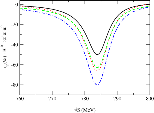
Figure 1: $CP$ violating asymmetry, $a_{CP}$, for $\bar{B}^{0}\rightarrow\pi^{+}\pi^{-}\pi^{0}$, for $k^{2}/m_{b}^{2}=0.3$, $N_{c}^{eff}=1.09(1.68)$ and limiting values of the CKM matrix elements for model $(1)$: solid line (dotted line) for $N_{c}^{eff}=1.09$ and max(min) CKM matrix elements. Dashed line (dot-dashed line) for $N_{c}^{eff}=1.68$ and max(min) CKM matrix elements.

A previous analysis [28] has been conducted showing the dependence on the CKM matrix elements and form factors of the direct $CP$ violating asymmetry. Here, we update our investigation by taking into account the latest values of the Wolfenstein CKM parameters, $\rho$ and $\eta$, and also by analysing more $B$ decays. In the following numerical calculations, we apply the formalism detailed previously and investigate $\bar{B}^{0}\rightarrow\pi^{+}\pi^{-}\pi^{0}$ more precisely. We find that for a fixed $N_{c}^{eff}$ there is a maximum value, $a_{max}$, for the $CP$ violating parameter, $a_{CP}$, when the invariant mass of the $\pi^{+}\pi^{-}$ pair is in the vicinity of the $\omega$ resonance. In Figs. 1 and 2, $CP$ violating asymmetries for $\bar{B}^{0}\rightarrow\pi^{+}\pi^{-}\pi^{0}$, for $k^{2}/m_{b}^{2}=0.3$ with $N_{c}^{eff}=1.09(1.68)$, and $k^{2}/m_{b}^{2}=0.5$ with $N_{c}^{eff}=1.11(1.80)$, are plotted, respectively, and for limiting values of CKM matrix elements. Graphic results are shown only for the model $(1)$, as an example. We have investigated five models, with five different form factors in order to test the model dependence of $a_{CP}$.

Concerning the maximum $CP$ violating asymmetry for $\bar{B}^{0}\rightarrow\pi^{+}\pi^{-}\pi^{0}$, $a_{max}$, it varies from $-51\%(-38\%)$ to $-84\%(-69\%)$ in the allowed range of $\rho,\eta$ for $k^{2}/m_{b}^{2}=0.3(0.5)$. From the numerical results listed in Table 3, for $N_{cmin}^{eff}=1.09(1.11)$ and $N_{cmax}^{eff}=1.68(1.80)$, we can see that the five models fall into two classes: models $(1,3)$ and $(5)$ and models $(2)$ and $(4)$. For models $(1,3)$ and $(5)$, and for $N_{cmin}^{eff}=1.09(1.11)$, the maximum asymmetry, $a_{max}$, is around $-54\%(-40\%)$ for the set $(\rho_{max},\eta_{max})$ and around $-69\%(-53.6\%)$ for the set $(\rho_{min},\eta_{min})$, leading to the ratio between them being around $1.28(1.34)$. In each of these models and for $N_{cmax}^{eff}=1.68(1.80)$, the maximum value of the asymmetry, $a_{max}$, varies from $-62.6\%(-48.6\%)$ for the set $(\rho_{max},\eta_{max})$ to around $-77.3\%(-64.6\%)$ for the set $(\rho_{min},\eta_{min})$. In that case, the ratio is equal to $1.23(1.32)$. If we consider models $(2)$ and $(4)$, the maximum asymmetry, $a_{max}$, where $N_{cmin}^{eff}=1.09(1.11)$, is around $-63.5\%(-48\%)$ for the set $(\rho_{max},\eta_{max})$ and around $-78.5\%(-62\%)$ for the set $(\rho_{min},\eta_{min})$. This yields a ratio $1.24(1.29)$. When $N_{cmax}^{eff}=1.68(1.80)$, one has a maximum asymmetry around $-71\%(-56.5\%)$ for the set $(\rho_{max},\eta_{max})$ and around $-84\%(-69\%)$ for the set $(\rho_{min},\eta_{min})$, leading to a ratio around $1.18(1.22)$.

From all these results, many comments can be enumerated. Although the maximum asymmetry, $a_{max}$, still varies over some range in the $\bar{B}^{0}\rightarrow\pi^{+}\pi^{-}\pi^{0}$ decay, we stress that by using more accurate CKM element values than before, a more precise $CP$ violating asymmetry is obtained. The reason is primarily the matrix elements $V_{td}$ and $V_{ub}$ which are involved in the $b\rightarrow d$ transition through the ratio of $p_{\omega}$ to $t_{\rho}$. In our previous $CP$ violation study [28] for the process $B^{-}\rightarrow\pi^{+}\pi^{-}\pi^{-}$, we found that the ratio between the maximum and minimum asymmetry, related to the minimum and maximum set of $(\rho,\eta)$, was around $1.6$. By comparison, in the present work, this ratio is reduced to $1.3$. The difference is related to the improvement in the measurement of the CKM matrix elements, and shows the strong effect of the CKM parameters, $\rho$ and $\eta$, on limiting asymmetry values.

With regard to the CKM matrix elements, it appears that if we take their upper limit, we obtain a smaller asymmetry, $a_{CP}$, and vice-versa. As we found before, there is still a strong dependence of the $CP$ violating asymmetry on the form factors. The difference between the two classes of models, $(1,3,5)$ and $(2,4)$, comes mainly from the magnitudes of the form factors. In fact, the form factor $F_{1}(k^{2})$, which describes the transition $B\rightarrow\pi$, is mainly responsible for this dependence. In both classes, we find a stronger dependence of the $CP$ violating asymmetry on the CKM matrix elements than that on the form factors or the effective parameter $N_{c}^{eff}$. The difference observed in our results between $k^{2}/m_{b}^{2}=0.3$ and $k^{2}/m_{b}^{2}=0.5$ arises from the $k^{2}$ dependence of the Wilson coefficients in the weak effective Hamiltonian. Finally, since $N_{c}^{eff}$ (treated as a free parameter) is related to hadronization effects through the factorization approach, it is not possible to determine its value accurately (since non-factorizable effects are not well known). That is why the asymmetry also varies in some range of $N_{c}^{eff}$. It is obvious that a more accurate value for $N_{c}^{eff}$ (which requires a more accurate approach with non-factorizable effects being taken into account), and hadronic decay form factors (which requires better understanding for pionic structure and the $B\rightarrow\pi$ transition) are needed in order to determine the CKM matrix elements.

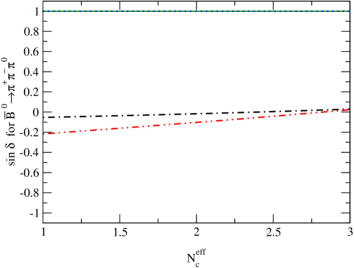
Figure 3: $\sin\delta$ as a function of $N_{c}^{eff}$, for $\bar{B}^{0}\rightarrow\pi^{+}\pi^{-}\pi^{0}$, for $k^{2}/m_{B}^{2}=0.3(0.5)$ and for model $(1)$. The solid (dotted) line at $\sin\delta=+1$ corresponds the case $\tilde{\Pi}_{\rho\omega}=(-3500;-300)$, where $\rho-\omega$ mixing is included. The dot-dashed (dot-dot-dashed) line corresponds to $\tilde{\Pi}_{\rho\omega}=(0;0)$, where $\rho-\omega$ mixing is not included.

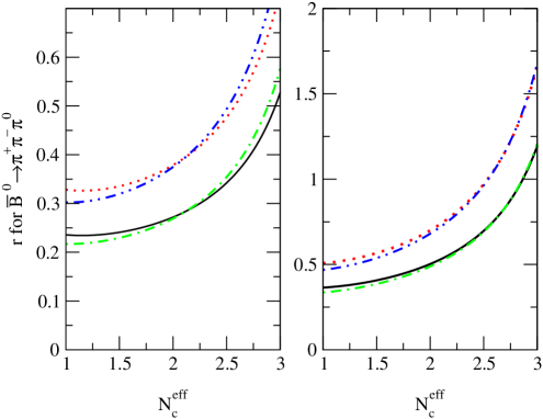
Figure 4: The ratio of penguin to tree amplitudes, $r$, as a function of $N_{c}^{eff}$, for $\bar{B}^{0}\rightarrow\pi^{+}\pi^{-}\pi^{0}$, for $k^{2}/m_{B}^{2}=0.3(0.5)$, for limiting values of the CKM matrix elements $(\rho,\eta)$ max(min), for $\tilde{\Pi}_{\rho\omega}=(-3500;-300)(0,0)$, (i.e. with(without) $\rho-\omega$ mixing) and for model $(1)$. Figure 4a (left): for $\tilde{\Pi}_{\rho\omega}=(0;0)$, solid line (dotted line) for $k^{2}/m_{B}^{2}=0.3$ and $(\rho,\eta)$ max(min). Dot-dashed line (dot-dot-dashed line) for $k^{2}/m_{B}^{2}=0.5$ and $(\rho,\eta)$ max(min). Figure 4b (right): same caption but for $\tilde{\Pi}_{\rho\omega}=(-3500;-300)$.

In spite of all the uncertainties mentioned above, we stress that the $\rho-\omega$ mixing mechanism in the $B\rightarrow\rho\pi$ decay can be used to remove ambiguity concerning the sign of $\sin\delta$. As the internal top quark dominates the $b\rightarrow d$ transition, the weak phase in the asymmetry is proportional to $\sin\alpha\;(=\sin\phi)$, where $\alpha={\rm arg}\left[-\frac{V_{td}V_{tb}^{\star}}{V_{ud}V_{ub}^{\star}}\right]$. Hence knowing the sign of $\sin\delta$ enables us to determine that of $\sin\alpha$ from a measurement of the asymmetry, $a_{CP}$. In Fig. 3 we show $\sin\delta$ as a function of $N_{c}^{eff}$ for $\bar{B}^{0}\rightarrow\pi^{+}\pi^{-}\pi^{0}$ when we have maximum $CP$ violation. Then, in our determined range of $N_{c}^{eff}$, ($1.09(1.11)<N_{c}^{eff}<1.68(1.80)$), one finds that its sign is always positive for all the models studied and for all the form factors. Therefore, by measuring the $CP$ violating asymmetry in $\bar{B}^{0}\rightarrow\pi^{+}\pi^{-}\pi^{0}$, we can remove the mod($\pi$) ambiguity which appears in the determination for $\alpha$ from the usual indirect measurements which yield $\sin 2\alpha$. In Fig. 4, the ratio of the penguin and tree amplitudes, as a function of $N_{c}^{eff}$, is plotted for limiting values of the CKM matrix elements, $\rho,\eta$, for the process $\bar{B}^{0}\rightarrow\pi^{+}\pi^{-}\pi^{0}$. Even though one gets a larger value of $\sin\delta$ around $N_{c}^{eff}=1$, for $\bar{B}^{0}\rightarrow\pi^{+}\pi^{-}\pi^{0}$, without $\rho-\omega$ mixing, one still has a small value for $r$ around this value of $N_{c}^{eff}$. In that case, the $CP$ violating asymmetry, $a_{CP}$, remains very small without $\rho-\omega$ mixing.

5 Branching ratios for $\boldsymbol{B^{\pm,0}\rightarrow\rho^{0}\pi^{\pm,0}}$

5.1 Formalism

The direct $B\rightarrow\rho^{0}\pi$ transition is the main contribution to the decay rate. In our case, to be consistent, we should also take into account the $\rho-\omega$ mixing contribution to the branching ratio, since we are working to the first order of isospin violation. The derivation is straightforward and we obtain the following form for the branching ratio for $B\rightarrow\rho^{0}\pi$:

$$BR(B\rightarrow\rho^{0}\pi)=\frac{G_{F}^{2}|\vec{p}_{\rho}|^{3}}{\alpha_{k}\pi\Gamma_{B}}\Bigg{|}\bigg{[}V_{d}^{T}A^{T}_{\rho^{0}}(a_{1},a_{2})-V_{d}^{P}A^{P}_{\rho^{0}}(a_{3},\cdots,a_{10})\bigg{]}\\ +\bigg{[}V_{d}^{T}A^{T}_{\omega}(a_{1},a_{2})-V_{d}^{P}A^{P}_{\omega}(a_{3},\cdots,a_{10})\bigg{]}\frac{\tilde{\Pi}_{\rho\omega}}{(s_{\rho}-m_{\omega}^{2})+im_{\omega}\Gamma_{\omega}}\Bigg{|}^{2}\ .$$ (28)

In Eq. (28) $G_{F}$ is the Fermi constant, $\Gamma_{B}$ is the $B$ total decay width, and $\alpha_{k}$ is an integer related to the given decay, $A^{T}_{V}$ and $A^{P}_{V}$ are the tree and penguin amplitudes, and $V_{d}^{T},V_{d}^{P}$ represent the CKM matrix elements involved in the tree and penguin diagrams, respectively:

$$V_{d}^{T}=|V_{ub}V_{ud}^{\star}|\ ,\;\;\;\;{\rm and}\;\;\;V_{d}^{P}=|V_{tb}V_{td}^{\star}|\ .$$ (29)

The effective parameters, $a_{i}$, which are involved in the decay amplitude, are the following combinations of effective Wilson coefficients:

$$a_{2j}=C_{2j}^{\prime}+\frac{1}{N_{c}^{eff}}C_{2j-1}^{\prime},\;\;\;a_{2j-1}=C_{2j-1}^{\prime}+\frac{1}{N_{c}^{eff}}C_{2j}^{\prime},\;\;{\rm for}\;\;j=1,\cdots,5\ .$$ (30)

5.2 Calculational details

In this section, we give full details of the theoretical decay amplitudes for decays involving the $b$ to $d$ transition. Two of these decays involve $\rho-\omega$ mixing. They are $B^{-}\rightarrow\rho^{0}\pi^{-}$ and $\bar{B}^{0}\rightarrow\rho^{0}\pi^{0}$. The other two decays are $\bar{B}^{0}\rightarrow\rho^{-}\pi^{+}$ and $B^{-}\rightarrow\rho^{-}\pi^{0}$. We list in the following, the tree and penguin amplitudes which appear in the given transitions.
For the decay $B^{-}\rightarrow\rho^{0}\pi^{-}$ ($\alpha_{k}=32$ in Eq. (28)),

$$\sqrt{2}A^{T}_{\rho}(a_{1},a_{2})=a_{1}f_{\rho}F_{1}(m_{\rho}^{2})+a_{2}f_{\pi}A_{0}(m_{\pi}^{2})\ ,\hskip 160.00024pt$$ (31)

$$\sqrt{2}A^{P}_{\rho}(a_{3},\cdots,a_{10})=f_{\rho}F_{1}(m_{\rho}^{2})\biggl{\{}-a_{4}+\frac{3}{2}(a_{7}+a_{9})+\frac{1}{2}a_{10}\biggr{\}}\\ +f_{\pi}A_{0}(m_{\pi}^{2})\Biggl{\{}a_{4}-2(a_{6}+a_{8})\biggl{[}\frac{m_{\pi}^{2}}{(m_{u}+m_{d})(m_{b}+m_{u})}\biggr{]}+a_{10}\Biggr{\}}\ ;$$ (32)

for the decay $B^{-}\rightarrow\omega\pi^{-}$ ($\alpha_{k}=32$ in Eq. (28)),

$$\sqrt{2}A^{T}_{\omega}(a_{1},a_{2})=a_{1}f_{\rho}F_{1}(m_{\rho}^{2})+a_{2}f_{\pi}A_{0}(m_{\pi}^{2})\ ,\hskip 160.00024pt$$ (33)

$$\sqrt{2}A^{P}_{\omega}(a_{3},\cdots,a_{10})=f_{\rho}F_{1}(m_{\rho}^{2})\biggl{\{}2(a_{3}+a_{5})+\frac{1}{2}(a_{7}+a_{9})+(a_{4}-\frac{1}{2}a_{10})\biggr{\}}\\ +f_{\pi}A_{0}(m_{\pi}^{2})\Biggl{\{}-2(a_{6}+a_{8})\biggl{[}\frac{m_{\pi}^{2}}{(m_{u}+m_{d})(m_{b}+m_{u})}\biggr{]}+a_{4}+a_{10}\Biggr{\}}\ ;$$ (34)

for the decay $\bar{B}^{0}\rightarrow\rho^{0}\pi^{0}$ ($\alpha_{k}=64$ in Eq. (28)),

$$2A^{T}_{\rho}(a_{1},a_{2})=a_{1}f_{\rho}F_{1}(m_{\rho}^{2})+a_{1}f_{\pi}A_{0}(m_{\pi}^{2})\ ,\hskip 170.00026pt$$ (35)

$$2A^{P}_{\rho}(a_{3},\cdots,a_{10})=f_{\rho}F_{1}(m_{\rho}^{2})\biggl{\{}-a_{4}+\frac{1}{2}(3a_{7}+3a_{9}+a_{10})\biggr{\}}+\\ f_{\pi}A_{0}(m_{\pi}^{2})\Biggl{\{}-a_{4}+(2a_{6}-a_{8})\biggl{[}\frac{m_{\pi}^{2}}{2m_{d}(m_{b}+m_{d})}\biggr{]}+\frac{1}{2}(-3a_{7}+3a_{9}+a_{10})\Biggr{\}}\ ;$$ (36)

for the decay $\bar{B}^{0}\rightarrow\omega\pi^{0}$ ($\alpha_{k}=64$ in Eq. (28)),

$$2A^{T}_{\omega}(a_{1},a_{2})=-a_{1}f_{\rho}F_{1}(m_{\rho}^{2})+a_{1}f_{\pi}A_{0}(m_{\pi}^{2})\ ,\hskip 170.00026pt$$ (37)

$$2A^{P}_{\omega}(a_{3},\cdots,a_{10})=f_{\rho}F_{1}(m_{\rho}^{2})\biggl{\{}-2(a_{3}+a_{5})-a_{4}-\frac{1}{2}(a_{7}+a_{9}-a_{10})\biggr{\}}\\ +f_{\pi}A_{0}(m_{\pi}^{2})\Biggl{\{}-a_{4}+(2a_{6}-a_{8})\biggl{[}\frac{m_{\pi}^{2}}{2m_{d}(m_{b}+m_{d})}\biggr{]}+\frac{1}{2}(-3a_{7}+3a_{9}+a_{10})\Biggr{\}}\ ;$$ (38)

for the decay $\bar{B}^{0}\rightarrow\rho^{-}\pi^{+}$ ($\alpha_{k}=16$ in Eq. (28)),

$$A^{T}_{\rho}(a_{1},a_{2})=a_{2}f_{\rho}F_{1}(m_{\rho}^{2})\ ,\hskip 230.00035pt$$ (39)

$$A^{P}_{\rho}(a_{3},\cdots,a_{10})=(a_{4}+a_{10})f_{\rho}F_{1}(m_{\rho}^{2})\ ;\hskip 180.00027pt$$ (40)

for the decay $B^{-}\rightarrow\rho^{-}\pi^{0}$ ($\alpha_{k}=32$ in Eq. (28)),

$${\sqrt{2}}A^{T}_{\rho}(a_{1},a_{2})=a_{2}f_{\rho}F_{1}(m_{\rho}^{2})+a_{1}f_{\pi}A_{0}(m_{\pi}^{2})\ ,\hskip 160.00024pt$$ (41)

$${\sqrt{2}}A^{P}_{\rho}(a_{3},\cdots,a_{10})=f_{\rho}F_{1}(m_{\rho}^{2})(a_{4}+a_{10})+\\ f_{\pi}A_{0}(m_{\pi}^{2})\Biggl{\{}-a_{4}-\frac{1}{2}(3a_{7}-3a_{9}-a_{10})+(2a_{6}-a_{8})\biggl{[}\frac{m_{\pi}^{2}}{2m_{d}(m_{b}+m_{d})}\biggr{]}\Biggr{\}}\ .$$ (42)

Moreover, we can calculate the ratio between two branching ratios, namely $BR(B^{0}\rightarrow\rho^{\pm}\pi^{\mp})$ and $BR(B^{\pm}\rightarrow\rho^{0}\pi^{\pm})$, in which the uncertainty caused by many systematic errors is removed. We define the ratio, $R_{\pi}$, as:

$$R_{\pi}=\frac{BR(B^{0}\rightarrow\rho^{\pm}\pi^{\mp})}{BR(B^{\pm}\rightarrow\rho^{0}\pi^{\pm})}\ .$$ (43)

5.3 Numerical results

The numerical values for the CKM matrix elements $V_{d}^{T,P}$, $\rho-\omega$ mixing amplitude $\tilde{\Pi}_{\rho\omega}$, and particle masses $m_{V,P}$, which appear in Eq. (28), have been reported in Sections 2.2 and 3. The Fermi constant is taken to be $G_{F}=1.166391\times 10^{-5}{\rm GeV}^{-2}$ [14], and for the total decay width $B$ meson, $\Gamma_{B}(=1/\tau_{B})$, we use the world average $B$ life-time values (combined results from ALEPH, CDF, DELPHI, L3, OPAL and SLD) [21]:

$$\tau_{B^{0}} =1.546\pm 0.021\;{\rm ps}\ ,$$

$$\tau_{B^{+}} =1.647\pm 0.021\;{\rm ps}\ .$$ (44)

To compare theoretical results with experimental data, as well as to determine constraints on the effective number of colours, $N_{c}^{eff}$, the form factors and the CKM matrix parameters, we shall use the experimental branching ratios collected by CLEO [29], BELLE [30, 31, 32] and BABAR [33, 34] factories. All the experimental values are summarized in Table 4.

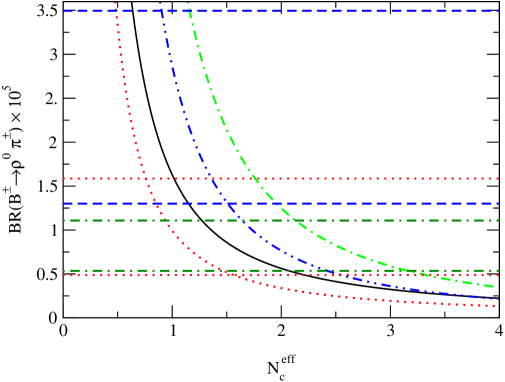
Figure 5: Branching ratio for $B^{\pm}\rightarrow\rho^{0}\pi^{\pm}$ for models $1(2)$, $k^{2}/m_{B}^{2}=0.3$ and limiting values of the CKM matrix elements. Solid line (dotted line) for model $(1)$ and max(min) CKM matrix elements. Dot-dashed line (dot-dot-dashed line) for model $(2)$ and max(min) CKM matrix elements. Horizontal dotted lines: CLEO data; horizontal dashed lines: BABAR data; horizontal dot-dashed lines: BELLE data.

In order to determine the range of $N_{c}^{eff}$, which is allowed by experimental data, we have calculated the branching ratios for $B^{\pm}\rightarrow\rho^{0}\pi^{\pm}$, $B^{\pm}\rightarrow\rho^{\pm}\pi^{0}$, $B^{0}\rightarrow\rho^{\pm}\pi^{\mp}$, and $B^{0}\rightarrow\rho^{0}\pi^{0}$. All the results are shown in Figs. 5, 6, 7 and 8 for the corresponding branching ratios listed above. Results are plotted for models $(1)$ and $(2)$, since they involve different form factor values and thus show their dependence on form factors. As experimental data, we shall use three sets of data from the CLEO, BABAR and BELLE Collaborations, respectively. Since experimental branching ratios from CLEO are the most accurate, we shall use them to extract the range of $N_{c}^{eff}$. The other two, the BABAR and BELLE data, will give us an idea of the magnitude of the experimental uncertainties. It is clear that numerical results are very sensitive to uncertainties coming from the experimental data. Thus, the determination of the allowed range of $N_{c}^{eff}$ will be done by using all the branching ratio results.

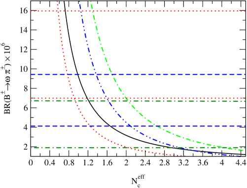
Figure 9: Branching ratio for $B^{\pm}\rightarrow\omega\pi^{\pm}$ for models $1(2)$, $k^{2}/m_{B}^{2}=0.3$ and limiting values of the CKM matrix elements. Solid line (dotted line) for model $(1)$ and max(min) CKM matrix elements. Dot-dashed line (dot-dot-dashed line) for model $(2)$ and max(min) CKM matrix elements. Same notation for experimental data as in Fig. 5.

Let us start with the decay processes $B^{-}\rightarrow\rho^{0}\pi^{-}$ and $B^{-}\rightarrow\rho^{-}\pi^{0}$. In both cases, there is a large range of acceptable values for $N_{c}^{eff}$ and the CKM matrix elements over which the theoretical results are consistent with experimental data from CLEO, BABAR and BELLE. For $B^{-}\rightarrow\rho^{-}\pi^{0}$, the lack of data does not allow us to determine the range. However, experiment and theory are consistent in both cases. For $B^{-}\rightarrow\rho^{0}\pi^{-}$, the models show considerable variation even though they are all consistent with the experimental data. Numerical results for models $(1,3)$ and $(5)$ are close, so are those for models $(2)$ and $(4)$. We emphasise that the effect of $\rho-\omega$ mixing on the branching ratio $B^{\pm}\rightarrow\rho^{0}\pi^{\pm}$ can be as large as $30\%$. As regards $B^{0}\rightarrow\rho^{-}\pi^{+}$ and $\bar{B}^{0}\rightarrow\rho^{0}\pi^{0}$, the results and conclusions are different from those for $B^{-}\rightarrow\rho^{0}\pi^{-}$. If we look at the branching ratio for $B^{0}\rightarrow\rho^{\pm}\pi^{\mp}$, only models $(2)$ and $(4)$ are consistent with experimental data over a large range of $N_{c}^{eff}$, whereas models $(1,3)$ and $(5)$ are not. The strong sensitivity to the results in that case comes from the fact that the decay branching ratios for $B^{0}\rightarrow\rho^{\pm}\pi^{\mp}$ depend on form factors more sensitively, because in this case only one form factor, $F_{1}(k^{2})$, is involved. In all the other cases, the amplitudes depend on both $F_{1}(k^{2})$ and $A_{0}(k^{2})$. Therefore these branching ratios are less sensitive to the magnitude of the form factors. Finally, for the branching ratio $BR(B^{\pm}\rightarrow\omega\pi^{\pm})$ plotted in Fig. 9, all models give theoretical results consistent with experimental data. Once again, the difference observed between models $(1)$ and $(2)$ mainly comes from the form factor $F_{1}(k^{2})$ (i.e. from the pion wave function used). Our analysis shows that models $(1,3)$ and $(5)$ cannot give results consistent with all experiments and have to be excluded.

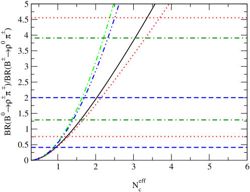
Figure 10: The ratio of two $\rho\pi$ branching ratios versus $N_{c}^{eff}$ for models $1(2)$ and for limiting values of the CKM matrix elements: solid line (dotted line) for model $(1)$ with max(min) CKM matrix elements. Dot-dashed line (dot-dot-dashed line) for model $(2)$ with max(min) CKM matrix elements. Same notation for experimental data as in Fig. 5.

To remove systematic uncertainties coming from experimental results, one can calculate the ratio between two branching ratios for $B$ decays. In the present case (with the data available), the ratio, $R_{\pi}$, is between $BR(B^{\pm}\rightarrow\rho^{0}\pi^{\pm})$ and $BR(B^{0}\rightarrow\rho^{\pm}\pi^{\mp})$. Results are shown in Fig. 10. We observe that the ratios differ totally from each other for models $(1,3)$ and $(5)$ and models $(2)$ and $(4)$. Since models $(1,3)$ and $(5)$ have already been excluded, we will use models $(2)$ and $(4)$ for the determination of the range for $N_{c}^{eff}$. If we just include tree contributions in the decay amplitudes, $R_{\pi}$ becomes independent of the CKM matrix elements. Penguin contributions lead to a relatively weak dependence of $R_{\pi}$ on the CKM matrix elements. By comparing numerical results and experimental data, we are now able to extract a range for $N_{c}^{eff}$ which is consistent with all the results. To determine the best range of $N_{c}^{eff}$, we select the values of $N_{c}^{eff}$ which are allowed by all constraints for each model. Finally, after excluding models $(1,3)$ and $(5)$ for the obvious reasons mentioned before, we can now fix the upper and the lower limit of the range of $N_{c}^{eff}$ (Table 5). We find that $N_{c}^{eff}$ should be in the range $1.09(1.11)<N_{c}^{eff}<1.68(1.80)$ for $k^{2}/m_{b}^{2}=0.3(0.5)$. Comparing with our previous study, the current range of $N_{c}^{eff}$ is consistent but smaller than the previous one.

6 Summary and discussion

The first aim of the present work was to compare theoretical branching ratios for $B^{\pm}\rightarrow\rho^{0}\pi^{\pm}$, $B^{\pm}\rightarrow\rho^{\pm}\pi^{0}$, $B^{0}\rightarrow\rho^{\pm}\pi^{\mp}$ and $B^{0}\rightarrow\rho^{0}\pi^{0}$ with experimental data from the CLEO, BABAR and BELLE Collaborations. The second was to apply recent values of the CKM matrix elements, e.g. $A,\lambda,\eta$ and $\rho$, to study direct $CP$ violation for $B$ decay such as $\bar{B}^{0}\rightarrow\rho^{0}(\omega)\pi^{0}\rightarrow\pi^{+}\pi^{-}\pi^{0}$, where the $\rho-\omega$ mixing mechanism must be included. The advantage of including $\rho-\omega$ mixing is that the strong phase difference which is necessary for direct $CP$ violation, is large and rapidly varying near the $\omega$ resonance. As a result, the $CP$ violating asymmetry, $a_{CP}$, reaches a maximum, $a_{max}$, when the invariant mass of the $\pi^{+}\pi^{-}$ pair is in the vicinity of the $\omega$ resonance and $\sin\delta=+1$ at this point.

In our approach, we started from the weak effective Hamiltonian where short distance and long distance physics are separated and treated by a perturbative approach (Wilson coefficients) and a non-perturbative approach (operator product expansion), respectively. One of the main uncertainties introduced in our calculation comes from the hadronic matrix elements for both tree and penguin operators. We treated them by applying a naive factorization approximation, where $N_{c}^{eff}$ is taken as an effective parameter. Although this is clearly an approximation, it has been pointed out [35] that it may be quite reliable in energetic weak decays such as $B\rightarrow\rho\pi$.

We have investigated the direct $CP$ violating asymmetry in the $B$ decay: $\bar{B}^{0}\rightarrow\pi^{+}\pi^{-}\pi^{0}$. We found that the $CP$ violation parameter, $a_{CP}$, is very sensitive to the parameters $\rho$ and $\eta$ in the CKM matrix, and also to the magnitude of the form factors appearing in the five phenomenological models we investigated. We have calculated the maximum asymmetry, $a_{max}$, as a function of the effective parameter, $N_{c}^{eff}$, with the limiting values of the CKM matrix elements. We found that the $CP$ violating asymmetry, $a_{max}$, can vary from $-37\%$ to $-84\%$ over all the models $(1,2,3,4,5)$. As we already suggested in a previous study [28], the ratio between the asymmetries for limiting values of the CKM matrix elements is mainly governed by $\eta$. Previously, we found a ratio equal to $1.64$ where the CKM values used were the following: $A=0.815,\lambda=0.2205$, $0.09<\rho<0.254$, and $0.323<\eta<0.442$. In the present work, we found for the same decay, a ratio equal to $1.30$. The more accurate value for $\eta$ has reduced uncertainties on both the $CP$ violating asymmetry and the ratio, $\Gamma(B^{\pm}\rightarrow\rho^{0}\pi^{\pm})/\Gamma(B^{0}\rightarrow\rho^{0}\pi^{0})$.

Moreover, we stressed that without the $\rho-\omega$ mixing mechanism, the $CP$ violating asymmetry, $a_{CP}$ (which is proportional to both $\sin\delta$ and $r$), is small since in that case either $\sin\delta$ or $r$ is small. In the allowed range of $N_{c}^{eff}$, we also found that the sign of $\sin\delta$ is always positive. Therefore, by measuring $a_{CP}$, we can remove the phase mod($\pi$) ambiguity which occurs in the usual method for the determination of the CKM unitarity angle $\alpha$.

We have calculated branching ratios for $B^{\pm}\rightarrow\rho^{0}\pi^{\pm}$, $B^{\pm}\rightarrow\rho^{\pm}\pi^{0}$, $B^{0}\rightarrow\rho^{\pm}\pi^{\mp}$ and $B^{0}\rightarrow\rho^{0}\pi^{0}$ and compared the results with experimental data coming from the CLEO, BABAR and BELLE Collaborations. We have shown that for models $(2)$ and $(4)$ there is a range for $N_{c}^{eff}$, $1.09(1.11)<N_{c}^{eff}<1.68(1.80)$, in which theoretical results are consistent with experimental data. Models $(1,3)$ and $(5)$ are excluded since the form factor $F_{1}(k^{2})$ in these models cannot produce results consistent with experiment. For a deeper investigation into this problem, some resonant and non-resonant contributions [36, 37] which may carry bigger effects than expected in the calculation of branching ratios in $\rho\pi$ may have to be considered seriously.

With more accurate CKM matrix elements values, e.g. $\rho$ and $\eta$, we are able to give more precise $CP$ violating asymmetries, and the main uncertainties remaining are from the factorization [3] approach and the hadronic decay form factors. In the future one may hope to use QCD factorization to replace the effective parameter, $N_{c}^{eff}$, and hence to provide a more reliable treatment of non-factorizable effects. With regard to form factors, we have shown that some models for the $B\rightarrow\pi$ transition are not consistent with the experimental branching ratios. We expect that our predictions will provide useful guidance for future investigations in $B$ decays. We look forward to even more accurate experimental data from our experimental colleagues in order to further constrain our theoretical results and hence, to further advance the determination of the CKM parameters $\rho$ and $\eta$ and our understanding of $CP$ violation within or beyond the Standard Model.

Acknowledgements

This work was supported in part by the Australian Research Council and the University of Adelaide.

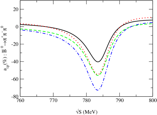
Figure 2: $CP$ violating asymmetry, $a_{CP}$, for $\bar{B}^{0}\rightarrow\pi^{+}\pi^{-}\pi^{0}$, for $k^{2}/m_{b}^{2}=0.5$, $N_{c}^{eff}=1.11(1.80)$ and limiting values of the CKM matrix elements for model $(1)$: solid line (dotted line) for $N_{c}^{eff}=1.11$ and max(min) CKM matrix elements. Dashed line (dot-dashed line) for $N_{c}^{eff}=1.80$ and max(min) CKM matrix elements.

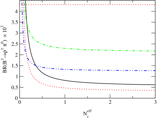
Figure 6: Branching ratio for $B^{\pm}\rightarrow\rho^{\pm}\pi^{0}$ for models $1(2)$, $k^{2}/m_{B}^{2}=0.3$ and limiting values of the CKM matrix elements. Solid line (dotted line) for model $(1)$ and max(min) CKM matrix elements. Dot-dashed line (dot-dot-dashed line) for model $(2)$ and max(min) CKM matrix elements. Same notation for experimental data as in Fig. 5.

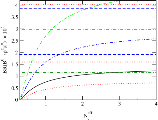
Figure 7: Branching ratio for $B^{0}\rightarrow\rho^{\pm}\pi^{\mp}$ for models $1(2)$, $k^{2}/m_{B}^{2}=0.3$ and limiting values of the CKM matrix elements. Solid line (dotted line) for model $(1)$ and max(min) CKM matrix elements. Dot-dashed line (dot-dot-dashed line) for model $(2)$ and max(min) CKM matrix elements. Same notation for experimental data as in Fig. 5.

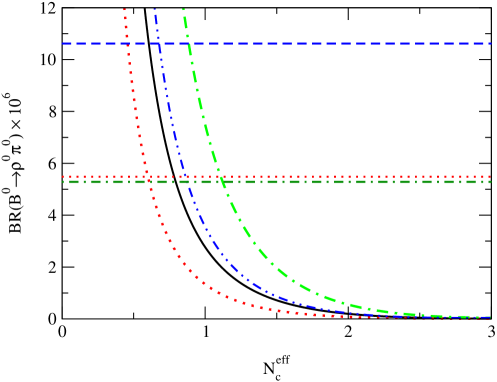
Figure 8: Branching ratio for $B^{0}\rightarrow\rho^{0}\pi^{0}$ for models $1(2)$, $k^{2}/m_{B}^{2}=0.3$ and limiting values of the CKM matrix elements. Solid line (dotted line) for model $(1)$ and max(min) CKM matrix elements. Dot-dashed line (dot-dot-dashed line) for model $(2)$ and max(min) CKM matrix elements. Same notation for experimental data as in Fig. 5.

$C_{i}^{\prime}$	$q^{2}/m_{b}^{2}=0.3$	$q^{2}/m_{b}^{2}=0.5$
$C_{1}^{\prime}$	$-0.3125$	$-0.3125$
$C_{2}^{\prime}$	$+1.1502$	$+1.1502$
$C_{3}^{\prime}$	$+2.433\times 10^{-2}+1.543\times 10^{-3}i$	$+2.120\times 10^{-2}+2.174\times 10^{-3}i$
$C_{4}^{\prime}$	$-5.808\times 10^{-2}-4.628\times 10^{-3}i$	$-4.869\times 10^{-2}-1.552\times 10^{-2}i$
$C_{5}^{\prime}$	$+1.733\times 10^{-2}+1.543\times 10^{-3}i$	$+1.420\times 10^{-2}+5.174\times 10^{-3}i$
$C_{6}^{\prime}$	$-6.668\times 10^{-2}-4.628\times 10^{-3}i$	$-5.729\times 10^{-2}-1.552\times 10^{-2}i$
$C_{7}^{\prime}$	$-1.435\times 10^{-4}-2.963\times 10^{-5}i$	$-8.340\times 10^{-5}-9.938\times 10^{-5}i$
$C_{8}^{\prime}$	$+3.839\times 10^{-4}$	$+3.839\times 10^{-4}$
$C_{9}^{\prime}$	$-1.023\times 10^{-2}-2.963\times 10^{-5}i$	$-1.017\times 10^{-2}-9.938\times 10^{-5}i$
$C_{10}^{\prime}$	$+1.959\times 10^{-3}$	$+1.959\times 10^{-3}$

Table 1: Effective Wilson coefficients for the tree operators, electroweak and QCD penguin operators (see Refs [11, 12]).

	$h_{A_{0}}$	$h_{1}$	$m_{A_{0}}$	$m_{1}$	$d_{0}(d_{1})$	$b_{0}(b_{1})$
model $(1)$	0.280	0.290	5.27	5.32
model $(2)$	0.340	0.625	5.27	5.32
model $(3)$	0.280	0.290	5.27	5.32
model $(4)$	0.340	0.625	5.27	5.32
model $(5)$	0.372	0.305			1.400(0.266)	0.437(-0.752)

Table 2: Form factor values for $B\rightarrow\rho$ and $B\rightarrow\pi$ at $q^{2}=0$.

	$N_{cmin}^{eff}=1.09(1.11)$	$N_{cmax}^{eff}=1.68(1.80)$
model $(1)$
$\rho_{max},\eta_{max}$	-55(-41)	-65(-51)
$\rho_{min},\eta_{min}$	-72(-55)	-80(-65)
model $(2)$
$\rho_{max},\eta_{max}$	-63(-48)	-71(-56)
$\rho_{min},\eta_{min}$	-78(-62)	-84(-69)
model $(3)$
$\rho_{max},\eta_{max}$	-56(-41)	-65(-51)
$\rho_{min},\eta_{min}$	-72(-55)	-80(-69)
model $(4)$
$\rho_{max},\eta_{max}$	-64(-48)	-71(-57)
$\rho_{min},\eta_{min}$	-79(-62)	-84(-69)
model $(5)$
$\rho_{max},\eta_{max}$	-51(-38)	-58(-44)
$\rho_{min},\eta_{min}$	-63(-51)	-72(-60)

Table 3: Maximum $CP$ violating asymmetry $a_{max}(\%)$ for $\bar{B}^{0}\rightarrow\pi^{+}\pi^{-}\pi^{0}$, for all models, limiting (upper and lower) values of the CKM matrix elements, and $k^{2}/m_{b}^{2}=0.3(0.5)$.

	CLEO	BABAR	BELLE
$\rho^{0}\pi^{\pm}$	${10.4^{+3.3}_{-3.4}\pm 2.1}^{\star}$	${24\pm 8\pm 3}^{\Box}$ $(\leq 39)^{\P}$	${8.0^{+2.3+0.7}_{-2.0-0.7}}^{\star}$ $(\leq 28.8)^{\P}$
$\rho^{\pm}\pi^{0}$	$\leq{43}^{\P}$	$-$	$-$
$\rho^{\pm}\pi^{\mp}$	${27.6^{+8.4}_{-7.4}\pm 4.2}^{\star}$	${28.9\pm 5.4\pm 4.3}^{\star}$	${20.8^{+6.0+2.8}_{-6.3-3.1}}^{\star}$ $(\leq 35.7)^{\P}$
$\rho^{0}\pi^{0}$	${1.6^{+2.0}_{-1.4}\pm 0.8}^{\bullet}$ $(\leq{5.5})^{\P}$	$\leq{10.6}^{\P}$	$\leq 5.3^{\P}$
$\frac{BR(\rho^{\pm}\pi^{\mp})}{BR(\rho^{0}\pi^{\pm})}$	$2.65\pm 1.9$	$1.20\pm 0.79$	$2.60\pm 1.31$
$\omega\pi^{\pm}$	${11.3^{3.3}_{-2.9}\pm 1.4}^{\star}$	${6.6^{2.1}_{-1.8}\pm 0.7}^{\star}$	${4.2^{2.0}_{-1.8}\pm 0.5}^{\star}$

Table 4: The branching ratios measured by CLEO, BABAR and BELLE factories for $B$ decays into $\rho\pi$ in unit of $10^{-6}$ (see Ref in text). ${\rm Experimental\;data}^{\star}$, ${\rm preliminary\;results}^{\Box}$, ${\rm fit}^{\bullet}$ and ${\rm upper\;limit}^{\P}$.

$B\rightarrow\rho\pi$	$\left\{N_{c}^{eff}\right\}$ with mixing
model $(2)$	1.09;1.63(1.12;1.77)
model $(4)$	1.10;1.68(1.11;1.80)
maximum range	1.09;1.68(1.11;1.80)
minimum range	1.10;1.63(1.12;1.77)

Table 5: Best range of $N_{c}^{eff}$ determined for $k^{2}/m_{b}^{2}=0.3(0.5)$ and for all $B\rightarrow\rho\pi$ decays.

References

- [1] A.B. Carter and A.I. Sanda, Phys. Rev. Lett. 45 (1980) 952, Phys. Rev. D23 (1981) 1567; I.I. Bigi and A.I. Sanda, Nucl. Phys. B193 (1981) 85.
- [2] Proceedings of the Workshop on CP Violation, Adelaide 1998, edited by X.-H. Guo, M. Sevior and A.W. Thomas (World Scientific, Singapore).
- [3] M. Beneke, G. Buchalla, M. Neubert and C.T. Sachrajda, Nucl. Phys. B591 (2000) 313.
- [4] R. Enomoto and M. Tanabashi, Phys. Lett. B386 (1996) 413.
- [5] S. Gardner, H.B. O’Connell and A.W. Thomas, Phys. Rev. Lett. 80 (1998) 1834.
- [6] X.-H. Guo and A.W. Thomas, Phys. Rev. D58 (1998) 096013, Phys. Rev. D61 (2000) 116009.
- [7] G. Buchalla, A.J. Buras and M.E. Lautenbacher, Rev. Mod. Phys. 68, (1996) 1125.
- [8] A.J. Buras, Lect. Notes Phys. 558 (2000) 65, Also in ‘Recent Developments in Quantum Field Theory’, Springer Verlag, eds. P. Breitenlohner, D. Maison and J. Wess, hep-ph/9901409.
- [9] A.J. Buras, Published in ‘Probing the Standard Model of Particle Interactions’, eds. 1998, Elsevier Science B.V., hep-ph/9806471.
- [10] N.G. Deshpande and X.-G. He, Phys. Rev. Lett. 74 (1995) 26.
- [11] R. Fleischer, Int. J. Mod. Phys. A12 (1997) 2459, Z. Phys. C62 (1994) 81, Z. Phys. C58 (1993) 483.
- [12] G. Kramer, W. Palmer and H. Simma, Nucl. Phys. B428 (1994) 77.
- [13] O. Leitner. X.-H. Guo and A.W. Thomas, hep-ph/0208198, published in Phys. Rev. D.
- [14] The Particle Data Group, D.E. Groom et al., Eur. Phys. J. C15 (2000) 1.
- [15] H.B. O’Connell, B.C. Pearce, A.W. Thomas and A.G. Williams, Prog. Part. Nucl. Phys. 39 (1997) 201; H.B. O’Connell, A.G. Williams, M. Bracco and G. Krein, Phys. Lett. B370 (1996) 12; H.B. O’Connell, Aust. J. Phys. 50 (1997) 255.
- [16] H.B. O’Connell, A.W. Thomas and A.G. Williams, Nucl. Phys. A623 (1997) 559; K. Maltman, H.B. O’Connell and A.G. Williams, Phys. Lett. B376 (1996) 19.
- [17] S. Gardner and H.B. O’Connell, Phys. Rev. D57 (1998) 2716.
- [18] J. Schwinger, Phys. Rev. 12 (1964) 630; D. Farikov and B. Stech, Nucl. Phys. B133 (1978) 315; N. Cabibbo and L. Maiani, Phys. Lett. B73 (1978) 418; M.J. Dugan and B. Grinstein, Phys. Lett. B255 (1991) 583.
- [19] M. Bauer, B. Stech and M. Wirbel, Z. Phys. C34 (1987) 103; M. Wirbel, B. Stech and M. Bauer, Z. Phys. C29 (1985) 637.
- [20] L. Wolfenstein, Phys. Rev. Lett. 51 (1983) 1945, Phys. Rev. Lett. 13 (1964) 562.
- [21] By ALEPH Collaboration, CDF Collaboration, DELPHI Collaboration, L3 Collaboration, OPAL Collaboration and SLD Collaboration (D. Abbaneo et al.), hep-ex/0112028.
- [22] H.-Y. Cheng and A. Soni, Phys. Rev. D64 (2001) 114013.
- [23] X.-H. Guo and T. Huang, Phys. Rev. D43 (1991) 2931.
- [24] P. Ball, JHEP 9809 (1998) 005.
- [25] P. Ball and V.M. Braun, Phys. Rev. D58 (1998) 094016.
- [26] Y.-H. Chen, H.-Y. Cheng, B. Tseng and K.-C. Yang, Phys. Rev. D60 (1999) 094014.
- [27] D. Melikhov and B. Stech, Phys. Rev. D62 (2000) 014006.
- [28] X.-H. Guo, O. Leitner and A.W. Thomas, Phys. Rev. D63 (2001) 056012.
- [29] C.P. Jessop, et al. (CLEO Collaboration), Phys. Rev. Lett. 85 (2000) 2881.
- [30] A. Bozek (BELLE Collaboration), in Proceedings of the 4th International Conference on B Physics and CP Violation, Ise-Shima, Japan, February 2001, hep-ex/0104041.
- [31] K. Abe, et al. (BELLE Collaboration), in Proceedings of the XX International Symposium on Lepton and Photon Interactions at High Energies, July 2001, Roma, Italy, BELLE-CONF-0115 (2001).
- [32] K. Abe, et al. (BELLE Collaboration), Phys. Rev. D65 (2002) 092005; A. Gordon, et al. (BELLE Collaboration), hep-ex/0207007 (submitted to Elsevier); R.S. Lu, et al. (BELLE Collaboration), hep-ex/0207019 (Submitted to Phys. Rev. Lett.).
- [33] T. Schietinger (BABAR Collaboration), Proceedings of the Lake Louise Winter Institute on Fundamental Interactions, Alberta, Canada, February 2001, hep-ex/0105019.
- [34] B. Aubert, et al. (BABAR Collaboration), hep-ex/0008058; B. Aubert, et al. (BABAR Collaboration), Phys. Rev. Lett. 87 (2000) 221802.
- [35] H.-Y. Cheng, Phys. Lett. B335 (1994) 428, Phys. Lett. B395 (1997) 345; H.-Y. Cheng and B. Tseng, Phys. Rev. D58 (1998) 094005.
- [36] Ulf-G. Meissner, hep-ph/0206125; A. Deandrea, hep-ph/0005014.
- [37] J. Tandean and S. Gardner, Phys. Rev. D66 (2002) 034019; S. Gardner and Ulf-G. Meissner, Phys. Rev. D65 (2002) 094004; A. Deandrea and A.D. Polosa, Phys. Rev. Lett. 86 (2001) 216-219.