Delocalized Operator Expansion

Abstract

A generalization of Wilson’s local OPE for the short-distance expansion of Euclidean current correlators, called delocalized operator expansion (DOE), which has been proposed recently, is discussed. The DOE has better convergence properties than the OPE and can account for non-local non-perturbative QCD effects.

1 INTRODUCTION - WILSON’S OPE

The Wilson OPE is one of the standard tools in modern hadronic physics. The OPE provides the framework for systematically separating short-distance contributions ($x\ll\Lambda^{-1}$) from long-distance contributions ($x\sim\Lambda^{-1}$). For illustration consider the large-momentum expansion of the correlator of a gauge-invariant QCD current $j(x)$ [2],

$$i\int\!d^{4}xe^{iqx}\langle Tj(x)j^{\dagger}(0)\rangle\stackrel{{\scriptstyle Q^{2}=-q^{2}\to\infty}}{{\longrightarrow}}$$ (1)

$$\mbox{\hskip 36.98857pt}Q^{2}\sum_{N=0}\sum_{l=1}^{l_{N}}\,c_{Nl}(Q^{2})\,\langle O_{Nl}(0)\rangle\,$$

where $N$ runs over the dimension of the local and gauge-invariant composite operators $O_{Nl}(0)$, and $l$ labels operators of the same dimensions. The long-distance fluctuations are encoded in the matrix elements $\langle O_{Nl}(0)\rangle$, also called condensates, and the short-distance contributions are contained in the Wilson coefficients $c_{Nl}(Q^{2})$. One has the scaling $\langle O_{Nl}(0)\rangle\sim\Lambda^{N}$ and $c_{Nl}(Q^{2})\sim Q^{-N}$. The $N=0$ term is entirely perturbative and higher order terms in the series are of order $(\Lambda/Q)^{N}$. For the case $Q\gg\Lambda$ the expansion should be reasonably well-behaved, but it is known to be asymptotic. There are situations where the OPE cannot be applied or where it cannot give definite answers. When $Q$ approaches $\Lambda$, the series breaks down. The OPE can also not answer questions related to the asymptotics of the series due to the truncation of the series. In this talk I discuss a generalization of the local OPE that has been proposed in Ref. [3] and has been called ”Delocalized Operator Expansion” (DOE). The DOE is an attempt to combine the advantages of the OPE with methods that might be useful to resolve issues that cannot be tackled easily in the framework of the OPE.

2 BASIC FRAMEWORK

Given the exact knowledge of (nonlocal) gauge-invariant QCD vacuum correlators and assuming for now that perturbative propagation can be factorized unambiguously from nonperturbative fluctuations, one may view the OPE as the multipole expansion of the perturbative part. To see this, let us consider the simplified case of a nonperturbative and nonlocal dimension-4 structure $g(x)$ corresponding to a slowly varying 2-point correlator falling off at distance $\Delta_{g}\sim\Lambda^{-1}$ in its Euclidean space-time argument $x$. In addition, we consider a perturbative short-distance function $f(x)$, that probes the vacuum at distance $x\sim\Delta_{f}\sim Q^{-1}$. For $Q\gg\Lambda$, $f(x)$ is strongly peaked compared to $g(x)$ (see Fig. 1).

Figure 1: Schematic picture of the short-distance function $f(x)$ and the 2-point-correlator $g(x)$ illustrating the scale hierarchy $\Delta_{f}/\Delta_{g}\sim\Lambda/Q\ll 1$.

For illustration I consider the problem in one dimension. Then the chain of local power corrections to the perturbative result is obtained from the expression

$$\textstyle\int_{-\infty}^{\infty}dx\,f(x)\,g(x)=:(f,g)\,,$$ (2)

which is the bilinear form in the dual space spanned by strongly peaked functions such as $f$ and slowly varying functions such as $g$. The generalization to more than one dimension, which also allows the treatment of non-perturbative $n$-point correlators, is straightforward. In the OPE $f(x)$ is expanded in analogy to the multipole expansion of a localized charge distribution in electrostatics. This can be formulated by introducing the dual space basis functions ($n=0,\ldots,\infty$)

$$\textstyle e_{n}(x)\equiv\frac{(-1)^{n}}{n!}\,\delta^{(n)}(x)\,,\quad\tilde{e}_{n}(x)\equiv x^{n}\,,$$ (3)

with the orthonormality relation $(e_{n},\tilde{e}_{m})=\delta_{nm}$. The multipole expansion of $f(x)$ then reads

$$\textstyle f(x)=\sum_{n=0}^{\infty}(f,\tilde{e}_{n})e_{n}(x)$$ (4)

which leads to

$$\int\!\!\!dxf(x)g(x)=\sum_{n=0}^{\infty}(f,\tilde{e}_{n})(e_{n},g)=:\sum_{n=0}^{\infty}\!f_{n}g_{n}.$$ (5)

The $f_{n}$’s are the Wilson coefficients and the $g_{n}$ the matrix elements of operators obtained from locally expanding the field content in the correlator $g(x)$ for small $x$. In momentum space representation the Wilson coefficients and matrix elements have the generic form

$$\textstyle f_{n}=(i\frac{d}{dk})^{n}\,\tilde{f}(k)|_{k=0}\,,\,\,g_{n}=\int\frac{dk}{2\pi}\,\frac{(ik)^{n}}{n!}\,\tilde{g}(k)\,,$$ (6)

where $\tilde{f}$ and $\tilde{g}$ are the Fourier transforms of $f$ and $g$, respectively.

Briefly switching to 4 dimensions, a simple example for the function $g(x)$ is the gauge invariant field strength correlator [4]

$$g_{\tiny\mu\nu\kappa\lambda}(x)\!\equiv\!\mbox{Tr}\langle g^{2}G_{\mu\nu}(x)S(x,0)G_{\kappa\lambda}(0)S(0,x)\rangle,$$ (7)

where

$$\textstyle S(x,y)\,=\,{\cal P}\,\exp\{ig\int_{0}^{x}dz_{\mu}A_{\mu}(z)\}\,.$$ (8)

It generates the following chain of vacuum expectation values (VEV’s) involving local operators of increasing dimension

$$\mbox{Tr}\langle g^{2}G_{\mu\nu}G_{\kappa\lambda}\rangle,\mbox{Tr}\langle g^{2}G_{\mu\nu}D_{\rho}G_{\kappa\lambda}\rangle,$$

$$\mbox{Tr}\langle g^{2}G_{\mu\nu}D_{\tau}D_{\rho}G_{\kappa\lambda}\rangle\,,\ldots\,.\mbox{\hskip 22.76219pt}$$ (9)

In the limit, where $R\equiv\Delta g/\Delta f\to\infty$, the VEV with the lowest dimension, usually called the gluon condensate, dominates, and the contributions of higher dimensional VEV’s are suppressed by higher powers of $\Lambda/Q$. VEV’s with odd numbers of covariant derivatives do not contribute due to parity and time-reversal invariance. Perturbatively, one can define the gluon condensate in such a way that its anomalous dimension vanishes to all orders in $\alpha_{s}$.

Improved convergence properties may be achieved using a multipole expansion of $f(x)$ based on functions of width $\Delta_{f}\approx Q^{-1}$ instead of the infinitely narrow $\delta$-functions. This is the basic idea in the construction of the DOE. At this point I would like to note that there exist a number of phenomenological studies where the non-local expression in Eq. (2) has been analyzed directly without any expansion for cases where the OPE did not have a good convergence behavior, see e.g. Refs. [5]. This approach has the feature that it requires a model-dependent ansatz for the correlation function $g(x)$ and that the computation of $f(x)$ can become cumbersome, particularly at higher loop level. The DOE has been constructed with the aim to provide an alternative formalism to describe non-local effects. As we will see later the DOE simplifies numerical predictions in a given model for $g(x)$. However, I will also show that the DOE allows to extract non-local non-perturbative information on the QCD vacuum in a model-independent way.

Let me continue with the construction of the DOE. For Cartesian coordinates the dual space basis

$$\textstyle e_{n}^{\Omega}(x)\equiv\frac{\Omega^{n+1}}{\sqrt{\pi}\,n!}H_{n}(\Omega x)e^{-\Omega^{2}x^{2}}\,,$$

$$\textstyle\tilde{e}_{n}^{\Omega}(x)\equiv\frac{H_{n}(\Omega x)}{(2\,\Omega)^{n}}\,,$$ (10)

with $(e_{n}^{\Omega},\tilde{e}_{n}^{\Omega})=\delta_{mn}$, the $H_{n}$ being the Hermite polynomials, is well suited. Of course this choice is not unique, but it fixes a scheme, which can be unambiguously related to other possible schemes that can be used. The $e_{n}^{\Omega}$ have a width of order $\Omega^{-1}$, and for $\Omega\to\infty$ one finds $e_{n}^{\Omega}\to e_{n}$, $\tilde{e}_{n}^{\Omega}\to\tilde{e}_{n}$. The parameter $\Omega$ is called resolution scale. In this basis Eq. (2) can be written as

$$\textstyle\sum_{n=0}^{\infty}(f,\tilde{e}_{n}^{\Omega})(e_{n}^{\Omega},g)=:\sum_{n=0}^{\infty}\!f_{n}(\Omega)g_{n}(\Omega),$$ (11)

where the $\Omega$-dependent short-distance coefficients and matrix elements have the form

$$\textstyle f_{n}(\Omega)=\frac{1}{(2\Omega)^{n}}H_{n}(\Omega(i\frac{d}{dk}))\tilde{f}(k)|_{k=0}\,,$$

$$\textstyle g_{n}(\Omega)=\int\frac{dk}{2\pi}\frac{(ik)^{n}}{n!}e^{-\frac{k^{2}}{4\Omega^{2}}}\tilde{g}(k)\,,$$ (12)

in momentum space representation. The series in Eq. (11) has better convergence properties, if $\Omega$ is of order $Q$ rather than being equal to $\infty$, because the first term in the delocalized multipole expansion generally provides a better approximation of the actual form of $f(x)$ than the local expansion. The relation between basis functions for resolution parameters $\Omega$ and $\Omega^{\prime}$ reads

$$\textstyle\tilde{e}_{n}^{\Omega}(x)=\sum_{m=0}^{\infty}a_{nm}(\Omega,\Omega^{\prime})\,\tilde{e}_{m}^{\Omega^{\prime}}(x)$$

$$\textstyle e_{n}^{\Omega}(x)=\sum_{m=0}^{\infty}a_{mn}(\Omega^{\prime},\Omega)\,e_{m}^{\Omega^{\prime}}(x)\,,$$ (13)

where

$$a_{nm}(\Omega,\Omega^{\prime})=\frac{n!}{m!(\frac{n-m}{2})!}\,\bigg{(}{\displaystyle\frac{\Omega^{2}-\Omega^{\prime\,2}}{4\,\Omega^{2}\,\Omega^{\prime\,2}}}\bigg{)}^{\big{(}\mbox{$\frac{n-m}{2}$}\big{)}}$$ (14)

if $n-m\geq 0$ and even, and $a_{nm}=0$ otherwise. The transformations $a_{nm}(\Omega,\Omega^{\prime})$ form a group. One can relate the short-distance coefficients and matrix elements for different resolution parameters to each other. Here, I only want to discuss these relations for finite $\Omega$ and $\Omega^{\prime}=\infty$:

$$\textstyle f_{0}(\Omega)=f_{0}\,,$$ (15)

$$\textstyle f_{2}(\Omega)=f_{2}-\frac{1}{2\Omega^{2}}f_{0}\,,\ldots,$$

$$\textstyle f_{n}(\Omega)=\sum_{i=0}^{[n/2]}\frac{n!}{(n-2i)!i!}(-\frac{1}{4\Omega^{2}})^{i}\,f_{n-2i}\,,$$

$$\textstyle g_{n}(\Omega)=\sum_{i=n}^{\infty}\frac{(n+2i)!}{n!i!}\Big{(}\frac{1}{4\Omega^{2}}\Big{)}^{i}g_{n+2i}\,.$$ (16)

The coefficient $f_{n}(\Omega)$ can be expressed in terms of a finite linear combination of the local Wilson coefficients $f_{i}(\infty)$ for $i\leq n$. The short-distance coefficient of the leading power correction is $\Omega$-independent. The $\Omega$-dependent matrix elements $g_{n}(\Omega)$ are related to an infinite sum of local matrix elements with additional covariant derivatives. These properties exist for all dual space bases constructed from orthogonal polynomials. Note that relations (15) can also be employed if the separation between long- and short-distance contributions is factorization scale dependent, and one can therefore use these relations as the formal definition of the terms in the DOE.

The DOE of quantities such as in Eq. (1) has the same parametric counting in powers of $\Lambda/Q$ as the OPE, if $\Omega$ is not chosen parametrically smaller than $Q$. Consider that $g_{n}\sim\Lambda^{n}$ and $f_{n}\sim Q^{-n}$ in the OPE, then we have

$$\textstyle g_{n}(\Omega)\sim\Lambda^{n}\sum_{i}(\frac{\Lambda}{\Omega})^{i}\sim\Lambda^{n}\,,$$

$$\textstyle f_{n}(\Omega)\sim Q^{-n}\sum_{i}(\frac{Q}{\Omega})^{i}\sim Q^{-n}\,,$$ (17)

as long as $\Omega\mathrel{\raise 1.29167pt\hbox{$>$\kern-7.5pt\lower 4.30554pt\hbox{$\sim$}}}Q$. However, one expects that the actual size of the term $f_{n}(\Omega)g_{n}(\Omega)$ in the DOE for $\Omega\sim Q$ has an additional numerical suppression by powers of a small number.

3 HEAVY QUARKONIUM GROUND STATE ENERGY

In heavy quarkonium systems the relevant physical scales, mass $m$, momentum $p$, energy $E$ and $\Lambda$ have the hierarchy

$$m\gg p\sim mv\gg E\sim mv^{2}\gg\Lambda\,,$$ (18)

where $v\ll 1$ is the quark velocity. Thus the spatial size $\sim(mv)^{-1}$ is much smaller than the typical dynamical time scale $\sim(mv^{2})^{-1}$. In this section I demonstrate the DOE in a toy-model computation for the nonperturbative corrections to the $1^{\,3}S_{1}$ ground state for the expansion in $\Lambda/E$. My intention is not to carry out a phenomenological study, but to show how well the series in the DOE behaves in comparison to the series in OPE and how well the DOE approximates the exact model result. The ratios of $m$, $p$ and $E$ are treated at leading order in the local expansion. This means that the perturbative dynamics is described by the nonrelativistic two-body Schrödinger equation and that the interaction with the nonperturbative vacuum is accounted for by two insertions of the local $\mathbf{x}\mathbf{E}$ dipole operator, $\mathbf{E}$ being the chromoelectric field. [6] The chain of VEV’s of the two gluon operator with increasing numbers of covariant derivatives times powers of quark-antiquark octet propagators [6], is treated in the DOE. In this model the interaction with the vacuum fluctuations only depends on the temporal distance (in Euclidean space) of two insertions of $\mathbf{x}\mathbf{E}$ dipole operators and the nonperturbative correction to the ground state energy reads ($k=\frac{2}{3}m\alpha_{s}$)

$$\textstyle E^{np}=\int_{-\infty}^{\infty}\!dt\,f(t)\,g(t)\,,$$

$$\textstyle f(t)=\int\frac{dq_{0}}{72\pi}e^{-q_{0}t}\int\!d^{3}\mathbf{x}\int\!d^{3}\mathbf{y}\phi(x)(\mathbf{x}\mathbf{y})$$

$$\textstyle\qquad\qquad\times G_{o}(\mathbf{x},\mathbf{y},-\frac{k^{2}}{m}-q_{0})\,\phi(y)\,,$$ (19)

where $f(t)$ is the short-distance function that depends on ground state Coulomb wave function $\phi$ and the octet Green-function $G_{o}$ [6] and $g(t)$ is the gluon field strength correlator for $x=(t,0,0,0)$. In Fig. 2 the function $f(t)$ (solid line) is displayed for $m=5$ GeV and $\alpha_{s}=0.39$.

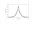
Figure 2: The perturbative short-distance function $f(t)$ for $m=5$ GeV and $\alpha_{s}=0.39$ (solid line) and the leading term in the delocalized multipole expansion of $f(t)$, $[\int dt^{\prime}f(t^{\prime})\tilde{e}_{0}^{\Omega}(t^{\prime})]$ for $\Omega=k^{2}/m$ (dashed line).

The characteristic width of $f$ is of order the energy $k^{2}/m\sim(m\alpha_{s}^{2})^{-1}\sim(mv^{2})^{-1}$. For the nonperturbative gluonic field strength correlator I use a lattice-inspired [7] model

$$\textstyle g(t)=12\,A_{0}\exp(-\sqrt{t^{2}+\lambda_{A}^{2}}/\lambda_{A}+1)$$

$$\textstyle A_{0}=0.04~{}\mbox{GeV}^{4}\,,\qquad\lambda_{A}^{-1}=0.7~{}\mbox{GeV}\,,$$ (20)

with a large-time behavior $\sim e^{-t/\Lambda_{A}}$. In this model the value of the gluon condensate is $\langle\frac{\alpha_{s}}{\pi}\,G_{\mu\nu}^{a}G_{\mu\nu}^{a}\rangle=\frac{6\,A_{0}}{\pi^{2}}=0.024\,\,\mbox{GeV}^{4}$.

				$\Omega=\infty$	$\Omega=\frac{k^{2}}{m}$
	$k^{2}/m$	$E^{np}$		$f_{n}g_{n}$	$f_{n}g_{n}$
$\alpha_{s}$	(GeV)	(MeV)	$n$	(MeV)	(MeV)
$0.39$	$0.338$	$24.8$	0	$38.6$	$24.2$
			2	$-65.7$	$-3.9$
			4	$832.7$	$12.1$
			6	$-35048.0$	$-43.1$
$0.15$	$1.750$	$0.245$	0	$0.258$	$0.249$
			2	$-0.016$	$-0.005$
			4	$0.008$	$0.003$
			6	$-0.012$	$-0.003$

Table 1: Nonperturbative corrections to the heavy quarkonium ground state level as described in the text.

In Tab. 1 the exact result and the first four terms of the resolution-dependent expansion of $E^{np}$ are shown for the quark masses $m=5$ (upper part) and $175$ GeV (lower part) and for $\Omega=\infty$ and $\Omega=k^{2}/m$. The strong coupling has been fixed by the relation $\alpha_{s}=\alpha_{s}(k)$. The numerical values of $f_{n}\,g_{n}$ have been determined from Eqs. (6,12). The series are all asymptotic. The local expansion is badly behaved for $m=5$ GeV because $k^{2}/m\mathrel{\raise 1.29167pt\hbox{$<$\kern-7.5pt\lower 4.30554pt\hbox{$\sim$}}}\lambda_{A}^{-1}$, and basically meaningless. For $m=175$ GeV, where $k^{2}/m>\lambda_{A}^{-1}$, the local expansion is good. For $\Omega=k^{2}/m$, however, the series is much better behaved for all quark masses. The size of the order $n$ term is about a factor $2^{-n}$ smaller than the order $n$ term in the local expansion. One also observes that even in the case $k^{2}/m<\lambda_{A}^{-1}$ the leading term in the delocalized expansion for $\Omega=k^{2}/m$ agrees with the exact result within a few percent. This feature is a general property of the delocalized expansion, and should apply to any quantity for which the local expansion in the ratio of two scales breaks down because the ratio is not sufficiently small.

4 RUNNING GLUON CONDENSATE FROM CHARMONIUM SUM RULES

The $\Omega$-dependent matrix elements are either determined from experimental data or from lattice measurements. In the following the $\Omega$-dependent (“running”) gluon condensate is extracted from charmonium sum rules which are based on moments [8]

$$\textstyle{\cal M}_{n}=\frac{1}{n!}(-\frac{d}{dQ^{2}})^{n}\Pi^{c}(Q^{2})|_{Q^{2}=0}$$ (21)

of the correlator of two charm quark vector currents $j_{\mu}\equiv\bar{c}\gamma_{\mu}c$. The moments can be determined theoretically in an expansion of the form [9]

$$\textstyle{\cal M}_{n}={\cal M}_{n}^{0}\{1+\mbox{[p. corr.]}+\delta^{(4)}_{n}\,\langle g^{2}G^{2}\rangle+\ldots\}\,,$$ (22)

while the experimental moments are obtained from a dispersion integral over the $c\bar{c}$ cross section in $e^{+}e^{-}$ annihilation. The Wilson coefficient of the gluon condensate, $\delta^{(4)}_{n}$, is $\Omega$-independent. We consider the ratio [8] $r_{n}\equiv\frac{{\cal M}_{n}}{{\cal M}_{n-1}}$ and extract the gluon condensate as a function of $n$. Since the relevant short-distance scale for the moment ${\cal M}_{n}$ is of order $m_{c}/n$, a proper choice for the resolution scale is $\Omega=2m_{c}/n$. Thus the dependence of the gluon condensate on $n$ can be interpreted as the dependence on $\Omega$. The results for the gluon condensate as a function of $n$ is shown in Fig. 3 for $n\leq 8$ and $\overline{m}_{c}(\overline{m}_{c})=1.23$ (white triangles), $1.24$ (black stars), $1.25$ (white squares) and $1.26$ GeV (black triangles). The area between the upper and lower symbols indicates the experimental and theoretical uncertainties.

Figure 3: The running gluon condensate as a function of $n$ when extracted from the ratio of charmonium moments $r_{n}$.

The running gluon condensate appears to be a decreasing function of $n$. The solid thick line is $\langle\frac{\alpha_{s}}{\pi}\,G^{2}\rangle(\Omega)$ obtained from the form of the gluon field strength correlator suggested from lattice computations [7] for $\Omega=(2.5\,\,\mbox{GeV})/n$ and the vacuum correlation length $\lambda_{A}^{-1}=0.7$ GeV. The qualitative agreement is encouraging but, the uncertainties of our extraction are still quite large. (See Ref. [3] for an analysis based on hadronic $\tau$ decay data.)

5 CONCLUSIONS

In this talk I discussed a generalization of the Wilson OPE based on nonlocal projections of gauge invariant correlation functions in a delocalized version of the multipole expansion for the perturbatively calculable coefficient functions. [3] This ”Delocalized Operator Expansion” (DOE) depends on an additional parameter $\Omega$, called ”resolution scale” which adjusts the width of the projection functions used for the expansion. The DOE has the same power counting as the OPE, but in general better convergence properties than the OPE. The DOE short-distance coefficients can be determined from the OPE Wilson coefficients at the same order in the expansion, whereas the DOE matrix elements correspond to an infinite sum of OPE matrix elements with additional covariant derivatives. I believe that the DOE can serve as a useful tool for situations where the OPE cannot be applied.

References

- [1]
- [2] M. A. Shifman, A. I. Vainshtein and V. I. Zakharov, Nucl. Phys. B 147, 385 (1979). Nucl. Phys. B 147, 448 (1979).
- [3] A. H. Hoang and R. Hofmann, arXiv:hep-ph/0206201.
- [4] H. G. Dosch and Y. A. Simonov, Phys. Lett. B 205, 339 (1988).
- [5] D. Gromes, Phys. Lett. B 115, 482 (1982); A. P. Bakulev and S. V. Mikhailov, Phys. Rev. D 65, 114511 (2002); P. Ball, V. M. Braun and H. G. Dosch, Phys. Rev. D 44, 3567 (1991); A. V. Radyushkin, Phys. Lett. B 271, 218 (1991).
- [6] M. B. Voloshin, Nucl. Phys. B 154, 365 (1979).
- [7] M. D’Elia, A. Di Giacomo and E. Meggiolaro, Phys. Lett. B 408, 315 (1997).
- [8] V. A. Novikov, L. B. Okun, M. A. Shifman, A. I. Vainshtein, M. B. Voloshin and V. I. Zakharov, Phys. Rev. Lett. 38, 626 (1977) [Erratum-ibid. 38, 791 (1977)]; Phys. Lett. B 67, 409 (1977).
- [9] S. N. Nikolaev and A. V. Radyushkin, Nucl. Phys. B 213, 285 (1983).