Abstract

We examine the use of two superbeam neutrino oscillation experiments with baselines $\mathrel{\raise 1.29167pt\hbox{$<$\kern-7.5pt\lower 4.30554pt\hbox{$\sim$}}}1000$ km to resolve parameter degeneracies inherent in the three-neutrino analysis of such experiments. We find that with appropriate choices of neutrino energies and baselines two experiments with different baselines can provide a much better determination of the neutrino mass ordering than a single experiment alone. Two baselines are especially beneficial when the mass scale for solar neutrino oscillations $\delta m^{2}_{\rm sol}$ is $\mathrel{\raise 1.29167pt\hbox{$>$\kern-7.5pt\lower 4.30554pt\hbox{$\sim$}}}5\times 10^{-5}$ eV². We also examine $CP$ violation sensitivity and the resolution of other parameter degeneracies. We find that the combined data of superbeam experiments with baselines of 295 and 900 km can provide sensitivity to both the neutrino mass ordering and $CP$ violation for $\sin^{2}2\theta_{13}$ down to 0.03 for $|\delta m^{2}_{\rm atm}|\simeq 3\times 10^{-3}$ eV². It would be advantageous to have a 10% determination of $|\delta m^{2}_{\rm atm}|$ before the beam energies and baselines are finalized, although if $|\delta m^{2}_{\rm atm}|$ is not that well known, the neutrino energies and baselines can be chosen to give fairly good sensitivity for a range of $|\delta m^{2}_{\rm atm}|$.

I Introduction

Atmospheric neutrino data from Super-Kamiokande provides strong evidence that $\nu_{\mu}$’s created in the atmosphere oscillate to $\nu_{\tau}$ with mass-squared difference $|\delta m^{2}_{\rm atm}|\sim 3\times 10^{-3}$ eV² and almost maximal amplitude [1]. Furthermore, the recent solar neutrino data from the Sudbury Neutrino Observatory (SNO) establishes that electron neutrinos change flavor as they travel from the Sun to the Earth: the neutral-current measurement is consistent with the solar neutrino flux predicted in the Standard Solar Model [2], while the charged-current measurement shows a depletion of the electron neutrino component relative to the total flux [3]. Global fits to solar neutrino data give a strong preference for the Large Mixing Angle (LMA) solution to the solar neutrino puzzle, with $\delta m^{2}_{\rm sol}\sim 5\times 10^{-5}$ eV² and amplitude close to 0.8 [3, 4].

The combined atmospheric and solar data may be explained by oscillations of three neutrinos, that are described by two mass-squared differences, three mixing angles and a $CP$ violating phase. The atmospheric and solar data roughly determine $\delta m^{2}_{\rm atm}$, $\delta m^{2}_{\rm sol}$ and the corresponding mixing angles. The LMA solar solution will be tested decisively (and $\delta m^{2}_{\rm sol}$ measured accurately) by the KamLAND reactor neutrino experiment [5, 6]. More precise measurements of the other oscillation parameters may be performed in long-baseline neutrino experiments. The low energy beam at MINOS [7] plus experiments with ICARUS [8] and OPERA [9] will allow an accurate determination of the atmospheric neutrino parameters and may provide the first evidence for oscillations of $\nu_{\mu}\to\nu_{e}$ at the atmospheric mass scale [10]. It will take a new generation of long-baseline experiments to further probe $\nu_{\mu}\to\nu_{e}$ appearance and to measure the leptonic $CP$ phase. Matter effects are the only means to determine sgn($\delta m^{2}_{\rm atm}$); once sgn($\delta m^{2}_{\rm atm}$) is known, the level of intrinsic $CP$ violation may be measured. Matter effects and intrinsic $CP$ violation both vanish in the limit that the mixing angle responsible for $\nu_{\mu}\to\nu_{e}$ oscillations of atmospheric neutrinos is zero.

It is now well-known that there are three two-fold parameter degeneracies that can occur in the measurement of the oscillation amplitude for $\nu_{\mu}\to\nu_{e}$ appearance, the ordering of the neutrino masses, and the $CP$ phase [11]. With only one $\nu$ and one $\bar{\nu}$ measurement, these degeneracies can lead to eight possible solutions for the oscillation parameters; in most cases, $CP$ violating ($CPV$) and $CP$ conserving ($CPC$) solutions can equally explain the same data. Studies have been done on how a superbeam [11, 12, 13, 14, 15, 16], neutrino factory [16, 17, 18], superbeam plus neutrino factory [19], or two superbeams with one at a very long baseline [20, 21] could be used to resolve one or more of these ambiguities.

In this paper we show that by combining the results of two superbeam experiments with different medium baselines, $\mathrel{\raise 1.29167pt\hbox{$<$\kern-7.5pt\lower 4.30554pt\hbox{$\sim$}}}1000$ km, the ambiguity associated with the sign of $\delta m^{2}_{\rm atm}$ can be resolved, even when it cannot be resolved by the two experiments taken separately. Furthermore, the ability to determine sgn($\delta m^{2}_{\rm atm}$) from the combined data is found to not be greatly sensitive to the size of $\delta m^{2}_{\rm sol}$, unlike the situation where data from only a single baseline is used. If both experiments are at or near the peak of the oscillation, a good compromise is obtained between the sensitivities for resolving sgn($\delta m^{2}_{\rm atm}$) and for establishing the existence of $CP$ violation. If $|\delta m^{2}_{\rm atm}|$ is not known accurately, the neutrino energies and baselines can be chosen to give fairly good sensitivity to the sign of $\delta m^{2}_{\rm atm}$ and to $CP$ violation for a range of $|\delta m^{2}_{\rm atm}|$.

The organization of our paper is as follows. In Sec. II we discuss the parameter degeneracies that can occur in the analysis of long-baseline oscillation data. In Sec. III we analyze how two long-baseline superbeam experiments can break degeneracies, determine the neutrino parameters, and establish the existence of $CP$ violation in the neutrino sector, if it is present. A summary is presented in Sec. IV.

II Parameter degeneracies

We work in the three-neutrino scenario using the parametrization for the neutrino mixing matrix of Ref. [11]. If we assume that $\nu_{3}$ is the neutrino eigenstate that is separated from the other two, then $\delta m^{2}_{31}=\delta m^{2}_{\rm atm}$ and the sign of $\delta m^{2}_{31}$ can be either positive or negative, corresponding to the mass of $\nu_{3}$ being either larger or smaller, respectively, than the other two masses. The solar oscillations are regulated by $\delta m^{2}_{21}=\delta m^{2}_{\rm sol}$, and thus $|\delta m^{2}_{21}|\ll|\delta m^{2}_{31}|$. If we accept the likely conclusion that the solar solution is LMA [3, 4], then $\delta m^{2}_{21}>0$ and we can restrict $\theta_{12}$ to the range $[0,\pi/4]$. It is known from reactor neutrino data that $\theta_{13}$ is small, with $\sin^{2}2\theta_{13}\leq 0.1$ at the 95% C.L. [22]. Thus a set of parameters that unambiguously spans the space is $\delta m^{2}_{31}$ (magnitude and sign), $\delta m^{2}_{21}$, $\sin^{2}2\theta_{12}$, $\sin\theta_{23}$, and $\sin^{2}2\theta_{13}$; only the $\theta_{23}$ angle can be below or above $\pi/4$.

For the oscillation probabilities for $\nu_{\mu}\to\nu_{e}$ and $\bar{\nu}_{\mu}\to\bar{\nu}_{e}$ we use approximate expressions given in Ref. [11], in which the probabilities are expanded in terms of the small parameters $\theta_{13}$ and $\delta m^{2}_{21}$ [23, 24], which reproduces well the exact oscillation probabilities for $E_{\nu}\mathrel{\raise 1.29167pt\hbox{$>$\kern-7.5pt\lower 4.30554pt\hbox{$\sim$}}}0.5$ GeV, $\theta_{13}\mathrel{\raise 1.29167pt\hbox{$<$\kern-7.5pt\lower 4.30554pt\hbox{$\sim$}}}9^{\circ}$, and $L\mathrel{\raise 1.29167pt\hbox{$<$\kern-7.5pt\lower 4.30554pt\hbox{$\sim$}}}4000$ km [11]. In all of our calculations we use the average electron density along the neutrino path, assuming the Preliminary Reference Earth Model [25]. Our calculational methods are described in Ref. [12].

We expect that $|\delta m^{2}_{31}|$ and $\sin^{2}2\theta_{23}$ will be measured to an accuracy of $\simeq 10$% at $3\sigma$ from $\nu_{\mu}\to\nu_{\mu}$ survival in long-baseline experiments [7, 8, 9, 10], while $\delta m^{2}_{21}$ will be measured to an accuracy of $\simeq 10$% at $2\sigma$ and $\sin^{2}2\theta_{12}$ will be measured to an accuracy of $\pm 0.1$ at $2\sigma$ in experiments with reactor neutrinos [6]. The remaining parameters ($\theta_{13}$, the $CP$ phase $\delta$, and the sign of $\delta m^{2}_{31}$) must be determined from long-baseline appearance experiments, principally using the modes $\nu_{\mu}\to\nu_{e}$ and $\bar{\nu}_{\mu}\to\bar{\nu}_{e}$ with conventional neutrino beams, or $\nu_{e}\to\nu_{\mu}$ and $\bar{\nu}_{e}\to\bar{\nu}_{\mu}$ at neutrino factories. However, there are three parameter degeneracies that can occur in such an analysis: (i) the ($\delta,\theta_{13}$) ambiguity [17], (ii) the sgn($\delta m^{2}_{31}$) ambiguity [13], and (iii) the ($\theta_{23},\pi/2-\theta_{23}$) ambiguity [11] (see Ref. [11] for a complete discussion of these three parameter degeneracies). In each degeneracy, two different sets of values for $\delta$ and $\theta_{13}$ can give the same measured rates for both $\nu$ and $\bar{\nu}$ appearance and disappearance. For each type of degeneracy the values of $\theta_{13}$ for the two equivalent solutions can be quite different, and the two values of $\delta$ may have different $CP$ properties, e.g., one can be $CP$ conserving and the other $CP$ violating.

A judicious choice of $L$ and $E_{\nu}$ can reduce the impact of the degeneracies. For example, if $L/E_{\nu}$ is chosen such that $\Delta\equiv|\delta m^{2}_{31}|L/(4E_{\nu})=\pi/2$ (the peak of the oscillation in vacuum), then the $\cos\delta$ terms in the average appearance probabilities vanish, even after matter effects are included [11]. Then since it is $\sin\delta$ that is being measured, the ($\delta,\theta_{13}$) ambiguity is reduced to a simple ($\delta,\pi-\delta$) ambiguity, $CPV$ solutions are no longer mixed with $CPC$ solutions, and $\theta_{13}$ is in principle determined (for a given sgn($\delta m^{2}_{31}$) and $\theta_{23}$). If $L$ is chosen to be long enough ($\mathrel{\raise 1.29167pt\hbox{$>$\kern-7.5pt\lower 4.30554pt\hbox{$\sim$}}}1000$ km), then the predictions for $\delta m^{2}_{31}>0$ and $\delta m^{2}_{31}<0$ no longer overlap if $\theta_{13}\mathrel{\raise 1.29167pt\hbox{$>$\kern-7.5pt\lower 4.30554pt\hbox{$\sim$}}}$ a few degrees, and the sgn($\delta m^{2}_{31}$) ambiguity is removed; our previous studies indicated that for $\delta m^{2}_{21}=5\times 10^{-5}$ eV² this happens at $L\mathrel{\raise 1.29167pt\hbox{$>$\kern-7.5pt\lower 4.30554pt\hbox{$\sim$}}}1300$ km if $\sin^{2}2\theta_{13}>0.01$ [11] (before experimental uncertainties are considered). However, the persistence of the sgn($\delta m^{2}_{31}$) ambiguity is highly dependent on the size of the solar oscillation mass scale, because large values of $\delta m^{2}_{21}$ cause the predictions for $\delta m^{2}_{31}>0$ and $\delta m^{2}_{31}<0$ to overlap much more severely than when $\delta m^{2}_{21}$ is smaller. Also, existing neutrino baselines are no longer than 735 km. In this paper we explore the possibility that two experiments with medium baselines ($\mathrel{\raise 1.29167pt\hbox{$<$\kern-7.5pt\lower 4.30554pt\hbox{$\sim$}}}1000$ km) can determine sgn($\delta m^{2}_{31}$), even when data from one of the baselines alone cannot. We then address the sensitivity for establishing $CP$ violation.

III Joint analysis of two superbeam experiments

A Description of the experiments and method

For our analysis we take one baseline to be 295 km, the distance for the proposed experiment from the Japan Hadron facility (JHF) to the Super-Kamiokande detector at Kamioka. For the neutrino spectrum of this experiment we use their $2^{\circ}$ off-axis beam with average neutrino energy of 0.7 GeV [26]. For the second experiment we assume an off-axis beam in which the beam axis points at a site 735 km from the source (appropriate for a beamline from NuMI at Fermilab to Soudan, or from CERN to Gran Sasso). For the off-axis spectra of the NuMI experiment we use the results presented in Ref. [27], which provides neutrino spectra for 39 different off-axis angles ranging from $0.32^{\circ}$ to $1.76^{\circ}$.

Using the off-axis components of the beam has the advantage of a lower background [15, 28, 29] due to reduced $\nu_{e}$ contamination and a smaller high-energy tail. Off-axis beams also offer flexibility in the choice of $L$ and $E_{\nu}$. For example, for a beam nominally aimed at a ground-level site a distance $L_{0}$ from the source, the distance to a ground-level detector with off-axis angle $\theta_{OA}$ can lie anywhere in the range

$$2R_{e}\sin(\theta-\theta_{OA})\leq L\leq 2R_{e}\sin(\theta+\theta_{OA})\,,$$ (1)

where $\sin\theta=L_{0}/(2R_{e})$, and $R_{e}=6371$ km is the radius of the Earth. Then for $L_{0}^{2}\ll R_{e}^{2}$ the possible range of distances for an off-axis detector at approximately ground level is

$$L_{0}-2R_{e}\theta_{OA}\mathrel{\raise 1.29167pt\hbox{$<$\kern-7.5pt\lower 4.30554pt\hbox{$\sim$}}}L\mathrel{\raise 1.29167pt\hbox{$<$\kern-7.5pt\lower 4.30554pt\hbox{$\sim$}}}L_{0}+2R_{e}\theta_{OA}\,.$$ (2)

The neutrino energy and neutrino flux $\Phi_{\nu}$ decrease with increasing off-axis angle as

$$E_{\nu}={0.43E_{\pi}\over 1+\gamma^{2}\theta_{OA}^{2}},~{}~{}~{}~{}~{}\Phi_{\nu}\propto{E_{\nu}^{2}\over L^{2}}\,,$$ (3)

where $\gamma=E_{\pi}/m_{\pi}$ is boost factor of the decaying pion. Thus a wide range of $L$ and $E_{\nu}$ can be achieved with a single fixed beam, although the event rate will drop with increasing off-axis angle because the flux decreases and the neutrino cross section is smaller at smaller $E_{\nu}$ (thereby putting a limit on the usable range of $L$ and $E_{\nu}$).

For the first experiment at $L_{1}=295$ km, we assume that the neutrino spectrum is chosen so that the $\cos\delta$ terms in the $\nu$ and $\bar{\nu}$ oscillation probabilities vanish (after averaging over the neutrino spectrum), using the best existing experimental value for $\delta m^{2}_{31}$. The JHF $2^{\circ}$ off-axis beam [30] satisfies this condition for $\delta m^{2}_{31}=3\times 10^{-3}$ eV². This spectrum choice reduces the ($\delta,\theta_{13}$) ambiguity to a simple ($\delta,\pi-\delta$) ambiguity, as described in Sec. II. For the second experiment we allow $L_{2}$ and $\theta_{OA}$ to vary within the restrictions of Eq. (2). This flexibility can be fully utilized if a deep underground site is not required; the short duration of the beam operation (an 8.6 $\mu$s pulse with a 1.9 s cycle time [31]) may enable a sufficient reduction in the cosmic ray neutrino background. We assume that the proton drivers at the neutrino sources have been upgraded from their initial designs (from 0.8 to 4.0 MW for JHF [30] and from 0.4 to 1.6 MW for FNAL [32]), so that they are both true neutrino superbeams. We assume two years running with neutrinos and six years with antineutrinos at JHF, and two years with neutrinos and five years with antineutrinos at FNAL; these running times give approximately equivalent numbers of charged-current events for neutrinos and antineutrinos at the two facilities, in the absence of oscillations. For detectors, we assume a 22.5 kt detector in the JHF beam (such as the current Super-K detector) and a 20 kt detector in the FNAL beam (which was proposed in Ref. [15]). Larger detectors such as Hyper-Kamiokande or UNO would allow shorter beam exposures or higher precision studies. In all of our calculations, we assume $|\delta m^{2}_{31}|=3\times 10^{-3}$ eV², $\theta_{23}=\pi/4$, $\delta m^{2}_{21}=5\times 10^{-5}$ eV², and $\sin^{2}2\theta_{12}=0.8$, unless noted otherwise.

We first consider the minimum value of $\sin^{2}2\theta_{13}$ for which the signal in the neutrino appearance channel can be seen above background at the $3\sigma$ level (the discovery reach), varying over a range of allowed values for $\theta_{OA}$ and $L_{2}$ in the second experiment. The discovery reach depends on the value of $\delta$ and the sign of $\delta m^{2}_{31}$; the best (when $\delta m^{2}_{31}>0$) and worst (when $\delta m^{2}_{31}<0$) cases in the $\nu$ channel (after varying over $\delta$) are shown in Fig. 1. In the $\bar{\nu}$ channel, the best case occurs for $\delta m^{2}_{31}<0$ and the worst for $\delta m^{2}_{31}>0$. In our calculations we assume a background that is 0.5% of the unoscillated charged-current rate (see Ref. [15]), and that the systematic error is 5% of the background. However, we note that our general conclusions are not significantly affected by reasonable changes in these experimental uncertainty assumptions. Detector positions where there is no $\cos\delta$ dependence in the rates are denoted by boxes. The best reach is $\sin^{2}2\theta_{13}\simeq 0.003$, which occurs for $\theta_{OA}\simeq 0.5$-$0.9^{\circ}$. In the worst case scenario the reach degrades to $\sin^{2}2\theta_{13}\simeq 0.01$.

The measurement of $P$ and $\bar{P}$ at $L_{1}$ allows a determination of $\sin^{2}2\theta_{13}$ and $\sin\delta$, modulo the possible uncertainty caused by the sign of $\delta m^{2}_{31}$, assuming for the moment that $\theta_{23}=\pi/4$, so there is no ($\theta_{23},\pi/2-\theta_{23}$) ambiguity. The question we next consider is whether an additional measurement of $P$ and $\bar{P}$ at $L_{2}$ can determine sgn($\delta m^{2}_{31}$), measure $CP$ violation, and distinguish $\delta$ from $\pi-\delta$. We define the $\chi^{2}$ of neutrino parameters ($\delta^{\prime},\theta_{13}^{\prime}$) relative to the parameters ($\delta,\theta_{13}$) as

$$\chi^{2}=\sum_{i}{(N_{i}-N_{i}^{\prime})^{2}\over(\delta N_{i})^{2}}\,,$$ (4)

where $N_{i}$ and $N_{i}^{\prime}$ are the event rates for the parameters ($\delta,\theta_{13}$) and ($\delta^{\prime},\theta_{13}^{\prime}$), respectively, $\delta N_{i}$ is the uncertainty in $N_{i}$, and $i$ is summed over the measurements being used in the analysis ($\nu$ and $\bar{\nu}$ at $L_{1}$ and $\nu$ and $\bar{\nu}$ at $L_{2}$). For $\delta N_{i}$ we assume that the statistical error for the signal plus background can be added in quadrature with the systematic error. For a two-parameter system ($\delta$ and $\theta_{13}$ unknown), two sets of parameters can be resolved at the $2\sigma$ ($3\sigma$) level if $\chi^{2}>6.17$ ($11.83$).

B Determining the sign of $\delta m^{2}_{31}$

To determine if measurements at $L_{1}$ and $L_{2}$ can distinguish one set of oscillation parameters with one sign of $\delta m^{2}_{31}$ from all other possible sets of oscillation parameters with the opposite sign of $\delta m^{2}_{31}$, we sample the ($\delta,\theta_{13}$) space for the opposite sgn($\delta m^{2}_{31}$) using a fine grid with $1^{\circ}$ spacing in $\delta$ and approximately 2% increments in $\sin^{2}2\theta_{13}$. If the $\chi^{2}$ between the original set of oscillation parameters and all of those with the opposite sgn($\delta m^{2}_{31}$) is greater than $6.17$ ($11.83$), then sgn($\delta m^{2}_{31}$) is distinguished at the $2\sigma$ ($3\sigma$) level for that parameter set.

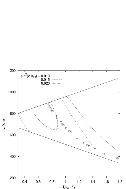
Figure 2 shows contours (in the space of possible $L_{2}$ and $\theta_{OA}$ for the second experiment) for the minimum value of $\sin^{2}2\theta_{13}$ (the $\sin^{2}2\theta_{13}$ reach) for distinguishing sgn($\delta m^{2}_{31}$) at the $3\sigma$ level when $\nu$ and $\bar{\nu}$ data from $L_{1}$ and $L_{2}$ are combined. As in Fig. 1, the boxes indicate the detector positions where the $\cos\delta$ terms in the average probabilities vanish. The best reach of about $\sin^{2}2\theta_{13}\simeq 0.03$ can be realized for $\theta_{OA}\simeq 0.7$-$1.0^{\circ}$ and $L_{2}$ values near the maximum allowed by Eq. 2 ($\simeq 875$-$950$ km). Table I shows the sensitivity for determining sgn($\delta m^{2}_{31}$) for different combinations of detector size and proton driver power in the two experiments. The table shows that once enough statistics are obtained at JHF (with a 22.5 kt detector and a 4 MW source), combined JHF and NuMI data significantly improve the $\sin^{2}2\theta_{13}$ reach for determining sgn($\delta m^{2}_{31}$) at $3\sigma$ (by nearly a factor of two compared to data from a 1.6 MW NuMI alone).

TABLE I.: $\sin^{2}2\theta_{13}$ reach for determining the sign of $\delta m^{2}_{31}$ at $3\sigma$ using $\nu$ and $\bar{\nu}$ data from JHF at 295 km and NuMI at $L_{2}$, for various detector sizes and proton driver powers. The approximate range of $\theta_{OA}$ that can obtain the reach shown is given in parentheses; $L_{2}\sim 900$ km in all cases.

	NuMI (20 kt)
JHF	0.4 MW	1.6 MW
	$\sin^{2}2\theta_{13}$ ($\theta_{OA}$)	$\sin^{2}2\theta_{13}$ ($\theta_{OA}$)
no JHF data	0.09 (0.7-1.0∘)	0.05 (0.8-1.0∘)
22.5 kt, 0.8 MW	0.07 (0.8-1.0∘)	0.04 (0.9-1.0∘)
22.5 kt, 4.0 MW	0.06 (0.7-1.0∘)	0.03 (0.7-1.0∘)
450 kt, 4.0 MW	0.05 (0.6-1.0∘)	0.02 (0.7-0.9∘)

The ability to distinguish the sign of $\delta m^{2}_{31}$ is greatly affected by the size of the solar mass scale $\delta m^{2}_{21}$, because the predictions for $\delta m^{2}_{31}>0$ and $\delta m^{2}_{31}<0$ overlap more for larger values of $\delta m^{2}_{21}$. In Fig. 3a we show the region in ($\delta,\sin^{2}2\theta_{13}$) space for which parameters with $\delta m^{2}_{31}>0$ can be distinguished from all parameters with $\delta m^{2}_{31}<0$ at the $3\sigma$ level for several possible values of $\delta m^{2}_{21}$, using combined data from $L_{1}=295$ km and $L_{2}=890$ km, with $\theta_{OA}=0.74^{\circ}$ for the second experiment. With this configuration the $\cos\delta$ terms in the average probabilities vanish for both experiments and nearly maximal reach for distinguishing sgn($\delta m^{2}_{31}$) is achieved. A similar plot using only data at $L_{2}=890$ km and $\theta_{OA}=0.74^{\circ}$ is shown in Fig. 3b. We do not show a corresponding plot for $L_{1}=295$ km because the shorter baseline severely inhibits the determination of sgn($\delta m^{2}_{31}$). A comparison of the two figures shows that for $\delta=270^{\circ}$ (where the $\delta m^{2}_{31}>0$ predictions have the least overlap with any of those for $\delta m^{2}_{31}<0$) the sensitivity to sgn($\delta m^{2}_{31}$) is not significantly improved by adding the data at $L_{1}$. However, at $\delta=90^{\circ}$ the ability to distinguish sgn($\delta m^{2}_{31}$) is much less affected by the value of $\delta m^{2}_{21}$ when the data at $L_{1}$ is included. With data only at $L_{2}$, sgn($\delta m^{2}_{31}$) can be determined for $\sin^{2}2\theta_{13}=0.1$ when $\delta=90^{\circ}$ only for $\delta m^{2}_{21}\mathrel{\raise 1.29167pt\hbox{$<$\kern-7.5pt\lower 4.30554pt\hbox{$\sim$}}}8\times 10^{-5}$eV², while with data at $L_{1}$ and $L_{2}$ it can be determined for $\sin^{2}2\theta_{13}$ as low as 0.04 for $\delta m^{2}_{21}$ as high as $2\times 10^{-4}$ eV². The corresponding results for $\delta m^{2}_{31}<0$ are approximately given by reflecting the curves in Fig. 3 about $\delta=180^{\circ}$.

We conclude that combining measurements of $\nu_{\mu}\to\nu_{e}$ and $\bar{\nu}_{\mu}\to\bar{\nu}_{e}$ from two superbeam experiments at different $L$ results in a much more sensitive test of the sign of $\delta m^{2}_{31}$ than one experiment alone, especially for larger values of the solar mass scale $\delta m^{2}_{21}$.

The ability to determine sgn($\delta m^{2}_{31}$) is also affected by the value of $\theta_{23}$. We found that the $\sin^{2}2\theta_{13}$ reach for determining sgn($\delta m^{2}_{31}$) at $3\sigma$ varied from 0.02 to 0.04 for $\sin^{2}2\theta_{23}=0.90$ (compared to 0.03 when $\theta_{23}=\pi/4$), depending on whether $\delta m^{2}_{31}$ is positive or negative, and whether $\theta_{23}<\pi/4$ or $\theta_{23}>\pi/4$. The sgn($\delta m^{2}_{31}$) sensitivities for different possibilities are shown in Table II.

TABLE II.: $\sin^{2}2\theta_{13}$ reach for determining the sign of $\delta m^{2}_{31}$ at $3\sigma$ using $\nu$ and $\bar{\nu}$ data from JHF at 295 km and NuMI at $L_{2}=890$ km with $\theta_{OA}=0.74^{\circ}$, for different combinations of sgn($\delta m^{2}_{31}$) and $\theta_{23}$, where $\sin^{2}2\theta_{23}=0.9$.

	$\sin^{2}2\theta_{13}$ reach for sgn($\delta m^{2}_{31}$)
sgn($\delta m^{2}_{31}$)	$\sin\theta_{23}=0.585$	$\sin\theta_{23}=0.811$
$+$	0.04	0.02
$-$	0.03	0.03

C Establishing the existence of $CP$ violation

An important goal of long-baseline experiments is to determine whether or not $CP$ is violated in the leptonic sector. In order to unambiguously establish the existence of $CP$ violation, one must be able to differentiate between ($\delta,\theta_{13}$) and all possible ($\delta^{\prime},\theta_{13}^{\prime}$), where $\delta^{\prime}=0^{\circ}$ or $180^{\circ}$ and $\theta_{13}^{\prime}$ can take on any value. For our $CP$ violation analysis we vary $\sin^{2}2\theta_{13}^{\prime}$ in 2% increments, as was done in the previous section when testing the sgn($\delta m^{2}_{13}$) sensitivity.

Figure 4 shows contours of $\sin^{2}2\theta_{13}$ reach for distinguishing $\delta=90^{\circ}$ from the $CP$ conserving values $\delta=0^{\circ}$ and $180^{\circ}$ at $3\sigma$ (with the same sgn($\delta m^{2}_{31}$)), plotted in the ($\theta_{OA},L_{2}$) plane, assuming $\nu$ and $\bar{\nu}$ data at both $L_{1}$ and $L_{2}$ are combined. The $CP$ reach in $\sin^{2}2\theta_{13}$ can go as low as 0.01 for $\theta_{OA}\simeq 0.5$ to $0.9^{\circ}$. Results for $\delta=270^{\circ}$ are similar to those for $\delta=90^{\circ}$.

Figure 5 shows the minimum value of $\sin^{2}2\theta_{13}$ for which $\delta$ can be distinguished from all $CP$ conserving parameter sets with $\delta=0^{\circ}$ and $180^{\circ}$, including those with the opposite sgn($\delta m^{2}_{31}$), at the $3\sigma$ level when $\theta_{OA}=0.74^{\circ}$ and $L_{2}=890$ km, for several different values of $\delta m^{2}_{21}$. Figure 5a shows the reaches if data from JHF and NuMI are combined, while Fig. 5b shows the reaches if data from NuMI only are used. For most values of $\delta$, when $\delta m^{2}_{21}$ is higher the $CP$ effect is increased, and hence $CP$ violation can be detected for smaller values of $\theta_{13}$. However, there is a possibility that a $CPV$ solution with one sgn($\delta m^{2}_{31}$) may not be as easily distinguishable from a $CPC$ solution with the opposite sgn($\delta m^{2}_{31}$); this occurs, e.g., in Fig. 5a for $\delta m^{2}_{21}=1\times 10^{-4}$ eV², where the predictions for ($\delta=45^{\circ}$ and $135^{\circ}$, $\delta m^{2}_{31}>0$) are close to those for ($\delta=0^{\circ}$ and $180^{\circ}$, $\delta m^{2}_{31}<0$); in this case the $CP$ reach for those values of $\delta$ is about the same for $\delta m^{2}_{21}=1\times 10^{-4}$ eV² and $\delta m^{2}_{21}=5\times 10^{-5}$ eV².

We note that if data from only JHF are used (and assuming $\sin^{2}2\theta_{13}\leq 0.1$) no value of the $CP$ phase can be distinguished at $3\sigma$ from the $CP$ conserving solutions when $\delta m^{2}_{21}\mathrel{\raise 1.29167pt\hbox{$<$\kern-7.5pt\lower 4.30554pt\hbox{$\sim$}}}8\times 10^{-5}$ eV², principally because the intrinsic $CP$ violation due to $\delta$ and the $CP$ violation due to matter have similar magnitudes and it is hard to disentangle the two effects. For larger values of $\delta m^{2}_{21}$, the intrinsic $CP$ effects are larger and $CP$ violation can be established; e.g., if $\delta m^{2}_{21}=1\times 10^{-4}$ ($2\times 10^{-4}$) eV², maximal $CP$ violation ($\delta=90^{\circ}$ or $270^{\circ}$) can be distinguished from $CP$ conservation at $3\sigma$ for $\sin^{2}2\theta_{13}\mathrel{\raise 1.29167pt\hbox{$>$\kern-7.5pt\lower 4.30554pt\hbox{$\sim$}}}0.006$ ($0.001$). Therefore, when $\delta m^{2}_{21}=1\times 10^{-4}$ eV², most of the $CP$ sensitivity of the combined JHF plus NuMI data results from the JHF data; for $\delta m^{2}_{21}=2\times 10^{-4}$ eV² the two experiments contribute about equally to the $CP$ sensitivity.

The boxes in Figs. 2 and 4 indicate the values of $L_{2}$ and $\theta_{OA}$ for which the $\cos\delta$ terms in the average probabilities vanish for the second experiment. As indicated in the figures, these detector positions are good for both distinguishing sgn($\delta m^{2}_{31}$) (see Fig. 2) and for establishing the existence of $CP$ violation (see Fig. 4), especially for larger values of $L_{2}$. A good compromise occurs at $\theta_{OA}\simeq 0.74^{\circ}$ with $L_{2}\simeq 890$ km. In Ref. [15] it was shown that similar values for $\theta_{OA}$ and $L_{2}$ using the NuMI off-axis beam gave a favorable figure-of-merit for the signal to background ratio; our analysis shows that such an off-axis angle and baseline is also very good for distinguishing sgn($\delta m^{2}_{31}$) and establishing $CP$ violation, when combined with superbeam data at $L_{1}=295$ km.

D Resolving the ($\delta,\pi-\delta$) ambiguity

If $L_{2}\simeq 890$ km and $\theta_{OA}\simeq 0.74^{\circ}$ are chosen for the location of the second experiment, as suggested in the previous section, then both the first and second experiments are effectively measuring $\sin\delta$, and it is impossible to resolve the ($\delta,\pi-\delta$) ambiguity. Different values of $L_{2}$ and $\theta_{OA}$ would be needed to distinguish $\delta$ from $\pi-\delta$.

Figure 6 shows contours (in the space of possible $L_{2}$ and $\theta_{OA}$) for the minimum value of $\sin^{2}2\theta_{13}$ needed to distinguish $\delta=0^{\circ}$ from $\delta=180^{\circ}$ at the $2\sigma$ level using $\nu$ and $\bar{\nu}$ data from $L_{1}$ and $L_{2}$ (it is not possible to distinguish $\delta=0^{\circ}$ from $\delta=180^{\circ}$ at the $3\sigma$ level for any value of $\sin^{2}2\theta_{13}\leq 0.1$). Two choices are possible: one with $\theta_{OA}\mathrel{\raise 1.29167pt\hbox{$<$\kern-7.5pt\lower 4.30554pt\hbox{$\sim$}}}0.3$-$0.5^{\circ}$ and $L_{2}\simeq 650$-$775$ km, and another near $\theta_{OA}\simeq 1.0^{\circ}$ with $L_{2}\simeq 950$ km. The former choice does not do well in distingishing sgn($\delta m^{2}_{31}$), while the latter choice is nearly optimal for sgn($\delta m^{2}_{31}$) sensitivity but significantly worse for $CP$ violation sensitivity. Thus the ability to also resolve the ($\delta,\pi-\delta$) ambiguity is rather poor, and comes at the expense of $CPV$ sensitivity.

E Resolving the ($\theta_{23},\pi/2-\theta_{23}$) ambiguity

If $\theta_{23}\neq\pi/4$, there is an additional ambiguity between $\theta_{23}$ and $\pi/2-\theta_{23}$. This ambiguity gives two solutions for $\sin^{2}2\theta_{13}$ whose ratio differs by a factor of approximately $\tan^{2}\theta_{23}$, which can be as large as 2 if $\sin^{2}2\theta_{23}=0.9$ [11]. Assuming $L_{1}=295$ km for the first experiment, we could not find any experimental configuration of $L_{2}$ and $\theta_{OA}$ for the second experiment that could resolve the ($\theta_{23},\pi/2-\theta_{23}$) ambiguity for $\sin^{2}2\theta_{13}\leq 0.1$ at even the $1\sigma$ level for the entire range of detector sizes and source powers listed in Table I. Therefore we conclude that superbeams are not effective at resolving the ($\theta_{23},\pi/2-\theta_{23}$) ambiguity using $\nu_{e}$ and $\bar{\nu}_{e}$ appearance data. Since the approximate oscillation probability for $\nu_{e}\to\nu_{\tau}$ is given by the interchanges $\sin\theta_{23}\leftrightarrow\cos\theta_{23}$ and $\delta\to-\delta$ in the expression for the $\nu_{\mu}\to\nu_{e}$ probability, a neutrino factory combined with detectors having tau neutrino detection capability provides a means for resolving the ($\theta_{23},\pi/2-\theta_{23}$) ambiguity [11]. Another possibility is to measure survival of $\bar{\nu}_{e}$’s from a reactor, which to leading order is sensitive to $\sin^{2}2\theta_{13}$ but not $\theta_{23}$ [33, 34].

F Dependence on $|\delta m^{2}_{31}|$

The foregoing analysis assumed $|\delta m^{2}_{31}|=3\times 10^{-3}$ eV². If the true value differs from this, then to sit on the peak (where the $\cos\delta$ terms vanish) requires tuning the beam energy and baseline according to the measured value of $|\delta m^{2}_{31}|$. JHF has the capability of varying the average $E_{\nu}$ from 0.4 GeV to 1.0 GeV, which would correspond to realizing the peak condition for $|\delta m^{2}_{31}|=1.6$-$4.0\times 10^{-3}$ eV² [30]. In principle, NuMI can vary both $L_{2}$ and $\theta_{OA}$ to be on the peak. If $|\delta m^{2}_{31}|<3\times 10^{-3}$ eV², then the best sensitivity to sgn($\delta m^{2}_{31}$) is obtained for larger $\theta_{OA}$ and longer distances (the larger angle makes $E_{\nu}$ smaller while the longer distance enhances the matter effect), and the sensitivity is reduced (since the matter effect is smaller for smaller $\delta m^{2}_{31}$). The $CP$ violation sensitivity is also reduced, although not as significantly. For larger values of $|\delta m^{2}_{31}|$ the sensitivity to sgn($\delta m^{2}_{31}$) is better, with $CP$ violation sensitivity about the same.

The tuning of the experiments to the peak (where the $\cos\delta$ terms in the average probabilities vanish) requires knowledge of $|\delta m^{2}_{31}|$ before the experimental design is finalized. The values of $|\delta m^{2}_{31}|$ and $\theta_{23}$ will be well-measured in the survival channel $\nu_{\mu}\to\nu_{\mu}$ measurements that would run somewhat before or concurrently with the appearance measurements being discussed here, but of course this information may not be available when the configurations for the off-axis experiments are chosen. If $|\delta m^{2}_{31}|$ is known to 10% at $3\sigma$ (the expected sensitivity of MINOS), then the sensitivities to sgn($\delta m^{2}_{31}$) and $CP$ violation are not greatly affected by baselines that are slightly off-peak. If the baselines and neutrino energies for the superbeam experiments must be chosen before a 10% measurement of $|\delta m^{2}_{31}|$ can be made, a loss of sensitivity to sgn($\delta m^{2}_{31}$) could result by not being on the peak. For example, if the experiments are designed for $|\delta m^{2}_{31}|=3\times 10^{-3}$ eV² but in fact $|\delta m^{2}_{31}|=2.5\times 10^{-3}$ eV², the $3\sigma$ sgn($\delta m^{2}_{31}$) reach is less ($\sin^{2}2\theta_{13}=0.04$, compared to 0.03 for $|\delta m^{2}_{31}|=3\times 10^{-3}$ eV²). If $|\delta m^{2}_{31}|$ is actually $2\times 10^{-3}$ eV², the $3\sigma$ sgn($\delta m^{2}_{31}$) reach extends only down to $\sin^{2}2\theta_{13}\simeq 0.075$, just a little below the CHOOZ bound.

Since the sgn($\delta m^{2}_{31}$) determination has the worst reach in $\sin^{2}2\theta_{13}$ (compared to the discovery reach and the $CPV$ sensitivity), and since not knowing sgn($\delta m^{2}_{31}$) can induce a $CPV/CPC$ ambiguity, the measurement of sgn($\delta m^{2}_{31}$) is crucial. If $|\delta m^{2}_{31}|$ is not known precisely, then the exact peak position is not known, and an off-axis angle and baseline should be chosen that will give a reasonable reach for sgn($\delta m^{2}_{31}$) over as much of the allowed range of $|\delta m^{2}_{31}|$ as possible. For example, $\theta_{OA}=0.85^{\circ}$-$0.90^{\circ}$ and $L\simeq 930$ km gives a sgn($\delta m^{2}_{31}$) reach that is fairly good for the range $|\delta m^{2}_{31}|=2\times 10^{-3}$ eV² to $4\times 10^{-3}$ eV². The reach for sgn($\delta m^{2}_{31}$) is farthest from optimal at the extremes ($\sin^{2}2\theta_{13}=0.06$ versus the best reach of 0.05 when $|\delta m^{2}_{31}|=2\times 10^{-3}$ eV² and 0.03 versus the best reach of 0.02 when $|\delta m^{2}_{31}|=4\times 10^{-3}$ eV²). But the $CPV$ reach remains at least as good as the sgn($\delta m^{2}_{31}$) reach for this range of $|\delta m^{2}_{31}|$.

IV Summary

We summarize the important points of our paper as follows:

1. Two superbeam experiments at different baselines, each measuring $\nu_{\mu}\to\nu_{e}$ and $\bar{\nu}_{\mu}\to\bar{\nu}_{e}$ appearance, are significantly better at resolving the sgn($\delta m^{2}_{31}$) ambiguity than one experiment alone. Using beams from a 4.0 MW JHF with a 22.5 kt detector $2^{\circ}$ off axis at 295 km and a 1.6 MW NuMI with a 20 kt detector $0.7$-$1.0^{\circ}$ off axis at $875$-$950$ km, sgn($\delta m^{2}_{31}$) can be determined for $\sin^{2}2\theta_{13}\mathrel{\raise 1.29167pt\hbox{$>$\kern-7.5pt\lower 4.30554pt\hbox{$\sim$}}}0.03$ if $\delta m^{2}_{31}=3\times 10^{-3}$ eV². Sensitivities for other beam powers and detector sizes are given in Table I.

2. For the most favorable cases, a higher value for the solar oscillation scale $\delta m^{2}_{21}$ does not greatly change the sensitivity to sgn($\delta m^{2}_{31}$) when $\nu$ and $\bar{\nu}$ data from two different baselines are combined (unlike the single baseline case, where the ability to determine sgn($\delta m^{2}_{31}$) is significantly worse for $\delta m^{2}_{21}\mathrel{\raise 1.29167pt\hbox{$>$\kern-7.5pt\lower 4.30554pt\hbox{$\sim$}}}5\times 10^{-5}$ eV²).

3. Running both experiments at the oscillation peaks, such that the $\cos\delta$ terms in the average probabilities vanish, provides good sensitivity to both sgn($\delta m^{2}_{31}$) and to $CP$ violation. On the other hand, the ability to resolve the ($\delta,\pi-\delta$) ambiguity is lost, and the ($\theta_{23},\pi/2-\theta_{23}$) ambiguity is not resolved for any experimental arrangement considered. However, the ($\delta,\pi-\delta$) and ($\theta_{23},\pi/2-\theta_{23}$) ambiguities do not substantially affect the ability to determine whether or not $CP$ is violated (although the latter ambiguity could affect the inferred value of $\theta_{13}$ by as much as a factor of 2).

4. Since running at or near the oscillation peaks is favorable, knowledge of $|\delta m^{2}_{31}|$ to about 10% (from MINOS) before these experiments are run would be advantageous. If $|\delta m^{2}_{31}|$ is not known that precisely in advance, then the detector off-axis angle and baseline can still be chosen to give fairly good (though not optimal) sensitivities to sgn($\delta m^{2}_{31}$) and $CP$ violation.

We conclude that superbeam experiments at different baselines may greatly improve the prospects for determining the neutrino mass ordering in the three-neutrino model. Since a good compromise between determining sgn($\delta m^{2}_{31}$) and establishing the existence of $CP$ violation is obtained when both experiments are tuned so that the $\cos\delta$ terms in the average probabilities approximately vanish, knowledge of $|\delta m^{2}_{31}|$ would be helpful for the optimal design for the experiments.

FIG. 1.: Contours of (a) best-case (when $\delta m^{2}_{31}>0$), and (b) worst-case (when $\delta m^{2}_{31}<0$), $\sin^{2}2\theta_{13}$ $3\sigma$ discovery reach in the ($\theta_{OA},L_{2}$) plane, for the $\nu$ channel at NuMI, where $\theta_{OA}$ is the off-axis angle and $L_{2}$ is the baseline of the NuMI detector. For the other neutrino parameters we assume $|\delta m^{2}_{31}|=3\times 10^{-3}$ eV², $\theta_{23}=\pi/4$, $\delta m^{2}_{21}=5\times 10^{-5}$ eV², and $\sin^{2}2\theta_{12}=0.8$. The boxes indicate detector positions for which the $\cos\delta$ terms in the average oscillation probabilities vanish. For the $\bar{\nu}$ channel the results are similar, except that the best case occurs for $\delta m^{2}_{31}<0$ and the worst case for $\delta m^{2}_{31}>0$.

FIG. 2.: Contours of $\sin^{2}2\theta_{13}$ reach for resolving the sign of $\delta m^{2}_{31}$ at the $3\sigma$ level in the ($\theta_{OA},L_{2}$) plane when data from JHF and NuMI are used. The JHF detector is assumed to have baseline $L_{1}=295$ km. Other parameters and notation are the same as in Fig. 1.

FIG. 3.: Minimum value of $\sin^{2}2\theta_{13}$ for which sgn($\delta m^{2}_{31}$) may be determined at $3\sigma$, assuming the true solution has $\delta m^{2}_{31}>0$, using $\nu$ and $\bar{\nu}$ data from (a) JHF with $L_{1}=295$ km and NuMI with $L_{2}=890$ km, and (b) only NuMI with $L_{2}=890$ km, for several values of $\delta m^{2}_{21}$ (in eV²). The off-axis angle for the NuMI detector is $\theta_{OA}=0.74^{\circ}$. Other parameters are the same as in Fig. 1. Results for $\delta m^{2}_{31}<0$ are approximately given by reflecting the curves about $\delta=180^{\circ}$.

FIG. 4.: Contours of $\sin^{2}2\theta_{13}$ reach for distinguishing $\delta=90^{\circ}$ from the $CP$ conserving values $\delta=0^{\circ}$ and $180^{\circ}$ at $3\sigma$ (for the same sgn($\delta m^{2}_{31}$)), plotted in the ($\theta_{OA},L_{2}$) plane, when data from JHF and NuMI are combined. Other parameters and notation are the same as in Fig. 1. Results for $\delta=270^{\circ}$ are similar to those for $\delta=90^{\circ}$.

FIG. 5.: Minimum value of $\sin^{2}2\theta_{13}$ versus $CP$ phase $\delta$ for which $\delta$ can be distinguished from the $CP$ conserving values $\delta=0^{\circ}$ and $180^{\circ}$ (with either sign of $\delta m^{2}_{31}$) at the $3\sigma$ level when (a) data from JHF and NuMI are combined, and (b) data from NuMI only are used. The baseline for JHF is $L_{1}=295$ km, while for NuMI $L_{2}=890$ km and $\theta_{OA}=0.74^{\circ}$. The curves are plotted for several values of the solar mass scale $\delta m^{2}_{21}$ (in eV²). Other parameters are the same as in Fig. 1.

FIG. 6.: Contours of $\sin^{2}2\theta_{13}$ reach for distinguishing $\delta=0^{\circ}$ from $\delta=180^{\circ}$ (the $(\delta,\pi-\delta)$ ambiguity) at the $2\sigma$ level, plotted in the ($\theta_{OA},L_{2}$) plane, when data from JHF and NuMI are combined. Other parameters and notation are the same as in Fig. 1.

REFERENCES

- [1] T. Toshito [Super-Kamiokande Collaboration], arXiv:hep-ex/0105023.
- [2] J. N. Bahcall, M. H. Pinsonneault and S. Basu, Astrophys. J. 555, 990 (2001) [arXiv:astro-ph/0010346].
- [3] Q. R. Ahmad et al. [SNO Collaboration], arXiv:nucl-ex/0204008, arXiv:nucl-ex/0204009.
- [4] V. Barger, D. Marfatia, K. Whisnant, and B.P. Wood, Phys. Lett. B 537, 179 (2002) [arXiv:hep-ph/0204253]; A. Bandyopadhyay, S. Choubey, S. Goswami and D.P. Roy, arXiv:hep-ph/0204286; J. N. Bahcall, M. C. Gonzalez-Garcia and C. Pena-Garay, arXiv:hep-ph/0204314; P. Aliani, V. Antonelli, R. Ferrari, M. Picariello, and E. Torrente-Lujan, arXiv:hep-ph/0205053; P.C. de Holanda and A. Yu. Smirnov, arXiv:hep-ph/0205241; A. Strumia, C. Cattadori, N. Ferrari and F. Vissani, Phys. Lett. B 541, 327 (2002) [arXiv:hep-ph/0205261]; G. L. Fogli, E. Lisi, A. Marrone, D. Montanino and A. Palazzo, Phys. Rev. D 66, 053010 (2002) [arXiv:hep-ph/0206162]; M. Maltoni, T. Schwetz, M. A. Tortola and J. W. Valle, arXiv:hep-ph/0207227.
- [5] P. Alivisatos et al., STANFORD-HEP-98-03.
- [6] V. Barger, D. Marfatia and B. P. Wood, Phys. Lett. B 498, 53 (2001) [arXiv:hep-ph/0011251].
- [7] MINOS Collaboration, Fermilab Report No. NuMI-L-375 (1998).
- [8] A. Rubbia for the ICARUS Collaboration, talk given at Skandinavian NeutrinO Workshop (SNOW), Uppsala, Sweden, February (2001), which are available at http://pcnometh4.cern.ch/publicpdf.html .
- [9] OPERA Collaboration, CERN/SPSC 2000-028, SPSC/P318, LNGS P25/2000, July, 2000.
- [10] V. Barger, A. M. Gago, D. Marfatia, W. J. Teves, B. P. Wood and R. Z. Funchal, Phys. Rev. D 65, 053016 (2002) [arXiv:hep-ph/0110393].
- [11] V. Barger, D. Marfatia, and K. Whisnant, Phys. Rev. D 65, 073023 (2002) [arXiv:hep-ph/0112119].
- [12] V. Barger, D. Marfatia, and K. Whisnant, Phys. Rev. D 66, 053007 (2002) [arXiv:hep-ph/0206038].
- [13] H. Minakata and H. Nunokawa, JHEP 0110, 001 (2001) [arXiv:hep-ph/0108085]; V. D. Barger, D. Marfatia and K. Whisnant, in Proc. of the APS/DPF/DPB Summer Study on the Future of Particle Physics (Snowmass 2001) ed. N. Graf, arXiv:hep-ph/0108090.
- [14] T. Kajita, H. Minakata, and H. Nunokawa, arXiv:hep-ph/0112345.
- [15] G. Barenboim, A. de Gouvea, M. Szleper, and M. Velasco, arXiv:hep-ph/0204208.
- [16] P. Huber, M. Lindner, and W. Winter, arXiv:hep-ph/0204352.
- [17] J. Burguet-Castell, M. B. Gavela, J. J. Gomez-Cadenas, P. Hernandez and O. Mena, Nucl. Phys. B 608, 301 (2001) [arXiv:hep-ph/0103258].
- [18] M. Freund, P. Huber and M. Lindner, Nucl. Phys. B 615, 331 (2001) [arXiv:hep-ph/0105071]; J. Pinney and O. Yasuda, Phys. Rev. D 64, 093008 (2001) [arXiv:hep-ph/0105087]; A. Donini, D. Meloni and P. Magliozzi, arXiv:hep-ph/0206034.
- [19] J. Burguet-Castell, M. B. Gavela, J. J. Gomez-Cadenas, P. Hernandez and O. Mena, arXiv:hep-ph/0207080.
- [20] Y.F. Wang, K. Whisnant, Jinmin Yang and Bing-Lin Young, Phys. Rev. D 65, 073021 (2002) [arXiv:hep-ph/0111317]; K. Whisnant, Jinmin Yang and Bing-Lin Young, arXiv:hep-ph/0208193.
- [21] M. Aoki, K. Hagiwara, Y. Hayoto, T. Kobayashi, T. Nakaya, K. Nishikawa, and N. Okamura, arXiv:hep-ph/0112338.
- [22] M. Apollonio et al. [CHOOZ Collaboration], Phys. Lett. B 466, 415 (1999) [arXiv:hep-ex/9907037].
- [23] A. Cervera et al., Nucl. Phys. B 579, 17 (2000) [Erratum-ibid. B 593, 731 (2000)] [arXiv:hep-ph/0002108].
- [24] M. Freund, Phys. Rev. D 64, 053003 (2001) [arXiv:hep-ph/0103300].
- [25] A. Dziewonski and D. Anderson, Phys. Earth Planet. Inter. 25, 297 (1981).
- [26] The expected JHF off-axis spectra with a 0.8 MW proton driver are available at http://neutrino.kek.jp/~kobayashi/50gev/beam/0101/ .
- [27] Anticipated neutrino spectra from a 0.4 MW NuMI for a range of off-axis angles can be found at http://www-numi.fnal.gov/fnal_minos/new_initiatives/beam/beam.html .
- [28] D. Beavis et al., E889 Collaboration, BNL preprint BNL-52459, April 1995.
- [29] A. Para and M. Szleper, arXiv:hep-ex/0110032.
- [30] Y. Itow et al., arXiv:hep-ex/0106019.
- [31] J. Hylen et al., “Conceptual design for the technical components of the neutrino beam for the main injector (NuMI),” Fermilab-TM-2018, September 1997.
- [32] “The proton driver study,” ed. by W. Chou, Fermilab-TM-2136.
- [33] G. Barenboim and A. de Gouvea, arXiv:hep-ph/0209117.
- [34] H. Minakata, H. Sugiyama, O. Yasuda, K. Inoue and F. Suekane, arXiv:hep-ph/0211111.