High-Multiplicity $pA$ collisions and the small-$x$ effective action

Abstract

I discuss the $p_{t}$ distributions for high-multiplicity events originating from semi-classical variation of the gluon density of the proton. The multiplicity distribution measures the curvature of the effective action for the small-$x$ gluon fields. For $pA$ collisions at the RHIC and LHC colliders, semi-classically the multiplicity distribution reflects the distribution of saturation momenta of the proton but not that of the nucleus. The average transverse momentum in the central region grows with $dN/dy$, while the $p_{t}$ distribution of leading hadrons in the proton fragmentation region should depend less on the multiplicity in the central region.

High-energy hadronic scattering requires understanding of the non-abelian gauge fields of hadrons at small $x$, which is the fractional light-cone energy carried by the quanta of the fields. At very high energy, $\log 1/x\gg 1$, the gluon fields in a hadron become very strong, corresponding to high gluon density. This is where one expects that cross sections become comparable to the geometric size of the hadron and where the unitarity limit is reached. A perturbative QCD based mechanism for unitarization of cross sections is provided by gluon saturation effects [1]. A semi-classical approach to gluon saturation and QCD at high energy was developed in [2, 3, 4, 5, 6, 7, 8] and will be applied here to high energy proton-nucleus collisions.

Large nuclei facilitate the study of gluon saturation effects because the gluon density per unit transverse area is larger than in a proton. The scale associated with the high gluon density, the saturation scale $Q_{s}$, grows with energy and atomic number $A$. At a resolution less than $Q_{s}^{2}$, the color field carries large occupation numbers, of order of the inverse QCD coupling constant, $1/\alpha_{s}$. Thus, the nuclear wave function at $Q^{2}<Q_{s}^{2}$ resembles a Bose “condensate”. The local color charge density in the transverse plane is a stochastic variable which eventually has to be averaged over, see below. Also, by Lorentz time dilation the large $x$ gluons evolve slowly and so for the small-$x$ gluons they appear as a “frozen” source near the light cone. Therefore, the high gluon density state of QCD at $Q^{2}\mathrel{\lower 3.87495pt\hbox{$\stackrel{{\scriptstyle\displaystyle<}}{{\sim}}$}}Q_{s}^{2}$ is called a “Color Glass Condensate” [6].

The small-$x$ gluon fields of hadrons or nuclei can be treated semi-classically because the occupation numbers parametrically are of order $1/\alpha_{s}\gg 1$. One can integrate out the fields at large $x$ whose dynamics is “frozen”, thereby generating an effective action for the small-$x$ gluons [2, 3, 4, 5, 6, 7, 8],

$$S[\rho]=\int dy\,d^{2}x_{t}\,V[\rho]~{},$$ (1)

with $y$ being the rapidity. The large-$x$ gluons effectively act as a source of color charge in the Yang-Mills equations of motion for the small-$x$ fields; $\rho$ denotes the color charge density per unit transverse area $d^{2}x_{t}$, and rapidity $dy$. This is a stochastic variable which eventually has to be integrated over,

$$\langle O\rangle=\int{\cal D}\rho\,\exp(-S[\rho])\,O[\rho]~{},$$ (2)

where $O[\rho]$ denotes some observable which is a functional of $\rho$. In their original papers [2], McLerran and Venugopalan suggested the simplest possible effective potential

$$V_{2}[\rho;\mu^{2}]=\frac{{\rm tr}\,\rho^{2}}{\mu^{2}}~{}.$$ (3)

This is the lowest-dimensional operator. In (3), $\mu^{2}$ is a real number, and physically is simply the mean square fluctuation of the density of “hard”, large-$x$ gluons in the source. It determines the curvature of the effective potential at the minimum.

FIG. 1.: Double-well potential for the color charge density per unit area.

In principle, one might try other choices for the effective potential $V[\rho]$, c.f. [9, 10], as for example the double well potential depicted in Fig. 1, which looks just like the effective potential for a first-order phase transition in thermal $SU(3)$ gauge theory near $T_{c}$ [11]. The curvature of the potential in the first well at $\rho_{1}$ is $1/\mu_{1}$, and that in the second well is $1/\mu_{2}$. Semiclassically, one considers only small fluctuations about the states which minimize the action. Thus, for this potential the averaging over $\rho$ from eq. (2) turns into

$$\sum\limits_{i=1,2}w_{i}\int{\cal D}\rho\,\exp\left(-\int dy\,d^{2}x_{t}\,V_{2}[\rho-\rho_{i};\mu_{i}^{2}]\right)\,O[\rho]~{}.$$ (4)

The probabilities for the configurations $\rho_{1}$ or $\rho_{2}$ are determined by the classical action:

$$w_{i}=\frac{\exp(-S[\rho_{i}])}{\exp(-S[\rho_{1}])+\exp(-S[\rho_{2}])}~{}.$$ (5)

Note that if the effective potential is quadratic for small fluctuations about each of its minima, renormalization-group evolution presumably preserves that functional form [3, 4, 5, 6]. That is, imposing the potential from Fig. 1 as the initial condition (at small rapidity), it will keep its shape at larger rapidity, and the ratio of the curvatures at the two minima stays the same.

One can evidently generalize the above to effective potentials with several classical minima. One could also imagine that there is a continuum of nearly degenerate states near a classical minimum. For example, at a tricritical point the lowest-dimensional operator appearing in the action is $\sim{\rm tr}\rho^{6}$. The state of lowest action is that for $\rho=0$ but the potential about that classical state is flat, and so states in its vicinity are nearly degenerate. This type of potential might not be preserved by the RG evolution in rapidity, though.

The distribution $w(\mu^{2})$ of correlation lengths determines the multiplicity distribution in hadronic collisions. Here, I do not attempt to compute that distribution. Rather, given a nonvanishing probability for a class of events with higher multiplicity $dN/dy$ than the average, I discuss the origin of such events and how the $p_{t}$ distribution in that class of events is different from the average. Nevertheless, it will be very interesting of course to analyze the multiplicity distribution experimentally; for example, at a tricritical point events with larger than average multiplicity could be due to semi-classical fluctuations of the color charge density. A potential with several discrete local minima as in Fig. 1 would lead to multiple peaks in the multiplicity distribution, unless the curvature radii of the potential are the same. For finite temperatures, the effect of a second local minimum in the effective potential on multiplicity and momentum distributions of produced particles has been discussed previously using the hydrodynamical model [12].

Henceforth, I consider “$pA$” collisions, i.e. collisions of a dilute projectile with a dense target. For simplicity, $\mu^{2}$ for the nucleus is chosen to be constant over the transverse plane. For large nuclei ($A\simeq 200$) this should not be a bad approximation. Realistic transverse density distributions can be treated numerically [13]. Moreover, experimental triggers in the fragmentation region of the nucleus, for example a trigger on the number of knocked-out neutrons, could improve the selection of central events. This might be particularly important for composite projectiles (small nuclei) to ensure that all nucleons have hit the large nuclear target.

For “$pA$” collisions an analytical solution for the radiation field in the forward light-cone can be found to first order in the coupling to the proton field, but to all orders in the density of the nucleus (see below). In principle, there is a contribution to large multiplicity events from coupling the radiation field to second (and higher) order to the proton source, down by additional powers of $\alpha_{s}$. That corresponds to attaching additional non-collinear hard gluon lines to the proton source (collinear emissions are already resummed in eq. (22) through the DGLAP logarithm), see e.g. [14]. As already mentioned above, for the simplest quadratic effective potential this is in fact the only contribution to large-multiplicity events since the effective potential exhibits only one classical minimum (i.e. the distribution of saturation momenta is a $\delta$-function). In general, if the potential starts out with some higher-dimensional operator, the distribution of saturation momenta is less sharply peaked, or it exhibits several peaks as for the double well potential above, and so high-multiplicity events can occur semi-classically. Their contribution dominates when $\exp(-\Delta S[\rho])>\alpha_{s}$, where $\Delta S[\rho]$ is the action relative to that at the global minimum. This condition determines the “cut-off” of the semi-classical multiplicity distribution.

In light-cone gauge, the classical fields of the sources before the collision, which occurs at the tip of the light-cone, are given by the single-hadron (nucleus) solutions

$$A^{\pm}_{1,2} = 0~{},$$ (6)

$$A^{i}_{1,2} = \frac{i}{g}U_{1,2}(x_{\perp})\,\partial^{i}\,U^{\dagger}_{1,2}(x_{\perp})~{}.$$ (7)

The $U_{1,2}$’s are rotation matrices in color space,

$$U_{1,2}(x_{t})=\exp\left(-ig\Phi_{1,2}(x_{t})\right)~{}.$$ (8)

The gauge potentials $\Phi_{1,2}$ satisfy the two-dimensional Poisson equation

$$-\nabla^{2}\Phi_{1,2}(x_{t})=g\,\rho_{1,2}(x_{t})~{}.$$ (9)

The average over the color charge density configurations $\rho_{1}$ and $\rho_{2}$ with a Gaussian weight as in eq. (2) thus corresponds to an average over the rotations in color space, $U_{1,2}$.

The fields (7) serve as the initial conditions for solving the Yang-Mills equations of motion in the forward light cone; they were solved in [15] for the case of asymmetric collisions where the classical field of one of the colliding sources is much stronger than that of the other source. Chosing the gauge $x^{+}A^{-}+x^{-}A^{+}=0$, the radiation field in the forward light cone region is given by

$$A^{i}(\tau,x_{t}) = U(x_{t})\left(\beta^{i}(\tau,x_{t})+\frac{i}{g}\partial^{i}\right)U^{\dagger}(x_{t})~{},$$ (10)

$$A^{\pm}(\tau,x_{t}) = \pm x^{\pm}\,U(x_{t})\,\beta(\tau,x_{t})\,U^{\dagger}(x_{t})~{}.$$ (11)

Here, $\tau=\sqrt{2x^{+}x^{-}}$ denotes proper time and $x_{t}$ is the transverse coordinate. The $U$’s are rotation matrices in color space, to be specified shortly. At asymptotic times, $\tau\to\infty$, the fields $\beta$ and $\beta^{i}$ are given by superpositions of plane wave solutions,

$$\beta(\tau\to\infty,x_{t}) =$$ (13)

$$\int\frac{d^{2}p_{t}}{(2\pi)^{2}}\frac{1}{\sqrt{2\omega\tau^{3}}}\left\{a_{1}(p_{t})e^{ip_{t}\cdot x_{t}-i\omega\tau}+c.c.\right\}~{},$$

$$\beta^{i}(\tau\to\infty,x_{t}) =$$ (15)

$$\int\frac{d^{2}p_{t}}{(2\pi)^{2}}\frac{1}{\sqrt{2\omega\tau}}\frac{\epsilon^{il}p_{t}^{l}}{\omega}\left\{a_{2}(p_{t})e^{ip_{t}\cdot x_{t}-i\omega\tau}+c.c.\right\}~{}.$$

The number distribution of produced gluons at rapidity $y$ and transverse momentum $p_{t}$ is given by

$$\frac{dN}{d^{2}p_{t}\,dy}=\frac{2}{(2\pi)^{2}}{\rm tr}~{}\left<\left|a_{1}(p_{t})\right|^{2}+\left|a_{2}(p_{t})\right|^{2}\right>~{}.$$ (16)

For $pA$ collisions, the $U$’s appearing in eq. (11) are just the $U_{2}$’s from eq. (7); that is, to leading order in the weak field, the plane waves in the forward light cone are just gauge rotated by the strong field.

The squared amplitudes now have to be averaged over the density configurations. The radiation number distribution (16) depends on the integrated color charge densities of the sources,

$$\chi_{p}(y) = \int\limits_{y}^{y_{p}}dy^{\prime}\,\mu^{2}_{p}(y^{\prime})~{},$$ (17)

$$\chi_{A}(y) = \int\limits_{y_{A}}^{y}dy^{\prime}\,\mu^{2}_{A}(y^{\prime})~{},$$ (18)

where $y_{p}=-y_{A}$ denote the beam rapidities. Due to the nuclear enhancement, in the central region $\chi_{A}\gg\chi_{p}$. Up to some proportionality constant which is of no relevance here, the integrated color charge densities $\chi_{p,A}$ times $g^{4}$ equal the saturation scales $Q_{p,A}^{2}$ of the sources.

A high-resolution probe with $p_{t}\gg Q_{A}(y)$ resolves the gluons in the target nucleus, i.e. it appears dilute at that scale, while a low-resolution source with $p_{t}\mathrel{\lower 3.87495pt\hbox{$\stackrel{{\scriptstyle\displaystyle<}}{{\sim}}$}}Q_{A}(y)$ sees a dense, nearly “black” target without structure (see the expressions for the gluon-nucleus cross section in the various regimes in [16]). In particular, since $Q_{A}(y)\gg Q_{p}(y)$ at central rapidity, for gluons produced with transverse momenta $Q_{p}(y)\mathrel{\lower 3.87495pt\hbox{$\stackrel{{\scriptstyle\displaystyle<}}{{\sim}}$}}p_{t}\mathrel{\lower 3.87495pt\hbox{$\stackrel{{\scriptstyle\displaystyle<}}{{\sim}}$}}Q_{A}(y)$ the proton projectile is dilute while the nuclear target is dense. Performing the integrals over color charge density configurations with a quadratic potential for fixed saturation momenta $Q_{A}$ and $Q_{p}$, the transverse momentum distributions in the two regimes are given by [15]

$$\frac{dN}{d^{2}b\,d^{2}p_{t}\,dy} \sim \frac{1}{g^{2}}\frac{Q_{A}^{2}(y)\,Q_{p}^{2}(y)}{p_{t}^{4}}\log\frac{p_{t}^{2}}{Q_{A}^{2}(y)}$$ (20)

$$\hskip 99.58464pt(p_{t}>Q_{A})$$

$$\frac{dN}{d^{2}b\,d^{2}p_{t}\,dy} \sim \frac{1}{g^{2}}\,\frac{Q_{p}^{2}(y)}{p_{t}^{2}}\log\frac{p_{t}^{2}}{Q_{p}^{2}(y)}$$ (22)

$$\hskip 85.35826pt(Q_{p}\mathrel{\lower 3.87495pt\hbox{$\stackrel{{\scriptstyle\displaystyle<}}{{\sim}}$}}p_{t}\mathrel{\lower 3.87495pt\hbox{$\stackrel{{\scriptstyle\displaystyle<}}{{\sim}}$}}Q_{A})~{}.$$

Again, some proportionality constants which are inessential for the present discussion have been dropped (see [15]). The logarithm in eq. (22) arises from resumming collinear gluon emissions from the proton source at the scale $p_{t}^{2}$ [16], i.e. from DGLAP evolution. For $Q_{A}\gg Q_{p}\simeq\Lambda_{\rm QCD}$ the dominant contribution to the multiplicity density per unit rapidity is from the region (22),

$$\frac{dN}{d^{2}b\,dy}\sim\frac{1}{g^{2}}\,Q_{p}^{2}(y)\,\log^{2}\frac{Q_{A}^{2}(y)}{Q_{p}^{2}(y)}~{}.$$ (23)

The contribution from the high-$p_{t}$ region (20) is

$$\frac{dN}{d^{2}b\,dy}\sim\frac{1}{g^{2}}\,Q_{p}^{2}(y)~{}.$$ (24)

Thus, fluctuations in the $p_{t}$-integrated multiplicity per unit rapidity, $dN/dy$, should be dominated by fluctuations of the saturation momentum of the proton. Fluctuations of $Q_{A}$ do occur but their effect on $dN/dy$ is logarithmically suppressed, and so the two quantities are approximately uncorrelated. This can be seen also from the fact that for a dense nuclear target, the gluon-nucleus [16] and the quark-nucleus [18] cross sections are essentially given by the nuclear area $\pi R_{A}^{2}$, which does not vary; once the target has reached the “black-body limit”, cross sections are geometrical. Rather, high-multiplicity events originate from larger than average density of partons in the dilute projectile proton. Note that fluctuations of the inelastic $pA$ cross section have been considered previously, e.g. ref. [19]. What is new here is that the distribution of inelastic cross sections is related to the distribution of correlation lengths exhibited by the effective action (1), and that the transverse momentum distributions of produced particles changes systematically with multiplicity, see below.

Thus, to first approximation an average over many events within one event class (which is defined by $dN/dy$) corresponds to an average over $Q_{A}$ at fixed $Q_{p}$:

$$\frac{dN}{d^{2}p_{t}\,dy}(\mu^{2}_{p}) = \int d\mu^{2}_{A}\,w(\mu^{2}_{A})\int{\cal D}\rho_{p}\,e^{-S[\rho_{p},\mu^{2}_{p}]}$$ (26)

$$\times\int{\cal D}\rho_{A}\,e^{-S[\rho_{A},\mu^{2}_{A}]}\frac{2}{(2\pi)^{2}}\,{\rm tr}\,\left(|a_{1}|^{2}+|a_{2}|^{2}\right)$$

$$= \int{\cal D}\rho_{p}\,e^{-S[\rho_{p},\mu^{2}_{p}]}\int{\cal D}\rho_{A}\,e^{-S[\rho_{A},\overline{\mu^{2}_{A}}]}$$ (28)

$$\quad\times\frac{2}{(2\pi)^{2}}\,{\rm tr}\,\left(|a_{1}|^{2}+|a_{2}|^{2}\right)~{}.$$

Note the difference to fluctuations of the multiplicity at high transverse momentum above some (large) fixed cutoff $p_{0}$. The integral of the distribution (20) from binary hard scatterings over $p_{t}>p_{0}$ (with $p_{0}>Q_{A}$) is equally sensitive to fluctuations of both the projectile density as well as the target density [14].

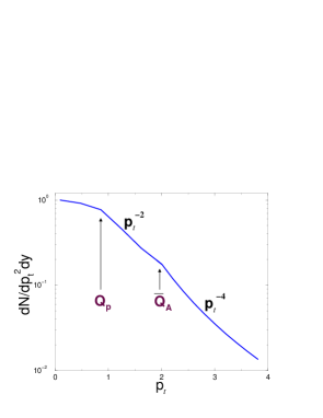
FIG. 2.: Schematic distribution of the $p_{t}$ distribution of produced gluons in a given class of events, as determined by the saturation momentum of the proton $Q_{p}$ (or, equivalently, by $dN/dy$). $\overline{Q}_{A}$ denotes the average saturation momentum of the nucleus.

The transverse momentum distribution within one event class therefore has the shape depicted in Fig. 2. At very small transverse momentum $p_{t}\mathrel{\lower 3.87495pt\hbox{$\stackrel{{\scriptstyle\displaystyle<}}{{\sim}}$}}Q_{p}$, the distribution appears rather flat [13]. Here, both the field of the proton as well as that of the nucleus are in the nonlinear “saturation” regime. As discussed above, the width of this region is proportional to the square root of $dN/dy$. For the highest multiplicity classes, when $dN/dy$ is about $200^{1/3}\simeq 6$ times larger than on average, this region of transverse momenta could extend all the way up to $\overline{Q}_{A}$. In turn, for low multiplicity events it will shrink.

Above $Q_{p}$, up to about the average nuclear saturation momentum $\overline{Q}_{A}$ the gluon distribution drops approximately like $1/p_{t}^{2}$. This is the regime where the proton field is weak but that of the nucleus still is “saturated”. It can extend down to small transverse momentum for the lowest multiplicity class, or could be “squeezed” completely at very large $dN/dy$.

For a closer look at the $p_{t}$ distributions in different multiplicity classes it is useful to divide the distributions from each class by that corresponding to the highest multiplicity bin, forming the ratio

$$R(p_{t};Q_{p}^{2})=\frac{dN}{dp_{t}^{2}\,dy}(Q_{p}^{2})\left(\frac{dN}{dp_{t}^{2}\,dy}(Q^{2}_{p,{\rm max}})\right)^{-1}~{}.$$ (29)

This should be flat at small transverse momenta, $p_{t}\mathrel{\lower 3.87495pt\hbox{$\stackrel{{\scriptstyle\displaystyle<}}{{\sim}}$}}Q_{p}$. Above $Q_{p}$ it drops since ${dN}/{dp_{t}^{2}\,dy}(Q_{p}^{2})$ decreases while ${dN}/{dp_{t}^{2}\,dy}(Q^{2}_{p,{\rm max}})$ is approximately constant. Above $Q_{A}$ finally, the ratio flattens and becomes constant since from eq. (20) the distributions in the various multiplicity bins become proportional.

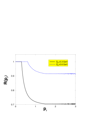
FIG. 3.: $p_{t}$ distributions in various multiplicity bins relative to that in the highest-multiplicity bin.

Fig. 3 shows the behavior of $R(p_{t})$. For this figure, the $p_{t}$ distributions were taken to be

$$\frac{dN}{dp_{t}^{2}\,dy} = \frac{1}{p_{t}^{2}+\Lambda^{2}}~{},\quad\quad\quad(p_{t}<Q_{p})$$ (30)

$$= \frac{Q_{p}^{2}}{p_{t}^{2}(Q_{p}^{2}+\Lambda^{2})}~{},\quad(Q_{p}<p_{t}<Q_{A})$$ (31)

$$= \frac{Q_{p}^{2}Q_{A}^{2}}{p_{t}^{4}(Q_{p}^{2}+\Lambda^{2})}~{},\quad(p_{t}>Q_{A})~{},$$ (32)

with the cutoff $\Lambda=0.2$ GeV, the nuclear saturation scale $Q_{A}=1.5$ GeV and $Q_{p,{\rm max}}=Q_{A}$. These numbers may be reasonable for the central rapidity region of $p+Au$ collisions at RHIC energy. For LHC they are expected to be bigger by about a factor $\exp(\lambda(y_{\rm LHC}-y_{\rm RHIC})/2)\simeq 1.7$, where $y_{\rm LHC}\simeq 8.8$ and $y_{\rm RHIC}\simeq 5.4$ are the beam rapidities at the two colliders, and the intercept $\lambda\simeq 0.3$ [20].

The broadening of the $p_{t}$ distributions with increasing multiplicity then leads to an increase of $\langle p_{t}\rangle$ with $dN/dy$; at least as long as $Q_{p}\ll Q_{A}$, $\langle p_{t}\rangle$ was shown to scale with the square root of $dN/dy$ [15, 16]. This may lead to changes of multiparticle correlations [21] with increasing $dN/dy$. Moreover, at midrapidity, the inelastic cross section is dominated by scattering of small-$x$ gluons and a nearly flavor symmetric sea of (anti-)quarks. Therefore, when the typical transverse momentum of produced gluons becomes larger than typical hadronic mass scales, the hadronic final state should as well be nearly flavor symmetric. It might be impossible to achieve sufficiently large $\langle p_{t}\rangle$ at either RHIC or LHC to be able to neglect, as an example, the masses of the kaons. Nevertheless, it would be very interesting to see whether multiplicity ratios for e.g. $K^{\pm}$ to $\pi^{\pm}$ (or $\eta$ to $\pi^{0}$) do increase at all with the multiplicity of the event. Experimentally, this is not seen for $p\bar{p}$ collisions up to Tevatron energies [22]. It might be related to the fact that the correlation length for thermal Wilson lines at confinement is large, on the order of the proton radius [23].

Finally, it may be interesting to consider the distribution of leading hadrons (in the proton fragmentation region) which are produced by fragmentation of large-$x$ quarks from the proton [18], similar to Deep Inelastic $eA$ scattering [24]. Far from the beam rapidity of the nucleus, its saturation momentum increases by a factor $\exp(\lambda y)$ relative to that at central rapidity, while in turn $Q_{p}$ decreases by the same factor. The quarks from the incident proton are then scattered to rather large transverse momenta of order $Q_{A}$, and the shape of the forward $p_{t}$ distribution should depend less on $Q_{p}$. That is, $dN/Q_{p}^{2}\,dp_{t}^{2}\,dy$ should approach a “limiting shape”, which depends rather weakly on the event multiplicity $dN/dy$ (or $Q_{p}$).

In summary, experimental analysis of the multiplicity distributions in high-energy $pA$ collisions, and of correlated changes of the $p_{t}$ distributions could provide some fundamental insight into the effective action for small-$x$ gluons, provided that a semi-classical distribution over saturation momenta exists and that it is not overwhelmed by higher-order corrections in $\alpha_{s}$.

Acknowledgements: I thank Jamal Jalilian-Marian, Mark Strikman, and Raju Venugopalan for useful discussions, the DOE for support from Grant DE-AC02-98CH10886, and the organizers of the workshop “Coherent Effects at RHIC and LHC: Initial Conditions and Hard Probes”, ECT*, Trento (Italy), October 14-25, 2002, http://pluto.mpi-hd.mpg.de/trento, where part of this work was presented.

REFERENCES

- [1] L. V. Gribov, E. M. Levin and M. G. Ryskin, Phys. Rept. 100, 1 (1983); A. H. Mueller and J. Qiu, Nucl. Phys. B 268, 427 (1986).
- [2] L. McLerran and R. Venugopalan, Phys. Rev. D 49, 2233 (1994), ibid. 49, 3352 (1994); ibid. 59, 094002 (1999).
- [3] Y. V. Kovchegov, Phys. Rev. D 54, 5463 (1996); ibid. 55, 5445 (1997); ibid. 61, 074018 (2000).
- [4] I. Balitsky, Nucl. Phys. B 463, 99 (1996).
- [5] J. Jalilian-Marian, A. Kovner, L. McLerran and H. Weigert, Phys. Rev. D 55, 5414 (1997); J. Jalilian-Marian, A. Kovner, A. Leonidov and H. Weigert, Nucl. Phys. B 504, 415 (1997); Phys. Rev. D 59, 014014 (1999); ibid. 59, 034007 (1999) [Erratum-ibid. 59, 099903 (1999)]; J. Jalilian-Marian, A. Kovner and H. Weigert, ibid. 59, 014015 (1999); A. Kovner and J. G. Milhano, ibid. 61, 014012 (2000); A. Kovner, J. G. Milhano and H. Weigert, ibid. 62, 114005 (2000).
- [6] E. Iancu, A. Leonidov and L. D. McLerran, Phys. Lett. B 510, 133 (2001); Nucl. Phys. A 692, 583 (2001); E. Ferreiro, E. Iancu, A. Leonidov and L. McLerran, ibid. 703, 489 (2002); E. Iancu, arXiv:hep-ph/0210236.
- [7] A. H. Mueller, Nucl. Phys. B 558, 285 (1999).
- [8] A. Kovner and U. A. Wiedemann, Phys. Rev. D 66, 051502 (2002); ibid. 66, 034031 (2002).
- [9] H. J. Pirner, Phys. Lett. B 521, 279 (2001); H. J. Pirner and F. Yuan, Phys. Rev. D 66, 034020 (2002).
- [10] C. S. Lam and G. Mahlon, Phys. Rev. D 64, 016004 (2001).
- [11] B. Svetitsky and L. G. Yaffe, Nucl. Phys. B 210, 423 (1982); R. D. Pisarski, Phys. Rev. D 62, 111501 (2000); A. Dumitru and R. D. Pisarski, Phys. Lett. B 525, 95 (2002); arXiv:hep-ph/0204223; T. R. Miller and M. C. Ogilvie, Phys. Lett. B 488, 313 (2000); P. N. Meisinger, T. R. Miller and M. C. Ogilvie, Phys. Rev. D 65, 034009 (2002).
- [12] J. Hofmann, H. Stöcker, U. W. Heinz, W. Scheid and W. Greiner, Phys. Rev. Lett. 36, 88 (1976).
- [13] A. Krasnitz, Y. Nara and R. Venugopalan, arXiv:hep-ph/0209269; Phys. Rev. Lett. 87, 192302 (2001).
- [14] X. N. Wang and M. Gyulassy, Phys. Rev. D 45, 844 (1992).
- [15] A. Dumitru and L. McLerran, Nucl. Phys. A 700, 492 (2002).
- [16] A. Dumitru and J. Jalilian-Marian, Phys. Lett. B 547, 15 (2002).
- [17] Yu. Kovchegov and A.H. Mueller, Nucl. Phys. B 529, 451 (1998); B.Z. Kopeliovich, A.V. Tarasov and A. Schäfer, Phys. Rev. C 59, 1609 (1999).
- [18] A. Dumitru and J. Jalilian-Marian, Phys. Rev. Lett. 89, 022301 (2002).
- [19] L. Frankfurt and M. Strikman, Phys. Rev. Lett. 66, 2289 (1991); H. Heiselberg, G. Baym, B. Blaettel, L. L. Frankfurt and M. Strikman, ibid. 67, 2946 (1991).
- [20] K. Golec-Biernat and M. Wüsthoff, Phys. Rev. D 59, 014017 (1999); J. Bartels, K. Golec-Biernat and H. Kowalski, ibid. 66, 014001 (2002); A. H. Mueller and D. N. Triantafyllopoulos, Nucl. Phys. B 640, 331 (2002); D. N. Triantafyllopoulos, arXiv:hep-ph/0209121; A. Freund, K. Rummukainen, H. Weigert and A. Schaefer, arXiv:hep-ph/0210139.
- [21] Y. V. Kovchegov and K. L. Tuchin, Nucl. Phys. A 708, 413 (2002); arXiv:nucl-th/0207037.
- [22] T. Alexopoulos et al., Phys. Rev. D 48, 984 (1993).
- [23] O. Scavenius, A. Dumitru and J. T. Lenaghan, Phys. Rev. C 66, 034903 (2002).
- [24] L. Frankfurt, V. Guzey, M. McDermott and M. Strikman, Phys. Rev. Lett. 87, 192301 (2001).