UCL/HEP 2002-04
October 2002

JetWeb: A WWW Interface and Database for Monte Carlo Tuning and Validation

J. M. Butterworth
S. Butterworth

Department of Physics & Astronomy
University College London
Gower St. London WC1E 6BT
England

A World Wide Web interface to a Monte Carlo validation and tuning facility is described. The aim of the package is to allow rapid and reproducible comparisons to be made between detailed measurements at high-energy physics colliders and general physics simulation packages. The package includes a relational database, a Java servlet query and display facility, and clean interfaces to simulation packages and their parameters.

PACS:
Keywords: Monte Carlo simulation; QCD Final States; Jets; Database; Java; MySQL; WWW

1 Introduction

We present a web-based facility for the comparison of measurements of hadronic final states and the expectations of physics calculations and simulations. The physics motivation is discussed. Then follows an outline of the design and technology used in the JetWeb server. Section 4 contains a user guide to the server, as presented on the web, while Sections  5 and  6 cover the implementation of the server with a view to further development and future plans.

2 The physics problem

Particle physics experiments at high-energy accelerators have provided a wealth of data on the final state in electron-positron, lepton-proton and proton-antiproton interactions. These data have seen the triumph of the standard model in precision electroweak measurements and the verification of the QCD sector of the standard model to a reasonable degree of precision.

Despite these successes, the final state in hadron-hadron collisions is in general poorly understood. The hadronisation stage of a collision is not calculable in perturbative QCD, and calculations of (for example) multijet production are impractical at higher orders in QCD. Other problems include the description of non-perturbative remnant-remnant interactions, and the determination of the intrinsic transverse momentum of partons in the incoming hadron. All these areas are calculated and/or modelled to some degree in general purpose Monte-Carlo simulation programs such as Pythia [1] and Herwig [2]. These packages provide an invaluable tool in several distinct ways.

• They provide physically motivated input to detector simulations, thus facilitating the evaluation of acceptances and resolutions for detectors.

• They allow the estimation of the effects of hadronisation and other uncalculated effects on cross sections so that physically observable hadronic cross sections may be compared to partonic variables calculated to high orders in QCD.

• They allow predictions to be made for collisions at future colliders, which are vital input to the motivation and design of facilities.

For all these reasons, consistent tuning of the free parameters of these generators, and confirmation of the physics assumptions they contain, is of critical importance for the accuracy and interpretation of measurements at current and future high-energy colliders. However, determining whether such models are consistent with the wide range of available data is a non-trivial matter since the measurements are made with a variety of colliding beams, in many different regions of phase space, and for many complex observables. Detailed and successful fits have been performed using LEP data but these give no information on physics specific to incoming hadrons. In addition, there is an urgent need for the preservation of expertise and access to this data.

The JetWeb server is designed to provide the ability to compare quickly and efficiently existing or future calculations and models with all relevant collider data. This is an ambitious and long term (indeed indefinite) task. Currently a subset of HERA, LEP and Tevatron jet data are included and only the Herwig and Pythia generators are used. However, the server is designed to be scalable, with clean interfaces between the various technologies used for ease of development and maintenance and the inclusion of new data and simulations.

3 The JetWeb server

The components of the JetWeb server and their functions and interactions are illustrated in Figure 1.

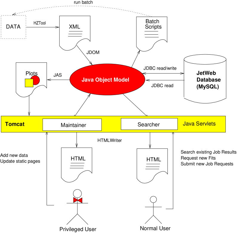
Figure 1: Components of the JetWeb server.

At the centre of JetWeb is a java object model (Figures  2 and  3) containing the properties and interactions of Models, Papers, Plots and Fits. The data underlying this model are stored in the JetWeb database - a MySQL database (Figure 4). The approximate correspondences between tables and object model classes are given in Table 1.

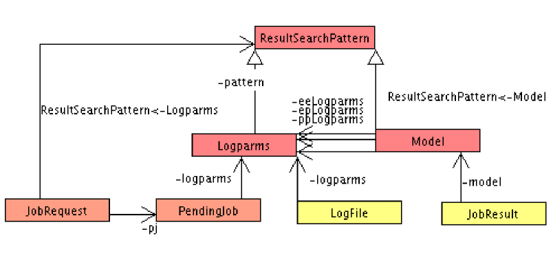
Figure 2: JetWeb Object Model: ResultSearchPattern. ResultSearchPattern is a container for a set of parameters specifying a database search. Model and Logparms are both specialised types of ResultSearchPattern. A Model specifies a complete set of parameters including a unique generator but not a collider, while a Logparms defines a unique collider along with the subset of parameters it requires. JobRequest, PendingJob and Logfile all describe a single batch job with parameters specifed by a Logparms. JobRequest is constructed from a ResultSearchPattern; that is, the ResultSearchPattern parameters specify the job to be run. PendingJob is built when a JobRequest is submitted and exists to provide status information about unfinished batch jobs. Logfile is built from the output log file of a batch job. A JobResult is constructed from a Model and a set of data to which it is compared.

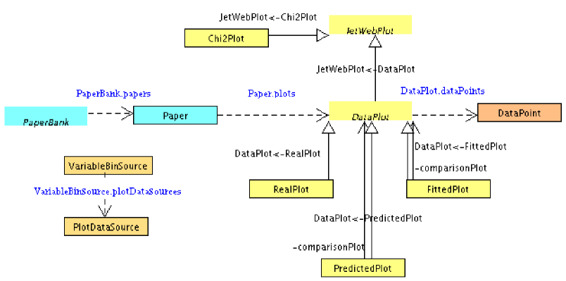
Figure 3: JetWeb Object Model: Papers and Plots. Data is held in the object model in this series of paper and plot objects. At the top level, PaperBank is a container for all the papers. Each Paper contains a collection of plots. JetWebPlot is the fundamental plot class and incorporates JAS functionality to output gifs and also includes the plotML read/write methods. There are three types of DataPlot; RealPlot (real measured data from experiments), PredictedPlot (MC data) and FittedPlot (MC data that has been compared to real data). Chi2Plot is not a type of DataPlot. It plots $\chi^{2}$ scatter for a selection of fits. Each DataPlot contains a set of DataPoints. VariableBinSource is a container for a set of plot data sources to handle variable bin histograms. PlotDataSource is the JetWeb 1D Histogram object, and is the jetweb implementation of the JAS interface Rebinnable1DHistogramData. A PlotDataSource can be constructed from a set of DataPoints allowing a histogram to be written from a DataPlot. NB, classes represented by unbounded boxes are Abstract.

Class	Table
Logparms	logparms
	herwig_parameters
	pythia_parameters
Model	model
	herwig_model
	pythia_model
JobResult	fit
Paper	paper
RealPlot	crossection
DataPoint	data_point
PredictedPlot	crossection
DataPoint	predicted_point
FittedPlot	fitted_prediction
DataPoint	fitted_point
LogFile	logfile
PlotSelection	crosssection_set

Table 1: Approximate correspondence between classes in the object model and tables in the database.

A “Model” completely specifies a unique generator, version and set of parameters. A “Logparms” consists of a subset of these parameters relevant to a specific set of colliding beams (for example, proton-proton logparms do not define a photon parton distribution, and photon-photon logparms likewise do not specify a proton parton distribution). Consquently one model can currently have up to three logparms associated with it ($ee$, $ep$ and $pp$). A “Logfile” for an individual simulation run is associated with a single logparms. A “Paper” encapsulates the measured data from a single publication and is associated with measured cross sections. A “Fit” contains the results of a comparison between real data and the predictions of a specific model. For more detail on the constituents of the object model, see Figures 2 and  3.

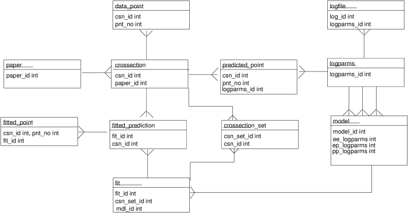
Figure 4: JetWeb Database. The diagram shows the tables of the JetWeb database, their primary keys, the relationships between the tables and the fields on the tables pertaining to those relationships. A paper (identified by paper_id) may have one or more crosssections, while each crosssection record (identified by a csn_id) has a single paper_id associated with it. A crosssection (equivalent to Plot in the java object model) may have a set of data_points or predicted_points or a fitted_prediction. A fit compares a model to a set of crosssections, as specified by its crosssection_set. Each model may have up to three associated logparms records; one each for electron-electron, electron-proton and proton-proton.

Data is added to the database as follows:

• MC results from HZTOOL [3] are processed by a FORTRAN routine which reads in HBOOK [4] histogram files and writes out histograms in the form of XML files in the Java Analysis Studio [9] (JAS) plotML DTD format [5].

• The JetWeb XMLReader facility is a Java class, used to convert plotML data into the Java object model. It processes the XML data using the JDOM API [6], wrapping a SAX parser.

• Data held within the Java object model is written to the JetWeb database via JDBC [7]. The interface between object model and database is provided by the database manager classes within the ucl.hep.jetweb.db package.

These stages are initiated by commands from the Maintainer (privileged access user interface, see below). The user accesses JetWeb via the web user interface (UI), which consists of Java servlets run on a Tomcat [8] server, delivering HTML pages written using the JetWeb HTMLWriter facility (ucl.hep.jetweb.html package). The servlets access the JetWeb database via the JDBC calls encapsulated within the java object model.

There are two levels of access to JetWeb:

• Normal access allows the user to query the JetWeb database for existing Job Results. The user can fit these results to the data from a range of papers stored on the database.

  Fit data is loaded from the database into the object model. If this fit has been requested before, the static webpages will already exist. A comparison is made between the timestamp in the database and the date of these pages. If the pages are more up-to-date, they are served to the user (This avoids the extremely time consuming regeneration of histogram graphics files). If the pages predate any relevant data in the database they are regenerated. In this case an HTML summary of the fit is written, and ucl.hep.jetweb.plots.DataPlot and its subclasses access JAS to write gif plot files. Plot files are incorporated into HTML generated by servlets using the HTMLWriter utility. The graphics generation is done in a separate thread to improve response time for the user.

  If there are no results stored for the user’s specified set of parameters, a new job request with the required parameters can be generated. The job requests are moderated and submitted by an administrator on the server side.

• Privileged access is available to allow maintenance of the JetWeb Server. It allows the update of the static webpages associated with the application. It controls the upload of new data to the JetWeb database. It also manages the running of new batch jobs, facilitating submission of new jobs and monitoring of incomplete runs.

4 User guide

This section outlines the expected use of the web pages (http://jetweb.hep.ucl.ac.uk) for a normal (unprivileged) user.

The top-level welcome page (Figure 5) provides the user with several options. Down the left hand side are various short cuts to static web pages. These include

• A short-cut to the current best fit for each simulation package used.

• Lists of all fits currently in the database.

• An extensive bibliography with references to the data used in JetWeb, presentations using results from JetWeb, and other related work.

• Documentation of the simulations currently available in HZTOOL.

• Links to the experiments whose data are used in JetWeb.

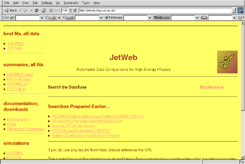
Figure 5: JetWeb Application Welcome page.

In the central section of the page are links allowing the user to

• Query the database directly

• Access previously prepared searches

4.1 Querying the database for existing results

4.1.1 Prepared searches

A selection of standard queries relating to specific parameters or physics studies are listed on the JetWeb welcome page. Following the links from here gives access to all the fits as well as a summary of conclusions to be drawn from them.

4.1.2 Interactive searches

On the welcome page, clicking ‘Search the Database’ causes a parameter input form to be displayed, as shown in Figure  6.

• Common parameters; various parameters common to all generators can be entered on first part of form

• Generator specific parameters: The search may be restricted to specialised parameters for a particular generator. Currenly HERWIG and PYTHIA are implemented.

  • HERWIG parameters. Check Generator - HERWIG. Click ‘Change HERWIG parameters’. This will display additional fields for the HERWIG parameters to be entered.

  • PYTHIA parameters. Check Generator - PYTHIA. Click ‘Change PYTHIA parameters’. Boxes will be displayed to enter the number and value of each MSTP and PARP parameter to be specified. Enter the values and press ‘Add’. MSTP and PARP parameters which have been set will be displayed on the form. To remove a value, enter its number in the relevant field, but leave the corresponding box blank, then press ‘Add’. Specify all the parameters required in this way before continuing with the search.

• The sort order of results can be specified by choosing a value from the ‘sort results…’ list at the top of the form.

• Results can be filtered by selecting a value for the ‘only show results..’ list at the top of the form. Some models in the database will have been compared to a subset of the available data only. This option allows the user to exclude any models that have not been compared to the chosen data.

• Submit a search by clicking ‘Get Results’ at the top of the form.

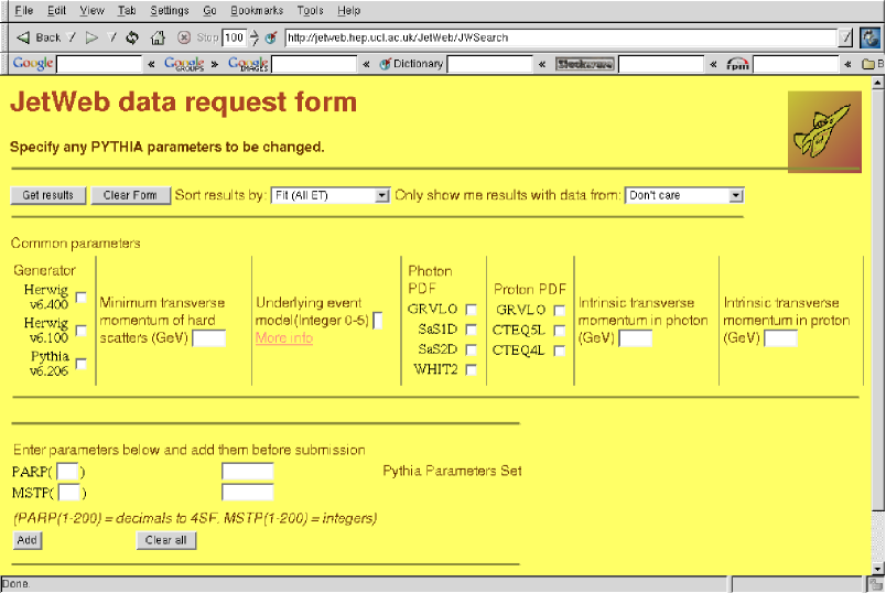
Figure 6: JetWeb Search Page.

4.1.3 Query output

If a search is successful, brief summaries of the available results will be listed. Each Job Result will also have a link (‘Plots etc’) for access to a detailed description of the Fit and the actual histograms showing the comparison (Figure 7).

If there are no data corresponding to the input search parameters, the JetWeb Request form will be displayed with the required parameters filled in. From here, a request can be made for a new job to be run.

4.2 Request new jobs

Job requests can be made in two contexts

• Search fails to find results - this brings up the JobRequest form with the failed search parameters filled in.

• A request for additional data can be made from the Fit Details page, Figure 7, for each job. First, the collider must be selected. More data for a particular collider (with unchanged job parameters) can be requested using the ‘Request highwer statistics’ option, while ‘Request similar data’ allows a new job to be specified with altered parameters. The latter option accesses the job request form, allowing the user to vary a subset of parameters while guaranteeing that all others will remain identical to those of the originally selected fit.

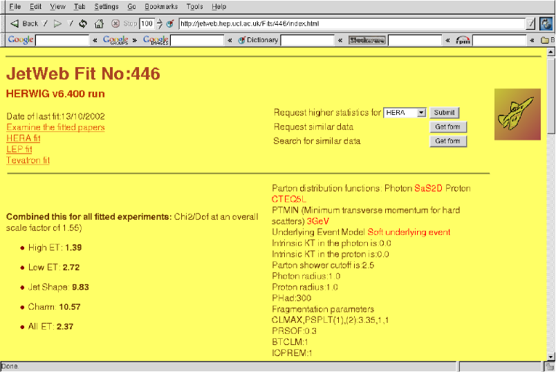
Figure 7: Fit Details Page.

5 Developer guide

This section is intended to outline ways in which the application could be altered or enhanced to expand its scope. It should be used as a guide for developers in conjunction with JavaDoc for the JetWeb java application, and other documentation on the JetWeb website (jetweb.hep.ucl.ac.uk).

5.1 To switch database

MySQL is a simple relational SQL database with a JDBC driver available. The database is accessed from the java object model using the ucl.hep.jetweb.db package. Minimal changes would be required to convert to another SQL database (probably just changing the relevant JDBC driver). For conversion to a different type of database, new database manager classes would be required, implementing the same interface as the existing DBManager, DBFitManager and DBPlotManager.

5.2 To switch user interface

The interface of the ucl.hep.jetweb.servlet package would have to be implemented by any alternative UI. This application was originally run using a Java Swing UI. It should be very straightforward to implement a simple command-line interface. A new UI would replace the ucl.hep.jetweb.servlet package; accessing the same methods on ucl.hep.jetweb.ResultManager.

5.3 To add new measurements

There is a main method on Paper which adds new RealPlots to the database. To produce new PredictedPlots, the appropriate HZTool routines must be provided and called, and the Fortran modified to output XML data files for the new histograms.

5.4 To add a new simulation package

The major work here would be to interface the new package to HZTool (or an equivalent package capable of producing suitable output files - see below). In addition, tables would have to be added to the database specifying any extra parameters needed to define a model with the new simulation package.

5.5 To add information or new formatting to the web pages

The ucl.hep.jetweb.html package and specifically the HTMLWriter class is responsible for constructing the JetWeb web pages. Thus, changing the layout or content of these pages necessitates modification of this class’s methods.

5.6 To add servlet queries

The user requests fits by filling in an HTML form. A ucl.hep.jetweb.ResultSearchPattern and a ucl.hep.jetweb.PlotSelection are built from the HTML form. A database query is constructed from these objects. To add new parameters to user queries, the relevant fields must be added to ResultSearchPattern and PlotSelection, and the database query methods updated to incorporate these new fields.

5.7 To add HTML queries

The prepared searches available from the welcome page are simple HTML forms that are submitted to the server. These forms can be used as templates for users to prepare their own standard (or often repeated) searches.

5.8 To input data

5.8.1 XML

Data is loaded into the JetWeb application in the form of XML files generated by the HZTool FORTRAN routine. The format of these files is derived from the JAS DTD - plotML. Although the XML files produced are valid plotML files, in fact only a subset of the elements in plotML are used. Thus, the JetWeb XML format can also be represented by a reduced size plotML (Figures 8 and  9). An example XML file using this reduced plotML DTD is included in the appendix. The ucl.hep.jetweb.plots.JetWebXMLReader reads in XML documents (reduced plotML format) using the JDOM utility [6]. JetWebXMLReader will ignore any additional elements present in the files. The XMLReader utility could also be adapted to read

• a wider range of plotML documents;

• a different XML format.

However, it would be simpler to retain the original plotML Reader and use an XSL stylesheet to convert between XML formats, if this should be required.

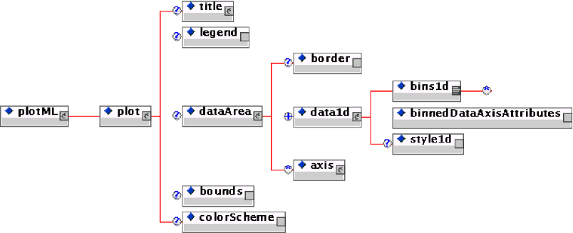
Figure 8: PlotML DTD - JetWeb reduced version. This is a graphical representation of the tree-like format of plotML. plotML is the root element of the document. Each reduced plotML document contains a single plot element, made up of title, legend, bounds, colorScheme and the central dataArea. This dataArea element has a border, an axis element and one or many data1d elements (see Figure 9). This represents a major simplification of the original plotML which, for example, also includes 2-dimensional histograms and scatter plots.

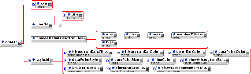
Figure 9: JetWeb 1D Histogram Data Element . Agraphical representation of the data1d element of the jetweb reduced version of plotML.The axes are specified within the binnedDataAxisAttributes, while styleId specifies the appearance of the plot. The data points themselves are held within the bins1d element in a single (potentially very long) string, with each point separated by a carriage return. For more detail, see appendix and the JAS documentation;  [5].

One consequence of adopting the plotML input format for the java object model is that any program capable of producing plotML histograms can be used to provide simulation data for JetWeb. Currently a Fortran routine (h2XML) is provided (and is available from the web pages) to convert HBOOK histograms to the reduced plotML format described above. To allow JetWeb to read data from other formats, similar conversion facilities would be required.

5.9 To output data

5.9.1 HTML

The ucl.hep.jetweb.html package is responsible for producing the web front end for JetWeb. Some of the classes (including Paper, DataPlot and JobResult) have toHTML methods. These should really be migrated to the HTML package in future releases.

5.9.2 XML

The JDOM functionality could be used in an XMLWriter class which would reconstruct the XML documents from the object model. The documents could be constructed in plotML, or another DTD.

5.9.3 XML, HTML, any text format

XSL stylesheets can be used to convert XML documents from one format to another. If several formats were required, only a single XMLWriter utility, used in conjunction with stylesheets, could produce multiple output formats including XML, HTML - allowing direct visualisation of data on a webpage - and plain text.

5.9.4 Plots

ucl.hep.jetweb.plots.DataPlot and its subclasses can be output as gif files using the JAS utility. This utility is still under development and supports an increasing variety of output formats, including encapsulated postscript. If an unsupported format of plot file were required, it would probably be simplest to extract the data in XML format to be submitted to the plotting facility.

5.10 Batch job submission

Job submission from the server side is made in several ways. There are options for submission to UK particle physics grid [10] as well as direct submission to local batch systems. This is transparent to the general user. To submit to new facilties, template scripts must be provided and the extra protocols added to the ucl.hep.jetweb.script package.

6 Future plans

There are several obvious and important developments of the JetWeb facility which should take place. Some of these are described below.

Server side submission of jobs to the Grid has already been implemented. It is also likely that the database itself will become directly accessible as a grid data resource.

The Fortran library HZTOOL should eventually be augmented or replaced by a similar package following an object-oriented design. This is motivated by the advantages of OO design principals, the declining knowledge base in Fortran and the likely future requirement to validate C++ versions of the general purpose generators, PYTHIA7 & HERWIG++, which are currently under development.

In addition to the new versions of those generators, several next-to-leading order QCD generators are under development and these could be tested with this facility.

Finally, there are major data sets and classes of data which should be added to a truly ‘global’ validation facility, for example LEP and SLD hadronic data from the $Z$, HERA deep inelastic scattering data and data from proton machines other than the Tevatron.

Appendix

6.1 HZTool XML output file - example

<?xml version="1.0" encoding="ISO-8859-1" ?>
<!DOCTYPE plotML SYSTEM "plotML.dtd">
<plotML>
  <plot>
    <title>
      <border type="None"/>
      <label text="Jet ET &gt; 4 GeV">
        <font style="BOLD" points="14" face="SansSerif"/>
      </label>
    </title>
    <legend visible="never">
    </legend>
    <dataArea>
      <border type="None"/>
      <!--
ΨEach of the following data1d elements contains a single point.
ΨThis handles variable bin widths.
Ψ(For a constant bin width histogram,
Ψ only one data1d element would be required,
Ψ with all data points in a single string,
Ψ separated by carriage returns)
       -->
      <data1d axis="y0">
        <bins1d title=" ">
          0.49,0.14,0.14
        </bins1d>
        <binnedDataAxisAttributes max="-1.4" numberOfBins="1"
          min="-1.15" type="double" axis="x"/>
        <style1d dataPointSize="6" showErrorBars="true"
          histogramBarsFilled="true" showLinesBetweenPoints="false"
          errorBarColor="Black" dataPointStyle="dot" showHistogramBars="false"
          lineColor="Black" dataPointColor="Black" showDataPoints="true"
          histogramBarColor="Blue"/>
      </data1d>
      <data1d axis="y0">
        <bins1d title=" ">
          0.88,0.22,0.22
        </bins1d>
        <binnedDataAxisAttributes axis="x" numberOfBins="1"
          min="-0.8999999999999999" type="double" max="-1.15"/>
        <style1d dataPointSize="6" showErrorBars="true"
          histogramBarsFilled="true" showLinesBetweenPoints="false"
          dataPointStyle="dot"
          errorBarColor="Black" showHistogramBars="false" lineColor="Black"
          dataPointColor="Black" showDataPoints="true"
Ψ  histogramBarColor="Red"/>
      </data1d>
      <data1d axis="y0">
        <bins1d title=" ">
          0.92,0.24,0.24
        </bins1d>
        <binnedDataAxisAttributes axis="x" numberOfBins="1"
          min="-0.7" type="double" max="-0.9000000000000001"/>
        <style1d dataPointSize="6" showErrorBars="true"
          histogramBarsFilled="true" showLinesBetweenPoints="false"
ΨdataPointStyle="dot"
          errorBarColor="Black" showHistogramBars="false" lineColor="Black"
          dataPointColor="Black" showDataPoints="true"
Ψ  histogramBarColor="Fuchsia"/>
      </data1d>
      <data1d axis="y0">
        <bins1d title=" ">
          0.83,0.14,0.14
        </bins1d>
        <binnedDataAxisAttributes axis="x" numberOfBins="1"
          min="-0.5" type="double" max="-0.7"/>
        <style1d dataPointSize="6" showErrorBars="true"
          histogramBarsFilled="true" showLinesBetweenPoints="false"
Ψ  dataPointStyle="dot"
          errorBarColor="Black" showHistogramBars="false" lineColor="Black"
          dataPointColor="Black" showDataPoints="true"
          histogramBarColor="Yellow"/>
      </data1d>
      <data1d axis="y0">
        <bins1d title=" ">
          0.85,0.17,0.17
        </bins1d>
        <binnedDataAxisAttributes axis="x" numberOfBins="1"
          min="-0.30000000000000004" type="double" max="-0.5"/>
        <style1d dataPointSize="6" showErrorBars="true"
          histogramBarsFilled="true" showLinesBetweenPoints="false"
Ψ  dataPointStyle="dot"
          errorBarColor="Black" showHistogramBars="false" lineColor="Black"
          dataPointColor="Black" showDataPoints="true"
          histogramBarColor="Lime"/>
      </data1d>
      <data1d axis="y0">
        <bins1d title=" ">
          0.78,0.14,0.14
        </bins1d>
        <binnedDataAxisAttributes axis="x" numberOfBins="1"
          min="-0.10000000000000003" type="double" max="-0.3"/>
        <style1d dataPointSize="6" showErrorBars="true"
          histogramBarsFilled="true" showLinesBetweenPoints="false"
Ψ  dataPointStyle="dot"
          errorBarColor="Black" showHistogramBars="false" lineColor="Black"
          dataPointColor="Black" showDataPoints="true"
          histogramBarColor="Orange"/>
      </data1d>
      <data1d axis="y0">
        <bins1d title=" ">
          0.54,0.12,0.12
        </bins1d>
        <binnedDataAxisAttributes axis="x" numberOfBins="1"
          min="0.04000000000000001" type="double" max="-0.1"/>
        <style1d dataPointSize="6" showErrorBars="true"
          histogramBarsFilled="true" showLinesBetweenPoints="false"
Ψ  dataPointStyle="dot"
          errorBarColor="Black" showHistogramBars="false" lineColor="Black"
          dataPointColor="Black" showDataPoints="true"
          histogramBarColor="Aqua"/>
      </data1d>
      <axis logarithmic="false" showOverflows="false"
        numberOfBins="50" allowSuppressedZero="true" type="double"
        location="x0">
        <label text="xgamma">
          <font style="PLAIN" face="Dialog" points="12"/>
        </label>
        <font style="PLAIN" face="Dialog" points="12"/>
      </axis>
      <axis logarithmic="false" showOverflows="false" min="0.0"
        allowSuppressedZero="true" type="double" max="1.0120000000000002"
Ψlocation="y0">
        <label text="d(sigma)/d(xgamma) (nb)">
          <font style="PLAIN" face="Dialog" points="12"/>
        </label>
        <font style="PLAIN" face="Dialog" points="12"/>
      </axis>
    </dataArea>
    <bounds width="400" height="400"/>
    <colorScheme foregroundColor="default"
      backgroundColor="(255,215,0)"/>
  </plot>
</plotML>

References

- [1] T. Sjöstrand et al, Computer Phys. Commun. 135 (2001); hep-ph/0010017.
- [2] G. Corcella et al, JHEP 0101 (2001) 010 hep-ph/0011363; hep-ph/0201201.
- [3] J. Bromley et al, Hamburg 1995/96, Future physics at HERA, vol. 1, 611-612.
- [4] R. Brun, D. Lienart. CERN-Y250, Oct 1987.
- [5] http://www-sldnt.slac.stanford.edu/jas/Documentation/ howto/xml/default.shtml
- [6] http://www.jdom.org/
- [7] M. Matthews, http://mmmysql.sourceforge.net/old-index.html http://www.mysql.com/downloads/api-jdbc.html
- [8] Tomcat http://jakarta.apache.org/tomcat
- [9] A.S. Johnson, CHEP 2000, Computing in high-energy and nuclear physics, 741-745. http://jas.freehep.org/
- [10] http://www.gridpp.ac.uk/