New constraints on the running-mass inflation model
Abstract
We evaluate new observational constraints on the two-parameter scale-dependent spectral index predicted by the running-mass inflation model by combining the latest Cosmic Microwave Background (CMB) anisotropy measurements with the recent 2dFGRS data on the matter power spectrum, with Lyman forest data and finally with theoretical constraints on the reionization redshift. We find that present data still allow significant scale-dependence of , which occurs in a physically reasonable regime of parameter space.
I Introduction.
The recent observation of the cosmic microwave background (CMB) angular anisotropies toco ; b97 ; Netterfield ; halverson ; lee ; cbi ; vsa have revealed an outstanding agreement between the data and the inflationary predictions of a flat universe and of a primordial scale invariant spectrum of adiabatic density perturbations (see e.g. debe2001 ; pryke ; stompor ; wang ; cbit ; vsat ; saralewis ; mesilk ; caro ).
Furthermore, CMB measurements are in perfect agreement with other types of data and a global consistent picture is slowly emerging. For example, the CMB constraint on the amount of matter density in baryons, , is now consistent with the independent constraints from standard big bang nucleosynthesis (BBN) (see e.g. hansen ). Also, the detection of power around the expected third peak, on arc-minutes scales, provides a new and independent evidence for the presence of non-baryonic dark matter (see e.g. mesilk ). At the same time, early data releases from the 2dFGRS and SDSS galaxy redshift surveys 2dfgrs ; sdss are living up to expectations and combined analysis of all these datasets are placing strong constraints on most of the cosmological parameters efstathiou ; lahav ; mesilk . A combined analysis of both CMB and galaxy clustering is indeed necessary in order to break some of the degeneracies between the cosmological parameters that are affecting the single datasets. Recent combined analysis, for example, have provided important constraints on the amplitude of the matter fluctuations lahav ; mesilk , on the gravity waves background efstathiou , on the dark energy equation of state bean ; percival2 ; mortsell and on the neutrino mass hannestadnu ; elgaroy .
Thank to this new evidence, it is now accepted that the structure in the Universe is caused by an almost scale-independent primordial density perturbation, existing before cosmological scales start to enter the horizon. Nearly exponential inflation can easily explain the origin of this perturbation, because it converts the quantum fluctuation of every light scalar field into a scale-independent classical perturbation. At the present time, there is no equally successful alternative explanation for the origin of this perturbation. In particular, there is no reason to expect the quantum-to-classical conversion to take place in extra space dimensions, though of course a string-theoretic description of such dimensions may play a vital indirect role by determining the form of the effective four-dimensional field theory.
In this paper, we combine the latest CMB and galaxy clustering data in order to place constraints on the inflationary model responsible for the primordial density perturbation. We will in fact assume the simple paradigm of a slowly-rolling inflaton field, whose perturbations are the seed for the primordial density perturbations treview ; book 111The alternative curvaton is to make a ‘curvaton’ field responsible, different from the inflaton if indeed the latter exists.. If this hypothesis is correct, observation will be able to distinguish between the few simple and well-motivated inflation models that exist, because they give different predictions for the spectral index of the primordial density perturbation. From among such models, we focus in this paper on the running-mass model of inflation st97 ; st97bis ; clr98 ; cl98 ; c98 ; rs , which is the only one which can that can give a strongly scale-dependent (running) spectral index. Comparing with a suite of observations, we find that significant running is still allowed.
A similar attempt in constraining this kind of scale-dependence was made in cl99 and covi , where however only a limited subset of the CMB and LSS data then available was used. A model-independent approach is used instead in hannestad-run , where constraints in the plane and its first derivative were obtained. The main difference with our approach is that there it is implicitly assumed that the scale dependence is small, while this is not necessary the case for the running mass model.
Our paper is organized as follows: In section II we discuss the running mass model. In section III we present our data analysis method and results. Finally, in section IV, we discuss our conclusions.
II The Running Mass Model.
II.1 The potential
The running-mass model st97 ; st97bis ; clr98 ; cl98 ; c98 ; rs seems to be the only one which is both very well-motivated from the particle physics point of view and also presents a strong scale-dependence of the spectral index. The model is based on supersymmetry and identifies the inflaton field with a flat direction of the supersymmetric scalar potential. Global supersymmetry is broken during inflation by the large vacuum energy that drives inflation and so soft mass terms are generated for all scalar fields rsg . Taking the one-loop corrections to the tree-level potential into account, the most general expression for the potential along a flat direction, like the inflaton’s, can then be cast into the form
| (1) |
where is the soft inflaton mass and the dots indicate non-renormalizable terms which are supposed to be negligible because is exponentially small (the usually–dominant renormalizable quartic term is absent precisely because we are using a flat direction in the scalar field space). The mass dependence on the renormalization scale, in our case identified with the value of the inflaton field, is given by the renormalization group equation st97
| (2) |
and therefore is proportional to the inflaton couplings, as given below in Eq. (3).
Ignoring for the moment the running, a generic supergravity theory will generate a soft mass-squared with magnitude at least of order , which is marginally too big to support inflation. This is a problem for any model of inflation, whether or not the mass term is the one that is supposed to dominate. In all models except the running mass model, the problem is solved either by imposing a global symmetry to protect the flatness of the potential, or by supposing that the mass-squared is accidentally suppressed. The running mass model instead accepts the generic value of the mass-squared at the Planck scale (or some other high scale), and relies on the loop correction to sufficiently reduce it in the regime where inflation takes place.
For a particle with gauge and Yukawa interactions, we have that at one loop is given by st97bis ; c98
| (3) |
where the first term arises from gauge particles loops and the second from matter loops. Above are a positive group-theoretic numbers of order one, counting the degrees of freedom present in the loop, is the gauge coupling, and is the gaugino mass, while denotes a common Yukawa coupling and the common susy breaking mass-squared of the scalar particles interacting with the inflaton via Yukawa interaction. Note that the first term in Eq. (3) is always negative, while the second has no definite sign, since is defined as the mass squared splitting between scalar and fermionic superpartners and can have either sign. Also the case of a very-weakly-interacting inflaton gives and so that the constant mass potential is recovered.
Over a sufficiently small range of , or for very small inflaton couplings, it is a good approximation to take a Taylor expansion of the running mass and then we have:
| (4) |
where we have expanded around , and rescaled the last term w.r.t. for future convenience. The dimensionless constant is proportional to the mass beta function,
| (5) |
It has been shown cl98 that for small , as is required by slow roll conditions, the linear approximation is very good over the range of corresponding to horizon exit for scales between and . In order to obtain also a crude estimation of the reionization epoch via the Press-Schechter formula, which involves the power spectrum at a scale of order (enclosing the relevant mass of order ), we shall assume that the linear approximation is adequate down to this ‘reionization scale’.
For studying the inflaton potential, it is very useful to introduce a new parameter via
| (6) |
Then Eq. (7) takes the simple form cl98
| (7) |
leading to
| (8) |
In typical cases the linear approximation is valid at , and that point is then a maximum or a minimum of the potential.
The running-mass model supposes that the relevant soft masses at the Planck scale (or some other high scale) have magnitude roughly of order
| (9) |
and that the relevant couplings (gauge or Yukawa) are very roughly of order 1. In general, one of the loops will dominate over the others making only one soft mass relevant besides the inflaton mass. With these assumptions, the coupling defined by Eq. (5) is roughly
| (10) |
A bigger value of is unviable because it would not allow inflation. On the other hand, using Eq. (7) as a very crude estimate of the inflaton mass at the Planck scale, one can see that a much smaller value of is probably not viable either, since it would require the inflaton mass at that scale to be suppressed below the estimate Eq. (9).
For scalar masses, the estimate Eq. (9) is expected to be valid provided that the following statements are true: (i) there is at most gravitational-strength coupling between the inflaton sector and the sector in which SUSY is spontaneously broken (ii) this breaking comes from an term as opposed to a term (iii) during inflation (in contrast to the situation in the vacuum) the term in the potential is not accurately canceled by the other, negative contribution to the potential. The third of these requirements is reasonable provided that the potential satisfies
| (11) |
where is the SUSY-breaking scale in the vacuum.
The most economical assumption is that actually the mechanism of spontaneous SUSY breaking during inflation is basically the same as it is in the vacuum, making roughly of order . For respectively the cases of anomaly-mediated, gravity-mediated and (low-energy) gauge-mediated transmission of SUSY-breaking to the Standard Model sector, this leads to the rough estimates
| (12) | |||||
| (13) | |||||
| (14) |
The second case was assumed in the original works rsg ; st97 ; st97bis . It gives the correct normalization for the spectrum for reasonable parameters, but there is probably enough latitude to allow the first or even the third case.
We emphasize that the estimate Eq. (9) for the scalar soft masses in the inflaton sector is reasonable in all three cases, even though the soft masses in the Standard Model sector (evaluated of course in the vacuum, and of order ) satisfy that estimate only in the second, gravity-mediated case. In the first (anomaly-mediated) case, this is because no-scale supergravity does not automatically suppress soft scalar masses during inflation, as it does in the vacuum treview . In the third (gauge-mediated) case it is because one can easily suppose that the gauge-mediation mechanism simply does not operate in the inflaton sector. If the relevant soft mass is a gaugino mass, the expectation of Eq. (9) is not so automatic because gaugino masses can be very small with some types of SUSY breaking, but it is not unreasonable either.
In summary, we expect in the range (10) in a typical running mass model of inflation. As we now see, this typically leads to significant scale-dependence of the spectral index.
II.2 The spectrum and the spectral index
Now we come to the predicted spectrum and spectral index of the primordial density perturbation. We suppose that it is generated by the inflaton field perturbation, which means that it is purely adiabatic and gaussian. It is therefore specified by the curvature perturbation , with as usual the comoving wavenumber. This quantity is gaussian and hence specified by its spectrum .
To give the prediction of the running mass model for the spectrum, it is convenient to define
| (15) |
where the subscript COBE denotes the epoch of horizon exit for the COBE scale .
Instead of the spectrum we work with the conventional quantity . At the COBE scale, the prediction of the running-mass model is
| (16) |
As already mentioned, the observed value is easily obtained, for choices of and that correspond to reasonable particle physics assumptions.
In this paper we concern ourselves with the dramatic scale-dependence of the spectrum, which is given by
| (17) |
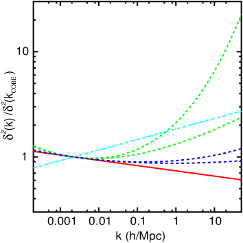
where . We plot the primordial power spectrum for the running mass model in comparison to the constant spectral index case in Figure 1.
To discuss the spectral index and its running, we need the first four derivatives of the potential,
| (18) | |||||
| (19) | |||||
| (20) | |||||
| (21) |
Introducing , the first four flatness parameters treview ; book are (setting in the denominators)
| (22) | |||||
| (23) | |||||
| (24) | |||||
| (25) |
The parameters are evaluated at the epoch of horizon exit for the scale . The first parameter is negligible because is taken to be exponentially small. The condition for slow-roll inflation is therefore just , which is satisfied in the regime provided that . This corresponds also to requiring .
Additional and generally stronger constraints on follow from the reasonable assumptions that the mass continues to run to the end of slow-roll inflation, and that the linear approximation remains roughly valid. Discounting the possibility that the end of inflation is very fine-tuned, to occur close to the maximum or minimum of the potential, we have the lower bound
| (26) |
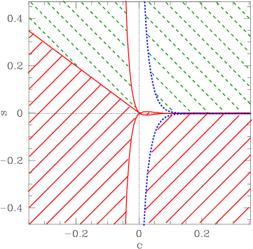
Note that for negative , this constraint is very strong, requiring a very large value of even for small and a kind of fine-tuning between and to give a reasonable value of .
For positive , we also obtain a significant upper bound by setting in Eq. (30), and remembering that slow-roll requires :
| (27) |
In the simplest case, that slow-roll inflation ends when actually becomes of order 1, this bound becomes an actual estimate, . As discussed in cl99 , this upper bound can be relaxed for positive if the running of the mass ceases before the end of slow-roll inflation. The approximate region of the versus plane excluded by these considerations is shown in Figure 2.
Since is negligible, the spectral index is
| (28) | |||||
| (29) |
This gives cl99
| (30) |
The first derivative of the spectral index is given by
| (31) |
Clearly the spectral index is not constant within cosmological unless or is very close to zero.
At the COBE scale,
| (32) | |||||
| (33) |
The straight line in the vs plane corresponds to . The scale independent case of constant is given by the origin , while constant spectral index different from is realized either on the axis for or on the axis for .
Taking cosmological scales to span a range , we see that the running mass model generates a change in the spectral index. This change should eventually be detectable unless both and are towards the bottom of their expected ranges.
We will show in the following the allowed region both in the parameter space and in the vs plane. Note in this respect that not all values of are allowed in the running mass models: from the definition above, we obtain the constraint
| (34) |
so that a decreasing spectral index is possible only if is different from 1. Also Eq. (33) is symmetric under reflection with respect to the line, so fixing the variables and determines two values of . We will investigate in the following how strongly the data are sensitive to a variation of and therefore able to disentangle this degeneracy. From all this, it follows that fitting for arbitrary value of is not exactly equivalent to performing a fit for the running mass models.
These predictions for the spectral index and its derivative are to leading order in slow-roll. To second order, the spectral index is given to a good approximation by treview
| (35) |
We neglected a term of order , and the remaining (unknown) error is expected to be of order . Both of these are negligible which means that the second-order correction should be rather accurate. We shall not include it though, because it just corresponds to a small rescaling of the quantity , whose precise value depends on unknown physics treview . Note that it is in any case easy to obtain the results at next-to-leading order, by rescaling by the factor or shift by .
III Observational constraints
III.1 Method
We compare the recent cosmological observations with a grid of theoretical models computed with the public available CMBFAST sz code. We restrict our analysis to flat, adiabatic, -CDM models and we sample the various parameters as follows: , in steps of ; , in steps of and , in steps of . The value of the Hubble constant is given by
We allow for a reionization of the intergalactic medium by varying also the compton optical depth parameter in the range in steps of . Greater values of are in disagreement with recent estimates of the redshift of reionization (see e.g. gnedin ) which points towards . As discussed later, given a cosmological model, we checked for the consistency of the assumed optical depth with its expected values derived from a simple reionization scenario.
We vary the parameters of the running mass model in the range and in a grid. To save computing time, we compute the CMB anisotropies transfer functions for each cosmological model just one time and then we integrate them different times looping over and .
For the CMB data, we use the recent results from the BOOMERanG-98, DASI, MAXIMA-1,CBI, and VSA experiments. The power spectra from these experiments were estimated in , , , and bins respectively (for the CBI, we use the data from the MOSAIC configuration), spanning the range . However, since in this work we are interested only in comparing the data with the expected primary anisotropies, we limit our analysis to the region which is likely not to be affected by secondary effects like Sunyaev-Zel’dovich (see e.g. nabila ).
The likelihood for a given theoretical model is defined by where is the Gaussian curvature of the likelihood matrix at the peak and are the experimental (theoretical) band powers. We discard the first bin of the CBI dataset (), due to the asymmetric window function and the high sample variance.
We consider , , , and Gaussian distributed calibration errors for the BOOMERanG-98, DASI, MAXIMA-1, VSA, and CBI experiments respectively and we include the beam uncertainties by the analytical marginalization method presented in sara .
In addition to the CMB data we incorporate the real-space power spectrum of galaxies in the 2dF 100k galaxy redshift survey using the data and window functions of the analysis of Tegmark et al. thx .
To compute , we evaluate , where is the theoretical matter power spectrum and are the k-values of the measurements in thx . Therefore we have , where and are the measurements and corresponding error bars and is the reported window matrix. We restrict the analysis to a range of scales where the fluctuations are assumed to be in the linear regime (). When combining with the CMB data, we marginalize over a bias considered to be an additional free parameter.
We also include the recent data points on the matter power spectrum obtained by Croft et al. croft using Lyman forest data from quasar spectra. The theoretical transfer functions are in this case computed up to redshift and compared by a simple chi-square analysis with the data, including the error in the data amplitude.
Moreover, following a similar approach used in a previous analysis covi we use reionization bounds. Practically, we deduce for each theoretical model, the expected value of ,
| (36) |
from the reionization redshift estimated using a Press-Schechter formula. Taking to be the fraction of matter collapsed into objects with mass , is given by
| (37) |
where is the present, linearly evolved, rms density contrast with top-hat smoothing and is the overdensity contrast required for gravitational collapse; is the suppression factor of at the present epoch for the case of a non vanishing cosmological constant:
| (38) |
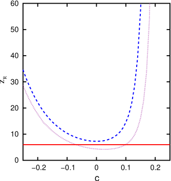
In the case of the running mass model, can become very large even for moderate values of , if , so that the reionization constraint is very powerful. To give a feeling of this strong dependence, we show in Figure 3 the value of as a function of for the simple cases at fixed cosmological parameters.
For each model in the database with a given optical depth we then consider the further prior where the error should take into account the uncertainties due to the different reionization mechanisms.
Finally, we also include a constraint on the variance on a mass scale of of consistent with the limits on the linear power spectrum obtained using measurements of substructure in gravitational lens galaxies in the analysis of dalal .
One should keep in mind that there are many caveats in the inclusion of all above constraints.
We attribute a likelihood to each value of and by marginalizing over the nuisance parameters. We then define our (), confidence levels to be where the integral of the likelihood is () and () of the total value.
III.2 Results
The likelihood contours in the plane obtained analyzing the CMB data under the assumption of a set of “weak” priors (, ) are plotted in Figure 4. As we can see, even if the space of models analyzed is quite broad, the CMB data is able to give strong constraints along the direction. In particular, we obtain the constraint and at c.l… We found that including stronger priors (, ) on the nuisance parameters does not change these results and does not improve significantly the constraints on . Assuming negligible reionization () gives .
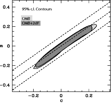
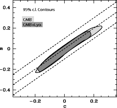
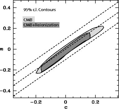
Also plotted in Figure 4 (Top Panel) are the likelihood contours obtained in the combined 2dFGRS-CMB analysis. As we can see, even the inclusion of the 2dF data does not improve significantly the CMB constraints. The combination of the 2dF data is extremely powerful in constraining parameters like and , that define the epoch of equality and the position in the space of the matter spectrum. However, in the CMB+2dF combined analysis, we found at c.l..
In the center panel of Figure 4 we report the likelihood contours obtained in the combined CMB+Ly- analysis. As already noticed by hannestad-run , we find that the Lyman data are able to restrict more strongly the scale dependence of the spectral index and therefore exclude the parameter space at large ; in particular at we have , so that a variation of the spectral index over cosmological scale of the order of 10% is allowed.
Finally, in the bottom panel of Figure 4 we plot the likelihood contours obtained in the combined CMB+reionization analysis. Also in this case part of the region of large is excluded, but still a sizable variation and values of up to 0.2 are allowed. It should be emphasized that this reionization constraint is only one of theoretical consistency. As one can see from Figure 3, the self-consistent value of becomes very large for . If it turns out that , the top part of the allowed region ‘CMB Reionization’ will be excluded.
Focussing on the region ( , ), we plot the likelihood contours in the vs. plane in Figure 5. As we explained before, gives the value of the spectral index on COBE scales, while gives the bend in the spectrum.
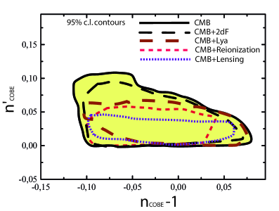
As we can see from the figure, the recent CMB data alone constrains at C.L., while including the constraints from 2dF, Ly-, reionization redshift, limits the amount of deviation from scale invariance to at c.l.. Adding the strong lensing constraint from dalal , as discussed earlier, further constrains at c.l.. It is important to notice that a lower spectral index is consistent with the lensing observation only if . Note also that in all cases the best fit value of is not in the centre of the allowed region, but lower, towards the value . Furthermore, the inclusion of a bend in the power spectrum, does not seem to affect in a considerable way the CMB constraint on since there is a weak correlation between these two variables.
The correlation between and the remaining parameters is investigated in Figure 6 where the likelihood function for is plotted in function of , and the Hubble parameter, .
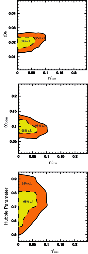
As we can see, the correlation with these parameters is extremely small, meaning that the inclusion of a bending in the primordial spectrum would not drastically affect the actual constraints on the parameters considered. However, an increase in can allow larger (smaller) values of (). The Hubble parameter is poorly constrained by CMB alone.
We have also considered the effect of variations in and on the predicted level of rms mass fluctuations in spheres of . At the moment, there is some sort of tension between the possible values of this parameter obtained from local cluster abundances ( for , see e.g. seljakcluster ) and weak lensing ( for see e.g. refregier ).
In Figure 7 we plot the likelihood contours from the CMB analysis for against (Top Panel) and (Bottom Panel) respectively. As expected, increasing both and increases the level of , but the correlation is not relevant enough to actually detect a bending in the spectrum with present observations.
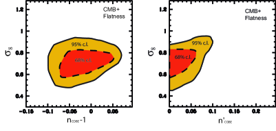
We are in qualitative agreement with other recent constraints on a running spectral index hannestad-run . Precise comparison is difficult mainly because we did not consider a background of gravity waves (that can weaken our final result) since in the running-mass models this is negligible. Furthermore, we considered a more updated CMB dataset respect to the one considered in hannestad-run and we considered different datasets other than CMB. Finally, hannestad-run assumes that can take any value, whereas the running-mass model excludes significantly negative (Eq. (34)). The running-mass model also allows variation of , but this is not very significant at the present level of observation.
We end this discussion of our results by commenting on a recent analysis by Caprini, Hansen and Kunz chk which investigates the variation of that is allowed by observation. First, they assume that the flatness parameter is constant to the end of slow-roll inflation, and taking , they find . The running-mass prediction Eq. (25) for is roughly constant to the end of slow-roll inflation if , and in this regime one needs to have sufficiently close to 1; combining these results gives roughly in agreement with chk . However, chk assume next that instead is roughly constant, and derives a bound . In contrast, the running-mass model predicts which is exponentially large (and of either sign) and strongly varying. Thus the bound on of chk does not apply to the running-mass model in any regime of its parameter space. We remind the reader again that, at the moment, the running-mass model is the only well-motivated model giving significant running of the spectral index.
IV Conclusions
The rather full analysis that we have described confirms the general picture indicated by previous analyses covi . The allowed region in the vs plane depicted in Figure 4 should be compared with the region shown in Figure 2 which approximately delineates the theoretically disfavoured region, and also with the minimum value which is probably needed to generate enough running of the mass even if we go from the Planck scale to . Combining all of these, we see that if is significantly above the minimum value, only the version of the model with and both positive is viable. In that case, the spectral index has significant running which will be detectable in the forseeable future. On the other hand, if is really of order , all choices of the signs of and are possible except maybe negative with positive . Furthermore, if that extreme case can be realized in a viable running-mass model the running of will be so small that it may never be detectable.
Looking at the observational situation in more detail, our results show that the CMB data can put very strong constraints on the value of the spectral index at large scales, , but still allow a pretty large scale-dependence. Other information on the power spectrum, like Lyman data, or strongest assumptions about the reionization epoch are needed to reduce the parameter space in the direction. Still values of of the order of 0.2, and therefore of the order , are allowed. Note also that our allowed region is more or less symmetric under reflection with respect to the line: this means that the present data are not sensitive enough to distinguish the variation of that is predicted by the running-mass model. Finally, we show that the inclusion of the running in the spectral index has a moderate effect on the present CMB determination of the physical matter densities in baryons and cold dark matter .
Acknowledgements It is a pleasure to thank Steen Hansen, Carolina Odman and Joseph Silk for useful comments. We acknowledge the use of CMBFAST sz . AM is supported by PPARC.
References
- (1) E. Torbet et al., Astrophys. J. 521 (1999) L79 [arXiv:astro-ph/9905100]; A. D. Miller et al., Astrophys. J. 524 (1999) L1 [arXiv:astro-ph/9906421].
- (2) P. D. Mauskopf et al. [Boomerang Collaboration], Astrophys. J. 536 (2000) L59 [arXiv:astro-ph/9911444]; A. Melchiorri et al. [Boomerang Collaboration], Astrophys. J. 536 (2000) L63 [arXiv:astro-ph/9911445].
- (3) C. B. Netterfield et al. [Boomerang Collaboration], arXiv:astro-ph/0104460.
- (4) N. W. Halverson et al., arXiv:astro-ph/0104489.
- (5) A. T. Lee et al., Astrophys. J. 561 (2001) L1 [arXiv:astro-ph/0104459].
- (6) T. J. Pearson et al., arXiv:astro-ph/0205388.
- (7) P. F. Scott et al., arXiv:astro-ph/0205380.
- (8) P. de Bernardis et al., [Boomerang Collaboration], arXiv:astro-ph/0105296.
- (9) C. Pryke, N. W. Halverson, E. M. Leitch, J. Kovac, J. E. Carlstrom, W. L. Holzapfel and M. Dragovan, arXiv:astro-ph/0104490.
- (10) R. Stompor et al., Astrophys. J. 561 (2001) L7 [arXiv:astro-ph/0105062].
- (11) X. Wang, M. Tegmark, M. Zaldarriaga, arXiv:astro-ph/0105091.
- (12) J. L. Sievers et al., arXiv:astro-ph/0205387.
- (13) J. A. Rubino-Martin et al., arXiv:astro-ph/0205367.
- (14) A. Lewis and S. Bridle, arXiv:astro-ph/0205436.
- (15) A. Melchiorri and J. Silk, arXiv:astro-ph/0203200.
- (16) C. J. Odman, A. Melchiorri, M. P. Hobson and A. N. Lasenby, arXiv:astro-ph/0207286.
- (17) S. H. Hansen et al., Phys. Rev. D65, 023511 (2002) [arXiv:astro-ph/0105385].
- (18) W. J. Percival et al., arXiv:astro-ph/0105252.
- (19) SDSS collaboration, arXiv:astro-ph/0107417.
- (20) G. Efstathiou et al., arXiv:astro-ph/0109152.
- (21) O. Lahav et al., arXiv:astro-ph/0112162.
- (22) R. Bean and A. Melchiorri, Phys. Rev. D65 041302 (2002) [arXiv:astro-ph/0110472].
- (23) W. J. Percival et al., arXiv:astro-ph/0206256.
- (24) S. Hannestad and E. Mortsell, astro-ph/0205096.
- (25) S. Hannestad, astro-ph/0205223.
- (26) O. Elgaroy et al., Phys. Rev. Lett. 89 061301 (2002).
- (27) D. H. Lyth and A. Riotto, Phys. Rept. 314 1 (1999) [arXiv:hep-ph/9807278].
- (28) A. R. Liddle and D. H. Lyth, “Cosmological Inflation And Large-Scale Structure,” Cambridge, UK: Univ. Pr. (2000) 400 p.
- (29) D. H. Lyth and D. Wands, Phys. Lett. B 524, 5 (2002) [arXiv:hep-ph/0110002]; D. H. Lyth, C. Ungarelli and D. Wands, arXiv:astro-ph/0208055; K. Dimopoulos and D. H. Lyth, arXiv:hep-ph/0209180.
- (30) E. D. Stewart, Phys. Lett. 391B, 34 (1997) [arXiv:hep-ph/9606241].
- (31) E. D. Stewart, Phys. Rev. D56, 2019 (1997) [arXiv:hep-ph/9703232].
- (32) L. Covi, D. H. Lyth and L. Roszkowski, Phys. Rev. D60, 023509 (1999) [arXiv:hep-ph/9809310].
- (33) L. Covi and D. H. Lyth Phys. Rev. D59, 063515 (1999) [arXiv:hep-ph/9809562].
- (34) L. Covi Phys. Rev. D60, 023513 (1999) [arXiv:hep-ph/9812232].
- (35) G. German, G. Ross and S. Sarkar, Phys. Lett. 469B, 46 (1999) [arXiv: hep-ph/9908380].
- (36) D.H. Lyth and L. Covi, Phys. Rev. D62 103504 (2000) [arXiv:astro-ph/0002397].
- (37) L. Covi and D. H. Lyth, MNRAS, Vol. 326, 885-893 (2001) [arXiv:astro-ph/0008165].
- (38) S. Hannestad, S.H. Hansen and F.L. Villante, Astropart. Phys. 16, 137-144 (2001) [arXiv:astro-ph/0012009]; S. Hannestad, S.H. Hansen, F.L. Villante and A.J.S. Hamilton, Astropart. Phys. 17, 375-382 (2002) [arXiv:astro-ph/0103047].
- (39) L. Randall, M. Soljacic and A. H. Guth, Nucl. Phys. B 472, 377 (1996) [arXiv:hep-ph/9512439].
- (40) U. Seljak and M. Zaldarriaga, Astrophys. J. , 469, 437 (1996) [arXiv:astro-ph/9603033].
- (41) N. Gnedin, arXiv:astro-ph/0110290.
- (42) N. Aghanim, P. G. Castro, A. Melchiorri and J. Silk, arXiv:astro-ph/0203112.
- (43) S. L. Bridle, R. Crittenden, A. Melchiorri, M. P. Hobson, R. Kneissl and A. N. Lasenby, arXiv:astro-ph/0112114.
- (44) M. Tegmark, A.J.S. Hamilton, Y. Xu, arXiv:astro-ph/0111575.
- (45) R. A. Croft et al., arXiv:astro-ph/0012324.
- (46) N. Dalal and C.S. Kochanek, arXiv:astro-ph/0202290.
- (47) U. Seljak, arXiv:astro-ph/0111362.
- (48) A. Refregier et al., arXiv:astro-ph/0203131.
- (49) C. Caprini, S. H. Hansen and M. Kunz, arXiv:hep-ph/0210095.