W-Particle Distribution in ElectroWeak Tachyonic Pre-Heating

Abstract

Results are presented of a numerical study of the distribution of W-bosons generated in a tachyonic electroweak pre-heating transition.

1 W-distribution in tachyonic electroweak baryogenesis

The electroweak transition may have taken place shortly after inflation ending at a low energy scale, and this possibility has been used to suggest alternative scenarios for baryogenesis. We have studied such a transition in the SU(2)-Higgs model with effective CP-violation [1]. The transition is assumed to have taken place at zero temperature. In the quenching approximation, it is induced simply by flipping the sign of the quadratic term in the Higgs potential, $\mu^{2}\phi^{\dagger}\phi\to-\mu^{2}\phi^{\dagger}\phi$. This causes the Higgs field to go through a spinodal instability in which its particle numbers initially grow exponentially fast, leading to classical behavior [2, 3, 4, 5, 6, 7]. The gauge fields react strongly, and it is interesting to see the emergence of effective W-particles, their energy spectrum $\omega_{k}$, and their distribution function $n_{k}$.

The numerical simulation is carried out in the temporal gauge $A_{0}=0$. To define $\omega_{k}$ and $n_{k}$, we transform to the Coulomb gauge $\partial_{j}A_{j}=0$ (which is a smooth gauge in which it makes sense to Fourier transform to momentum space), and maximally coarse-grain the equal-time correlators of the gauge field and its canonical conjugate ($E_{j}$) over the (periodic) volume $L^{3}$,

$$\frac{1}{3L^{3}}\int d^{3}z\,\langle A^{p}_{i}({\bf x}+{\bf z})A^{p}_{j}({\bf y}+{\bf z})\rangle = C^{AA}_{ij}({\bf x}-{\bf y}),$$

$$\frac{1}{3L^{3}}\int d^{3}z\,\langle E^{p}_{i}({\bf x}+{\bf z})E^{p}_{j}({\bf y}+{\bf z})\rangle = C^{EE}_{ij}({\bf x}-{\bf y}),$$

where we also averaged over the three isospin directions. After Fourier transformation, averaging over the transverse modes,

$$\frac{1}{2}\delta_{ij}\int d^{3}x\,e^{-i{\bf k}\cdot{\bf x}}\,C^{AA}_{ij}({\bf x}) = C^{AA}_{\bf k},$$

$$\frac{1}{2}\left(\delta_{ij}-\hat{k}_{i}\hat{k}_{j}\right)\int d^{3}x\,e^{-i{\bf k}\cdot{\bf x}}\,C^{EE}_{ij}({\bf x}) = C^{EE}_{\bf k},$$

and averaging over directions, ${\bf k}\to k=|{\bf k}|$, the time-dependent particle spectrum and distribution function is obtained by solving

$$C^{AA}_{k}=n_{k}/\omega_{k}\;\;\;\;\;\;\;\;\;\;\;\;C^{EE}_{k}=n_{k}\omega_{k}$$

for $n_{k}$ and $\omega_{k}$. Note that $n_{k}$ appears and not $n_{k}+1/2$, since we are using the classical approximation.

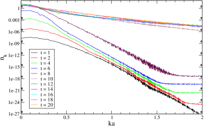
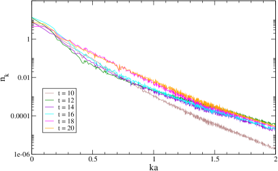
Figure 1: $n_{k}$ versus $ak$ at early times. Time is in units of $m_{H}^{-1}$ and the quench is at $t=0$.

We present here results obtained from only one gauge field configuration, i.e. the average over initial conditions $\langle\cdots\rangle$ is not carried out. If classical behavior applies, then one field configuration corresponds to one realized universe. Of course, statistical observables such as $n_{k}$ and $\omega_{k}$ will suffer from ‘cosmic variance’, which may be severe in a small volume. The parameters of the simulation on a lattice of $60^{3}$ sites are given by

couplings: $$g^{2}=4/9,\;\;\;1=8\lambda/g^{2}=m_{H}^{2}/m_{W}^{2}$$

physical size $$L=21\,m_{H}^{-1},\;\;\;\mbox{lattice spacing}\;\;a=0.35\,m_{H}^{-1}$$

Figure 1 shows $n_{k}$ at early times after the quench at $t=0$. We see an exponential growth of the low momentum modes until they saturate around $t\approx 8\,m_{H}^{-1}$, after which the tail quickly acquires a different slope on the log-plot.

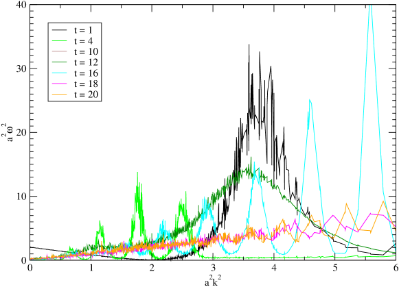
Figure 2: $a^{2}\omega_{k}^{2}$ versus $a^{2}k^{2}$ at early times. The particle interpretation starts to make sense from $tm_{H}\approx 18$ onwards.

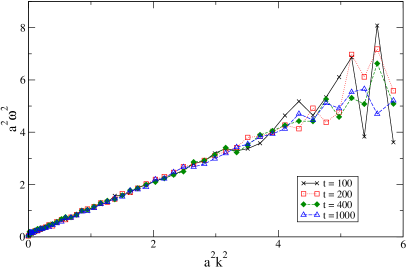
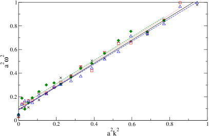
Figure 3: $a^{2}\omega_{k}^{2}$ versus $a^{2}k^{2}$ at later times. The fitted slopes are 1 within a few percent. The fitted intercepts correspond to effective masses $m_{\rm eff}/m_{H}\approx 0.86$, 0.88, 0.95, 0.85 respectively for $tm_{H}=100$, 200, 400, 1000.

Figure 2 shows $\omega_{k}$ for $t\leq 20\,m_{H}^{-1}$. It suffers greatly from fluctuations (‘cosmic variance’ in our small ‘universe’), and we averaged the data in bins of size $\Delta|{\bf k}|\approx 0.14\,m_{H}$. Only from $t=18\,m_{H}^{-1}$ onwards a sensible $\omega_{k}$ emerges, as can also be seen at later times in Figure 3. The spectrum is close to the simple form $\omega_{k}^{2}=m_{\rm eff}^{2}+k^{2}$ (on the lattice we use $k^{2}\to a^{-2}\sum_{j}[2-2\cos(ak_{j})]$), with $m_{\rm eff}\approx m_{W}$, the zero-temperature input-value.

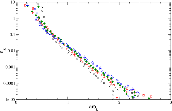
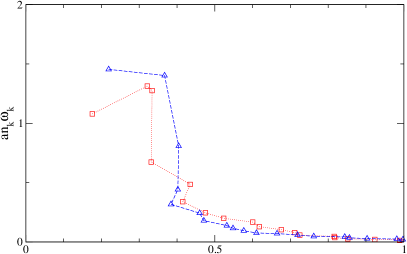
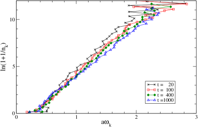
Figure 4: $n_{k}$ (top), $n_{k}\omega_{k}a$ (bottom left) and $\ln(1+1/n_{k})$ (bottom right) versus $\omega_{k}a$, at times $tm_{H}=20$, 100, 400, 1000.

At later times $20\leq tm_{H}\leq 1000$ the distribution $n_{k}$ does not change much, as can be seen in Figure 4. At $k=0$, the particle number stays roughly constant, $6\lesssim n_{0}\lesssim 7$, while the tail of the distribution appears to rise slowly. There is little power beyond $a\omega_{k}=am_{H}=0.35$ (top plot).

The data do not yet show clear signs of classical equilibration, $n_{k}\to T/\omega_{k}$. One expects a plateau to develop in $n_{k}\omega_{k}$, but the ‘plateau’ in the lower-left plot does not look very convincing yet as it involves only two $k$-values.

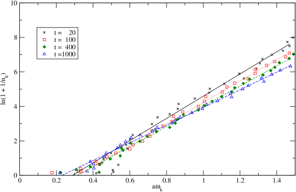
Figure 5: Linear fits $\ln(1+1/n_{k})\approx(\omega_{k}-\mu)/T$ resulting in an effective temperature $T/m_{H}=0.44$, 0.46, 0.49, 0.56, and effective chemical potential $\mu/m_{H}=0.8$, 0.9, 0.9, 0.7, respectively for $tm_{H}=20$, 100, 400 and 1000.

The lower-right plot in Figure 4 shows $\ln(1+n_{k}^{-1})$, which for a Bose-Einstein distribution would have the linear form $(\omega_{k}-\mu)/T$. The data are roughly compatible with this behavior, the fits in Figure 5 indicate an effective temperature that slowly increases as the higher momentum modes get more occupied, $T/m_{H}=0.44\to 0.56$, with a hint of a decreasing effective chemical potential $\mu\approx 0.8\to 0.7$, as $t$ increases from 20 to 1000 $m_{H}^{-1}$.

2 Conclusion

After $t\approx 20\,m_{H}^{-1}$, the particles produced by the instability settle into an effective temperature of about $0.5\,m_{H}$. Subsequent evolution is slow in the SU(2)-Higgs model, in the classical approximations used here: the modes are massive and the effective interactions appear to be weak at the BE-temperature $T\approx 0.5\,m_{H}$. The Higgs particles have roughly the same effective temperature.

The initial conditions for this simulation do not put power into the high-momentum modes near the cutoff [1, 3]. There is furthermore little draining of power from the low- to high-momentum modes, so Rayleigh-Jeans effects are negligible. Lattice artefacts are also under control, since the distribution function drops exponentially fast and there is little power in the gauge-field modes beyond $ak=0.5$. In particular, it makes sense to use a simple lattice version [1] of an effective CP-violating term $\kappa\mbox{Tr}\,\phi^{\dagger}\phi F_{\mu\nu}\tilde{F}^{\mu\nu}$ in the lagrangian.

Acknowledgments.
This work was supported in part by FOM.

References

- [1] A. Tranberg, J. Smit, Chern-Simons number asymmetry from CP violation during tachyonic preheating, contribution to this workshop.
- [2] G. N. Felder, J. García-Bellido, P. B. Greene, L. Kofman, A. D. Linde and I. Tkachev, Phys. Rev. Lett. 87 (2001) 011601 [arXiv:hep-ph/0012142].
- [3] M. Sallé, J. Smit, and J. C. Vink, in proceedings Cosmo 01, arXiv:hep-ph/0112057; Nucl. Phys. (Proc. Suppl.) 106 (2002) 540, hep-lat/0110093.
- [4] J. García-Bellido and E. Ruiz Morales, Phys. Lett. B 536 (2002) 193 [arXiv:hep-ph/0109230].
- [5] E. J. Copeland, S. Pascoli and A. Rajantie, Phys. Rev. D 65 (2002) 103517 [arXiv:hep-ph/0202031].
- [6] J. García-Bellido, M. García-Pérez, A. Gonzáles-Arroyo, hep-ph/0208228.
- [7] Sz. Borsányi et al., contribution to this workshop.