Quantitative evolution of global strings from the Lagrangian viewpoint

Abstract

We clarify the quantitative nature of the cosmological evolution of a global string network, that is, the energy density, peculiar velocity, velocity squared, Lorentz factor, formation rate of loops, and emission rate of Nambu-Goldstone bosons, based on a new type of numerical simulation of scalar fields in Eulerian meshes. We give a detailed explanation of a method to extract the above-mentioned quantities to characterize string evolution by analyzing scalar fields in Eulerian meshes from a Lagrangian viewpoint. We confirm our previous claim that the number of long strings per horizon volume in a global string network is smaller than in the case of a local string network by a factor of $\sim$10 even under cosmological situations, and its reason is clarified.

I Introduction

The idea of spontaneous symmetry breaking in high energy physics has profound implications on the vacuum structure of the Universe and our Universe has presumably experienced various phase transitions, which are thermal Kibble or nonthermal KVY . Their consequences may be traced by topological defects that may have been produced with them. Indeed, many implications of topological defects for cosmology have been investigated VS . Furthermore, recently, defect formations have also been discussed in the context of phase transitions which occur in the laboratory. For example, defect formations in ³He He3 and ⁴He He4 are studied in detail. Thus the cosmological scenario of defect formation can be tested by experiments in the laboratory Zurek .

Among several types of topological defects, strings hold a unique position in cosmology, because they do not overclose the Universe, unlike magnetic monopoles or domain walls, settling down to a scaling solution in which the typical scale of the network grows in proportion to the horizon scale Kibble ; Kibble2 . The key mechanism to achieve a scaling behavior is intercommutation of infinite strings to dissipate their energy by producing closed loops, which subsequently decay to radiation of relativistic particles or gravitational waves depending on their property. While one may understand the qualitative nature of the scaling solution analytically, more quantitative features such as the number of long strings per horizon volume or the size spectrum of loops produced cannot be obtained unless full numerical analyses are performed.

Although there exist two types of strings, namely, local and global strings depending on the nature of the symmetry breaking, only the former have been investigated extensively for a long time as far as numerical analysis is concerned. By numerically solving the equation of motion of string segments derived from the Nambu-Goto action NG , several groups have confirmed the scaling behavior AT ; AT2 ; BB ; AS , and estimated the scaling parameter $\xi$ as $\xi\simeq 10$ in the radiation dominated universe AT2 ; BB ; AS . Here, $\xi$ is defined as

$$\xi=\rho_{\infty}t^{2}/\mu$$ (1)

where $\rho_{\infty}$ is the energy density of long strings and $\mu$ is the string tension per unit length. Thanks to this feature, local strings generate density fluctuations with a scale-invariant spectrum and their cosmological consequences were investigated extensively some time ago. Recent observations of the cosmic microwave background anisotropy cmb , however, disfavor the cosmic-string scenario of structure formation, and the motivations to investigate local strings as a source of primordial density fluctuations have somewhat diminished, although a hybrid model of structure formation may still be viable, where primordial fluctuations are comprised of adiabatic fluctuations induced by inflation and isocurvature perturbations by topological defects TDCMB .

On the other hand, global strings are much better motivated in the context of axion cosmology. They are formed as a consequence of the breaking of the Peccei-Quinn U(1) symmetry PQ ; VE , which was introduced to solve the strong $CP$ problem in quantum chromodynamics. These global strings radiate axions as associated Nambu-Goldstone (NG) bosons Davis , which are one of the most promising candidates for cold dark matter. Despite their importance, the cosmological evolution of global strings has been less studied and the results of local strings have often been borrowed even though there is a decisive difference between them. For local strings, the gradient energy of scalar fields is canceled out by gauge fields far from the core. The string core is well localized and the false vacuum energy of the core dominates the system. Hence the Nambu-Goto action is suitable as an effective action in order to study the cosmological evolution of local strings except at crossing NG . On the other hand, for global strings, there are no gauge fields to cancel the gradient energy of the NG scalar field, which dominates over the false vacuum energy of the core. The effective action appropriate for global strings is not the Nambu-Goto action but the Kalb-Ramond action, which incorporates NG bosons and their couplings with the core KR . Also, due to the gradient energy of the NG scalar field, a long-range force works between global strings. Thus, the behavior of the two types of string is expected to be different and it is nontrivial whether global strings relax to a scaling regime. In fact, for example, the behavior of global monopoles is quite different from that of local monopoles due to long-range forces. While the former may be useful in cosmology monopole ; Yamaguchi , the latter causes a disaster Preskill unless diluted by inflation. Furthermore, it has been shown in the literature that local and global strings behave differently in two dimensional space YB ; 2dim .

There have been several attempts to investigate the cosmological evolution of the global string network by use of the Kalb-Ramond action BS ; sharp . However, the Kalb-Ramond action is too complicated to be dealt with numerically. It has difficulty because of logarithmic divergence due to the self-energy of the string. In such a situation the authors and Kawasaki made the first numerical investigations of the cosmological evolution of global strings without resort to the Kalb-Ramond action. We instead solved the equations of motion for scalar fields forming strings in three dimensional Eulerian meshes YKY . We found that the global string network would also go into a scaling regime but the scaling parameter $\xi$ was found to be of the order of unity YKY ; YYK , which is significantly smaller than the case of local strings ($\xi\simeq 10$).

Recently, however, this quantitative difference was questioned and it was claimed that the smallness of the scaling parameter of global strings might be a fake due to the small dynamic range of the numerical simulations MS ; MSM . The authors of MS ; MSM claimed that in our simulations global strings lost their energy by excessive direct emission of NG bosons. Based on the speculation that such direct emission of NG bosons from long strings would be negligible on cosmological scales, they reached a conjecture that both types of strings behave quantitatively in the same way in the cosmological context, namely, $\xi\simeq 10$, with the only difference between them being the energy loss mechanism of closed loops.

In order to clarify the evolution of global strings on cosmological scales, we should first study which is the dominant energy loss mechanism of long strings in numerical simulations, loop production or direct emission of NG bosons. We note that the master equation for the energy density of long strings, $\rho_{\infty}$, can be expressed as

$$\frac{d\rho_{\infty}}{dt}=-2H(1+\left\langle v^{2}\right\rangle)\rho_{\infty}-\Gamma_{\rm loop}\rho_{\infty}-\Gamma_{\rm NG}\rho_{\infty},$$ (2)

where the second and the third terms on the right-hand side represent energy loss due to loop formation and direct emission of NG bosons or axions, respectively, and $\left\langle v^{2}\right\rangle$ denotes the average square velocity of string segments. For our purpose, we need to calculate both the loop production rate $\Gamma_{\rm loop}$ and the emission rate of NG bosons $\Gamma_{\rm NG}$, and compare their magnitudes in simulations.

If the system relaxes to the scaling regime, which will be confirmed to be the case shortly, the string network is described by the so-called one-scale model with the characteristic scale $L\equiv\sqrt{\mu/\rho_{\infty}}$, which grows with the horizon scale $L\propto t$. If we introduce the loop production coefficient $c$ and the emission coefficient $\kappa$ of the NG bosons by

$$\Gamma_{\rm loop}\rho_{\infty}=c\frac{\rho_{\infty}}{L},~{}~{}~{}~{}~{}\Gamma_{\rm NG}\rho_{\infty}=\kappa\frac{\rho_{\infty}}{L},$$ (3)

these parameters remain constant in the one-scale picture and are related to the scaling parameter $\xi$ as

$$\xi=\left(\frac{1-\left\langle v^{2}\right\rangle}{c+\kappa}\right)^{2}.$$ (4)

Indeed, if $\kappa$ incorrectly turned out to be much larger than $c$, we would find a smaller value of $\xi$ than it should really be. Hence, it is essential to evaluate the parameters $c$ and $\kappa$ in the scaling regime.

In our previous simulations YKY , however, it was impossible to calculate these quantities for two reasons. First, in the previous work a lattice was identified as part of a string based on the value of the potential energy there, which had the microscopic problem that we occasionally found disconnected string pieces, although the overall features were traced reasonably well. Second, it was impossible to monitor intercommutation of strings for lack of dynamical information, namely, the velocity of each string segment. These problems are overcome by our new identification scheme and Lagrangian analysis of the evolution of strings YY .

The rest of the paper is organized as follows. In Sec. II we present the method of our new procedure to follow the Lagrangian evolution of global strings in Eulerian simulations, that is, new methods of identification of strings, measurement of string velocity, and estimation of the intercommutation rate. In Sec. III the results are described and applied to cosmological situations. Finally, Sec. IV is devoted to a discussion and conclusion.

II numerical simulations

II.1 Formulation

We consider the following Lagrangian density for two-component real scalar fields $\phi_{a}(x)$ ($a=1,2$) which can accommodate global strings:

$${\cal L}[\phi_{a}]=\frac{1}{2}g_{\mu\nu}(\partial^{\mu}\phi_{a})(\partial^{\nu}\phi_{a})-V[\phi_{a},T],$$ (5)

in the spatially flat Robertson-Walker spacetime,

$$ds^{2}=g_{\mu\nu}dx^{\mu}dx^{\nu}=dt^{2}-R^{2}(t)d\mbox{\boldmath${x}$}^{2},$$ (6)

with $R(t)$ being the scale factor. We adopt the following potential at finite temperature $T$:

$$V[\phi_{a},T] = \frac{\lambda}{4}(\phi^{2}-\sigma^{2})^{2}+\frac{\lambda}{6}T^{2}\phi^{2}$$ (7)

$$= \frac{\lambda}{4}(\phi^{2}-\eta^{2})^{2}+\frac{\lambda}{4}(\sigma^{4}-\eta^{4}).$$ (8)

Here $\phi^{2}\equiv\phi_{1}^{2}+\phi_{2}^{2}$ and $\eta^{2}\equiv\sigma^{2}-T^{2}/3=\sigma^{2}(1-T^{2}/T_{c}^{2})$ with $T_{c}\equiv\sqrt{3}\sigma$ being the critical temperature. Below the critical temperature, global U(1) symmetry is broken to form global strings.

The equations of motion for the scalar fields are given by

$$\ddot{\phi_{a}}(x)+3H(t)\dot{\phi_{a}}(x)-\frac{1}{R(t)^{2}}\nabla^{2}\phi_{a}(x)+\frac{\partial V}{\partial\phi_{a}}=0,$$ (9)

where an overdot represents the time derivative. The discretization of these differential equations is given in Appendix A. Our numerical calculations are based on the staggered leapfrog method with second order accuracy both in time and in space. In the radiation dominated Universe, the Hubble parameter $H(t)=\dot{R}(t)/R(t)$ and cosmic time $t$ are given by

$$H(t)^{2}=\frac{8\pi}{3M_{Pl}^{2}}\frac{\pi^{2}}{30}g_{*}T^{4},~{}~{}~{}~{}~{}t=\frac{1}{2H}\equiv\frac{\epsilon}{T^{2}},$$ (10)

where $M_{Pl}=1.2\times 10^{19}$ GeV is the Plank mass and $g_{*}$ is the total number of degrees of freedom for the relativistic particles. We define a dimensionless parameter $\zeta$ as

$$\zeta\equiv\frac{\epsilon}{\sigma}=\left(\frac{45M_{Pl}^{2}}{16\pi^{3}g_{*}\sigma^{2}}\right)^{1/2},$$ (11)

and take $\zeta=10$ and the self-coupling $\lambda=0.08$ for definiteness, but these particular choices do not affect the results. We start the numerical simulation at the temperature $T_{i}=2T_{c}$ corresponding to $t_{i}=t_{c}/4$ and adopt as an initial condition the thermal equilibrium state with a mass equal to the inverse curvature of the potential at that time. In this state $\phi_{a}$ and $\dot{\phi}_{a}$ are Gaussian distributed with the correlation functions

$$\left\langle\beta|\phi_{a}(\mbox{\boldmath${x}$})\phi_{b}(\mbox{\boldmath${y}$})|\beta\right\rangle_{\rm equal~{}time} = \int\frac{d^{3}k}{(2\pi)^{3}}\frac{1}{2\sqrt{\mbox{\boldmath${k}$}^{2}+m^{2}}}\coth{\frac{\beta\sqrt{\mbox{\boldmath${k}$}^{2}+m^{2}}}{2}}e^{i\mbox{\boldmath${k}$}\cdot(\mbox{\boldmath${x}$}-\mbox{\boldmath${y}$})}\delta_{ab}\>,$$ (12)

$$\langle\beta|\dot{\phi}_{a}(\mbox{\boldmath${x}$})\dot{\phi}_{b}(\mbox{\boldmath${y}$})|\beta\rangle_{\rm equal~{}time} = \int\frac{d^{3}k}{(2\pi)^{3}}\frac{\sqrt{\mbox{\boldmath${k}$}^{2}+m^{2}}}{2}\coth{\frac{\beta\sqrt{\mbox{\boldmath${k}$}^{2}+m^{2}}}{2}}e^{i\mbox{\boldmath${k}$}\cdot(\mbox{\boldmath${x}$}-\mbox{\boldmath${y}$})}\delta_{ab}\>,$$ (13)

where $m^{2}=V^{\prime\prime}[\phi_{a},T_{i}]$ and $\beta=T^{-1}_{i}$. $\phi_{a}(\mbox{\boldmath${x}$})$ and $\dot{\phi}_{a}(\mbox{\boldmath${y}$})$ are uncorrelated for $\mbox{\boldmath${x}$}\neq\mbox{\boldmath${y}$}$. We generate the initial configuration in the momentum space, where the scalar fields are uncorrelated. Then they are transformed into the position space by fast Fourier transformation.

We perform simulations in five different sets of lattice sizes and spacings as shown in Table 1 to investigate their effects on the results. In all cases, the time step is taken as $\Delta t=0.01t_{i}$, and the periodic boundary condition is adopted. In the case (a), the box size is nearly equal to the horizon length $H^{-1}$ and the lattice spacing to the typical core width $\delta\sim 1.0/(\sqrt{2\lambda}\sigma)$ of a string at the final time $t_{f}=200t_{i}$. The other cases have equal or larger simulation volumes.

In this type of numerical calculation, it is a nontrivial task to identify string cores from the data of scalar fields because a point with $\phi_{a}=0$ corresponding to a string core is not necessarily situated at a lattice point. So, in the next subsection, we give our new method of identification of string cores.

II.2 Identification method of strings

In previous work YKY ; YYK , whether a lattice point was a part of string core was judged based on the potential energy density there. That is, a lattice point was identified to be at the core of a string if the potential energy density there was found to be larger than that of a static cylindrically symmetric solution of a global string at $r=\Delta x_{\rm phys}/\sqrt{2}$ off center, where $\Delta x_{\rm phys}$ is the physical length of the lattice spacing at each time.

Although this method worked fairly well to evaluate the scaling parameter, it was inadequate to fully identify strings particularly for small loops which do not resemble the static cylindrically symmetric solution due to the curvature. As a result we occasionally found disconnected string segments that should not exist in reality. Furthermore, it was impossible to find a more correct position of the string core in a box beyond the lattice spacing, which is extremely important to evaluate the length and velocity of the string correctly.

Here we develop a new method of string identification based on the fact that strings lie on the intersection of two surfaces $\phi_{1}(\mbox{\boldmath${x}$},t)=0$ and $\phi_{2}(\mbox{\boldmath${x}$},t)=0$, so that if a string penetrates a (sufficiently small) plaquette, $\phi_{a}$ has a different sign at one or two corners of the plaquette from the rest for each $a$. First, we classify the relative phase of the scalar fields into three groups as shown in Fig. 1 (left), that is,

$$\theta\equiv\arccos\frac{\phi_{2}}{\sqrt{\phi_{1}^{2}+\phi_{2}^{2}}}+2\pi\left[1-\Theta(\phi_{2})\right],$$ (14)

$${\rm(i)} \quad 0\leq\theta<\frac{\pi}{2},$$

$${\rm(ii)} \quad\frac{\pi}{2}\leq\theta<\frac{3\pi}{2},$$ (15)

$${\rm(iii)} \quad\frac{3\pi}{2}\leq\theta<2\pi,$$

where the arccosine should take the principal value and $\Theta(\phi_{2})$ is the step function.

Then, we judge whether a string penetrates a plaquette by monitoring the phase rotation around it just as in the Vachaspati-Vilenkin algorithm VV . If we assigned an equal range $2\pi/3$ of the relative phase to all regions (i)-(iii) as in the original Vachaspati-Vilenkin algorithm and judged the presence of a string from the phase rotation, we would occasionally identify a plaquette as containing a string even if $\phi_{1}$ or $\phi_{2}$ takes the same sign at its four corners. This is the main reason why all regions (i)-(iii) do not have equal ranges of the relative phase $\theta$ in our scheme, in which this case is avoided and $\phi_{a}$ takes a different sign for each $a$ at one or two corners of each plaquette along which a circular phase rotation is observed. Then, using the values of $\phi_{a}$ at its four corners we can draw two lines corresponding to $\phi_{1}=0$ and $\phi_{2}=0$ and their intersection is identified with the point where a string penetrates the plaquette, as shown in Fig. 2.

In fact, the intersection point could be found outside the plaquette. In this case, the nearest point on the edge of the plaquette from the intersection is identified as the position of the string as shown in Fig. 3. In our simulations we encountered such a case very rarely and it did not cause any serious problems.

By joining these points, the strings are completely connected and a more accurate total length of the global string can be obtained. One may wonder if our biased classification of the relative phase may cause some artificial effects on the result of numerical simulations. So we have tried another classification of the relative phase as shown in Fig. 1 (right), that is,

$${\rm(i)} \quad 0\leq\theta<\frac{\pi}{2},$$

$${\rm(ii)} \quad\frac{\pi}{2}\leq\theta\leq\pi,\quad$$ (16)

$${\rm(iii)} \quad\pi\leq\theta<2\pi,$$

and confirmed that the results do not depend on the classification scheme for the relative phase.

At each time step, we can evaluate the total length of the global string by the method shown above. Since strings typically move at a speed close to unity, we should multiply the length of each string segment by $\mu=\gamma\mu_{s}$ to calculate the total energy density of strings. Here $\gamma$ is the Lorentz factor and $\mu_{s}\simeq 2\pi\eta^{2}\ln\left[t/(\delta\xi^{1/2})\right]$ is the line density of a static string MSM . So it is important to establish a method to calculate the velocity and Lorentz factor of the string segments, which will be presented shortly. We can then evaluate the scaling parameter $\xi$ from Eq. (1).

II.3 Velocity of strings

Here we describe our method to evaluate the velocity of strings, which is a nontrivial task in Eulerian calculations of scalar field configurations.

First we expand the scalar fields $\phi_{a}(\mbox{\boldmath${x}$},t_{0}+\delta t)$ around $\phi_{a}(\mbox{\boldmath${x}$}_{0},t_{0})$ up to first order,

$$\phi_{a}(\mbox{\boldmath${x}$},t_{0}+\delta t)\cong\phi_{a}(\mbox{\boldmath${x}$}_{0},t_{0})+\nabla\phi_{a}(\mbox{\boldmath${x}$}_{0},t_{0})\cdot(\mbox{\boldmath${x}$}-\mbox{\boldmath${x}$}_{0})+\dot{\phi}_{a}(\mbox{\boldmath${x}$}_{0},t_{0})\delta t\qquad(a=1,2).$$ (17)

Suppose that a string core exists at a point $\mbox{\boldmath${x}$}_{0}$ at time $t_{0}$ and moves to a point ${x}$ at $t=t_{0}+\delta t$, that is, $\phi_{a}(\mbox{\boldmath${x}$}_{0},t_{0})=0$ and $\phi_{a}(\mbox{\boldmath${x}$},t_{0}+\delta t)=0$ for each $a$. Then, from Eq. (17) we find that the loci of the string core at $t=t_{0}+\delta t$ lie on the intersection of two planes,

$$\nabla\phi_{a}(\mbox{\boldmath${x}$}_{0},t_{0})\cdot(\mbox{\boldmath${x}$}-\mbox{\boldmath${x}$}_{0})+\dot{\phi}_{a}(\mbox{\boldmath${x}$}_{0},t_{0})\delta t=0,$$ (18)

with $a=1,2$. Since motion tangential to a string is a gauge mode, we should evaluate the velocity normal to it. Suppose that the line normal to the string segment at $(\mbox{\boldmath${x}$}_{0},t_{0})$ reaches across the above intersection line at $\mbox{\boldmath${x}$}=\mbox{\boldmath${x}$}_{l}(\mbox{\boldmath${x}$}_{0},t_{0},\delta t)$. Then we can easily obtain the velocity of this string segment as

$$\mbox{\boldmath${v}$}(\mbox{\boldmath${x}$}_{0},t_{0}) = \lim_{\delta t\longrightarrow 0}\frac{\mbox{\boldmath${x}$}_{l}(\mbox{\boldmath${x}$}_{0},t_{0},\delta t)-\mbox{\boldmath${x}$}_{0}}{\delta t}$$ (19)

$$= \left.\frac{\dot{\phi}_{1}\nabla\phi_{2}-\dot{\phi}_{2}\nabla\phi_{1}}{|\nabla\phi_{1}\times\nabla\phi_{2}|}\right|_{\mbox{\boldmath${x_{0}}$},t_{0}}.$$

We calculate the velocity at each point where the strings cross plaquettes. For this purpose we need to evaluate $\dot{\phi}_{a}$ and $\nabla\phi_{a}$ at arbitrary points on a plaquette, as shown explicitly in Appendix B, where $\dot{\phi}_{a}$ and $\nabla\phi_{a}$ are given by the quantities on lattice points up to the second order. Collecting the value of Eq. (19) at each intersection of strings with plaquettes, we can obtain the average of the velocity, the velocity squared, and the Lorentz factor.

II.4 Intercommutation of strings

Now we discuss the energy loss rate from infinite strings to loops by calculating the intercommutation rate $c$. In simulations of cosmic strings based on the Nambu-Goto action, one has to assign the intercommutation probability of intersecting strings by hand due to the lack of microscopic information. Since the strings are identified from the scalar field configuration in our simulation, we can unambiguously calculate how strings intersect with each other, namely, whether they simply pass through or intercommute upon collision. We can therefore identify new loops by monitoring the lengths of all long strings and loops at each time step and comparing the data with those at the previous time step.

II.5 NG boson emission

It is very difficult to directly evaluate the NG boson emission rate because separation of the emitted axions and NG phase associated with the string core is nontrivial. Since loops also emit these particles, it is a formidable task to identify axions radiated from long strings only. However, we have already described how we can obtain $\rho_{\infty}$, $\langle v^{2}\rangle$, and $\Gamma_{\rm loop}$ from simulation data at each time step, and $d\rho_{\infty}/dt$ can also be calculated from $\rho_{\infty}$ at two adjacent time steps. So all the quantities in the master equation (2) can be calculated from our simulation data except for the last term, which can be found from the equation itself. In particular, in the scaling regime, when the one-scale description suffices, we can find $\kappa$ from

$$\kappa=\frac{1-\left\langle v^{2}\right\rangle}{\sqrt{\xi}}-c.$$ (20)

III Results

III.1 Scaling parameter

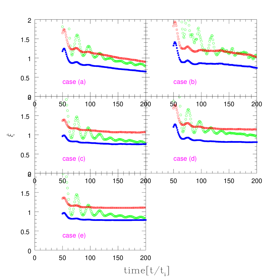
Figure 4: Time evolution of the scaling parameter $\xi$. Filled squares represent our new identification method. Blank circles correspond to our previous identification method based on the potential energy density YKY ; YYK . Blank squares are results of the Vachaspati-Vilenkin algorithm.

In Fig. 4, the time evolution of $\xi$ is depicted for all cases [(a)-(e)]. The filled squares represent the time development of $\xi$ for the new identification method. For comparison, the results of our previous identification method based on the potential energy density YKY ; YYK , which slightly overestimates $\xi$ by a factor of $1.2$, are shown by blank circles. The results of the original Vachaspati-Vilenkin identification scheme are indicated by blank squares, obtained by counting the number of boxes through which a string passes as was done in Ref. MSM . This method overestimates $\xi$ by a factor of $1.4$.

We find that differences in the simulation settings except the box size normalized by the final horizon scale do not affect the overall behavior significantly. $\xi$ becomes smaller in the smallest box size with $=H^{-1}$ at the final time. This is mainly because under the periodic boundary conditions, a string feels an attractive force from the boundary and tends to disappear. Indeed, in the case (a) this artificial effect starts to operate before the system really relaxes to the scaling solution, so $\xi$ continues decreasing without a plateau. On the other hand, in the case (b), the boundary effect becomes operative after $t\simeq 130$ when $\xi$ starts to decrease from the scaling value. The other three cases, whose box size is larger than $2H^{-1}$, are free from the boundary effects and the scaling parameter $\xi$ remains constant. Hence we conclude that after the relaxation period the global string network goes into the scaling regime. From Table 2, which shows average values of $\xi$ after some relaxation period ($t>80$), $\xi$ is found to be $\xi\simeq 0.80$ in the scaling regime.

III.2 String velocity

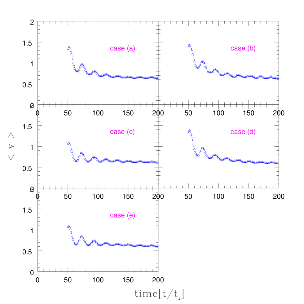
Figure 5: Time evolution of average velocity of global strings is shown.

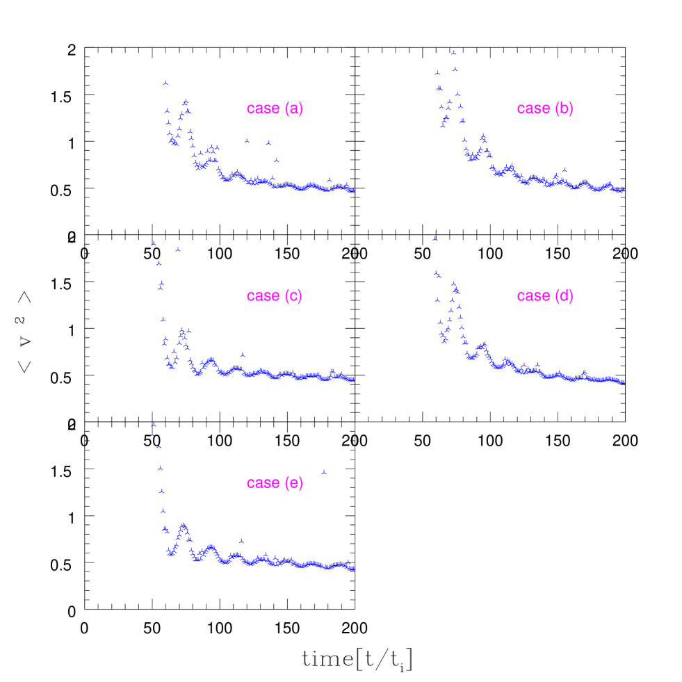
Figure 6: Time evolution of average square velocity.

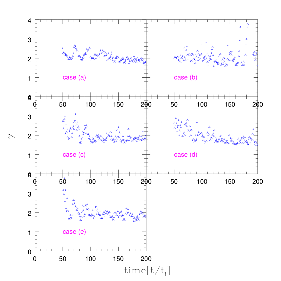
Figure 7: Time evolution of average Lorentz factor.

In Figs. 5 – 7, the time evolutions of the average velocity $\left\langle v\right\rangle$, the average square velocity $\left\langle v^{2}\right\rangle$, and the Lorentz factor $\left\langle\gamma\right\rangle$ are shown. After some relaxation period, they become fairly constant in all cases. The average values are given in Table 2. We find that the average values become larger in the smallest box size. This is mainly because under the periodic boundary conditions, a string feels an attractive force from the boundary and tends to be accelerated. However, such an effect becomes negligible for a box size larger than $2H^{-1}$ as observed in Table 2. Thus we find the average velocity $\left\langle v\right\rangle\simeq 0.60$ and the average square velocity $\left\langle v^{2}\right\rangle\simeq 0.50\gg\left\langle v\right\rangle^{2}$, in the scaling regime. On the other hand, the average Lorentz factor has a large scatter in time, although the long-time average is fairly constant with $\langle\bar{\gamma}\rangle\simeq 1.8$. Since string segments moving with a speed close to the light velocity have extremely large Lorentz factors and push up the average dramatically, the fluctuation in the number of such string segments results in this large scatter. This is the reason the average Lorentz factor $\langle\gamma\rangle=1.8\pm 0.2$ is much larger than $1/\sqrt{1-\left\langle v^{2}\right\rangle}$ and $1/\sqrt{1-\left\langle v\right\rangle^{2}}$. Thus the energy per unit length of a string is enhanced by a factor $\langle\bar{\gamma}\rangle\simeq 1.8$ compared with a static string.

III.3 Energy dissipation coefficients

As explained in Sec. II.4 we can obtain the intercommutation rate $c$ without assigning its probability by hand. The result is given in Table 2, where we find that $c$ is larger in the smallest box size. This can be understood in the same way, namely, under the periodic boundary conditions, a string feels an attractive force from the boundary and tends to intercommute more often. Since such an effect is unimportant for a box size larger than $2H^{-1}$ as discussed above, $c$ is found to be $c=0.40\pm 0.04$.

Taking account of the relation (20), the emission parameter $\kappa$ is given in Table 2. In the simulations with the smallest box, strings intercommute more often due to the boundary effect, which suppresses NG boson emission. But again such an effect is inoperative for cases with box size larger than $2H^{-1}$. So we conclude that the NG boson emission rate is $\kappa=0.16\pm 0.04$.

IV Discussion and conclusion

In this paper we have investigated the cosmological evolution of the global string network in detail. In our numerical simulations, the equations of motion of the two-component real scalar field are solved on Eulerian meshes. In order to follow the time evolution of global strings, we have developed a new identification method which enables us to find a more correct position of the string core in a box beyond the lattice spacing. Furthermore, we have given a detailed explanation of the method to extract Lagrangian quantities, such as velocity and intercommutation, characterizing the evolution of global strings. The NG boson emission rate is obtained from the master equation (2). Thus the quantitative nature of the cosmological evolution of the global string network is elucidated without setting the intercommutation probability of two intersecting strings by hand. Specifically, we find the scaling parameter characterizing the energy density $\xi\simeq 0.80$, the peculiar velocity $\left\langle v\right\rangle\simeq 0.60$, the velocity squared $\left\langle v^{2}\right\rangle\simeq 0.50$, the Lorentz factor $\langle\gamma\rangle=1.8\pm 0.2$, the formation rate of loops $c=0.40\pm 0.04$, and the emission rate of Nambu-Goldstone bosons $\kappa=0.16\pm 0.04$ from our results.

In our simulations, due to the limit of the dynamic range of the lattices, the logarithm of the ratio of the Hubble radius to the string width, which appears in the expression for the effective line density of global strings, took $\ln(t/\delta)\sim 5$, while in the cosmological setting it can be as large as ${\cal O}(100)$. The authors of MS ; MSM argue that $\kappa$ is inversely proportional to $\ln(t/\delta)$, although $c$ and $\left\langle v^{2}\right\rangle$ do not have such dependence. Based on this speculation, they claimed that we obtained a smaller value of the scaling parameter $\xi$ in our previous work YKY than it should really be, because $\kappa$ was incorrectly large there. They also argued that in the cosmological situation loop production is the dominant mechanism of energy dissipation of long strings and that $\xi$ would take the same value as for local strings.

Now that we have all the values of relevant quantities from our simulation data, we can disprove their claim. Indeed, we find that $\kappa$ is smaller than $c$ and hence direct emission of NG bosons does not dominate the energy loss mechanism even in our setting of numerical simulations with a relatively small dynamic range, $\ln(t/\delta)$. If we extrapolate the value of $\kappa$ with the scaling $\kappa\propto 1/\ln(t/\delta)$, we find $\kappa\lesssim 0.01$ in the cosmological situation. Even then the scaling parameter (4) does not increase much, yielding $\xi=1.6\pm 0.3$, which is still much smaller than that of local strings.

Thus we conclude that there is a quantitative difference between the cosmological evolution of global strings and that of local strings. It is based on the qualitative difference that global strings have a long-range force and intercommute more often with larger $\left\langle v^{2}\right\rangle$ than do local strings. Note that it is by no means surprising that global defects behave differently from local defects in cosmology. In the case of monopoles, as discussed in the Introduction, global monopoles evolve in a strikingly different manner than do magnetic monopoles. In the case of strings, both local and global defects relax to a scaling solution and their difference is more subtle. So it is not until our numerical analysis of the evolution of the latter from the Lagrangian point of view is performed that their difference is fully elucidated.

Finally, we use our results to obtain a constraint on the symmetry breaking scale $\eta\equiv f_{a}$ of the Peccei-Quinn U(1) symmetry. From $\xi=1.6\pm 0.3$ and $\left\langle\gamma\right\rangle=1.8\pm 0.2$, we find $f_{a}\lesssim(0.16-1.2)\times 10^{12}$ GeV for the normalized Hubble parameter $h=0.7$ YKY . We also note that the Lagrangian method developed in this paper is directly applicable to other species of extended objects, for instance, topological defects such as local strings and nontopological solitons such as Q balls as well.

Note added in proof

After we submitted the original manuscript, we became aware of an analytic estimate of $\xi$ which reports that it is $\sim 1$ even in the case of the local string network. We are grateful to M. Hindmarsh for informing us of his result Hindmarsh .

Appendix A Discretization of differential equations

The equation of motion of the scalar fields is given by

$$\ddot{\phi_{a}}(x)+3H(t)\dot{\phi_{a}}(x)-\frac{1}{R(t)^{2}}\nabla^{2}\phi_{a}(x)+\frac{\partial V}{\partial\phi_{a}}=0.$$ (21)

In order to discretize the above equation, it is reduced to first-order differential equations,

$$\dot{\phi}_{a} \equiv \pi_{a}$$

$$\dot{\pi}_{a} = -3H(t)\pi_{a}-\frac{1}{R(t)^{2}}\nabla^{2}\phi_{a}(x)-\frac{\partial V}{\partial\phi_{a}}.$$

Expanding $\phi_{a}(t,\mbox{\boldmath${x}$})$ and $\phi_{a}(t+\Delta t,\mbox{\boldmath${x}$})$ around the intermediate time step $t+\frac{1}{2}\Delta t$, we find

$$\phi_{a}(t+\Delta t,\mbox{\boldmath${x}$})-\phi_{a}(t,\mbox{\boldmath${x}$})=\Delta t\,\dot{\phi}_{a}\left(t+\frac{1}{2}\Delta t,\mbox{\boldmath${x}$}\right)+{\cal O}\bigl{(}(\Delta t)^{3}\bigr{)},$$ (23)

up to the third order. Thus $\pi_{a}$ at the intermediate time step is given by

$$\pi_{a}\left(t+\frac{1}{2}\Delta t,\mbox{\boldmath${x}$}\right)=\frac{\phi_{a}(t+\Delta t,\mbox{\boldmath${x}$})-\phi_{a}(t,\mbox{\boldmath${x}$})}{\Delta t}+{\cal O}\bigl{(}(\Delta t)^{2}\bigr{)}.$$ (24)

In the same way, $\dot{\pi}_{a}$ and $\pi_{a}$ at the time step $t$ are represented by the quantities at the two adjacent intermediate steps $t\pm\frac{1}{2}\Delta t$,

$$\dot{\pi}_{a}(t,\mbox{\boldmath${x}$}) = \frac{\pi_{a}(t+\frac{1}{2}\Delta t,\mbox{\boldmath${x}$})-\pi_{a}(t-\frac{1}{2}\Delta t,\mbox{\boldmath${x}$})}{\Delta t}+{\cal O}\bigl{(}(\Delta t)^{2}\bigr{)},$$

$$\pi_{a}(t,\mbox{\boldmath${x}$}) = \frac{\pi_{a}(t+\frac{1}{2}\Delta t,\mbox{\boldmath${x}$})+\pi_{a}(t-\frac{1}{2}\Delta t,\mbox{\boldmath${x}$})}{2}+{\cal O}\bigl{(}(\Delta t)^{2}\bigr{)}.$$ (25)

The second-order derivatives are approximated up to the second order in $\Delta$ as

$$\frac{\partial^{2}\phi_{a}(t,\mbox{\boldmath${x}$})}{\partial x^{2}} = \frac{\phi_{a}(t,x+\Delta,y,z)-2\phi_{a}(t,x,y,z)+\phi_{a}(t,x-\Delta,y,z)}{\Delta^{2}}+{\cal O}(\Delta^{2}),$$

$$\frac{\partial^{2}\phi_{a}(t,\mbox{\boldmath${x}$})}{\partial y^{2}} = \frac{\phi_{a}(t,x,y+\Delta,z)-2\phi_{a}(t,x,y,z)+\phi_{a}(t,x,y-\Delta,z)}{\Delta^{2}}+{\cal O}(\Delta^{2}),$$

$$\frac{\partial^{2}\phi_{a}(t,\mbox{\boldmath${x}$})}{\partial z^{2}} = \frac{\phi_{a}(t,x,y,z+\Delta)-2\phi_{a}(t,x,y,z)+\phi_{a}(t,x,y,z-\Delta)}{\Delta^{2}}+{\cal O}(\Delta^{2}).$$ (26)

Thus the fundamental equations are discretized up to the second order in both space and time,

$$\ddot{\phi_{a}}(x)+3H(t)\dot{\phi_{a}}(x)-\frac{1}{R(t)^{2}}\nabla^{2}\phi_{a}(x)+\frac{\partial V[\phi_{a}(x)]}{\partial\phi_{a}}$$

$$=\frac{\dot{\phi}_{a}(t+\frac{1}{2}\Delta t,\mbox{\boldmath${x}$})-\dot{\phi}_{a}(t-\frac{1}{2}\Delta t,\mbox{\boldmath${x}$})}{\Delta t}+3H(t)\frac{\dot{\phi}_{a}(t+\frac{1}{2}\Delta t,\mbox{\boldmath${x}$})+\dot{\phi}_{a}(t-\frac{1}{2}\Delta t,\mbox{\boldmath${x}$})}{2}$$

$$\qquad-\frac{1}{R(t)^{2}}\sum_{l=x,y,z}\biggl{\{}\frac{\phi_{a}(t,\mbox{\boldmath${x}$}+\mbox{\boldmath${\Delta}$}_{l})-2\phi_{a}(t,\mbox{\boldmath${x}$})+\phi_{a}(t,\mbox{\boldmath${x}$}-\mbox{\boldmath${\Delta}$}_{l})}{\Delta^{2}}\biggr{\}}+\frac{\partial V[\phi_{a}(t,\mbox{\boldmath${x}$})]}{\partial\phi_{a}}+{\cal O}\bigl{(}(\Delta t)^{2},\Delta^{2}\bigr{)}$$

$$=0,$$ (27)

where $\Delta_{x}=(\Delta,0,0),\Delta_{y}=(0,\Delta,0)$, and $\Delta_{z}=(0,0,\Delta)$.

In summary, in our numerical simulations

$$\dot{\phi}_{a}\left(t+\frac{1}{2}\Delta t,\mbox{\boldmath${x}$}\right) = \frac{1}{1+3H(t)\Delta t/2}\Biggl{[}\left(1-\frac{3H(t)\Delta t}{2}\right)\dot{\phi}_{a}\left(t-\frac{1}{2}\Delta t,\mbox{\boldmath${x}$}\right)$$

$$\quad+\Delta t\left(\frac{1}{R(t)^{2}}\sum_{l=x,y,z}\biggl{\{}\frac{\phi_{a}(t,\mbox{\boldmath${x}$}+\mbox{\boldmath${\Delta}$}_{l})-2\phi_{a}(t,\mbox{\boldmath${x}$})+\phi_{a}(t,\mbox{\boldmath${x}$}-\mbox{\boldmath${\Delta}$}_{l})}{\Delta^{2}}\biggr{\}}-\frac{\partial V[\phi_{a}(t,\mbox{\boldmath${x}$})]}{\partial\phi_{a}}\right)\Biggr{]},$$

$$\phi_{a}(t+\Delta t,\mbox{\boldmath${x}$}) = \phi_{a}(t,\mbox{\boldmath${x}$})+\Delta t\,\dot{\phi}_{a}\left(t+\frac{1}{2}\Delta t,\mbox{\boldmath${x}$}\right).$$ (28)

The value of $\dot{\phi}_{a}$ at the time step $t$, which is required to calculate the string velocity, is evaluated from Eq. (25).

Appendix B Quantities at an arbitrary point on a plaquette

In order to evaluate the velocity of a string correctly, we need to evaluate quantities at an arbitrary point on a plaquette. That is, $\dot{\phi}_{a}$ and $\nabla{\phi}_{a}$ within a plaquette should be expressed by their values at its four corners. As an example, let us consider a plaquette parallel to the $z$ plane with four corners $(x,y,z)$, $(x+\Delta,y,z)$, $(x,y+\Delta,z)$, and $(x+\Delta,y+\Delta,z)$ and express $\dot{\phi}_{a}(t,x+\alpha\Delta,y+\beta\Delta,z)$ and $\nabla\phi_{a}(t,x+\alpha\Delta,y+\beta\Delta,z)$, which we denote collectively by $\Pi(x+\alpha\Delta,y+\beta\Delta)$ below, in terms of their values at these four points. Here $0\leq\alpha\leq 1$ and $0\leq\beta\leq 1$.

We express $\Pi$ at the four corners by an expansion around $(x+\alpha\Delta,y+\beta\Delta)$ as

$$\Pi(x,y) = \Pi(x+\alpha\Delta,y+\beta\Delta)-\alpha\Delta\frac{\partial\Pi}{\partial x}-\beta\Delta\frac{\partial\Pi}{\partial y}$$

$$+\frac{1}{2}\alpha^{2}\Delta^{2}\frac{\partial^{2}\Pi}{\partial x^{2}}+\alpha\beta\Delta^{2}\frac{\partial^{2}\Pi}{\partial x\partial y}+\frac{1}{2}\beta^{2}\Delta^{2}\frac{\partial^{2}\Pi}{\partial y^{2}}+{\cal O}(\Delta^{3}),$$

$$\Pi(x+\Delta,y) = \Pi(x+\alpha\Delta,y+\beta\Delta)+(1-\alpha)\Delta\frac{\partial\Pi}{\partial x}-\beta\Delta\frac{\partial\Pi}{\partial y}$$

$$+\frac{1}{2}(1-\alpha)^{2}\Delta^{2}\frac{\partial^{2}\Pi}{\partial x^{2}}-(1-\alpha)\beta\Delta^{2}\frac{\partial^{2}\Pi}{\partial x\partial y}+\frac{1}{2}\beta^{2}\Delta^{2}\frac{\partial^{2}\Pi}{\partial y^{2}}+{\cal O}(\Delta^{3}),$$

$$\Pi(x,y+\Delta) = \Pi(x+\alpha\Delta,y+\beta\Delta)-\alpha\Delta\frac{\partial\Pi}{\partial x}+(1-\beta)\Delta\frac{\partial\Pi}{\partial y}$$

$$+\frac{1}{2}\alpha^{2}\Delta^{2}\frac{\partial^{2}\Pi}{\partial x^{2}}-\alpha(1-\beta)\Delta^{2}\frac{\partial^{2}\Pi}{\partial x\partial y}+\frac{1}{2}(1-\beta)^{2}\Delta^{2}\frac{\partial^{2}\Pi}{\partial y^{2}}+{\cal O}(\Delta^{3}),$$

$$\Pi(x+\Delta,y+\Delta) = \Pi(x+\alpha\Delta,y+\beta\Delta)+(1-\alpha)\Delta\frac{\partial\Pi}{\partial x}+(1-\beta)\Delta\frac{\partial\Pi}{\partial y}$$ (29)

$$+\frac{1}{2}(1-\alpha)^{2}\Delta^{2}\frac{\partial^{2}\Pi}{\partial x^{2}}+(1-\alpha)(1-\beta)\Delta^{2}\frac{\partial^{2}\Pi}{\partial x\partial y}+\frac{1}{2}(1-\beta)^{2}\Delta^{2}\frac{\partial^{2}\Pi}{\partial y^{2}}+{\cal O}(\Delta^{3}).$$

Making an appropriate combination, $\Pi(x+\alpha\Delta,y+\beta\Delta)$ can be expressed by its values at the four vertices in the plaquette,

$$(1-\alpha)(1-\beta)\,\Pi(x,y)+\alpha(1-\beta)\,\Pi(x+\Delta,y)+(1-\alpha)\beta\,\Pi(x,y+\Delta)+\alpha\beta\,\Pi(x+\Delta,y+\Delta)$$

$$=\Pi(x+\alpha\Delta,y+\beta\Delta)+\frac{1}{2}\alpha(1-\alpha)\Delta^{2}\frac{\partial^{2}\Pi}{\partial x^{2}}+\frac{1}{2}\beta(1-\beta)\Delta^{2}\frac{\partial^{2}\Pi}{\partial y^{2}}+{\cal O}(\Delta^{3})$$ (30)

$$=\Pi(x+\alpha\Delta,y+\beta\Delta)+{\cal O}(\Delta^{2}).$$ (31)

In particular, replacing $\Pi(x+\alpha\Delta,y+\beta\Delta)$ by $\dot{\phi}_{a}(x+\alpha\Delta,y+\beta\Delta)$, it can be expressed by the quantities on the lattice points up to second order,

$$\dot{\phi}_{a}(t,x+\alpha\Delta,y+\beta\Delta,z) = (1-\alpha)(1-\beta)\,\dot{\phi}_{a}(t,x,y,z)+\alpha(1-\beta)\,\dot{\phi}_{a}(t,x+\Delta,y,z)$$ (32)

$$\quad+(1-\alpha)\beta\,\dot{\phi}_{a}(t,x,y+\Delta,z)+\alpha\beta\,\dot{\phi}_{a}(t,x+\Delta,y+\Delta,z)+{\cal O}(\Delta^{2}).$$

In the same way, inserting $\partial\phi_{a}/\partial x$ into $\Pi$, we find

$$\frac{\phi_{a}(t,x+\alpha\Delta,y+\beta\Delta,z)}{\partial x} = (1-\alpha)(1-\beta)\,\frac{\partial\phi_{a}(t,x,y,z)}{\partial x}+\alpha(1-\beta)\,\frac{\partial\phi_{a}(t,x+\Delta,y,z)}{\partial x}$$ (34)

$$\quad+(1-\alpha)\beta\,\frac{\partial\phi_{a}(t,x,y+\Delta,z)}{\partial x}+\alpha\beta\,\frac{\partial\phi_{a}(t,x+\Delta,y+\Delta,z)}{\partial x}+{\cal O}(\Delta^{2})$$

$$= \frac{1}{2\Delta}\biggl{[}(1-\alpha)(1-\beta)\,\Bigl{\{}\phi_{a}(t,x+\Delta,y,z)-\phi_{a}(t,x-\Delta,y,z)\Bigr{\}}$$

$$\quad\qquad+\alpha(1-\beta)\,\Bigl{\{}\phi_{a}(t,x+2\Delta,y,z)-\phi_{a}(t,x,y,z)\Bigr{\}}$$

$$\quad\qquad+(1-\alpha)\beta\,\Bigl{\{}\phi_{a}(t,x+\Delta,y+\Delta,z)-\phi_{a}(t,x-\Delta,y+\Delta,z)\Bigr{\}}$$

$$\quad\qquad+\alpha\beta\,\Bigl{\{}\phi_{a}(t,x+2\Delta,y+\Delta,z)-\phi_{a}(t,x,y+\Delta,z)\Bigr{\}}\biggr{]}+{\cal O}(\Delta^{2}).$$

Here we have used the relations

$$\frac{\phi_{a}(x+\Delta,y,z)-\phi_{a}(x-\Delta,y,z)}{2\Delta} = \frac{\partial\phi_{a}(x,y,z)}{\partial x}+{\cal O}(\Delta^{2}),$$

$$\frac{\phi_{a}(x+2\Delta,y,z)-\phi_{a}(x,y,z)}{2\Delta} = \frac{\partial\phi_{a}(x+\Delta,y,z)}{\partial x}+{\cal O}(\Delta^{2}).$$ (35)

Interchanging $x$ for $y$ and $\alpha$ for $\beta$, $\partial\phi_{a}/\partial y$ is also given by

$$\frac{\phi_{a}(t,x+\alpha\Delta,y+\beta\Delta,z)}{\partial y} = (1-\alpha)(1-\beta)\,\frac{\partial\phi_{a}(t,x,y,z)}{\partial y}+\alpha(1-\beta)\,\frac{\partial\phi_{a}(t,x+\Delta,y,z)}{\partial y}$$ (37)

$$\quad+(1-\alpha)\beta\,\frac{\partial\phi_{a}(t,x,y+\Delta,z)}{\partial y}+\alpha\beta\,\frac{\partial\phi_{a}(t,x+\Delta,y+\Delta,z)}{\partial y}+{\cal O}(\Delta^{2})$$

$$= \frac{1}{2\Delta}\biggl{[}(1-\alpha)(1-\beta)\,\Bigl{\{}\phi_{a}(t,x,y+\Delta,z)-\phi_{a}(t,x,y-\Delta,z)\Bigr{\}}$$

$$\quad\qquad+\alpha(1-\beta)\,\Bigl{\{}\phi_{a}(t,x+\Delta,y+\Delta,z)-\phi_{a}(t,x+\Delta,y-\Delta,z)\Bigr{\}}$$

$$\quad\qquad+(1-\alpha)\beta\,\Bigl{\{}\phi_{a}(t,x,y+2\Delta,z)-\phi_{a}(t,x,y,z)\Bigr{\}}$$

$$\quad\qquad+\alpha\beta\,\Bigl{\{}\phi_{a}(t,x+\Delta,y+2\Delta,z)-\phi_{a}(t,x+\Delta,y,z)\Bigr{\}}\biggr{]}+{\cal O}(\Delta^{2}).$$

Using the relations obtained above and Eq. (30), $\partial\phi_{a}/\partial z$ is calculated as

$$\frac{\phi_{a}(t,x+\alpha\Delta,y+\beta\Delta,z)}{\partial z} = \frac{\phi_{a}(t,x+\alpha\Delta,y+\beta\Delta,z+\Delta)-\phi_{a}(t,x+\alpha\Delta,y+\beta\Delta,z-\Delta)}{2\Delta}+{\cal O}(\Delta^{2})$$ (38)

$$=\frac{1}{2\Delta}\biggl{[}(1-\alpha)(1-\beta)\,\Bigl{\{}\phi_{a}(t,x,y,z+\Delta)-\phi_{a}(t,x,y,z-\Delta)\Bigr{\}}$$

$$\quad\qquad+\alpha(1-\beta)\,\Bigl{\{}\phi_{a}(t,x+\Delta,y,z+\Delta)-\phi_{a}(t,x+\Delta,y,z-\Delta)\Bigr{\}}$$

$$\quad\qquad+(1-\alpha)\beta\,\Bigl{\{}\phi_{a}(t,x,y+\Delta,z+\Delta)-\phi_{a}(t,x,y+\Delta,z-\Delta)\Bigr{\}}$$

$$\quad\qquad+\alpha\beta\,\Bigl{\{}\phi_{a}(t,x+\Delta,y+\Delta,z+\Delta)-\phi_{a}(t,x+\Delta,y+\Delta,z-\Delta)\Bigr{\}}\biggr{]}$$

$$\quad-\frac{1}{4}\alpha(1-\alpha)\Delta\left\{\frac{\partial^{2}\phi_{a}(t,x+\alpha\Delta,y+\beta\Delta,z+\Delta)}{\partial x^{2}}-\frac{\partial^{2}\phi_{a}(t,x+\alpha\Delta,y+\beta\Delta,z-\Delta)}{\partial x^{2}}\right\}$$

$$\quad-\frac{1}{4}\beta(1-\beta)\Delta\left\{\frac{\partial^{2}\phi_{a}(t,x+\alpha\Delta,y+\beta\Delta,z+\Delta)}{\partial y^{2}}-\frac{\partial^{2}\phi_{a}(t,x+\alpha\Delta,y+\beta\Delta,z-\Delta)}{\partial y^{2}}\right\}$$

$$\quad+{\cal O}(\Delta^{2}).$$

Although these approximations appear of first-order accuracy, using the relations,

$$\frac{\partial^{2}\phi_{a}(t,x+\alpha\Delta,y+\beta\Delta,z+\Delta)}{\partial x^{2}}-\frac{\partial^{2}\phi_{a}(t,x+\alpha\Delta,y+\beta\Delta,z-\Delta)}{\partial x^{2}}$$

$$\qquad=2\Delta\frac{\partial^{3}\phi_{a}(t,x+\alpha\Delta,y+\beta\Delta,z)}{\partial x^{2}\partial z}+{\cal O}(\Delta^{3}),$$

$$\frac{\partial^{2}\phi_{a}(t,x+\alpha\Delta,y+\beta\Delta,z+\Delta)}{\partial y^{2}}-\frac{\partial^{2}\phi_{a}(t,x+\alpha\Delta,y+\beta\Delta,z-\Delta)}{\partial y^{2}}$$

$$\qquad=2\Delta\frac{\partial^{3}\phi_{a}(t,x+\alpha\Delta,y+\beta\Delta,z)}{\partial y^{2}\partial z}+{\cal O}(\Delta^{3}),$$ (39)

we find they have second-order accuracy. As a result, up to the second order, we find

$$\frac{\phi_{a}(t,x+\alpha\Delta,y+\beta\Delta,z)}{\partial z} = \frac{1}{2\Delta}\biggl{[}(1-\alpha)(1-\beta)\,\Bigl{\{}\phi_{a}(t,x,y,z+\Delta)-\phi_{a}(t,x,y,z-\Delta)\Bigr{\}}$$ (40)

$$\quad\qquad+\alpha(1-\beta)\,\Bigl{\{}\phi_{a}(t,x+\Delta,y,z+\Delta)-\phi_{a}(t,x+\Delta,y,z-\Delta)\Bigr{\}}$$

$$\quad\qquad+(1-\alpha)\beta\,\Bigl{\{}\phi_{a}(t,x,y+\Delta,z+\Delta)-\phi_{a}(t,x,y+\Delta,z-\Delta)\Bigr{\}}$$

$$\quad\qquad+\alpha\beta\,\Bigl{\{}\phi_{a}(t,x+\Delta,y+\Delta,z+\Delta)-\phi_{a}(t,x+\Delta,y+\Delta,z-\Delta)\Bigr{\}}\biggr{]}$$

$$\quad\qquad+{\cal O}(\Delta^{2}).$$

Table 1: Five different sets of simulations.

Case	Lattice	Lattice spacing ($\Delta$)	$\zeta$	Realization	${\rm Box~{}size}/H^{-1}$
	number	[units of $t_{i}R(t)$]			(at final time)
(a)	$128^{3}$	$\sqrt{3}/8$	10	100	1 (at 200)
(b)	$256^{3}$	$\sqrt{3}/16$	10	10	1 (at 200)
(c)	$128^{3}$	$\sqrt{3}/4$	10	10	2 (at 200)
(d)	$256^{3}$	$\sqrt{3}/8$	10	10	2 (at 200)
(e)	$256^{3}$	$\sqrt{3}/4$	10	10	4 (at 200)

Table 2: Results of numerical simulations.

Case	$\xi$	$\left\langle v\right\rangle$	$\left\langle v^{2}\right\rangle$	$\gamma$	$c$	$\kappa$
(a)	0.72	0.63	0.50	$2.0\pm 0.2$	$0.52\pm 0.05$	$0.08\pm 0.05$
(b)	0.79	0.65	0.50	$1.9\pm 0.3$	$0.48\pm 0.04$	$0.08\pm 0.04$
(c)	0.77	0.60	0.50	$1.8\pm 0.2$	$0.40\pm 0.02$	$0.17\pm 0.02$
(d)	0.80	0.60	0.49	$1.8\pm 0.2$	$0.42\pm 0.03$	$0.16\pm 0.03$
(e)	0.80	0.60	0.50	$1.8\pm 0.2$	$0.40\pm 0.04$	$0.16\pm 0.04$

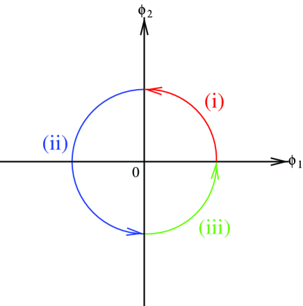
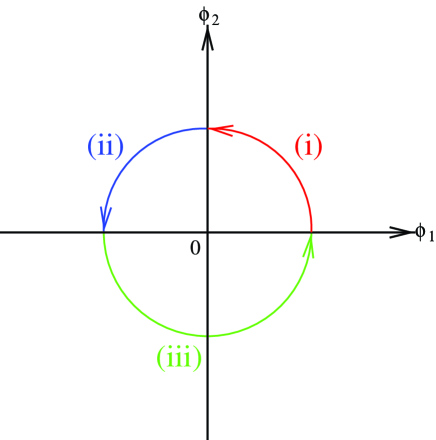
Figure 1: Left: Relative phase of the scalar fields is classified into three groups, (i) $0\leq\theta<\frac{\pi}{2}$, (ii) $\frac{\pi}{2}\leq\theta<\frac{3\pi}{2}$, (iii) $\frac{3\pi}{2}\leq\theta<2\pi$.
Right: Another classification of the relative phase, (i) $0\leq\theta<\frac{\pi}{2}$, (ii) $\frac{\pi}{2}\leq\theta<\pi$, (iii) $\pi\leq\theta<2\pi$, was also tried but the numerical results did not depend on these choices.

Figure 2: $\mbox{\boldmath${p}$}_{a}$ and $\mbox{\boldmath${q}$}_{a}$ are points corresponding to $\phi_{a}=0$ for each $a$. These points are obtained by linear interpolation using the values of $\phi_{a}$ at two corners of the plaquette between which it changes sign. The line $\phi_{a}=0$ for each $a$ is drawn by simply connecting $\mbox{\boldmath${p}$}_{a}$ and $\mbox{\boldmath${q}$}_{a}$ by a straight line. The intersection of these two lines is identified as the position through which a string penetrates a plaquette.

Figure 3: When the intersection is found outside the plaquette, the nearest point on the edge of the plaquette is identified as the penetration point of the string.

References

- (1)
- (2) T. W. B. Kibble, J. Phys. A 9, 1387 (1976).
- (3) L. A. Kofman and A. D. Linde, Nucl. Phys. B282, 555 (1987); Q. Shafi and A. Vilenkin, Phys. Rev. D 29, 1870 (1984); E. T. Vishniac, K. A. Olive, and D. Seckel, Nucl. Phys. B289, 717 (1987); J. Yokoyama, Phys. Lett. B 212, 273 (1988); Phys. Rev. Lett. 63, 712 (1989).
- (4) For a review, see A. Vilenkin and E. P. S. Shellard, Cosmic String and Other Topological Defects (Cambridge University Press, Cambridge, England, 1994).
- (5) V. M. H. Ruutu et al., Nature (London) 382, 334 (1996); Phys. Rev. Lett. 80, 1465 (1998); C. Baüerle et al., Nature (London) 382, 332 (1996).
- (6) P. C. Hendrey et al., Nature (London) 368, 315 (1994); M. E. Dodd et al., Phys. Rev. Lett. 81, 3703 (1998).
- (7) W. H. Zurek, Nature (London) 317, 505 (1985); for a review, W. H. Zurek, Phys. Rep. 276, 177 (1996).
- (8) T. W. B. Kibble, Nucl. Phys. B252, 227 (1985).
- (9) Y. Nambu, in Proceedings of International Conference on Symmetries & Quark Models Lectures at the Copenhagen Summary Symposium, 1970; T. Goto, Prog. Theor. Phys. 46, 1560 (1971).
- (10) A. Albrecht and N. Turok, Phys. Rev. Lett. 54, 1868 (1985).
- (11) A. Albrecht and N. Turok, Phys. Rev. D 40, 973 (1989).
- (12) D. P. Bennett and F. R. Bouchet, Phys. Rev. Lett. 60, 257 (1988); 63, 2776 (1989); Phys. Rev. D 41, 2408 (1990).
- (13) B. Allen and E. P. S. Shellard, Phys. Rev. Lett. 64, 119 (1990).
- (14) P. de Bernardis et al. Nature (London) 404, 955 (2000); R. Stompor et al. Astrophys. J. Lett. 561, L7 (2001); J. L. Sievers et al. astro-ph/0205387.
- (15) F. R. Bouchet, P. Peter, A. Riazuelo, and M. Sakellariadou, Phys. Rev. D 65, 021301 (2002); C. R. Contaldi, astro-ph/0005115.
- (16) G. R. Vincent, M. Hindmarsh, and M. Sakellariadou, Phys. Rev. D 56, 637 (1997); G. R. Vincent, N. D. Antunes, and M. Hindmarsh, Phys. Rev. Lett. 80, 2277 (1998).
- (17) R. D. Peccei and H. R. Quinn, Phys. Rev. Lett. 38, 1440 (1977).
- (18) A. Vilenkin and A. E. Everett, Phys. Rev. Lett. 48, 1867 (1982).
- (19) R. L. Davis, Phys. Rev. D 32, 3172 (1985); Phys. Lett. B 180, 225 (1986).
- (20) M. Kalb and P. Ramond, Phys. Rev. D 9, 2273 (1974); F. Lund and T. Regge, ibid. 14, 1524 (1976); E. Witten, Phys. Lett. 153B, 243 (1985).
- (21) M. Barriola and A. Vilenkin, Phys. Rev. Lett. 63, 341 (1989); D. P. Bennett and S. H. Rhie, ibid. 65, 1709 (1990); U. Pen, D. N. Spergel, and N. Turok, Phys. Rev. D 49, 692 (1994).
- (22) M. Yamaguchi, Phys. Rev. D 64, 081301(R) (2001); 65, 063518 (2002).
- (23) J. Preskill, Phys. Rev. Lett. 43, 1365 (1979).
- (24) J. Ye and R. Brandenberger, Mod. Phys. Lett. A 5, 157 (1990); Nucl. Phys. B346, 149 (1990).
- (25) M. Yamaguchi, J. Yokoyama, M. Kawasaki, Prog. Theor. Phys. 100, 535 (1998).
- (26) R. L. Davis and E. P. S. Shellard, Nucl. Phys. B324, 167 (1989); A. Dabholkar and J. M. Quashnock, ibid. B333, 815 (1990).
- (27) R. A. Battye and E. P. S. Shellard, Nucl. Phys. B423, 260 (1994); Phys. Rev. Lett. 75, 4354 (1995); Phys. Rev. D 53, 1811 (1996).
- (28) M. Yamaguchi, M. Kawasaki, and J. Yokoyama, Phys. Rev. Lett. 82, 4578 (1999).
- (29) M. Yamaguchi, Phys. Rev. D 60, 103511 (1999); M. Yamaguchi, J. Yokoyama, and M. Kawasaki, ibid. 61, 061301(R) (2000).
- (30) C. J. A. P. Martins and E. P. S. Shellard, Phys. Rev. D 65, 043514 (2002).
- (31) J. N. Moore, E. P. S. Shellard, and C. J. A. P. Martins, Phys. Rev. D 65, 023503 (2001).
- (32) D. Austin, E. J. Copeland, and T. W. B. Kibble, Phys. Rev. D 48, 5594 (1993); E. Copeland, T. W. B. Kibble, and D. Austin, ibid. 45, 1000 (1992).
- (33) C. J. A. P. Martins and E. P. S. Shellard, Phys. Rev. D 53, 575(R) (1996); 54, 2535 (1996).
- (34) M. Yamaguchi and J. Yokoyama, Phys. Rev. D 66, 121303(R) (2002).
- (35) T. Vachaspati and A. Vilenkin, Phys. Rev. D 30, 2036 (1984).
- (36) M. Hindmarsh, hep-ph/0207267.