Taming Asymptotic Strength

Abstract

Using a simple Asymptotically Strong N=1 Susy SU(2) Gauge theory coupled to a 5-plet Chiral superfield we demonstrate the plausibility of the “ truly minimal ” Asymptotically Strong Grand Unification scenario proposed by us recently. Assuming a dynamical superpotential consistent with the symmetries and anomalies is actually induced non-perturbatively we show the gauge symmetry is dynamically and spontaneously broken at a UV scale that is generically exponentially larger than the scales characteristic of the effective low energy theory. The pattern of condensates in a semi-realistic $SU(5)$ ASGUT is analyzed using the Konishi anomaly assuming condensation occurs as shown by our toy model. The necessarily complementary relation of ASGUTs to the Dual Unification program and the novel cosmogony implied by their unusual thermodynamic properties are also discussed.

I Introduction

In a recent feuilleton [1] we agitated for serious consideration of the possibility that the Grand Unification Gauge group becomes strongly coupled above the scale of perturbative unification ($M_{U}$). This behaviour is inevitable in any GUT containing Higgs fields capable of giving realistic fermion mass relations (FM Higgs) at tree level [2, 3] since the Casimir indices of such representations are generically large and hence drive the gauge coupling into the strongly coupled regime above their mass thresholds (the problem is especially acute in SO(10) Susy GUTs that employ 126-plets but the behaviour is generic ). We argued that the almost superstitious avoidance of Asymptotically Strong (AS) models in the literature was unjustified. The intuitive picture that emerges when the basic reversal of roles between the perturbative gauge non-singlet and the confined gauge singlet phases is accounted for, is quite appealing and does not violate any canon. Rather it raises the possibility of quite novel solutions and insights into the hoary puzzles of unification physics. Even if unrealized in nature it would constitute a remarkable logical completion that needs no banishment to the realm of the unthinkable.

Reversing the usual logic that sees fermion masses as a peripheral or second order issue relative to the primary fact of symmetry breaking we argued that their necessity in an important component of the inner rationale for symmetry breaking in the Standard Model (SM) and GUTs. The SM ensures an observable electromagnetic U(1) gauge symmetry only by ensuring that all charged particles are in fact massive. If this were not so then the massless charged particles would completely screen the U(1) charge at low energies thus rendering it unobservable. Moreover there are other pathologies associated with massless charged particles (of any spin) in both Quantum and Classical dynamics and this makes it all the more plausible that ensuring their absence in the SM via the formation the Higgs Condensate is a rationale behind the formation of the Higgs Condensate itself . The SM fermion mass spectrum is thus an important clue for the choice of Higgs representations and so to the mode of symmetry breaking of the GUT in which the SM is embedded. In a truly minimal (TM) model the low energy fermion mass and gauge coupling data and the Fermion Mass (FM) Higgs representations needed to fit it should determine the pattern and modality of unification completely. In our proposal it is the low energy data itself that forces us to take seriously the possibility of strong gauge couplings above the GUT scale. Else we must abandon painstakingly developed and otherwise sensible (Susy) GUTs e.g [7] where the presence of $\bf{126+{\overline{126}}}$ is used to implement see-saw mechanisms for neutrino mass in an SO(10) Susy GUT while preserving R-parity to low energies. The Casimir index of these two Higgs multiplets alone is thrice that of the gauge fields !

Furthermore, the presence of effectively exact Supersymmetry at the GUT scale ($\Lambda_{U}>>M_{S}$) fairly cries out for exploitation, given all the attendant simplifications. This is in sharp contrast to the case of “realistic” SQCD where the supersymmetry breaking scale completely dominates the condensation scale ($M_{S}>>\Lambda_{QCD}$) and relegates the conclusions derived from Susy QCD largely to the realm of the qualitative [8] and the inapplicable. As we have shown elsewhere [4, 5, 6, 7] Susy makes the analysis of symmetry breaking patterns and phenomenology tractable even in very complex models. The enhanced analyzability is conferred by the special holomorphicity and non renormalization properties of Supersymmetric theories [9, 11, 10, 12]. Thus N=1 strongly coupled Susy GUTs are prime candidates for application of the techniques developed for the analysis of phase portraits of Susy Gauge theories [9, 10, 12, 13, 14]. Unfortunately, Asymptotically Strong (AS) models have received at most passing mention in the enormous literature devoted to the dynamics of Susy gauge theories. From time to time, the possibility of AS Unified theories (albeit with considerably larger gauge groups than standard GUTs) has been resurrected [16] but no particular merit of uniqueness or genericity has been available to justify the extensions proposed . Moreover it was unclear how any significant step beyond the bald statement of UV strength could be made about the UV dynamics of such theories and its relevance to the structure of the low energy theory.

In [1] we proposed that the (scale inverted) analogy of AS theories with familiar strong coupling QCD dynamics suggests a very appealing intuitive picture of the effect of AS. Since the low energy and long distance theory is weakly coupled the principal effects of the strong coupling in the UV are likely to be in the formation of condensates that break gauge symmetry and thus define the vacuum of the perturbative effective gauge theory at larger length scales $>>\Lambda_{U}^{-1}$. Such condensates would also directly modify our picture of the nature of elementary particles at the smallest scales where the gauge flux would be strongly self attracting. This picture also suggested a close connection with Dual unification [17] in which matter elementary particles are seen as monopole solitons of a dual gauge theory. Indeed the dual unification picture becomes much more coherent, consistent and plausible when seen as the dual of an AS Susy GUT; as indeed is required by its very assumptions.

For these reasons we think it necessary and possible to investigate the scenario in which FM Higgs residuals with mass thresholds just above the scale of perturbative unification ($M_{U}$) drive the gauge coupling into the strong coupling regime at a scale $\Lambda_{U}$ which is quite close to $M_{U}$ in realistic models. The energy ranges that need to be characterized divide naturally into three : I)  the UV strong coupled regime ($E>\Lambda_{U}$) II) the perturbatively coupled supersymmetric intermediate regime $\Lambda_{U}>E>M_{S}$ and III) the standard low energy MSSM/SM regime below the supersymmetry breaking scale : $M_{S}>E$. We shall take the pragmatic epistemic position that the theoretical task is no more than to construct economical and minimal models within which each of these qualitatively distinct regimes can be quantitatively characterized and their dynamics understood via simple “pictures” of the processes involved. The relation and translation between the effective theories that characterize each regime, and their derivation from the underlying fundamental gauge theory, is $-$ as familiar from QCD and Chiral Perturbation theory $-$ expectedly a difficult problem that we may expect to resolve only semi-quantitatively in an analytic context.

We argue that the novel interpretative context of UV condensation (regime I) and GUT scale to QCD scale liberation of gauge variant degrees of freedom(regime II) makes available new - and pleasing - possibilities that can further our insight into the nature of elementarity and unification. For clarity and definiteness we choose a simple renormalizable AS model consisting of N=1 Susy SU(2) Gauge theory coupled to a Chiral multiplet transforming as a 5 dimensional SU(2) irrep and ask what are the effective theories that characterize its behaviour in the regimes described above. We make the plausible assumption that in the crucial intermediate energy perturbative regime II the relevant degrees of freedom are the usual gauge non-singlet ones described by the N=1 Susy YM lagrangian with a renormalizable tree level superpotential $W_{t}$ and a dynamically induced superpotential arising from non-perturbative dynamics in a manner consistent with holomorphicity, anomalies and global (super)symmetries in complete analogy with the well established dynamical superpotentials that arise in the AF case [9, 10, 12, 13, 14]. In region I we take the relevant degrees of freedom to be (‘t Hooft anomaly matched ) gauge singlet chiral moduli interacting via the same dynamical superpotential as in the perturbative regime but differing in (at least) an independent and unknown Kahler potential. We assume that the deviations from the canonical form of the Kahler potential (and the gauge kinetic chiral functions) in the perturbative region II are negligible (see Section II). This ansatz is in accord with the standard picture of confinement enforced on non-gauge particles by singular wave function renormalization, and, correspondingly, the divergence of their renormalized effective masses. In the perturbative region II we can extract significant information using the definition of the moduli as polynomial composites in the chiral multiplets. Region III or the Susy EW breaking/QCD confining regime is governed by the standard MSSM/SM dynamics.

The plan of the paper is as follows. In Section II we set out our scenario and intuitive picture of how an AS GUT works. In Section III we define and discuss the strongly coupled SU(2) Gauge plus quintet Higgs model referred to above and obtain the possible vevs of the Higgs fields . In Section IV we discuss the pattern of dynamical symmetry breaking (DSB) and gaugino condensation implied by the vevs of Section III and the constraints on the dynamical superpotential that may be inferred using the Konishi Anomaly[15] and decoupling arguments. In Section V we discuss the lessons and implications of our simple model for the project of constructing viable realistic AS GUTs. We conclude in Section VI with a discussion of the appealing relation ASGUTs necessarily and naturally enjoy with the Dual unification picture [17] in which the elementary particles of the SM appear as monopoles of a dual gauge group and how it resolves otherwise problematic features of those models. We thus motivate a new, supersymmetric, version of the dual unification scenario[41]. Finally we discuss the ASGUT novel cosmogony implied by liberation of degrees of freedom by cooling in ASGUT thermodynamics.

II AS Dynamical Scenario

A plausible picture of the dynamics of AS theories may be drawn using the analogy with the known features of IR strong gauge theories. The reversal of the roles of small and large length scales in the case of AS theories turns the usual picture of confinement “inside out”. It is this conceptual leap , diametrically opposed yet closely analogous to the inbred picture of QCD and its effective low energy theory of colour singlet hadrons that jumps the barrier to realizing that AS theories can be an equally consistent “other half” of the space of Yang Mills theories.

When the gauge coupling becomes strong one expects gauge singlet condensates (in particular the gaugino condensate familiar from Susy QCD) to form and to be characterized by a scale $\Lambda_{U}$ ($\equiv\Lambda$) at which the (one-loop) RG equations indicate a divergence in the gauge coupling . Above $\Lambda$ the gauge non-singlet degrees of freedom become confined due to singular wavefunction renormalizations which give them infinite effective masses. Thus the residual dynamics must involve suitable gauge singlet degrees of freedom. It is natural to choose the D-flat moduli which are so central in Asymptotically Free (AF) Susy theories for the leading role in the AS UV dynamics as well since their masses are less than the typical energies in region I. As in the AF case the ’t Hooft anomaly matching conditions[18] serve as a valuable cross check of the completeness and consistency of the set of modes retained.

The electric permeability of the UV condensates must exhibit the peculiar inversion referred to above : self attraction of a point particle’s electric flux (equivalently strong screening by the condensate) implies that it should form a gauge singlet tangle or ball of size $\sim\Lambda^{-1}$ surrounding the putative point charge. This tangle will not be resolvable by any gauge non singlet probe: thus conferring an elementary size on fundamental gauge non-singlet particles. On larger scales however the electric flux is weakly coupled and hence the gauge charge of an elementary particle will appear as the source of flux streaming out freely (on scales $>>l=\Lambda^{-1}$) from a gauge singlet core (see Fig.1) characterized by the gauge charge as a “surface ” parameter (somewhat like the quantum numbers of a black hole in the horizon-membrane picture [21]). Such a structure could be described as a soliton or bag of the Chiral gauge singlet dynamics used to characterize the high energy phase of the theory married to the perturbative gauge theory at the core boundary .

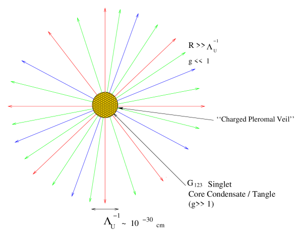
FIG. 1.: The Pleromal Heart of a Quark : The interior of the core condensate cannot be probed by charged probes and the quark charge is a surface parameter of the core tangle.

Since the gauge coupling is small below $M_{U}$ the low energy dynamics is a perturbative theory of gauge non-singlet particles interacting with the massless gauge bosons of the gauge symmetry left unbroken by the condensation at the UV scales. This is in sharp contrast to QCD where the perturbative dynamics is indifferent to the confining condensates precisely because the energy scales of the perturbative theory are much larger than those of the QCD condensates ($\Lambda_{QCD}$ functions as an IR cutoff). Our prescription for unravelling the very novel features presented by AS UV condensation is thus to replace the fundamental Gauge theory by effective field theories in each of the dynamical regions. For region I ( energy scales $E>\Lambda_{U}$) we propose a theory of the anomaly matched gauge singlet Chiral moduli ($X_{(n)}$) of the fundamental N=1 Susy Gauge model interacting according to a dynamical superpotential $W_{d}(X_{(n)},\Lambda,m,\lambda)$ (in addition there is the tree superpotential of the fundamental theory which depends on the masses and couplings $m_{i},\lambda_{i}^{(n)}$ of the Chiral multiplets $\Phi_{(i)}$) which represents the strong coupling dynamics. The Kahler potential in region I $K_{I}(X,X^{*})$ is a highly non perturbative object representing the condensation of the moduli theory and the confinement of the gauge and gauge variant chiral modes. However one could still apply supersymmetric chiral perturbation theory techniques to it in direct analogy with the AF case [8]. Many of the features of $W_{d}$ can be deduced or constrained on the basis of (super)symmetry, holomorphicity and decoupling requirements [13]. In the perturbative regime II, $\Lambda_{U}>E>M_{S}$, we have the effective spontaneously broken gauge theory of modes left light by the UV condensation of the gauge singlet moduli. Such a theory will be described by three functions : the Kahler potential $K_{II}(\Phi,\Phi^{*})$, the superpotential $W(\Phi)=W_{d}+W_{t}$ and the chiral gauge kinetic coupling function $f^{ab}_{II}(\Phi)$. In this paper we shall focus on Region II and the effects coded in the superpotential $W_{d}$ assuming the Kahler potential and gauge kinetic function are effectively canonical. Note however that while a canonical Kahler potential for the perturbative modes is a reasonable assumption , the effects of a non-canonical gauge kinetic function can be critical for issues of supersymmetry breaking in the presence of gravity [19]. Indeed it is very interesting to study[41] the generation of non-canonical structure in this function in $N=2$ AS theories (or perturbations thereof) where one can seek to apply the techniques developed [20] for N=2 AF theories.

An important consistency check on the set of gauge singlet moduli retained in the UV effective theory of region I is that they should satisfy the ’t Hooft anomaly matching conditions [18, 13, 14] for the unbroken global symmetries of the model with respect to the anomalies calculated using the gauge non singlet or fundamental spectrum. In IR strong models this set is found to exclude the glueball chiral superfield $S=(1/32\pi^{2})W^{a}_{\alpha}W^{a\alpha}$ (where $W^{a}_{\alpha}$ is the (bare) chiral gauge supermultiplet in ‘holomorphic’ normalization[22, 23, 24]. We also find that the anomaly matching conditions exclude S from the singlet spectrum for region I. As in the IR strong case, S plays a vital role in understanding the strong coupling condensates since the Konishi anomaly [15] furnishes the value of the gluino condensate (i.e the scalar component of $S$) in terms of the expectation value of the chiral condensates . In the initial studies [9] low energy effective actions were built including this glueball field. Then one can code in the anomalies of the theory into the effective Lagrangian since the Glueball superfield $S$ contains $F^{a}_{\mu\nu}{\tilde{F}}_{a}^{\mu\nu}$ in its auxiliary component. However it was argued [12] that the effective low energy action can lead to misleading and ambiguous answers if only a partial set of the “heavy” degrees of freedom is included in it. This caveat is supported by the fact that inclusion of the glueball field S along with the singlet moduli in the effective theory typically violates the ’t Hooft anomaly matching conditions for the unbroken global symmetries. On the other hand it is not clear that inclusion of a finite set of additional composite fields could not cancel the contribution of the glueball field. Then this additional anomaly matched set, being qualitatively lighter than the coloured fields which have receded to infinite running mass, could play a useful role in describing the dynamics of modes with masses less than or near to the confinement scale or even of massless modes that could appear as bound states . In any case the action with $S$ can serve the useful functions described above even if it is not trustworthy for quantitative dynamics.

The Konishi Anomaly relations[15] are superfield $U(1)_{c}$ Ward-Takahashi identities that arise when the non-invariance of the path-integral measure under an arbitrary chiral superfield rephasing of individual chiral superfields $\Phi_{(i)}$ is taken into account. In the absence of sources it reads ($V_{i}$ is the gauge vector superfield)

$$0=\Big{\langle}-{{\bar{D}}^{2}\over 4}{\bar{\Phi}^{(i)}}exp[V_{i}]\Phi_{(i)}+\Phi_{(i)}{{\partial W_{tree}}\over{\partial\Phi_{(i)}}}+{{2T_{(i)}}\over{32\pi^{2}}}W^{a\alpha}W^{a}_{\alpha}\Big{\rangle}$$ (1)

The lowest component of the Konishi anomaly yields a very useful set of relations involving the gaugino condensate $\langle S|_{\theta=0}\rangle=\langle(-\lambda^{a}\lambda^{a}/32\pi^{2})\rangle$ and vevs of the different invariants formed from chiral superfield scalar components corresponding to the chiral invariants occurring in the tree superpotential $W_{tree}$:

$$\langle S\rangle=-{1\over{2T_{(i)}}}\Big{\langle}\phi_{(i)}{{\partial W_{tree}}\over{\partial\phi_{(i)}}}+{1\over{2\sqrt{2}}}\{{\bar{Q}}_{\dot{\alpha}},{\bar{\psi}}^{\dot{\alpha}i}\phi_{i}\}\Big{\rangle}$$ (2)

There is no sum over the index $(i)$, $T_{(i)}$ is the index of $(i)$th representation in the normalization where the fundamental is $1/2$, and $W_{tree}$ is the tree level superpotential of the underlying gauge theory. The vev of the anticommutator with the supercharge ${\bar{Q}}_{\dot{\alpha}}$ above vanishes to the accuracy that supersymmetry is preserved. On dimensional grounds its value can be tentatively estimated as $M_{S}^{3}$ or perhaps as $\sim M_{S}^{2}\langle\phi_{i}\rangle$. A clearer understanding of its role can come about only once the source of supersymmetry breaking in the theory is specified (see Section 6) and the effect of soft supersymmetry breaking terms on the derivation of the Konishi Identities eqn.(1) determined. In eqn.(2), in the limit of exact supersymmetry, the glueball field S is not renormalized perturbatively and nor is $W_{tree}$ or the operators $\Phi_{(i)}\partial/\partial\Phi_{(i)}$. Thus we may expect that this relation is RG invariant and should be respected at all scales to the accuracy to which supersymmetry is preserved. On the other hand, since a realistic model will have soft Susy breaking masses that violate Susy explicitly in the Lagrangian , the assumptions of the derivation of eqns(1,2) will not hold and thus, at least till we have better control on the mechanisms of Susy breaking in ASGUTs, we should not trust these relations to an accuracy better than $M_{S}^{3}$ or perhaps $M_{S}^{2}\langle\phi\rangle$ .

These equations thus impose strong restrictions and requirements on the pattern of condensates in the theory. In the presence of a tree superpotential we expect that gaugino condensation at a scale $\Lambda$ implies UV condensation of moduli (and relations among different moduli vevs) and vice versa at least as long as supersymmetry is unbroken. In the perturbative theory the moduli are defined as polynomials in the gauge variant chiral fields and their (large) vevs determine the broken symmetry of the low energy gauge theory while characterizing it in a gauge invariant way. A subtle but inescapable possibility in this regard is that of quantum phase transitions in which e.g the product of two Higgs fields obtains an expectation value but not the fields themselves. This is a real possibility since the scale of perturbative unification $M_{U}$ is sufficiently close to the UV strong coupling scale $\Lambda_{U}$ to make quantum condensates important. However we shall resist the temptation of invoking such condensates, until and unless it is unavoidable, so as to retain maximal calculability in the effective gauge theory below the GUT scale. The effective low energy field theory must thus be shown to be compatible with the these very novel quantum vevs of gauge singlet composite operators which preserve all the symmetries of the theory, by definition.

III SU(2) AS model

Our model consists of a N=1 Susy SU(2) Gauge theory coupled to a SU(2) 5-plet ($SU(2)$ spin $j=2$) Chiral superfield presented as a symmetric traceless $3\times 3$ matrix: $\Phi_{ij}=\Phi_{ji};\Phi_{ii}=0;i,j=1,2,3$ . The additional feature relative to the familiar adjoint representation is that such a complex symmetric matrix cannot, in general, be diagonalized by a complex orthogonal transformation. However one observes that firstly the (upper triangular) Jordan canonical form of $\Phi$ is

$$\Phi=S\left(\begin{array}[]{ccc}a&c&d\\ 0&b&e\\ 0&0&-(a+b)\end{array}\right)S^{-1}$$ (3)

so that $X_{(n)}=Tr\Phi^{n}=a^{n}+b^{n}+(-(a+b))^{n}$ are dependent on only two independent complex numbers $a,b$ and as such only two of them, say the quadratic and cubic invariants $X_{(2)}=X,X_{(3)}=Y$, need be considered independent.

This can also be seen from the less familiar result that complex orthogonal transformation by $O_{c}$ can be used to put [25] a complex symmetric matrix in a block diagonal canonical form :

$$\Phi=O_{c}Diag(B_{1},B_{2},.....)O_{c}^{T}$$ (4)

where a diagonal block $B_{i}$ is either a $1\times 1$ submatrix consisting of an eigenvalue of $\Phi$ or a $q\times q$ symmetric submatrix of form $\lambda_{i}I+E_{i}$ where $\lambda_{i}$ is an eigenvalue and $E_{i}$ has all its eigenvalues zero, all its eigenvectors quasi-null and an eigenspace of dimension $d\leq q$. The matrices $E_{i}$ arise because in general a complex symmetric matrix can have invariant eigen-subspaces of zero Euclidean length. However in the present instance the additional freedom associated with these subspaces is irrelevant to definition of the gauge singlet moduli and also to the extremization of the superpotential w.r.t the field $\Phi$. The D-terms can be written as a commutator $[\Phi,\Phi^{\dagger}]$ . After fixing the $SU(2)_{c}$ gauge freedom by putting $\Phi$ in the canonical form (4) one sees that the pseudo-moduli contained in $E_{i}$ must vanish so that one can work with the diagonal form .

The index of the 5-plet (in the normalization where the fundamental has index $1/2$) is $10$ . Thus this theory has a one loop gauge beta function $\beta(g)=-b_{0}g^{3}/16\pi^{2};b_{0}=3\times 2-10=-4$ and hence its coupling grows in the ultraviolet. In the absence of a superpotential the underlying theory has $U(1)_{\Phi}$ symmetry under which the chiral superfield $\Phi$ has charge 1 and in addition a $U(1)_{R}$ R-symmetry under which the Grassman coordinate $\theta_{\alpha}$ has charge 1 , the gaugino -1 and the components $(A,\psi,F)$ of $\Phi$ have charges (0,1,2) respectively. Both these symmetries have mixed $U(1)SU(2)^{2}$ anomalies but the linear combination

$${\widehat{Q}}={1\over 2}(\sum_{i}T(i)(q^{0}_{i}Q_{\Phi}-q_{i}^{\Phi}Q_{0}))=4Q_{\Phi}-5Q_{0}$$ (5)

generates a non anomalous U(1) R symmetry. The charges of the various Chiral superfields and components (and of the holomorphic parameters introduced below) are given in Table I.

Field	$Q_{\Phi}$	$Q_{0}$	${\widehat{Q}}$
$\theta_{\alpha}$	0	1	-5
$\Phi$	1	0	4
$\psi_{\Phi}$	1	1	-1
$\lambda_{\alpha}$	0	-1	5
$S$	0	-2	10
$m$	-2	-2	2
$\lambda$	-3	-2	-2
$\Lambda^{-4}$	20	16	0
$\Lambda_{d}^{3}$	0	-2	10

Table 1 :$\quad U(1)$ charges of fields and parameters.

The contributions of the elementary fermions to the ${\widehat{U(1)}}^{3}$ and ${\widehat{U(1)}}$ (gravitational) anomalies are $370=3\cdot 5^{3}+5\cdot(-1)^{3}$ and $3\cdot 5+5\cdot(-1)=10$ respectively . The fermionic components of the moduli fields i.e $\psi_{X,Y}$ have ${\widehat{U(1)}}$ charges 3,7 and hence precisely match these anomalies . The glueball field $S=(32\pi^{2})^{-1}W^{a}_{\alpha}W^{a}_{\alpha}$ cannot therefore be consistently included alone in the relevant degrees of freedom.

The most general renormalizable tree superpotential is

$$W_{t}=-{m\over 2}X+{\lambda\over 3}Y$$ (6)

Prima facie this potential violates all the $U(1)$ symmetries . However by considering[12] the parameters $m,\lambda$ as expectation values of chiral fields one can exploit the holomorphicity of the Susy theories w.r.t chiral fields and hence we assign the charges shown in Table I to $m$ and $\lambda$ so as to formally preserve the $U(1)$ symmetries.

The one loop gauge coupling evolution in the range $\Lambda_{U}>\mu>m$ is

$${1\over{g^{2}(\mu)}}={1\over{g^{2}(m)}}-{4\over{8\pi^{2}}}ln{\mu\over m}$$ (7)

If the Higgs field decouples completely and leaves an unbroken pure $SU(2)$ gauge theory below the scale $m$ the in the range $m>\mu>\Lambda_{d}$ the gauge coupling evolves as

$${1\over{g^{2}(\mu)}}={1\over{g^{2}(m)}}+{6\over{8\pi^{2}}}ln{\mu\over m}$$ (8)

Here $\Lambda_{U}$ is the scale where the (one-loop) running coupling of the AS model diverges (henceforth abbreviated to $\Lambda$) and $\Lambda_{d}$ the corresponding scale for the effective theory in which the Higgs multiplet has decoupled completely without breaking the symmetry. It can also happen that the Higgs multiplet breaks the symmetry partially : i.e in this case down to U(1). In that case the low energy theory will be a pure $U(1)$ gauge theory coupled to charged Higgs remnants (if any) and the $U(1)$ gauge coupling evolves accordingly and must be matched at the scale $m$ to the coupling in the high energy theory. However, in more complicated models with larger gauge groups, the low energy symmetry can be non-abelian. Let $m_{t}$ be a notional low energy scale where the gauge coupling of the low energy effective theory is specified , then by matching gauge couplings of the UV and IR theories at the threshold $m$ (in the DR scheme)[9, 10, 13, 27] one gets

$$\Lambda_{d} = m_{t}e^{({-{4\pi^{2}}\over{3g^{2}(m_{t})}})}=me^{({-{4\pi^{2}}\over{3g^{2}(m)}})}$$ (9)

$$\Lambda = me^{({2\pi^{2}\over{g^{2}(m)}})}=({{m^{5}}\over\Lambda_{d}^{3}})^{1\over 2}$$ (10)

$$\epsilon = {m\over\Lambda}=({{\Lambda_{d}}\over m})^{3\over 2}=({{\Lambda_{d}}\over{\Lambda}})^{3\over 5}$$ (11)

It is important to note that the decoupling parameter $\epsilon$ must be taken to zero as $m,\Lambda\rightarrow\infty$ while keeping $\Lambda_{d}$ constant for consistency.

When building effective superpotentials invariant under all symmetries (anomalous or not) it is also useful to assign $\Lambda^{b_{0}}$ the charges 20,16,0 and use $\Lambda$ to adjust dimensions in dynamical expressions[13, 14]. Proceeding in the familiar way [13] one finds that the symmetries of the theory restrict the dynamical superpotential to the form

$$W_{d} = X^{5\over 4}\Lambda^{1\over 2}{\widehat{W}(v,w,z)}+\Lambda_{d}^{3}f({{m\lambda}\over\Lambda})$$ (12)

$$v = X^{3}/6Y^{2}\qquad w=m/X^{1\over 4}\Lambda^{1\over 2}\qquad z=\lambda X^{1\over 4}/\Lambda^{1\over 2}$$ (13)

Note that the exponent of $\Lambda$ ($T=10$ is the index of the Higgs, N=2 the gauge Casimir) is $(3N-T)/(N-T)$ and thus has the form familiar from QCD but is positive due to a double negative (numerator and denominator). As is well known, these exponents are determined by symmetry and dimensional analysis coupled with the renormalization group [9, 11, 13]. The unknown function $\widehat{W}$ is a power series

$${\widehat{W}}=\sum_{\alpha,\beta}{\widehat{W}}_{\alpha,\beta}(v)w^{\alpha}z^{\beta}=\sum{\widehat{W}}_{\alpha,\beta}(v)m^{\alpha}\lambda^{\beta}\Lambda^{-{{(\alpha+\beta)}\over 2}}X^{{\beta-\alpha}\over 4}$$ (14)

As in the case of QCD such a function can, presumably, arise via (fractional) instanton or other non-perturbative effects. Our basic assumption and approximation is that $W_{d}$ is non zero and admits an expansion in the perturbing parameters $m,\lambda$. As we shall see, the presence of such a function, which respects all symmetries and anomalies, allows one to implement the demands of decoupling in a straightforward manner and presents no difficulties of the sort one might expect to encounter if it was forbidden for deep reasons. On the contrary, we show that the consistency of the physical picture requires a dynamical superpotential, or at least a constraint implementing condensation. It is perhaps worth noting that even in the well studied case of Susy QCD the amplitude of the induced superpotential is only reliably calculable[27, 28], so far, in the case $N_{f}=N_{c}-1$ while the amplitudes in all cases where fractional powers of $\Lambda^{b_{0}}$ enter are deduced only on the basis of decoupling. Note that if the function $\widehat{W}$ respects the form of the (fractional) instanton expansion then (schematically)

$$W_{d}\sim(\sum_{n=1}\Lambda^{nb_{0}})^{{1\over{(N-T)}}}\sim\Lambda^{b_{0}\over{N-T}}(1+{1\over{N-T}}\Lambda^{b_{0}}+....)\sim\Lambda^{1\over 2}(1+\Lambda^{-4}+..)$$ (15)

Where we have written the instanton suppression factor $e^{-8\pi^{2}/g^{2}}$ as $\Lambda^{b_{0}}$ using the one loop definition of $\Lambda$. Thus in eqn.(14) $\alpha+\beta=8n,n=0,1,2...$. Since we regard the superpotential parameters as small perturbations to the main dynamics we see that to leading order in $m,\lambda$ we can write

$$W={\Lambda^{3}}[x^{5\over 4}G(v)-{\epsilon\over 2}x+{\lambda\over 3}y]$$ (16)

where $x=X/\Lambda^{2},y=Y/\Lambda^{3},\epsilon=m/\Lambda=(\Lambda_{d}/m)^{3/2}$ are dimensionless and we have dropped the constant term as irrelevant. Our assumption is thus that, at least in the perturbative regime, the superpotential $W_{d}$ represents the main non-perturbative effects. Its implications for the vacuum structure can be evaluated by extremizing it w.r.t the perturbative field $\Phi$. The same result may also be obtained by demanding [9] that a superpotential dependent on $X,Y$ and the glueball field $S$ reproduce the ABJ anomalies and be invariant under the $\widehat{U(1)}$ symmetry. In that case one finds that

$$W_{d}(X,Y,S)=S[ln{{X^{10}\Lambda^{4}H(v,{{mX}\over S},{{\lambda X^{3\over 2}}\over S})}}]-8SlnS$$ (17)

satisfies all the conditions imposed even if $H$ is taken to be an arbitrary power series in its arguments. From such a superpotential one could, given H, eliminate $X,Y$ using the vacuum equations of motion , to obtain a superpotential $W(S,m,\lambda)$ which can be used to characterize the gaugino condensate in the vacuum of the low energy pure gauge theory. In the process one finds, to leading order in $m,\lambda$ the Konishi anomaly relation eqn(2). Conversely, in the same approximation, if one eliminates the field $S$ in favour of $X,Y$ one finds $W_{d}=8\langle S\rangle(X,Y)$. The Konishi relation eqn.(2) between gaugino ($S$) and chiral multiplet ($X,Y$) condensates is then readily seen to follow from from the extremization of the total superpotential. The effects of the $m,\lambda$ dependence of $H$ appear as corrections. Recently remarkable claims have appeared [29] regarding the calculability of the full ($m,\lambda$) corrections to $W(S)$ and $\langle W\rangle(m,\lambda)$ via large $N_{c}$ matrix models (at least in theories where the chiral multiplets can be written as matrix representations of the gauge group). Such results would permit evaluation of the chiral condensates and (via a Legendre transform) construction of $W_{d}$ . Moreover the Konishi relation eqn(2) is a rigorous relation that should be obeyed to all orders in the parameters $m,\lambda$ and this will also constrain $H$. Since we are here working only to leading order in $m,\lambda$ the form of our superpotential is already consistent with the Konishi Anomaly relation as explained. One gets

$$\langle S|\rangle=-{1\over{20}}\sum_{A=1}^{5}\phi_{A}{\partial\over{\partial\phi_{A}}}W_{t}={1\over{20}}(mX|-\lambda Y|)$$ (18)

The $|$ refers to taking the scalar component and will be implicit hence forth. Since the limit $\Phi\rightarrow 0$ should be nonsingular for AS theories, the behaviour of the unknown dynamical function $G(v)$ as $v\rightarrow 0,\infty$ is constrained. If $\gamma_{0},\gamma_{\infty}$ are the exponents of G in these limits then one obviously has $\gamma_{0}\geq-{5\over{12}},\gamma_{\infty}\leq 0$ since these represent the conditions required to approach $X=0$ at constant $Y$, and $Y=0$ at constant $X$, respectively, without $W_{d}$ becoming singular. The vanishing of the $F_{\Phi}$ terms gives

$$2\Lambda{W}_{x}\Phi+3{W}_{y}(\Phi^{2}-{1\over 3}tr\Phi^{2})=0$$ (19)

where

$${W}_{x}=x^{1\over 4}({5\over 4}G(v)+3vG^{\prime}(v))-{\epsilon\over 2}$$ (20)

$${W}_{y}=x^{-{1\over 4}}(-2{\sqrt{6}}v^{3\over 2}G^{\prime}(v))+{\lambda\over 3}$$ (21)

The solutions to these equations can be divided into

A) Singlet mode solutions which arise when $W_{x}=W_{y}=0$ .

B) Perturbative mode solutions which arise when $W_{x},W_{y}$ are both non zero.

A) Singlet mode solutions

Multiplying the two equations in $W_{x}=W_{y}=0$ using eqns.(21) we get

$$({5\over 2}G(v)+6vG^{\prime}(v))(6v)^{3\over 2}G^{\prime}(v))={{\epsilon\lambda}}=\eta$$ (22)

thus given $G(v)$ one can determine $\langle v\rangle$, while the second of eqns(21) fixes $X$ once the value of $v$ is found :

$$\langle x\rangle^{1\over 4}=\langle{{(6v)^{3\over 2}G^{\prime}(v)}\over\lambda}\rangle$$ (23)

We now perturb in the small parameter $\eta$ . Three types of solutions can exist depending on the solution $v_{0}$ of the equation

$$(5G(v_{0})+12v_{0}G^{\prime}(v_{0}))(6v_{0})^{3\over 2}G^{\prime}(v_{0}))=0$$ (24)

These are

• $v_{0}$ non-zero and finite and determined by

$$5G(v_{0})+12v_{0}G^{\prime}(v_{0})\equiv 5G_{0}+12v_{0}G_{0}^{\prime}=0$$ (25)

• $v_{0}=0\qquad\qquad$ iii) $v_{0}=\infty$.

The exponents and amplitudes of perturbation in the small parameter $\eta$ are defined as :

$$\langle v\rangle =v_{0}+v_{1}\eta^{\delta}+.....$$ (26)

$$\langle x\rangle =x_{0}+x_{1}\eta^{\theta}+.......$$ (27)

$$\langle y\rangle =y_{0}+x_{1}\eta^{\omega}+.......$$ (28)

i) $v_{0}\neq 0,\infty$

When $v_{0},G_{0}^{\prime}$ are non zero one finds

$$x_{0} = (5{\sqrt{3v_{0}\over 2}}{G_{0}\over\lambda})^{4}$$ (29)

$$y_{0} = {{x_{0}^{3\over 2}}\over{\sqrt{6v_{0}}}}$$ (30)

Continuing one can find the higher order corrections . Thus $\delta=\theta=\eta=1$ and $v_{1},x_{1},y_{1}$ are determined in terms of $v_{0}$ and the derivatives of $G(v)$ at $v_{0}$. This type of solution generically gives

$$X\sim{\Lambda^{2}\over\lambda^{4}},\qquad Y\sim{\Lambda^{3}\over\lambda^{6}}\qquad i.e\qquad\Phi\sim{\Lambda\over{\lambda^{2}}}$$ (31)

and thus represents dynamical breaking of the gauge symmetry at the strong coupling scale $\Lambda$. The gauginos also condense strongly (see the next section for a discussion). Clearly in the absence of further information about $G(v)$ there is nothing useful further to say. In the other two cases the solutions are governed by the exponents $\gamma_{0,\infty}$ of the function $G(v)$ as $v\rightarrow 0,\infty$

b) $\quad v_{0}=0$

In this case the exponent $\delta$ must be positive for consistency . Provided $\gamma_{0}\neq 0,-5/12$ one finds

$$\delta = {2\over{4\gamma_{0}+1}}\Rightarrow\gamma_{0}>-{1\over 4}$$ (32)

$$\theta = {{4+8\gamma_{0}}\over{1+4\gamma_{0}}}$$ (33)

$$\omega = {{5+12\gamma_{0}}\over{1+4\gamma_{0}}}$$ (34)

and

$$v_{1}=({2\over{6^{3\over 2}\gamma_{0}h_{0}^{2}(5+12\gamma_{0})}})^{2\over{4\gamma_{0}+1}}$$ (35)

(36)

$$<x>^{1\over 4}=({2\eta^{{1+2\gamma_{0}}\over{1+4\gamma_{0}}}\over{h_{0}\lambda(5+12\gamma_{0}))v_{1}^{\gamma_{0}}}})+......$$ (37)

The requirement that $X,Y$ decouple as $m\rightarrow\infty$ amounts to requiring that $\theta>10/3$ and $\omega>5$ . Thus $X$ vanishes as $m\rightarrow\infty$ provided $-1/4<\gamma_{0}<1/8$ and $Y$ vanishes if $-1/4<\gamma_{0}<0$ i.e both decouple only if $-1/4<\gamma_{0}<0$ .

The values $\gamma_{0}=0,-{5\over{12}}$ are seen to be special from eqn.(37) and need separate treatment. In these cases the next to leading order exponents of G are important :

$$G(v)_{v\to\infty}\longrightarrow g_{0}v^{\gamma_{0}}+g_{0}^{\prime}v^{\gamma_{0}^{\prime}}+...$$ (38)

i) $\gamma_{0}=0$ , $\gamma_{0}^{\prime}>\gamma_{0}$, by definition, and one finds

$$\delta = {{2}\over{1+2\gamma_{0}^{\prime}}}\Rightarrow\gamma_{0}^{\prime}>-{1\over{2}}$$ (39)

$$\theta = 4$$ (40)

$$\omega = 6-{\delta\over 2}$$ (41)

Thus $X,Y$ both decouple as $m\rightarrow\infty$ and the decoupling connection to the pure $SU(2)$ gauge theory left behind fixes $g_{0}$ (see the next section).

ii) $v_{0}=-{5\over{12}}$ Now one finds

$$\delta = {{12}\over{1+12\gamma_{0}^{\prime}}}\Rightarrow\gamma_{0}^{\prime}>-{1\over{12}}$$ (42)

$$\theta = {4\over{1+12\gamma_{0}^{\prime}}}$$ (43)

$$\omega = 0$$ (44)

Although $X$ decouples for $1/60>\gamma_{0}^{\prime}$, $Y$ diverges as $m\rightarrow\infty$ so that symmetry is broken completely and strongly .

c) $v_{0}=\infty$

i) Here there is again the special case when the leading term in $G(v)$ is a constant:

$$G(v)\longrightarrow g_{\infty}+g_{\infty}^{\prime}v^{\gamma_{\infty}^{\prime}}$$ (45)

Since now $\delta<0$ for consistency one finds

$$\delta = {2\over{1+2\gamma_{\infty}^{\prime}}}\Rightarrow\gamma_{\infty}^{\prime}<-{1\over 2}$$ (46)

$$\theta = 4$$ (47)

$$\omega = {{5+12\gamma_{\infty}^{\prime}}\over{1+2\gamma_{\infty}^{\prime}}}$$ (48)

Now both the vevs and thus $\Phi$ decouple since $\gamma_{\infty}^{\prime}<-1/2$ . The Konishi anomaly fixes $g_{\infty}$.

ii) In the generic case when $\gamma_{\infty}\neq 0$ we get essentially the same equations as in b) above but with $\gamma_{0}$ replaced by $\gamma_{\infty}$ so that $\gamma_{\infty}<-1/4$ for consistency.

$$\delta = {2\over{4\gamma_{\infty}+1}}\Rightarrow\gamma_{\infty}<-{1\over 4}$$ (49)

$$\theta = 4(1-\gamma_{\infty}\delta)$$ (50)

$$\omega = {{5+12\gamma_{\infty}}\over{1+4\gamma_{\infty}}}$$ (51)

Since $\gamma_{\infty}<-1/4$ neither $X$ nor $Y$ decouple.

II : Perturbative Mode Solutions

a) $\Phi\neq 0$ When $\Phi,W_{x,y}$ are non-zero we can multiply eqn(19) by $\Phi,\Phi^{2}$ and take traces to get (using the identity $tr\Phi^{4}=(tr\Phi^{2})^{2}/2$ which follows using the Jordan canonical form of $\Phi$ )

$$2xW_{x}+3yW_{y}=0$$ (52)

$$2yW_{x}+{{x^{2}}\over 2}x^{2}W_{y}=0$$ (53)

so that

$$\langle v\rangle={{\langle x\rangle^{3}}\over{6\langle y\rangle^{2}}}=1$$ (54)

This constraint implies that in the Perturbative mode $\Phi$ must take a $U(1)$ preserving form which can be taken to be $\Phi={\tilde{a}}Diag(-1,-1,2)$ without loss of generality. Then $x=6a^{2},y=6a^{3}=x^{3/2}/{\sqrt{6}}$ (where $a={\tilde{a}}/\Lambda$) and the equation for $x$ becomes simply

$$x({{\lambda}\over{\sqrt{6}}}x^{1/2}+{{5G(1)}\over 2}x^{1/4}-\epsilon)=0$$ (55)

Since $x=0$ is an artifact of the multiplication by $\Phi$ the solutions are

$$x^{1\over 4}={{5{\sqrt{3}}G(1)}\over{2{\sqrt{2}}\lambda}}\Big{[}-1\pm{\sqrt{1+{{16\eta}\over{25G(1)^{2}{\sqrt{6}}}}}}\Big{]}$$ (56)

which yields a Small solution (exact if $\lambda=0$)

$$x_{S}=({{2\epsilon}\over{5G(1)}})^{4}+...$$ (57)

and a Large solution

$$x_{L}=({{5{\sqrt{3}}G(1)}\over{{\sqrt{2}}\lambda}})^{4}+...$$ (58)

b) $\Phi=0$ solutions ?

In standard Susy GUT symmetry breaking the tree level superpotential allows several vacuum solutions , among which the trivial or symmetry preserving one is always included. In presence of a dynamical superpotential however the existence of such a solution becomes moot. Consider the effect of a typical term $h_{\gamma}v^{\gamma}$ in the series expansion of $G(v)$ in some region of the v plane. One finds that its contributions to the equations of motion (19) are of form

$$c_{1}{{X^{3\gamma+{1\over 4}}\Phi}\over{Y^{2\gamma}}}+c_{2}{{X^{3\gamma+{5\over 4}}\Phi^{2}}\over{Y^{2\gamma+1}}}+c_{3}{{X^{3\gamma+{9\over 4}}}\over{Y^{2\gamma+1}}}+....$$ (59)

where the $c_{i}$ are some constants . Since $\Phi=Diag(a,b,-(a+b)$ , $X=2(a^{2}+ab+b^{2}),Y=-3ab(a+b)$, it is clear that such terms are indeterminate at $a=0=b$ and can be made to take any value depending on how $a,b$ are sent to zero. Thus it is generically likely that if there is a dynamical superpotential the $\Phi=0$ solution will no longer exist. We shall see that a similar conclusion is urged by the Konishi anomaly eqn(2) and the requirement of correct decoupling behaviour. In the next section we discuss the interpretation of these vevs in the light of decoupling and the Konishi Anomaly with a view to building DSB models .

IV Interpretation of Condensates

Extremization of the superpotential has shown that the dynamically induced superpotential can cause partial or complete gauge symmetry breaking at either a Small scale that vanishes in the decoupling limit ($m\rightarrow\infty,\Lambda_{d},g_{d}(m_{t})$ constant) or at a Large scale which diverges as $m,\Lambda\rightarrow\infty$ with $\Lambda_{d}$ or $g_{d}$ constant. For the Small solutions the entire Higgs multiplet decouples leaving behind an effective $SU(2)$ N=1 Susy pure YM theory whose gaugino condensate is known to be one of $\langle S\rangle=\pm\Lambda_{d}^{3}$[10, 27]. Thus the value of the $SU(2)$ condensate in the full theory (obtained using the Konishi Anomaly relation) should match with the pure gauge theory value in the decoupling limit. This yields constraints on the values $G(v_{0}),G^{\prime}(v_{0})$ of the unknown function $G(v)$ and its derivatives at the decoupling limit values $v_{0}$. At finite values of $m$ the Small solutions could be used in AS models yielding DSB of gauge symmetries at a low scale e.g for EW breaking [41]. However in the case of ASGUT models it is the Large solutions with the exponentially high scale $\Lambda$ of DSB which are of interest. Note however that we also obtained solutions where one of the two moduli vanished in the decoupling limit while the other did not. In the present case the model is too simple for such behaviour to correspond to partial symmetry breaking. However in general when we have many moduli of different types (FM Higgs , AM Higgs and mixed invariants ) we could have a hybrid Large-Small solution which could be interpreted as a large breaking of GUT symmetry and a small breaking of the SM symmetry.

For Large solutions, in the complete symmetry breaking case, the gauge supermultiplet and the entire 5-plet are supermassive so that there are no residual degrees of freedom at low energies. Thus there is nothing to match. In the partial symmetry breaking case $SU(2)\rightarrow U(1)$, however, there is a massless U(1) gauge supermultiplet left over after the decoupling of the massive charged gauge supermultiplet $W^{\pm}$ with masses $g\Lambda/\lambda^{2}$ and the Higgs residuals

$$\Phi_{\pm 2} = {1\over{\sqrt{6}}}(\Phi_{11}-\Phi_{22}\mp 2i\Phi_{12})$$ (60)

$$\Phi_{0} = {1\over{\sqrt{2}}}(\Phi_{11}+\Phi_{22})$$ (61)

which get masses $\sim\Lambda/\lambda$ (the exact value depends on $G^{\prime}(1)$). Since the pure Susy $U(1)$ theory will not condense, matching of the condensates indicates that the little group ($H$) singlet combination ($\langle\lambda^{\bar{a}}\lambda^{\bar{a}}\rangle$) of the gaugino condensate $\langle\lambda^{a}\lambda^{a}\rangle=\langle\lambda^{\bar{a}}\lambda^{\bar{a}}\rangle\oplus\langle\lambda^{\hat{a}}\lambda^{\hat{a}}\rangle({\bar{a}}\in G/H,{\hat{a}}\in H$) should obtain a condensate (if any) on the scale of the low energy theory’s condensate i.e $0$ for the case of $U(1)$. Since the value of the full condensate $\langle\lambda^{a}\lambda^{a}\rangle$ is $\sim\Lambda^{3}$ it seems likely that it is the H singlet combinations $\langle\lambda^{\hat{a}}\lambda^{\hat{a}}\rangle$ (i.e $\langle\lambda^{+}\lambda^{-}\rangle$ in the present case) that will carry the burden of the large condensate needed to match the $H$ singlet vevs of the Large Higgs condensates while the light neutral gauginos condense only on the scale appropriate to their masses. Thus, by analogy, in the GUT case, it will be $X$-gaugino bilinears that will condense to match the Large AM channel vevs that break the GUT symmetry to $G_{123}$. Below we discuss the decoupling behaviour of the various Small and Large solutions obtained by us in detail.

Small solutions : A) Singlet Mode Solutions :

ii) $v_{0}=0$

a) If $\gamma_{0}\neq 0,-5/12$ we saw that $X,Y$ decouple when $-1/4<\gamma_{0}<0$ . However one finds that

$$\langle S\rangle={{\Lambda^{3}}\over{20}}(\epsilon\langle x\rangle-\lambda\langle y\rangle)\sim\Lambda_{d}^{3}\eta^{-4\gamma_{0}\delta}$$ (62)

Since $\delta,-\gamma_{0}$ are positive in the decoupling range, $\langle S\rangle$ will vanish even though $\Phi$ decouples . Thus this range of exponents is unacceptable since it does not connect to the known $SU(2)$ gaugino condensate.

b) $\gamma_{0}=0$

$$\langle S\rangle=\Lambda_{d}^{3}({{2^{2}}\over{5^{5}g_{0}^{4}}}(1+\quad O(\eta^{1-{{\delta}\over 2}})))$$ (63)

which is acceptable and fixes $g_{0}=G(1)$ (the value determined in the perturbative decoupling solution, see below).

iii) $v_{0}=\infty$

The generic solutions with $\gamma_{\infty}<-{1\over 4}$ are non decoupling but for the special case $\gamma_{\infty}=0$ one obtains decoupling solutions if $\gamma_{\infty}^{\prime}<-1/2$ . Evaluating $\langle S\rangle$ one finds

$$\langle S\rangle=\Lambda_{d}^{3}({{2^{2}}\over{5^{5}g_{\infty}^{4}}}(1+O(\eta^{{2\gamma_{\infty}^{\prime}}\over{1+2\gamma_{\infty}^{\prime}}})))$$ (64)

this decoupling behaviour is acceptable and once again $g_{\infty}=G(1)$. Note that $\gamma_{\infty}=0$ corresponds to $W\rightarrow x^{5/4}\Lambda^{1/2}+...$ as $X\rightarrow\infty,Y$ fixed or $Y\rightarrow 0,X$ fixed.

B) Perturbative mode solution

The vev pattern in this mode, $\Phi\sim Diag(1,1,-2)$, is preserved by the $T_{3}$ generator of $SU(2)$ since $\delta\langle\Phi_{ij}\rangle\sim(\phi_{i}-\phi_{j})\epsilon_{ijk}\theta_{k}$ (where $\phi_{k},\theta_{k},k=1,2,3$ are the diagonal components of $\langle\Phi\rangle$ and parameters of $SU(2)$ respectively). In more general situations we expect that this type of behaviour will allow for breaking to non-abelian little groups .

The Konishi anomaly relation eqn.(2) gives for the small perturbative solution eqn(57) (which decouples leaving $SU(2)$ unbroken as $m\rightarrow\infty$)

$$\langle S\rangle={\Lambda_{d}^{3}\over{20}}({{\langle x\rangle}\over\epsilon^{4}}-{{\lambda\langle y\rangle}\over\epsilon^{5}})=\Lambda_{d}^{3}({{2^{2}}\over{5^{5}G(1)^{4}}}(1+O(\eta))$$ (65)

while the value for a pure $SU(2)$ gauge theory is $\pm\Lambda_{d}^{3}$ in the DR scheme [12, 27]. Thus $G(1)$ is fixed to be

$$G(1)=({{\pm 2^{2}}\over{5^{5}}})^{1/4}$$ (66)

b) Vanishing vev ?

If the equations of motion were to have the solution $\Phi=0$ we see from eqn.(2) that even in the presence of a tree superpotential the gaugino condensate would vanish . Thus the low energy theory which should be pure Susy SU(2) gauge theory would not have the condensate it is known to have. Therefore it is natural to expect that the induced superpotential is such as to destroy the tree level trivial solution. As discussed above, this is in accord with our expectations from the study of the equations of motion.

This behaviour may be compared with a superficially similar model namely SU(3) Susy YM with one adjoint chiral superfield . There all moduli higher than quadratic are thought to vanish [31] but the quadratic modulus (analogous to X) is constrained to take a value $\sim\Lambda^{2}$. However the single adjoint case is rather exceptional in its symmetries. The $U(1)_{0}$ R-symmetry under which the moduli have charge 0 is anomaly free and the exponent of $\Lambda$ expected in the superpotential i.e $b_{0}/(N-T)$ is formally infinity, while the charge of $\Lambda^{b_{0}}$ vanishes. Thus no dynamical superpotential respecting the non anomalous R-symmetry can be written in terms of the chiral moduli alone, although the introduction of a Lagrange multiplier allows one to rewrite the constraint as a equation of motion from a superpotential (the multiplier is essentially the glueball field $S$). When further adjoints are included a superpotential - being permitted - does arise [31]. In our model however the situation is analogous to the case with several adjoints and one expects the superpotential that can exist to implement the Konishi anomaly and decoupling.

Large Solutions :

i) $v_{0}\neq 0,\infty$

The symmetry is generically completely broken although it is possible that the unknown function $G(v)$ will be such that the singlet mode equations(22) do in fact have $v=1$ as a solution( and thus unbroken $U(1)$). In that case one could match the large solution of the singlet mode to the large solution in the perturbative mode at $v=1$. The equality of the values of the leading terms of the perturbative and singlet mode solutions at $v=1$ (see below) is thus suggestive.

ii) $v_{0}=0$

a) For $\gamma_{0}>0$ the symmetry breaking is Large and complete and there are no decoupling constraints .

b) For $\gamma_{0}=-5/12$ one finds that $Y$ does not decouple since $\omega=0$ so $\langle S\rangle\sim\Lambda^{3}$. Symmetry breaking is again complete although since $X\rightarrow 0$ one can find the explicit form of $\Phi\sim Diag(1,(-1+{\sqrt{3}}i)/2,-(1+{\sqrt{3}})/2)$ , which we mention with an eye on the possibilities, by analogy, in deciphering the GUT case.

iii) $v_{0}=\infty$ The generic solutions with $\gamma_{\infty}<-{1\over 4}$ are non decoupling.

A) Perturbative Mode Large Solution :

In this case since $G(1)$ has been fixed by eqn(66) one finds

$$x_{L}={{\pm 9}\over{5\lambda^{4}}}+O(\epsilon)\qquad y_{L}={{x_{L}^{3\over 2}}\over{\sqrt{6}}}\qquad\langle S\rangle=-\Lambda^{3}{{\lambda x_{L}^{3\over 2}}\over{20\sqrt{6}}}$$ (67)

Since a U(1) gauge symmetry is unbroken the charged gaugino condensate $\sim\langle\lambda^{+}\lambda^{-}\rangle$ is large while the light neutral $\lambda^{0}$ does not condense.

To sum up , the possible types of solutions divide naturally into Large and Small solutions. The former typically have $\Phi\sim\Lambda^{\rho}\Lambda_{d}^{1-\rho}$ while the latter are typically $\sim(\Lambda_{d}^{3}/m)^{\rho^{\prime}/2}m^{1-\rho^{\prime}}$ where $\rho,\rho^{\prime}$ will be determined in practice by the -at present[29]- unknown function $G(v)$. Irrespective of $G$, there is always a $U(1)$ symmetric solution for which $\rho,\rho^{\prime}$ are both one. Both kinds of solutions are constrained to obey decoupling and this has provided some restrictions on both exponents and amplitudes as well as an understanding of how the little group and coset sectors of the GUT scale gaugino condensates should arrange themselves to match the low scale condensates, if any, of the effective little group gauge theory. These solutions offer an ample range of behaviours to motivate a study of realistic GUT scenarios of the type suggested in [1] to determine the dynamical symmetry breaking possibilities. Indeed, Susy AS YM theories can even be considered in other important contexts such as novel types of DSB models for EW symmetry breaking[41] by employing the Small solutions . In the next section we discuss the gross features of prospective ASGUTs in the light of what we have learnt from our toy model.

V Realistic AS GUTs

As discussed in detail in [1], our primary motivation for studying ASGUTs - apart from their theoretical fascination as the ‘dark side’ of YM theories - is that typical $SU(5)$ and $SO(10)$ Susy GUTs that successfully account for realistic charged fermion and neutrino masses at the tree level (i.e without invoking Planck scale effects and non renormalizable operators) are Asymptotically Strong . A realistic $SU(5)$ model should consist (at least ) of three families of matter in ${\bf{\bar{5}}}(F)\oplus{\bf{10}}(T)$ , FM Higgs ${\bf{5}}(H)\oplus{\bf{{\bar{5}}}}({\bar{H}})$ and ${\bf{45}}(\Sigma)\oplus{\bf{\overline{45}}}({\bar{\Sigma}})$ (which drive the gauge coupling strong above the thresholds ($\sim M_{U}$) of the massive residual FM Higgs sub-multiplets and allow one to fit fermion masses [2, 3]) and an AM Higgs ${\bf{24}}(\Phi_{i}^{j}$) to enable us to describe the GUT symmetry breaking as a classical condensate.

The renormalizable tree superpotential in this model is quite restricted. It further simplifies once one imposes R-parity. R-parity is central to our approach to Susy unification [4, 5, 6, 32] since it defines and maintains the distinction between matter fields and vacuum defining order parameter fields , which one violates only at the risk of fancifulness (as opposed to minimality ) in view of the stringent constraints available and the lack of direct evidence for supersymmetry. Then only operators with an even number of matter superfields are allowed in the tree superpotential. The possible gauge invariants (up to cubic) are (flavour indices are suppressed and the masses /couplings included in the definitions for convenience) :

$$Z_{1} = m_{F}\Sigma{\bar{\Sigma}}\qquad Z_{2}={{m_{A}}\over 2}\Phi^{2}\qquad Z_{3}={\lambda\over 3}\Phi^{3}$$ (68)

$$Z_{4} = w_{1}\Sigma{\bar{\Sigma}}\Phi\qquad Z_{5}=y_{1}T{\bar{F}}{\bar{\Sigma}}\qquad Z_{6}={{y_{2}}\over 2}TT\Sigma$$ (69)

$$Z_{7} = m_{H}H{\bar{H}}\qquad Z_{8}={{y_{3}}\over 2}TTH\qquad Z_{9}=w_{2}{\bar{H}}\Phi H$$ (70)

$$Z_{10} = y_{4}T{\bar{F}}{\bar{H}}\qquad Z_{11}=\theta_{1}{\bar{\Sigma}}H\Phi\qquad Z_{12}=\theta_{2}{\Sigma}{\bar{H}}\Phi$$ (71)

with obvious contractions. Then the renormalizable R-Parity preserving superpotential is simply $W_{t}=\sum_{i}Z_{i}$.

The construction of the possible form of the dynamical superpotential is now a very complex project since the number of chiral invariants even in the $\Phi-\Sigma-{\bar{\Sigma}}$ sector is very large. We therefore restrict ourselves here to considering how the symmetry breaking in a successful model might proceed and the restrictions on the pattern of condensates discernable on the basis of the Konishi anomaly.

Let us consider the problem in stages . We first retain only the $\Phi-\Sigma$ sector i.e invariants $Z_{1}...Z_{4}$. The Konishi anomaly gives (we drop $\langle\rangle$ for brevity)

$$-24S = Z_{1}+Z_{4}$$ (72)

$$-10S = 2Z_{2}+3Z_{3}+Z_{4}$$ (73)

With 4 invariants and the gaugino condensate we see that the two equations leave 3 invariants (say $Z_{1},Z_{2},Z_{3}$) free while

$$Z_{4} = w_{1}\Phi\Sigma{\bar{\Sigma}}={1\over 7}(5Z_{1}-24Z_{2}-36Z_{3})={5\over 7}m_{F}\Sigma{\bar{\Sigma}}-{{12}\over 7}(m_{A}\Phi^{2}+\lambda\Phi^{3})$$ (74)

$$S = {1\over{14}}(-Z_{1}+2Z_{2}+3Z_{3})={1\over{14}}(-m_{F}\Sigma{\bar{\Sigma}}+m_{A}\Phi^{2}+\lambda\Phi^{3})$$ (75)

In our scenario the vevs have magnitudes $\Phi\sim\Lambda;\Sigma,{\bar{\Sigma}}\sim M_{W}$ while $m_{F}\sim M_{U}$ , thus it is clear that this constraint can only be satisfied either if the combination $(m_{A}\Phi^{2}+\lambda\Phi^{3})$ is vanishing to $O(M_{W}^{2})$ (either from the solution itself or by fine tuning) or else the fields are living in a Quantum vacuum where $\Sigma{\bar{\Sigma}}$ attains a large vev but the fields $\Sigma,{\bar{\Sigma}}$ have vevs $\sim M_{W}$. At least with present calculational techniques, the latter alternative represents a regression to the pre-calculable or ad-hoc stage as far as the effective theory of interest is concerned. The price of the first illustrates the adage concerning free lunches !

To proceed further let us now add a single family of matter fields i.e include the two additional invariants $Z_{5,6}$. The KA equations are now

$$-S = Z_{5}$$ (76)

$$-3S = Z_{5}+2Z_{6}$$ (77)

$$-24S = Z_{1}+Z_{4}+Z_{5}$$ (78)

$$-24S = Z_{1}+Z_{4}+Z_{6}$$ (79)

$$-10S = 2Z_{2}+3Z_{3}+Z_{4}$$ (80)

whose solution is :

$$Z_{4} = w_{1}\Phi\Sigma{\bar{\Sigma}}={1\over{13}}(10Z_{1}-23(2Z_{2}+3Z_{3}))={1\over{13}}\big{(}10m_{F}\Sigma{\bar{\Sigma}}-23(m_{A}\Phi^{2}+\lambda\Phi^{3})\big{)}$$ (81)

$$Z_{5} = Z_{6}=-\langle S\rangle={1\over{13}}(Z_{1}-(2Z_{2}+3Z_{3}))={1\over{13}}(m_{F}\Sigma{\bar{\Sigma}}-(m_{A}\Phi^{2}+\lambda\Phi^{3}))$$ (82)

While the argument concerning fine tuning still holds for the $\Phi,\Sigma,{\bar{\Sigma}}$ condensate relations we see that some new feature must intervene to avoid invoking “ quantum vacua” if we are to avoid catastrophic violation of Baryon and Lepton number through vevs of the sfermions in the matter 5,10 ! Although we can invoke the violation of supersymmetry and thus of the Konishi Anomaly relations (2) by terms $\sim M_{S}^{3}$ a further fine tuning to ensure that $S\sim M_{S}^{3}$ seems required. An even more rigorous fine tuning is required if one insists that each equation be modified only by terms $\sim{M_{S}^{i}}^{2}\langle\phi_{i}\rangle$ since the $F,T$ vevs must vanish very strictly. A decision on the consistency of the former choice requires a review of the derivation of the Konishi anomaly in the presence of soft supersymmetry breaking. The possibility that the vevs of the composite invariants involving matter superfields are non zero while the vevs of the fields themselves are not also deserves further consideration , particularly since it would contribute novel features to the effective theory (analogous to instanton-chiral fermion vertices but now with chiral scalars disappearing into the vacuum in gauge and B-L invariant combinations).

One can continue in this vein, adding the invariants $Z_{7}...Z_{12}$ containing $H,{\bar{H}}$, but we omit the details as the point regarding the necessity of fine tuning have already been made clear.

Although many details need to be worked out we see that so far the Truly Minimal(TM) ASGUT program has not run into manifestly insuperable obstacles of interpretation or consistency and can even furnish a low energy effective theory largely identical to that of standard Susy GUTs with , however, a radically modified picture of the root dynamics that engendered it and a way of generating the exponential gauge hierarchy of GUT theories that is intrinsic to the RG running that suggested it’s existence in the first place [39]. Since we are very far from verifying any feature of the standard Susy GUT dynamics at the unification scale it would be premature to foreclose the option of Asymptotic strength. In the next section we shall see that ASGUTs offer further novel insights into elementarity and a qualitatively new cosmogony.

VI ASGUTs, Dual Unification and Concluding Remarks

Our new picture (Fig.1) of an elementary particle bears an intriguing duality to the picture of standard model particles as monopoles formed in the breaking of a dual unification group down to a dual standard model [17]. In both pictures elementary particles have a core of very small size : $l_{m}\sim{\widetilde{M}}_{U}^{-1}$ in the dual unification picture and $l_{e}\sim\Lambda_{U}<<<M_{W}^{-1}$ in the ASGUT picture . The monopole core of Higgs/gauge magnetic energy is naturally dual to the tangle of electric flux that forms at the core of the elementary particle in the AS theory with both representing concentrations of mass-energy of utterly tiny size. Thus it is very natural to identify $\l_{m}\sim l_{e}$ i.e ${\widetilde{M}}_{U}\sim\Lambda_{U}$ . We argue below that ASGUTs present ready answers to some of the difficulties faced by dual unification models when we make this identification of the dual unification scale ${\widetilde{M}}_{U}$ not with the perturbative electric unification scale $M_{U}$ but with the UV condensation scale $\Lambda_{U}$.

Monopole solutions of the classical equations of motion make sense only in the regimes where the gauge coupling $g_{m}(l_{m})$ is small. Therefore the electric dual of the magnetic coupling $g_{e}=2\pi/g_{m}$ will be large at the same energy scale i.e the electric theory should be AS. Furthermore the discrepancy between the large mass one would expect for a weakly coupled monopole with a core of size $\sim{\widetilde{M}}_{U}^{-1}$ and the GeV scale masses of SM particles (at the EW scale, or even -after renormalization - at the perturbative unification scale $M_{U}$) receives an elegant explanation in terms of the rapid growth of the effective mass of SM non singlet masses with the growth of the gauge coupling and the vanishing of their wave function renormalization constant as the confinement scale $\Lambda_{U}$ lying above $M_{U}$ is approached : the huge dual model soliton mass at ${\widetilde{M}}_{U}$ can thus be identified with the large mass of the gauge variant particles as they approach confinement. Correspondingly the dual model’s monopole mass $\sim{\tilde{v}}/g_{m}$ will fall as its coupling grows strongly below $\Lambda_{U}$ to match the rapidly falling electric coupling . In other words the dual identification ${\tilde{\Lambda}_{U}}\sim M_{U}$ is also naturally implied. This picture is also in accord with the large values of the magnetic coupling that may be expected on the basis of the known values of the couplings of the SM and the duality relation $4\alpha_{m}\alpha_{e}=1$. These show that the dual gauge group may be expected to be confining at all energies below ${\tilde{\Lambda}}\sim M_{U}$ corresponding to confinement of its particles and of monopoles of standard GUTs and providing a clear reason for their non observation. This constitutes a novel and robust solution of the monopole problem[38] of GUTs.

Finally, in the context of a Supersymmetric AS GUT one enjoys the additional bonus of complete supermultiplets of dual monopoles dual to the chiral supermultiplets containing the fermions and sfermions of the MSSM. This avoids the necessity of conferring a half integer spin on the bosonic monopoles by delicate additional mechanisms [40] : both quarks and squarks arise together. Since the dual model is AF, these arguments motivate a supersymmetric dual unification scenario [41] using e.g an AF $\widetilde{SU(5)}$ gauge theory with adjoint Higgs broken to ${\tilde{G}}_{123}$ at a scale ${\widetilde{M_{U}}}\sim\Lambda_{U}$.

The high temperature behaviour of AS Theories and in particular ASGUTs is also remarkable. One expects that the growing gauge coupling at high temperature will cause all the gauge variant fields to condense and their fluctuations will acquire infinite effective masses leaving behind only a few gauge singlet degrees of freedom associated with the D-flat chiral moduli, which typically have masses in the region of $\Lambda$, to carry the entire energy content of the (cosmological) system. Conversely cooling below $\Lambda_{U}$ liberates the gauge degrees of freedom and the gauge variant fermions and scalars ! It is this pleasing cosmogony in which the “featureless” (i.e SM singlet) but ultra-energetic initial plasma freezes out into a manifold plurality that inspired the name pleromal [1]. These considerations motivate a detailed study of the pleromal gauge singlet dynamics at high temperatures. This may be undertaken using standard Susy sigma model techniques.

The relation of ASGUTs to gravitation is clearly of possible fundamental importance. We restrict ourselves to remarking here that the common feature of Asymptotic Strength of Gravity and ASGUTs, together with Susy [33] and the closeness $\Lambda_{U}\sim M_{Planck}$ is a plausible motivation for re-evaluating the program of induced[34, 35] (super)[33]-gravity in the context of a Susy ASGUT with background metric and gravitino fields in the fundamental lagrangian introduced to permit the implementation of (super) general coordinate invariance. As is well known [37] this scenario by passes the no-go theorems limiting the generation of massless particles with spin greater than $1/2$ [36, 37].

A large number of complex dynamical issues must be resolved before the viability of realistic ASGUT or AS-Technicolour scenarios can be established . Nevertheless our hope is to have contributed a stimulus to the taking up of this challenge by breaking the taboo against AS theories by sketching ‘pretty pictures’ in which they belie their reputation of fearsome and untameable strength.

Acknowledgements :

It is a pleasure to acknowledge the warm hospitality of the High Energy Group of the International Centre for Theoretical Physics, Trieste where this work was conceived and executed and Goran Senjanovic in particular for hospitality, friendship and useful advice. I am grateful to Gia Dvali, Hossein Sarmadi, Asoke Sen and Tanmoy Vachaspati for very useful discussions and T.J. Hollowood, K. Konishi and M.Shifman for helpful correspondance. I thank George Thompson for help with TeX and figures.

REFERENCES

- [1] Truly minimal Unification : Asymptotically Strong Panacea ?, Charanjit S. Aulakh, hep-ph/0207150.
- [2] H.Georgi and C.Jarlskog, Phys. Lett. B86(1979)297.
- [3] More recent papers using large FM Higgs representations include : K.S. Babu and R. N. Mohapatra, Phys. Rev.Lett. 70, 2845 (1993); H.Y Oda, E. Takasugi, M. Tanaka, M. Yoshimura, Phys. Rev. D59(1999)055001, hep-ph/9808241; B.Bajc, G.Senjanovic and F.Vissani, hep-ph/0110310; N.Oshimo, hep-ph/0206239.
- [4] C.S. Aulakh, K. Benakli and G. Senjanovic, Phys. Rev. Lett. 79,2188 (1997).
- [5] C.S. Aulakh, A. Melfo, and G. Senjanovic, Phys. Rev. D57, 4174 (1998).
- [6] C.S.Aulakh, A.Melfo, A. Rasin and G. Senjanovic, Phys. Rev. D58 (1998) 115007.
- [7] C.S. Aulakh, B. Bajc, A. Melfo, A. Rašin and G. Senjanović, Nucl. Phys. B597, 89 (2001), hep-ph/000403.
- [8] A. Masiero and G.Veneziano, Nucl. Phys. B249, 593 (1985) ; N.Evans, S.Hsu. M.Schwetz, Nucl. Phys. B456,205(1995) ; O. Aharony, J.Sonnenschein, M.R.Peskin and S.Yankielowicz, Phys. Rev. D52,6157 (1995); S.P. Martin, hep-ph/9801157.
- [9] G.Veneziano and S. Yankielowicz, Phys. Lett.113B,231(1982). T.Taylor, G.Veneziano and S. Yankielowicz, Nucl. Phys.218B,493(1982).
- [10] I.Affleck, M. Dine, and N. Seiberg, Nucl. Phys. B241, 493 (1984);I. Affleck, M. Dine, and N. Seiberg, Nucl. Phys. B256, 557 (1985).
- [11] D.Amati, K.Konishi, Y.Meurice, G.C. Rossi and G. Veneziano, Phys. Rept.162,169 (1988).
- [12] N. Seiberg, Phys. Lett. B318, 469(1993); N. Seiberg, Phys. Rev.D49, 6857 (1994).
- [13] For reviews and complete references see : K.Intriligator, N.Seiberg, Proc. of ICTP Summer School, 1995, Nucl. Phys. Proc. Suppl. 45BC,1(1996), hep-th/9509066; M.Shifman,Lectures at ICTP Summer School, 1996, Prog. Part. Nucl. Phys. 39,1(1997); M.A. Shifman and A.I. Vainshtein,hep-th/9902018.
- [14] M.Peskin , TASI96 Lectures, hep-ph/9702094.
- [15] K.Konishi, Phys.Lett. B135,431(1984); K. Konishi and K. Shizuya, Nuov. Cim. 90,111(1985).
- [16] L.Maiani, G.Parisi, R.Petronzio, Nucl. Phys. B136, 115(1978); V.A. Rubakov and S.V. Troitsky, hep-ph/0001213, this also has a list of references to other previous strong coupling models.
- [17] T.Vachaspati, Phys. Rev. Lett.76(1996)188.
- [18] G ’t Hooft in Recent Developments in Gauge Theories , G ’t Hooft et al (Plenum Press, New York, 1980).
- [19] H.P. Nilles, Phys. lett. B115, 193 (1982).
- [20] N.Seiberg and E. Witten, Nucl. Phys. B426,19(1994),E430,485 (1994); Nucl. Phys. B431,484 (1994).
- [21] K.S.Thorne, R.H.Price and D.A. Macdonald, Black Holes : the Membrane Paradigm, Yale Univ. Press, New haven, 1986.
- [22] M.A.Shifman and A.I. Vainshtein, Nucl. Phys. B359,571(1991).
- [23] N. Arkani-Hamed and H.Murayama , hep-th/9705189.
- [24] K.Konishi, Int. J. Mod. Phys. A16, 1861 (2001), hep-th/0012122.
- [25] B.D. Craven, Jour. Austral. Math. Soc.10, 341(1969).
- [26] S. Weinberg, Phys. Lett. B91,51(1980).
- [27] D.Finnell and P.Pouliot, Nucl.. Phys. B453225(1995).
- [28] T.J. Hollowood, V.V Khoze, W. Lee and M.P. Mattis, Nucl.Phys., B570 241 (2000),hep-th/9904116.
- [29] R.Dijkgraaf and C.Vafa, A Perturbative Window into Non-Perturbative Physics hep-th/0208048; F.Cachazo and C.Vafa , N=1 and N=2 Geometry from Fluxes, hep-th/0206017.
- [30] E. Witten, Phys. lett. B105, 267(1981).
- [31] S. Elitzur, A. Forge, A. Giveon and E. Rabinovici , Nucl. Phys. B459,160(1996).
- [32] C. S. Aulakh, B. Bajc, A. Melfo, A. Rasin and G. Senjanovic, Phys. Lett. B 460 (1999) 325,hep-ph/9904352 ; C. S. Aulakh, arXiv:hep-ph/0204098; C. S. Aulakh, Pramana 55 (2000) 137 ,hep-ph/0008331; C. S. Aulakh, Pramana 54 (2000) 639, hep-ph/9903309; C. S. Aulakh, A. Melfo, A. Rasin and G. Senjanovic, Phys. Lett. B 459 (1999) 557, hep-ph/9902409; C. S. Aulakh, arXiv:hep-ph/9803461.
- [33] F. David, Phys. Lett. B138(1984) 383.
- [34] A. D. Sakharov, Sov. Phys. Dokl. 12(1968) 1040; Ya. B. Zeldovich, JETP Lett. 6(1967)316.
- [35] S.L.Adler, Rev. Mod. Phys.54(1982)729 and references therein .
- [36] K.M. Case and S.G. Gasiorowicz, Phys. Rev. 125, 1055 (1962)
- [37] S.Weinberg and E. Witten, Phys. Lett. B96,59(1980)
- [38] J.Preskill, Phys. Rev. Lett. 43,1365 (1979).
- [39] H. Georgi, H.R. Quinn and S.Weinberg, Phys. Rev. Lett. 33, 451(1975).
- [40] J. D. Lykken and A. Strominger, Phys. Rev. Lett. 44, 1175 (1980) ; T. Vachaspati, Spin from Isospin in Purely Bosonic Theories Without Magnetic Charge, arXiv:hep-th/9709149.
- [41] C.S.Aulakh, work in progress.