We study the flavour changing neutral Higgs boson decays that can be induced from genuine supersymmetric particles at the one-loop level and within the context of the Minimal Supersymmetric Standard Model. We consider all the possible flavour changing decay channels of the three neutral Higgs bosons into second and third generation quarks, and focus on the Supersymmetric-QCD corrections from squark-gluino loops which are expected to provide the dominant contributions. We assume here the more general hypothesis for flavour mixing, where there is misalignment between the quark and squark sectors, leading to a flavour non-diagonal squark mass matrix. The form factors involved, and the corresponding Higgs partial decay widths and branching ratios, are computed both analytically and numerically, and their behaviour with the parameters of the Minimal Supersymmetric Standard Model and with the squark mass mixing are analyzed in full detail. The large rates found, are explained in terms of the non-decoupling behaviour of these squark-gluino loop corrections in the scenario with very large supersymmetric mass parameters. Our results show that if these decays are seen in future colliders they could provide clear indirect signals of supersymmetry.

1 Introduction

The indirect searches of supersymmetric (SUSY) particles via their radiative effects into low energy observables have received a lot of attention in the last decades [1, 2]. The main motivation for these searches is that they can provide valuable clues in the way towards the final discovery of supersymmetry, even in the most pessimistic scenario where the SUSY spectrum is too heavy as to be directly produced in the present or forthcoming colliders. In this concern, the flavour-changing neutral current (FCNC) processes are ’ideal laboratories’ where to look for these indirect SUSY signals or any other radiative effects from new physics beyond the Standard Model (SM) of particle interactions, since the SM predicts negligible rates for these processes. We are interested here in the FCNC effects that are generated from genuine SUSY radiative corrections within the context of the Minimal Supersymmetric Standard Model (MSSM) [3]. Our interest is focused particularly on the SUSY radiative effects that induce scalar flavour changing interactions [4].

The strong suppression of any FCNC process within the SM is due to the absence of tree-level flavour changing (FC) interactions and the GIM cancellation mechanism [5] that operates beyond the tree-level. Within the MSSM, the scalar FC interactions are also absent at tree-level, but they can be generated quite efficiently at the one-loop level and lead to sizeable contributions at some regions of the MSSM parameter space. This is mainly because the GIM suppression mechanism does not necessarily operate in the genuine SUSY radiative corrections [6]. Special mention deserves the SUSY one-loop radiative effects that modify the tree-level relations between the down-type fermion mass matrices and their corresponding Yukawa coupling matrices [7], since they can induce FC Yukawa interactions if there is change of flavour in the internal squark lines [8, 9]. This has been the subject of numerous studies in the last years, because these SUSY radiative effects are very significant at large $\tan\beta$ values [7, 8, 9]. This $\tan\beta$ reassures the ratio of the vacuum expectation values of the two Higgs doublets and is predicted to be large in some SUSY-GUT models with top-bottom Yukawa coupling unification, being of order $m_{t}/m_{b}\sim 50$ [10]. On the other hand, the phenomenological interest of these $\tan\beta$ enhanced SUSY radiative corrections leading to FC neutral Higgs interactions is that they affect a wide range of low energy mesonic processes and can be in conflict with present experimental data, including $B^{0}-\bar{B}^{0}$ mixing [8, 11, 12, 13], leptonic $B$ meson decays [9, 14, 15, 16, 17, 18], as well as some other CP-conserving [19, 20] and CP-violating observables related to the $K$ and $B$ meson physics [21]. Similar enhanced $\tan\beta$ effects [22] have been found at $b\rightarrow s\gamma$ decays [23] as well.

Another studies at higher energy processes of FC scalar interactions being induced from SUSY loops have also been performed in the literature. These include rare $Z$ boson decays [24, 25] and rare top decays [26, 27, 28, 29], both being significant at particular regions of the MSSM parameter space. Specially large are the branching ratios for the $Z\rightarrow b\bar{s}$ decays, which can reach $10^{-6}$ for large $\tan\beta$ values [25] and for the top rare decay into neutral MSSM Higgs bosons, $t\rightarrow cH$, which can be as large as $10^{-4}$ [26, 28], and both rates are largely dominated by the SUSY radiative effects from squark-gluino loops. With such a large rates, these $Z\rightarrow b\bar{s}$ decays could be accessible at a future Giga-Z collider [25], and the $t\rightarrow cH$ decays could be observed at the forthcoming CERN-LHC collider [30].

Our subject of study here is the flavour changing neutral Higgs boson decays (FCHD) that can be induced from genuine SUSY particles at the one-loop level. This is a subject closely related to the previous ones but, to our knowledge, has not been analyzed in the literature yet. We will work here in the MSSM context and consider all the possible FC decay channels of the three neutral MSSM Higgs bosons into second and third generation quarks, namely, $H\rightarrow b\bar{s},s\bar{b},t\bar{c},c\bar{t}$, with $H=h_{o},H_{o},A_{o}$ and, as usual, $h_{o}$ and $H_{o}$ are the lightest and heaviest CP-even bosons, respectively, and $A_{o}$ is the CP-odd boson. Our study is devoted to the second and third generation quarks because the squark mixing between these two generations, which is been assumed here to induce these decays, is the less constrained experimentally [4]. We have focused on the SUSY radiative corrections from the SUSY-QCD sector which, by analogy to the previous studies, are expected to provide the dominant contributions to the FCHD rates, as their strength is driven by the strong coupling constant.

More concretely, we will compute here the one-loop contributions of ${\cal O}(\alpha_{S}^{2})$ to the partial decay widths of the neutral Higgs bosons coming from loops of gluinos and third and second generation squarks. We will present the analytical results from our diagrammatic computation in terms of the involved form factors and we will analyze in full detail the numerical values of the Higgs partial widths as a function of various relevant MSSM parameters. Basically, the $\mu$ mass parameter, the gluino mass, the squark masses, the pseudoscalar mass $m_{A}$ and $\tan\beta$.

Regarding our hypothesis on the generation of squark flavour mixing, we consider here the most general scenario, which is called in the literature non-minimal flavour scenario. This occurs when the squark mass matrices are not flavour-diagonal in the same basis as the quark mass matrices. Thus, when the squark mass matrices are diagonalized, FC gluino-quark-squark couplings arise for the mass eigenstates, and these induce in turn the FCHD via squark-gluino loops, which are the subject of our study. It is worth to recall that this hypothesis of misalignment between the squark and quark mass matrices is present in the most general parameterization of the MSSM and can lead to dangerous FC effects in conflict with experiment. Specially, the data on $K^{0}-\bar{K}^{0}$ and $D^{0}-\bar{D}^{0}$ mixing impose severe constraints on the mixing involving the first generation [4]. This is why we focus on the mixing between the second and third squark generations, which is practically unconstrained [4].

Attempts to solve the previously commented SUSY flavour problem of the MSSM include flavour-blind SUSY breaking scenarios, as in Minimal Supergravity, in which the sfermion mass matrices are flavour diagonal in the same basis as the quark mass matrices at the SUSY-breaking scale, but a small amount of non-minimal flavour mixing is generated as the squark and quark masses are evolved down, via renormalization group equations, to the electroweak scale. The actual estimates of these radiatively induced flavour off-diagonal squark squared mass terms [31, 32] indicate that the largest ones are those referred to the SUSY partners of the left-handed quarks, $\Delta_{LL}$, since these scale with the squared of the soft SUSY breaking masses, in contrast to the $\Delta_{LR}$ (or $\Delta_{RL}$) and $\Delta_{RR}$ terms that scale with one or zero powers respectively of the soft SUSY breaking masses. Thus, the hierarchy $\Delta_{LL}>>\Delta_{LR}>>\Delta_{RR}$ is usually assumed. These same estimates also indicate that the $\Delta_{LL}$ terms generating the mixing between the second and third generation squarks can be numerically significant because of the third generation quark mass factors involved.

In our analysis of the FCHD we will assume the simplest and theoretically better motivated hypothesis, where the only non-zero off-diagonal squark squared mass entries in the $\tilde{d}$-sector and $\tilde{u}$-sector are for $\tilde{s_{L}}\tilde{b_{L}}$ and $\tilde{c_{L}}\tilde{t_{L}}$ mixing, respectively. We will parameterize these flavour off-diagonal entries, a la Sher [33], simply by $\Delta_{LL}=\lambda_{LL}M_{\tilde{Q}}M_{\tilde{Q}^{\prime}}$, where $M_{\tilde{Q}}$ and $M_{\tilde{Q}^{\prime}}$ are the two corresponding involved soft SUSY breaking masses. The dimensionless parameter $\lambda_{LL}$ is considered here to be the only free-parameter characterizing the flavour mixing strength and, for the numerical evaluations, it will be taken in the conservative range, $0\leq\lambda_{LL}\leq 1$, which is perfectly allowed by the present data (for a summary of present bounds on the $\lambda_{LR}$, $\lambda_{RL}$, $\lambda_{LL}$ and $\lambda_{RR}$ parameters, see [4]).

The paper is organized as follows. We present in section 2 the flavour non-diagonal squark squared mass matrices and write the relevant quark-squark-gluino interaction terms that are generated after rotating to the mass eigenstate basis. The computation of the one-loop corrections to the form factors and FCHD widths and their analytical results are presented in section 3. The numerical analysis of the FCHD rates and a detailed discussion on their dependence with the MSSM parameters and with the $\lambda_{LL}$ parameter are included in section 4. After scanning the MSSM parameter space, particular regions where the FCHD rates are maximal are detected. The values of the FCHD branching ratios as a function of the $\lambda_{LL}$ parameter are then analyzed at these regions. We devote section 5 to the study of the SUSY decoupling properties in these FC observables. After performing a large SUSY mass expansion, we will show in this section that the SUSY radiative effects from squark-gluino loops indeed do not decouple in the FCHD. This explains why the numerical size of the FCHD rates found in this work are so large. Finally, the last section is devoted to the summary and conclusions.

2 Flavour Changing in the SUSY-QCD sector of the MSSM

As recalled in the introduction, in the MSSM there is a new source of flavour changing phenomena coming from a possible misalignment between the rotation that diagonalizes the quark and squark sectors. The squark mass matrix, expressed in the basis in which the squarks fields are rotated parallel to the quarks (called the super-CKM basis), is in general non-diagonal in flavour space, and provides new FC effects.

Assuming that FC squark mixing is significant only in transitions between the third and second generation squarks, and that there is only LL mixing, given by the Sher type ansatz [33], the squark squared mass matrices in the ($\tilde{c}_{L}$,$\tilde{c}_{R}$,$\tilde{t}_{L}$,$\tilde{t}_{R}$) and ($\tilde{s}_{L}$,$\tilde{s}_{R}$,$\tilde{b}_{L}$,$\tilde{b}_{R}$) basis, respectively, can be written as follows,

$$M^{2}_{\tilde{u}}=\left\lgroup\begin{array}[]{llll}M_{L,c}^{2}&m_{c}X_{c}&\lambda_{LL}M_{L,c}M_{L,t}&0\\ m_{c}X_{c}&M_{R,c}^{2}&0&0\\ \lambda_{LL}M_{L,c}M_{L,t}&0&M_{L,t}^{2}&m_{t}X_{t}\\ 0&0&m_{t}X_{t}&M_{R,t}^{2}\end{array}\right\rgroup$$ (2.1)

$$M^{2}_{\tilde{d}}=\left\lgroup\begin{array}[]{llll}M_{L,s}^{2}&m_{s}X_{s}&\lambda_{LL}M_{L,s}M_{L,b}&0\\ m_{s}X_{s}&M_{R,s}^{2}&0&0\\ \lambda_{LL}M_{L,s}M_{L,b}&0&M_{L,b}^{2}&m_{b}X_{b}\\ 0&0&m_{b}X_{b}&M_{R,b}^{2}\end{array}\right\rgroup$$ (2.2)

where

$$M_{L,q}^{2} = M_{\tilde{Q},q}^{2}+m_{q}^{2}+\cos 2\beta(T_{3}^{q}-Q_{q}s_{W}^{2})m_{Z}^{2}\,,$$

$$M_{R,(c,t)}^{2} = M_{\tilde{U},(c,t)}^{2}+m_{c,t}^{2}+\cos 2\beta Q_{t}s_{W}^{2}m_{Z}^{2}\,,$$

$$M_{R,(s,b)}^{2} = M_{\tilde{D},(s,b)}^{2}+m_{s,b}^{2}+\cos 2\beta Q_{b}s_{W}^{2}m_{Z}^{2}\,,$$

$$X_{c,t} = m_{c,t}(A_{c,t}-\mu\cot\beta)\,,$$

$$X_{s,b} = m_{s,b}(A_{s,b}-\mu\tan\beta)\,;$$

$m_{q}$, $T_{3}^{q}$, $Q_{q}$ are the mass, isospin and electric charge respectively of the quark $q$; $m_{Z}$ is the $Z$ boson mass, and $s_{W}$ is the sine of the weak angle $\theta_{W}$. The involved MSSM parameters in the SUSY-QCD sector are, as usual, the gluino mass, $M_{\tilde{g}}$, the $\mu$-parameter, the soft SUSY breaking masses $M_{\tilde{Q}}$, $M_{\tilde{U}}$, $M_{\tilde{D}}$ and the soft SUSY breaking trilinear parameter, $A$. Notice that we have used in eqs.(2.1), (2.2) and (LABEL:eq.MU4x4_param) a self-explanatory notation for the flavour indices, and that, due to the $SU(2)_{L}$ invariance, $M_{\tilde{Q},c}=M_{\tilde{Q},s}$ and $M_{\tilde{Q},t}=M_{\tilde{Q},b}$.

In our previous parameterization of flavour mixing in the squark sector, there is only one free-parameter, the $\lambda_{LL}$ parameter, that characterizes the flavour mixing strength. Notice that, for the sake of simplicity, we are assuming the same notation for the $\lambda_{LL}$ parameter in the $\tilde{t}-\tilde{c}$ and $\tilde{b}-\tilde{s}$ sectors, which from now on will be called simply $\lambda$. For the numerical estimates in the following sections, the $\lambda$ values will be taken in the moderate range $0\leq\lambda\leq 1$. Obviously, the choice $\lambda=0$ represents the zero-flavour mixing case.

In order to diagonalize the two previous $4\times 4$ squark mass matrices, two rotation $4\times 4$ matrices, $R^{(u)}$ and $R^{(d)}$, one for the $up$-type squarks and the other one for the $down$-type squarks, are needed. Thus, the squark mass eigenstates, $\tilde{q}_{\alpha}$, and the interaction squark eigenstates, $\tilde{q}^{\prime}_{\alpha}$, are related by,

$$\tilde{q}^{\prime}_{\alpha} = \sum R_{\alpha\beta}^{(q)}\tilde{q}_{\beta}\,,$$ (2.4)

where now the notation is,

$$\tilde{u}^{\prime}_{\alpha}=\left(\begin{array}[]{c}\tilde{c}_{L}\\ \tilde{c}_{R}\\ \tilde{t}_{L}\\ \tilde{t}_{R}\end{array}\right)\,\,,\,\,\tilde{d}^{\prime}_{\alpha}=\left(\begin{array}[]{c}\tilde{s}_{L}\\ \tilde{s}_{R}\\ \tilde{b}_{L}\\ \tilde{b}_{R}\end{array}\right) \tilde{u}_{\beta}=\left(\begin{array}[]{c}\tilde{u}_{1}\\ \tilde{u}_{2}\\ \tilde{u}_{3}\\ \tilde{u}_{4}\end{array}\right)\,\,,\,\,\tilde{d}_{\beta}=\left(\begin{array}[]{c}\tilde{d}_{1}\\ \tilde{d}_{2}\\ \tilde{d}_{3}\\ \tilde{d}_{4}\end{array}\right)\,$$ , (2.21)

Once the squark mass matrices are diagonalized, one obtains the squark mass eigenvalues and eigenstates that obviously depend on $\lambda$. Again, the choice $\lambda=0$ represents the case where no flavour mixing occurs, and recovers the usual pairs of physical squarks, ($\tilde{b}_{1},\tilde{b}_{2}$), ($\tilde{s}_{1},\tilde{s}_{2}$), ($\tilde{t}_{1},\tilde{t}_{2}$), and ($\tilde{c}_{1},\tilde{c}_{2}$) with the usual mass patterns.

For illustrative purposes, we show in fig.1 the physical masses of the $down$-type squarks, $M_{\tilde{d}_{1,2,3,4}}$, as a function of $\lambda$, where, for definiteness, we have chosen all the SUSY mass parameters equal to 1 $TeV$ and $\tan\beta=40$. We can see clearly the numerical differences among the four squark masses $M_{\tilde{q}_{1,2,3,4}}$ (we take the convention $M_{\tilde{q}_{1}}>M_{\tilde{q}_{2}}>M_{\tilde{q}_{3}}>M_{\tilde{q}_{4}}$) and the corresponding ones for $\lambda=0$ that do not include any flavour changing. In the $\tilde{d}$ sector, there are two eigenvalues, $M_{\tilde{d}_{2}}$ and $M_{\tilde{d}_{3}}$ that do not change much as we increase the value of $\lambda$. These correspond, when $\lambda=0$, to $\tilde{s}_{1}$ and $\tilde{s}_{2}$ respectively. On the other hand, $M_{\tilde{d}_{1}}$ increases with $\lambda$ while $M_{\tilde{d}_{4}}$ decreases. These last ones correspond, when $\lambda=0$, to $\tilde{b}_{1}$ and $\tilde{b}_{2}$ respectively.

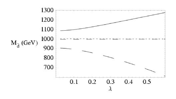
Figure 1: Physical masses of the $down$-type squarks as a function of $\lambda$ when all the SUSY mass parameters are equal to 1 $TeV$ and $\tan\beta=40$. The solid line corresponds to $M_{\tilde{d}_{1}}$ , the long dashed line corresponds to $M_{\tilde{d}_{4}}$ and the other two correspond to $M_{\tilde{d}_{2}}$ and $M_{\tilde{d}_{3}}$ (short-dashed and semi-short-dashed) respectively.

The numerical analysis for the up-type squarks is completely analogous to the previous one of the down-type squarks and we dont show it here explicitly. Concerning the mass pattern and its dependence with $\lambda$, there are two eigenvalues, $M_{\tilde{u}_{2}}$ and $M_{\tilde{u}_{3}}$ that do not change much as we increase the value of $\lambda$, and that correspond, when $\lambda=0$, to $\tilde{c}_{1}$ and $\tilde{c}_{2}$ respectively. On the other hand, $M_{\tilde{u}_{1}}$ increases with $\lambda$ while $M_{\tilde{u}_{4}}$ decreases and these last ones correspond, when $\lambda=0$, to $\tilde{t}_{1}$ and $\tilde{t}_{2}$ respectively.

Finally, notice that, for the numerical analysis of the FCHD rates in the next sections, only $\lambda$ values in the $0\leq\lambda\leq 1$ range that lead to physical squark masses above $150\,GeV$ will be considered. The present experimental lower mass bounds on the squark masses of the first and second squark generation are actually even more stringent that this value [34], but we have chosen here this common value of $150\,GeV$ for simplicity and definiteness. Similarly, in view of the present experimental lower bounds on the gluino mass [34], we will consider here $M_{\tilde{g}}$ values above $200\,GeV$.

The previously introduced intergenerational mixing effects in the squark sector lead to strong FC effects in processes involving neutral currents through the quark-squark-gluino interaction Lagrangian, which can now be written in the squark mass eigenstate basis as,

$$\mathcal{L}(\tilde{g},\tilde{q},q) = -\sqrt{2}g_{s}\mathtt{t}\left(R_{3\alpha}^{(u)*}\bar{\tilde{g}}\tilde{u}_{\alpha}^{*}t_{L}+R_{3\alpha}^{(d)*}\bar{\tilde{g}}\tilde{d}_{\alpha}^{*}b_{L}-R_{4\alpha}^{(u)*}\bar{\tilde{g}}\tilde{u}_{\alpha}^{*}t_{R}-R_{4\alpha}^{(d)*}\bar{\tilde{g}}\tilde{d}_{\alpha}^{*}b_{R}\right.$$

$$\left.+R_{1\alpha}^{(u)*}\bar{\tilde{g}}\tilde{u}_{\alpha}^{*}c_{L}+R_{1\alpha}^{(d)*}\bar{\tilde{g}}\tilde{d}_{\alpha}^{*}s_{L}-R_{2\alpha}^{(u)*}\bar{\tilde{g}}\tilde{u}_{\alpha}^{*}c_{R}-R_{2\alpha}^{(d)*}\bar{\tilde{g}}\tilde{d}_{\alpha}^{*}s_{R}\right)+h.c$$

with $\alpha=1,2,3,4$ and we have used the short notation $\mathtt{t}\bar{\tilde{g}}\tilde{q}^{*}q\equiv t_{ij}^{a}\bar{\tilde{g}}_{a}\tilde{q}^{*i}q^{j}$, where $t_{ij}^{a}$ are the standard $SU(3)_{c}$ generators. For simplicity, we will omit the color indices from now on.

In this way, if there is misalignment between quark and squarks, new FC effects will appear in neutral currents processes and, in particular, in the neutral Higgs decays of the MSSM into quarks that we are interested in. These will occur, mainly, via loops of squarks and gluinos and through the flavour non-diagonal $q-\tilde{q}-\tilde{g}$ couplings of eq.(LABEL:eq.gluinosqq) which in turn have emerged from the flavour non-diagonal squark squared mass matrices of eqs.(2.1) and (2.2). These effects will be driven by the strong coupling constant $\alpha_{S}$, and therefore they are expected to be numerically large. We will study those effects in full detail in the forthcoming sections 3, 4 and 5.

3 Generating flavour changing Higgs decays from squark-gluino loops

We present in this section the computation of the one-loop radiative corrections to the FCHD of the neutral MSSM Higgs bosons into second and third generation quarks, $H\to b\bar{s},s\bar{b},t\bar{c},c\bar{t}$. Notice that, the present theoretical upper mass bound $m{{}_{h_{o}}}\leq 135\,GeV$ [35] makes the lightest Higgs boson $h_{o}$ unable to decay into $t\bar{c}$ or $c\bar{t}$. Therefore, just the following channels will be considered, $H_{a}\to b\bar{s},s\bar{b}$ with $H_{a}=h_{o},H_{o},A_{o}$ and $H_{a}\to t\bar{c},c\bar{t}$ with $H_{a}=H_{o},A_{o}$. We will focus on the radiative corrections that come from the SUSY-QCD sector, and more specifically those from loops of squarks of type $\tilde{s}$, $\tilde{c}$, $\tilde{b}$ and $\tilde{t}$, and gluinos $\tilde{g}$. These will provide contributions to the FC partial widths of $\mathcal{O}(\alpha_{S}^{2})$ and are expected to be the dominant ones.

Notice that, the computation of these FC partial widths are relatively easy and do not require renormalization, because these decay processes do not proceed at the tree level in the MSSM. One just computes the different one-loop diagrams that contribute to the process and the final result obtained, after adding up all of them, must be finite, since no lowest order interaction could absorb the left over infinities.

In order to present our results for the partial decay widths, it is convenient to define the one-loop effective interaction term associated to each decay $H\to q\bar{q}^{\prime}$ in the following compact form:

$$iF=-ig\bar{u}_{q}(p_{1})(F_{L}^{qq^{\prime}}(H)P_{L}+F_{R}^{qq^{\prime}}(H)P_{R})v_{q^{\prime}}(p_{2})H(p_{3}),$$ (3.1)

where $g$ is the $SU(2)_{L}$ gauge coupling and $F_{L}$ and $F_{R}$ are the form factors associated to each chirality projection $L$ and $R$ respectively. The values of $F_{L}$ and $F_{R}$ follow from the explicit calculation of the one-loop vertices and mixed self-energies and are of order $\alpha_{S}$. These one-loop diagrams from the SUSY-QCD sector are depicted in fig.2 for the $H\to b\bar{s}$ decays, with $H=h_{o},H_{o},A_{o}$. The corresponding diagramas for the $tc$ decays are identical but replacing $d\to u$, $b\to t$ and $s\to c$.

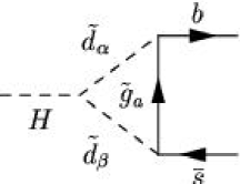
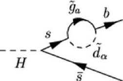
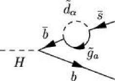
Figure 2: One-loop diagrams from the SUSY-QCD sector for the decay $H\to b\bar{s}$

For the mixed self-energy diagrams it is useful to define the following decomposition,

$$\Sigma^{bs}(k) = k{/}\Sigma_{L}^{bs}(k^{2})P_{L}+k{/}\Sigma_{R}^{bs}(k^{2})P_{R}+m_{b}(\Sigma_{Ls}^{bs}(k^{2})P_{L}+\Sigma_{Rs}^{bs}(k^{2})P_{R}),$$

and similarly for $\Sigma^{tc}(k)$ by replacing the quark flavour indices correspondingly, namely, $b\rightarrow t$ and $s\rightarrow c$.

By computing the diagrams in fig.2, we get the following results for the $d$-sector form factors in terms of the scalar one-loop integral functions $B_{0}$, $B_{1}$, $C_{0}$, $C_{11}$ and $C_{12}$, as defined in refs. [36],

$$F_{L}^{bs}(H_{a}) = -\frac{g_{H_{a}\tilde{d}_{\alpha}\tilde{d}_{\beta}}}{ig}\frac{2\alpha_{s}}{3\pi}\left(m_{b}R_{3\alpha}^{(d)}R_{1\beta}^{(d)*}(C_{11}-C_{12})+m_{s}R_{4\alpha}^{(d)}R_{2\beta}^{(d)*}C_{12}\right.$$ (3.3)

$$\left.+M_{\tilde{g}}R_{4\alpha}^{(d)}R_{1\beta}^{(d)*}C_{0}\right)(m_{b}^{2},m_{H_{a}}^{2},m_{s}^{2},M_{\tilde{g}}^{2},M_{\tilde{d}_{\alpha}}^{2},M_{\tilde{d}_{\beta}}^{2})$$

$$+\frac{G_{Hs\bar{s}}}{ig}\frac{m_{b}}{m_{b}^{2}-m_{s}^{2}}\kappa_{L}^{d}\left[m_{b}(\Sigma_{R}^{bs}(m_{b}^{2})+\Sigma_{Rs}^{bs}(m_{b}^{2}))+m_{s}(\Sigma_{L}^{bs}(m_{b}^{2})+\Sigma_{Ls}^{bs}(m_{b}^{2}))\right]$$

$$+\frac{G_{Hb\bar{b}}}{ig}\frac{1}{m_{s}^{2}-m_{b}^{2}}\kappa_{L}^{d}\left[m_{s}^{2}\Sigma_{L}^{bs}(m_{s}^{2})+m_{b}m_{s}(\Sigma_{Rs}^{bs}(m_{s}^{2})+\Sigma_{R}^{bs}(m_{s}^{2}))\right.$$

$$\left.+m_{b}^{2}\Sigma_{Ls}^{bs}(m_{s}^{2})\right]$$

$$F_{R}^{bs}(H_{a}) = -\frac{g_{H_{a}\tilde{d}_{\alpha}\tilde{d}_{\beta}}}{ig}\frac{2\alpha_{s}}{3\pi}\left(m_{b}R_{4\alpha}^{(d)}R_{2\beta}^{(d)*}(C_{11}-C_{12})+m_{s}R_{3\alpha}^{(d)}R_{1\beta}^{(d)*}C_{12}\right.$$ (3.4)

$$\left.+M_{\tilde{g}}R_{3\alpha}^{(d)}R_{2\beta}^{(d)*}C_{0}\right)(m_{b}^{2},m_{H_{a}}^{2},m_{s}^{2},M_{\tilde{g}}^{2},M_{\tilde{d}_{\alpha}}^{2},M_{\tilde{d}_{\beta}}^{2})$$

$$+\frac{G_{Hs\bar{s}}}{ig}\frac{m_{b}}{m_{b}^{2}-m_{s}^{2}}\kappa_{R}^{d}\left[m_{b}(\Sigma_{L}^{bs}(m_{b}^{2})+\Sigma_{Ls}^{bs}(m_{b}^{2}))+m_{s}(\Sigma_{R}^{bs}(m_{b}^{2})+\Sigma_{Rs}^{bs}(m_{b}^{2}))\right]$$

$$+\frac{G_{Hb\bar{b}}}{ig}\frac{1}{m_{s}^{2}-m_{b}^{2}}\kappa_{R}^{d}\left[m_{s}^{2}\Sigma_{R}^{bs}(m_{s}^{2})+m_{b}m_{s}(\Sigma_{Ls}^{bs}(m_{s}^{2})+\Sigma_{L}^{bs}(m_{s}^{2}))\right.$$

$$\left.+m_{b}^{2}\Sigma_{Rs}^{bs}(m_{s}^{2})\right].$$

Similarly, by computing the equivalent diagrams for the $tc$ decays, we find the expresions for the $u$-sector form factors, $F_{L}^{tc}(H_{a})$ and $F_{R}^{tc}(H_{a})$, which are identical to the previous results for $F_{L}^{bs}(H_{a})$ and $F_{R}^{bs}(H_{a})$ respectively, but replacing the flavour indices correspondingly, namely, $b\rightarrow t$, $s\rightarrow c$ and $d\rightarrow u$.

In the previous formulas, the $g_{H_{a}\tilde{q}_{\alpha}\tilde{q}_{\beta}}$ are the Higgs-squark-squark couplings in the mass eigenstate basis, which are collected in the Appendix A. The Higgs-quark-quark couplings are given by, $G_{Hq\bar{q}}=-\frac{igm_{q}}{2M_{W}\cos\beta}$, for $q=s,b$, and $G_{Hq\bar{q}}=-\frac{igm_{q}}{2M_{W}\sin\beta}$, for $q=c,t$. The $\kappa$ factors depend on the particular Higgs decay. These are, $\kappa_{L}^{u}=(\cos\alpha,\sin\alpha,i\cos\beta)$, $\kappa_{L}^{d}=(-\sin\alpha,\cos\alpha,i\sin\beta)$, and $\kappa_{R}^{(u,d)}=\kappa_{L}^{(u,d)*}$ for the decays of $H_{a}=(h_{o},H_{o},A_{o})$, respectively. The last parenthesis in the second line of all the form factors refer to the arguments of the one-loop $C_{0}$, $C_{11}$ and $C_{12}$ functions. Finally, the one-loop contributions from the SUSY-QCD sector to the mixed self-energies appearing in the previous equations are the following,

$$\Sigma_{L}^{tc,bs}(k^{2}) = -\frac{2\alpha_{s}}{3\pi}B_{1}(k^{2},M_{\tilde{g}}^{2},M_{\tilde{u}_{\alpha},\tilde{d}_{\alpha}}^{2})R_{3\alpha}^{(u,d)}R_{1\alpha}^{(u,d)*}$$

$$\Sigma_{R}^{tc,bs}(k^{2}) = -\frac{2\alpha_{s}}{3\pi}B_{1}(k^{2},M_{\tilde{g}}^{2},M_{\tilde{u}_{\alpha},\tilde{d}_{\alpha}}^{2})R_{4\alpha}^{(u,d)}R_{2\alpha}^{(u,d)*}$$

$$m_{t,b}\Sigma_{Ls}^{tc,bs}(k^{2}) = -\frac{2\alpha_{s}}{3\pi}M_{\tilde{g}}B_{0}(k^{2},M_{\tilde{g}}^{2},M_{\tilde{u}_{\alpha},\tilde{d}_{\alpha}}^{2})R_{4\alpha}^{(u,d)}R_{1\alpha}^{(u,d)*}$$

$$m_{t,b}\Sigma_{Rs}^{tc,bs}(k^{2}) = -\frac{2\alpha_{s}}{3\pi}M_{\tilde{g}}B_{0}(k^{2},M_{\tilde{g}}^{2},M_{\tilde{u}_{\alpha},\tilde{d}_{\alpha}}^{2})R_{3\alpha}^{(u,d)}R_{2\alpha}^{(u,d)*}$$ (3.5)

The expressions for the form factors involved in the $H_{a}\to c\bar{t},\,t\bar{c}$ decays have been checked to be in agreement with the previous results obtained in [26] for the $t\to cH_{a}$ decays.

We next present the results of the partial decay widths for the decays $H_{a}\to t\bar{c},c\bar{t}$ where $H_{a}=H_{o},A_{o}$ and $H_{a}\to b\bar{s},s\bar{b}$ where $H_{a}=h_{o},H_{o},A_{o}$, in terms of the above form factors. Since we are assuming that the final states $q\bar{q}^{\prime}$ and $q^{\prime}\bar{q}$ are not experimentally distinguishable, the final results for the total partial widths are got by adding the two corresponding partial widths, and this will be denoted from now on by $\Gamma(H\to q\bar{q}^{\prime}+q^{\prime}\bar{q})$. These results are as follows,

$$\Gamma(H_{a}\to b\bar{s}+s\bar{b}) = \frac{2g^{2}}{16\pi m_{H_{a}}}\lambda^{\frac{1}{2}}\left(1,\frac{m_{s}^{2}}{m_{H_{a}}^{2}},\frac{m_{b}^{2}}{m_{H_{a}}^{2}}\right)\times$$

$$\left[3(m_{H_{a}}^{2}-m_{s}^{2}-m_{b}^{2})(F_{L}^{bs}(H_{a})F_{L}^{bs*}(H_{a})+F_{R}^{bs}(H_{a})F_{R}^{bs*}(H_{a}))\right.$$

$$\left.-6m_{b}m_{s}(F_{L}^{bs}(H_{a})F_{R}^{bs*}(H_{a})+F_{R}^{bs}(H_{a})F_{L}^{bs*}(H_{a}))\right]$$

$$\Gamma(H_{a}\to t\bar{c}+c\bar{t}) = \frac{2g^{2}}{16\pi m_{H_{a}}}\lambda^{\frac{1}{2}}\left(1,\frac{m_{c}^{2}}{m_{H_{a}}^{2}},\frac{m_{t}^{2}}{m_{H_{a}}^{2}}\right)\times$$ (3.7)

$$\left[3(m_{H_{a}}^{2}-m_{c}^{2}-m_{t}^{2})(F_{L}^{tc}(H_{a})F_{L}^{tc*}(H_{a})+F_{R}^{tc}(H_{a})F_{R}^{tc*}(H_{a}))\right.$$

$$\left.-6m_{t}m_{c}(F_{L}^{tc}(H_{a})F_{R}^{tc*}(H_{a})+F_{R}^{tc}(H_{a})F_{L}^{tc*}(H_{a}))\right]$$

where $\lambda^{\frac{1}{2}}\left(1,x^{2},y^{2}\right)=\sqrt{\left[1-(x+y)^{2}\right]\left[1-(x-y)^{2}\right]}$. Notice again that, due to phase space, the lightest Higgs boson $h_{o}$ cannot decay into $t\bar{c}$ or $c\bar{t}$.

Some comments are in order. First, we have checked explicitly that the previous results for the form factors are finite, as expected. Second, we can see that the parameter $\lambda$, which characterizes the FC, does not appear explicitly in eqs.(3.3) and (3.4), but it appears implicitly. As we have already explained, the effect of FC is due to misalignment between the quark and squark mass matrices and is parametrized through non-diagonal terms in the squark squared mass matrices containing the parameter $\lambda$. Therefore, the dependence on $\lambda$ is hidden in the respective rotation matrices used to diagonalize the squark squared mass matrices, $R_{\alpha\beta}^{(u)}$ and $R_{\alpha\beta}^{(d)}$, and obviously in the physical squark mass values, which appear as arguments of the scalar one-loop integral functions obtained in the one-loop calculation.

On the other hand, the MSSM parameters $\tan\beta$, $\mu$ and $M_{\tilde{g}}$ will be crucial for our phenomenological analysis of section 4, where we will study numerically the size of these loop induced FCHD as a function of these MSSM parameters. The dependence on $\mu$ and $\tan\beta$ in the form factors, and hence, in the decay widths, is complicated and is hidden inside couplings and inside the squark mass matrices. $M_{\tilde{g}}$ appears as an argument of the scalar one-loop integral functions, and also it appears explicitly as a multiplicative factor in both the vertex $C_{0}$ contributions and the scalar parts of the mixed self-energy diagrams. The global dependence on the angle $\beta$ is more complicated, as it emerges in most of the terms. The explicit $\beta$ dependence through $LR$ flavour preserving squark mixing, namely, $m_{b,s}(A_{b,s}-\mu\tan\beta)$ and $m_{t,c}(A_{t,c}-\mu\cot\beta)$, shows that the contribution from these mixing terms in the $down$ sector grows with $\tan\beta$ and its dependence on $A_{b,s}$, for large values of $\tan\beta$, is expected to be mild, while in the $up$ sector, it is less $\tan\beta$ dependent for $\tan\beta>1$ and the trilinear term, $A_{t,c}$, can acquire more importance.

At the end, one crucial parameter for our complete analysis will be $\mu$, which appears in the squark mass matrix term in the way exposed above, but also, directly in the Higgs-squark-squark couplings, as can be seen in the Appendix A. As we will show in the next sections, large values of $\mu$ can produce sizable contributions to FCHD.

All these complicated dependences with the different MSSM parameters will be clarified in the analysis performed in the next section, and the analytical behaviour will be explained in more detail in the large SUSY mass limit performed in section 5, where we study the behaviour of these FC decay processes in the scenario where a very heavy supersymmetric spectrum is considered.

4 Numerical Analysis of the FCHD rates

In this section we estimate numerically the size of the loop induced FCHD as a function of the MSSM parameters and the $\lambda$ parameter. The MSSM parameters needed to fully characterize and evaluate the $\Gamma(H_{a}\to b\bar{s}+s\bar{b})$ and $\Gamma(H_{a}\to t\bar{c}+c\bar{t})$ partial widths, in our simplified scenario, consist of the following six parameters: $m_{A}$, $\tan\beta$, $\mu$, $M_{\tilde{g}}$, $M_{o}$, and A, where we have chosen, for simplicity, $M_{o}$ as a common value for the soft squark breaking mass parameters, $M_{o}=M_{\tilde{Q},q}=M_{\tilde{U},(c,t)}=M_{\tilde{D},(s,b)}$, and all the various trilinear parameters to be equal $A_{t}=A_{b}=A_{c}=A_{s}=A$. These parameters will be varied over a broad range, subject only to our requirement that all the squark masses be heavier than 150 $GeV$, and that the gluino mass be heavier than $200\,GeV$. On the other hand, the extra parameter, $\lambda$, which is the only one measuring the FC strength, will be varied in the range $0\leq\lambda\leq 1$, and only values leading to $M_{\tilde{q}}>150\,GeV$ will be considered.

In order to estimate the FCHD rates over the MSSM parameter space and the $\lambda$ interval chosen, and with the motivation in mind of finding the region of the MSSM parameter space where these rates are maximal, we will proceed as follows. We will first fix the $\lambda$ parameter to one concrete value in the range $0\leq\lambda\leq 1$ and vary the rest of parameters over the whole allowed range in order to detect such maximizing region. Next, we will fix all the MSSM parameters to some specific values belonging to this region and study the widths and branching ratios as a function of the $\lambda$ parameter. This will give us finally the maximum size of these observables as a function of $\lambda$ as well, and if any planned experiment is able to observe and measure these FCHD rates with good accuracy, their experimental value could serve to extract either the preferred $\lambda$ value or, in the worst case, an upper bound on it.

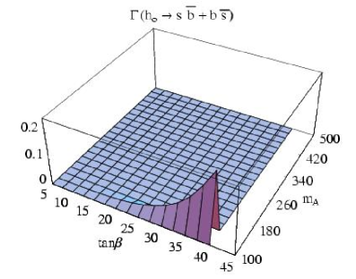
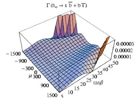
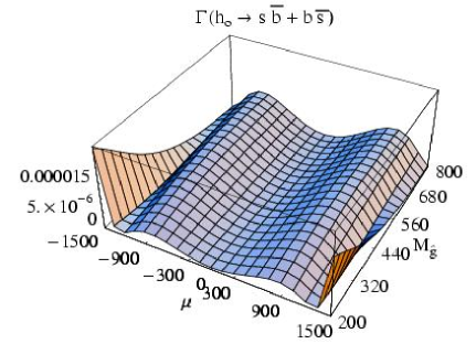
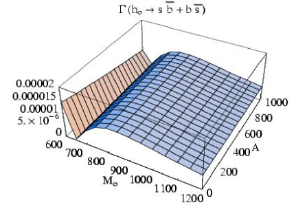
Figure 3: $\Gamma(h_{o}\to b\bar{s}+s\bar{b})$ in $GeV$ as a function of ($\tan\beta$, $m_{A}$ ($GeV$)) (a), ($\mu$ ($GeV$), $\tan\beta$) (b), ($\mu$ ($GeV$), $M_{\tilde{g}}$ ($GeV$)) (c) and ($M_{o}$ ($GeV$), $A$ ($GeV$)) (d). The regions of the parameter space not plotted are the ones that give non allowed values for the squark masses ($M_{\tilde{q}}<150\,GeV$). The values of the different MSSM parameters that have to be fixed in each plot have been chosen correspondingly to be: $\mu=1500\,GeV$, $M_{o}=600\,GeV$, $M_{\tilde{g}}=300\,GeV$, $A=200\,GeV$, $m_{A}=250\ GeV$, $\tan\beta=35$ and $\lambda=0.5$.

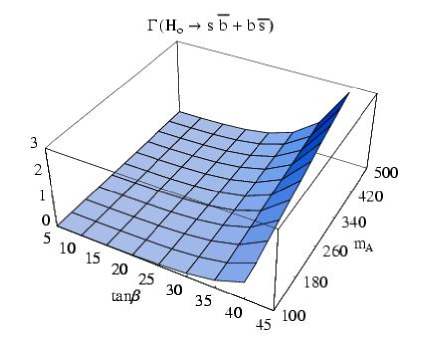
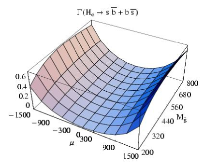
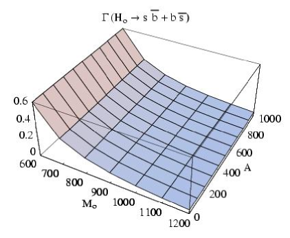
Figure 4: Same as in fig.3 but for $\Gamma(H_{o}\to b\bar{s}+s\bar{b})$.

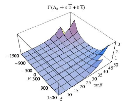
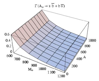
Figure 5: Same as in fig.3 but for $\Gamma(A_{o}\to b\bar{s}+s\bar{b})$.

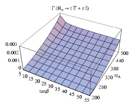
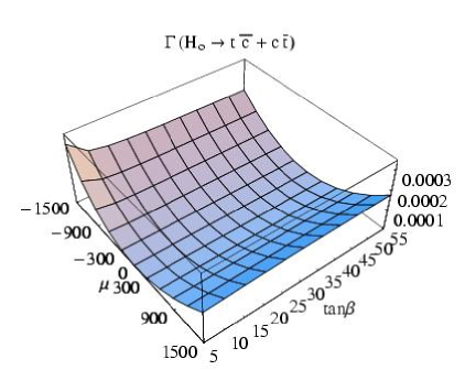
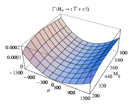
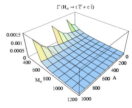
Figure 6: $\Gamma(H_{o}\to t\bar{c}+c\bar{t})$ in $GeV$ as a function of ($\tan\beta$, $m_{A}$ ($GeV$)) (a), ($\mu$ (GeV), $\tan\beta$) (b), ($\mu$ ($GeV$), $M_{\tilde{g}}$ ($GeV$)) (c) and ($M_{o}$ ($GeV$), $A$ ($GeV$)) (d). The regions of the parameter space not plotted are the ones that give non allowed values for the squark masses ($M_{\tilde{q}}<150\,GeV$). The values of the different MSSM parameters that have to be fixed in each plot have been chosen correspondingly to be: $\mu=-1500\,GeV$, $M_{o}=600\,GeV$, $M_{\tilde{g}}=500\,GeV$, $A=800\,GeV$, $m_{A}=250\,GeV$ and $\tan\beta=10$.

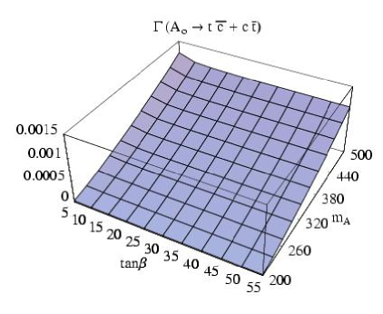
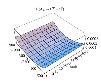
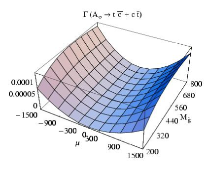
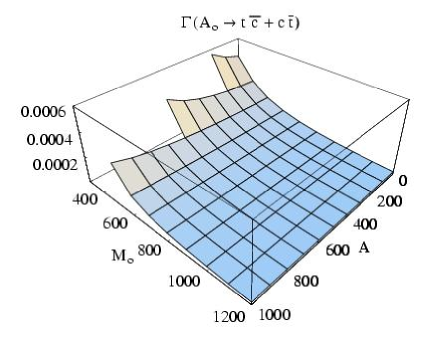
Figure 7: Same as in fig.6 but for $\Gamma(A_{o}\to t\bar{c}+c\bar{t})$.

The figs.3 through 7 display the numerical results for the $\Gamma(H_{a}\to b\bar{s}+s\bar{b})$ and $\Gamma(H_{a}\to t\bar{c}+c\bar{t})$ partial widths as a function of the six previous MSSM parameters, $m_{A}$, $\tan\beta$, $\mu$, $M_{\tilde{g}}$, $M_{0}$ and $A$, and for the specific value $\lambda=0.5$. In these figures, the MSSM parameters have been grouped in pairs in order to illustrate simultaneously the behaviour of the FCHD widths with both parameters. These pairs of parameters have been chosen to be: ($\tan\beta$, $m_{A}$), ($\mu$, $\tan\beta$), ($\mu$, $M_{\tilde{g}}$) and ($M_{o}$, $A$), and correspond to the plots (a) (upper left panel), (b) (upper right panel), (c) (lower left panel) and (d) (lower right panel), respectively, in these figures. We have made these four plots for each neutral Higgs boson. figs.3, 4 and 5 correspond to $\Gamma(h_{o}\to b\bar{s}+s\bar{b}),\,\Gamma(H_{o}\to b\bar{s}+s\bar{b})$ and $\Gamma(A_{o}\to b\bar{s}+s\bar{b})$, respectively, and figs.6 and 7 correspond to $\Gamma(H_{o}\to t\bar{c}+c\bar{t})$ and $\Gamma(A_{o}\to t\bar{c}+c\bar{t})$, respectively. Notice again that the lightest Higgs cannot decay to $t\bar{c}$ nor $c\bar{t}$, due to phase space.

In the following we discuss separately the $\Gamma(H_{a}\to b\bar{s}+s\bar{b})$ and $\Gamma(H_{a}\to t\bar{c}+c\bar{t})$ cases due to their different behaviour with some of the MSSM parameters.

First, we will focus on $\Gamma(H_{a}\to b\bar{s}+s\bar{b})$ (see figs.3, 4 and 5, for the $h_{o}$, $H_{o}$ and $A_{o}$ respectively). Let us start with the first plot, (a), of these figures where we study the combined behaviour with $\tan\beta$ and $m_{A}$. The first clear behaviour of these decay widths is the fast growing with $\tan\beta$. Notice that it is the same behaviour for the three neutral Higgs bosons, despite the fact that the growing with $\tan\beta$ is better seen in the case of the $H_{o}$ and $A_{o}$ than in the lightest Higgs one, due only to the different scales shown. It is important to recall that there are some values of the widths that are not shown in the figures since they correspond to non allowed values for the squark masses, that is $M_{\tilde{q}}<150\,GeV$. In particular, in this first plot we can see that for the values of the parameters specified in the figure caption, values of about $\tan\beta>40$ are not allowed in order to keep the squarks masses in the allowed region. Keeping this in mind and the growing behaviour with $\tan\beta$, we can conclude that the searched parameter space region that maximizes the FC effect is localized at large $\tan\beta$ values, with the largest possible values being constrained to be below some maximum, which depends on the particular values of the other parameters.

We next study the behaviour with $m_{A}$. We see again from plot (a) of each figure that it is clearly different, depending on the particular Higgs decay we are studying. The decay widths $\Gamma(H_{o}\to b\bar{s}+s\bar{b})$ and $\Gamma(A_{o}\to b\bar{s}+s\bar{b})$ clearly grow with $m_{A}$ due to the obvious phase space effects, that is, as $m_{A}$ increases, the corresponding Higgs mass increases too. In contrast, the $\Gamma(h_{o}\to b\bar{s}+s\bar{b})$ width shows a less obvious behaviour with $m_{A}$. As the lightest Higgs mass starts growing with $m_{A}$ and then it stabilizes, its decay width first grows with $m_{A}$, then it reaches a maximum value and finally decreases with $m_{A}$, and we appreciate the setting of the decoupling behaviour for large $m_{A}$ values that will be better explained in section 5.

The phenomenologically interesting $m_{A}$ values would be those that can allow the next planned colliders to detect and study all the three neutral Higgs bosons. For definiteness, in our numerical analysis whenever we have to fix $m_{A}$, we have chosen $m_{A}=250\,GeV$, which for the interesting large $\tan\beta$ region, gives the three boson masses $m_{h_{o}}$, $m_{H_{o}}$, and $m_{A}$ being accessible to the LHC. On the other hand, regarding particularly the lightest Higgs, as it is the one that has more possibilities of being detected in the next years, it would be also interesting to further study the region of lower $m_{A}$ values but we do not explore this here.

Now we focus on the behaviour with $\mu$. We can clearly see in figs.3, 4 and 5, (b) and (c), that the widths are approximately symmetric under $\mu\to-\mu$ and that for moderate $|\mu|<600\,GeV$ they all grow with this parameter. We can appreciate this growing behaviour in all the flavour changing Higgs decays. The $H_{o}$ and $A_{o}$ decay widths grow with $|\mu|$ for all $\mu$ values, (figs.4 and 5 (b) and (c)); but the lightest Higgs decay first grows with $|\mu|$ from $\mu=0$, then, it reaches a maximum, decreases up to a minimum, and finally it continues growing (fig.3 (b) and (c)). We have found that this particular behaviour of the lightest Higgs boson is due to an accidental numerical cancellation among the contributions from the different diagrams to the form factors, $F_{L}^{bs}(h_{o})$ and $F_{R}^{bs}(h_{o})$, which takes place in this decay and not in the rest of decays under study.

On the other hand, this behaviour with $\mu$, as can be seen in figs.(3, 4 and 5 (b)), depends also strongly on $\tan\beta$, because these two parameters appear together in the squark mixings, and the behaviour of the widths with them are correlated. For large $\tan\beta$ they grow faster with $\mu$, and for small $\tan\beta$ the trilinear term starts to play a role too, so this growing smoothes down. Due to this correlation, one has to be careful in choosing independently both parameters as this could lead to non allowed values of the squark masses, $M_{\tilde{q}}<150\,GeV$. In particular, we can see again in plots (b), how for large values of the $\mu$ parameter, as for instance $\mu=1500\,GeV$, only $\tan\beta$ values below about 40 are allowed.

Following with $M_{\tilde{g}}$ (figs.3, 4 and 5 (c)), we find that the FC widths grow with $M_{\tilde{g}}$ up to a certain value $M_{\tilde{g}_{o}}$ and then they decrease very slowly (slow decoupling). Clearly, the value of $M_{\tilde{g}_{o}}$ depends on the rest of parameters. For the explored MSSM parameter space region, we can see from these figures that it is in the range between about $200\,GeV$ and $800\,GeV$.

On the other hand, the behaviour with $M_{o}$ is very clear too (figs.3, 4 and 5 (d)). All the decay widths decrease with this parameter, for large $M_{o}$, as it was expected. When $M_{o}$ grows, the masses of the squarks inside the loops grow as well, thus the probability of producing such loop-induced processes decreases as they are suppressed by the squark masses in the propagators.

To finish, we can see as well in figs. (d) that the partial widths in the $d$-sector are nearly independent of the trilinear parameters $A$ for all the studied decays.

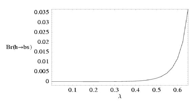
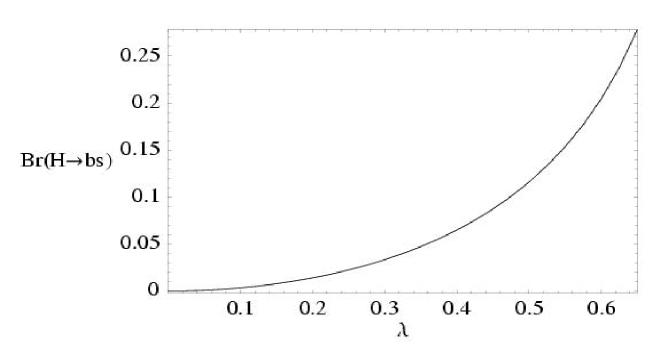
Figure 8: $Br(H_{a}\to b\bar{s}+s\bar{b})$, $H_{a}=(h_{o},H_{o},A_{o})$ as a function of $\lambda$ for the selected MSSM parameters. $Br(A_{o}\to b\bar{s}+s\bar{b})$ is not plotted explicitly since in this range of the parameter space is undistinguisable from the $H_{o}$ decay. Higher values of $\lambda$ are not allowed as they give $M_{\tilde{q}}<150\,GeV$.

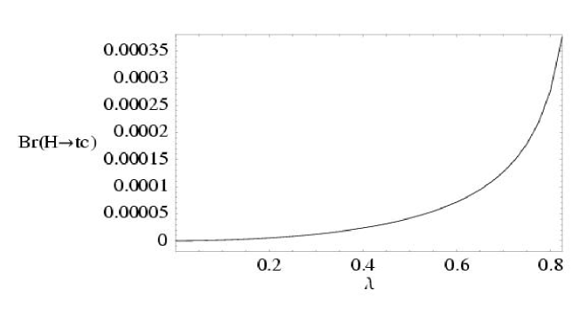
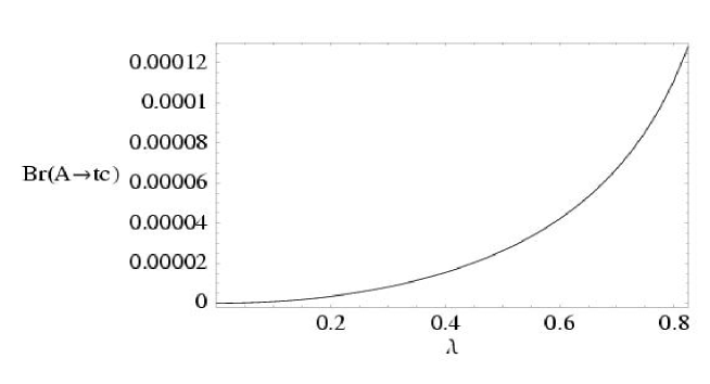
Figure 9: $Br(H_{a}\to t\bar{c}+c\bar{t})$, $H_{a}=(H_{o},A_{o})$ as a function of $\lambda$ for the selected MSSM parameters. Higher values of $\lambda$ are not allowed as they give $M_{\tilde{q}}<150\,GeV$.

In the following we will discuss the decay widths $\Gamma(H_{a}\to t\bar{c}+c\bar{t})$ (figs.6 and 7), where, as we have already explained, we will only study the behaviour of $H_{o}$ and $A_{o}$ decays, as the lightest Higgs cannot decay to $t\bar{c}$ or $c\bar{t}$.

Again, the first plot (a) of each figure represents the combined behaviour of the decay widths with $\tan\beta$ and $m_{A}$. One of the fundamental differences among these decays of the $u$-sector and the ones studied before of the $d$-sector is that now there is a very mild dependence with $\tan\beta$ and the widths decrease softly with $\tan\beta$. Therefore, this time, the value that maximizes our effect is the smallest $\tan\beta$ value, but as we have said, the numerical effect of this parameter is not of crucial importance in these decays.

Regarding the behaviour with $m_{A}$, as can be seen in figs.6 and 7 (a), it does not vary much with respect to the previous ones. The decay widths of the $H_{o}$ and $A_{o}$ again grow with $m_{A}$ due to the phase space as explained above, thus the same motivations to select a particular $m_{A}$ value will apply here.

The partial widths again grow with $\mu$ and are approximately symmetric under $\mu\to-\mu$, but they show less symmetry than in the decays of the $d$-quark sector studied earlier. The squark mixing term now goes with $m_{t,c}(A_{t,c}-\mu\cot\beta)$ so the trilinear parameter $A$ becomes more important for $\tan\beta>1$. Looking at the plots 6 and 7 (b), (c) we can see that the maximum values are reached for negative values of $\mu$. We see as well that for large values of $\mu$ we can better appreciate the $\tan\beta$ dependence.

Looking at the behaviour of the partial widths in the $u$-quark sector with the gluino mass, $M_{\tilde{g}}$, in figs.6 and 7 (c), the widths again grow with $M_{\tilde{g}}$ until they reach a maximum at a certain value $M_{\tilde{g}_{o}}$, and then they start a slow decreasing (slow decoupling), as in the case of the $d$-quark sector studied above. Again, the value of $M_{\tilde{g}_{o}}$ also depends on the rest of parameters, and the mentioned behaviour is more evident for large values of the parameter $\mu$.

The behaviour with $M_{o}$ is again the same as before, decreasing with it as it was expected, but now, the trilinear parameter $A$ acquires more importance than before, growing the flavour changing widths as we increase the value of $A$. Again here, it is worth mentioning that there are some values not being plotted that correspond to non allowed values for the squark masses. In particular, for small values of $M_{o}$, only small values of $A$ are allowed. As a particular example, looking at figs.6 and 7 (d) we can see that for $M_{o}=400\,GeV$, values of the trilinear parameter $A$ larger than about $600\,GeV$ would not be allowed.

Finally, we study the behaviour of the corresponding FCHD branching ratios with $\lambda$, and estimate their size for $0\leq\lambda\leq 1$ and for some selected points of the MSSM parameter space, which have been chosen belonging to the region where the FC effects we are looking for are maximized. This region can be extracted easily from our results in the previous figures. Thus, for the $H_{a}\to b\bar{s},s\bar{b}$ decays we select the following representative point: $m_{A}=250\,GeV$, $\tan\beta=35$, $\mu=1500\,GeV$, $M_{\tilde{g}}=300\,GeV$, $M_{0}=600\,GeV$ and $A=200\,GeV$; and for the $H_{a}\to t\bar{c},c\bar{t}$ decays we choose: $m_{A}=250\,GeV$, $\tan\beta=10$, $\mu=-1500\,GeV$, $M_{\tilde{g}}=500\,GeV$, $M_{0}=600\,GeV$ and $A=800\,GeV$. Regarding the computation of the total Higgs boson widths, these have been evaluated with the HDECAY program [37].

For the $H_{a}\to b\bar{s},s\bar{b}$ decays, as can be seen in fig.8, the branching ratios grow with $\lambda$, being exactly zero for $\lambda=0$, as expected, and can reach quite sizeable values, even for moderate $\lambda$. For instance, for $\lambda\approx 0.6$ the branching ratio for the $h_{o}$ is about $0.015$, and for the $A_{o}$ and $H_{o}$ is about $0.25$. Of course, larger $\lambda$ values would lead to larger rates, but these are not allowed here due to the $M_{\tilde{q}}>150\,GeV$ restriction.

For the $H_{a}\to t\bar{c},\,c\bar{t}$ decays, as can be seen in fig.9, the branching ratios grow again with $\lambda$, being exactly zero for $\lambda=0$. Again, only $\lambda$ values leading to $M_{\tilde{q}}>150\,GeV$ are shown. The $H_{o}$ branching ratio reaches its maximum value, of about 0.00035 for $\lambda\approx 0.8$, while the pseudoscalar branching ratio reaches 0.0001 for this same value of $\lambda$.

In summary, the FCHD branching ratios that we have found in this section are quite sizable, in fact, many orders of magnitude larger that the corresponding SM rates (for instance, in the $u$-sector, and for $m_{H_{SM}}=200\,GeV$ we estimate $B(H_{SM}\to t\bar{c}+c\bar{t})\sim 10^{-13})$ and will produce an interesting amount of rare events at the planned next generation colliders. We do not study here this in more detail and postpone this interesting analysis for a future work.

5 Non-Decoupling Behaviour of Heavy Squarks and Gluinos in Flavour Changing Higgs Decays

In the previous sections we have studied the FC effects of squarks and gluinos via SUSY-QCD radiative corrections in the decays of neutral Higgs particles within the MSSM. We have performed analytical and numerical calculations, and estimated the size of these effects as a function of the various MSSM parameters and $\lambda$. In this section, we study the behaviour of these FCHD processes in the most pessimistic scenario where a heavy supersymmetric spectrum is considered, and we will show that these FC effects remain sizable even for squark and gluino masses as large as $\mathcal{O}(1TeV)$. We will show that the reason for these corrections remaining so large is that at asymptotically large SUSY particle masses they manifest a non-decoupling behaviour. That is, the one loop SUSY-QCD radiative corrections to the neutral MSSM Higgs boson decays remain non-vanishing at asymptotically large squark and gluino masses, and it results in a finite and non-negligible contribution which in principle could provide an indirect signal of SUSY-QCD at low energies, even in this pessimistic scenario.

The decoupling of all SUSY particles would imply that the prediction in the MSSM for all the observables involving non-SUSY particles in the external legs, such as the partial decay widths under study here, should tend, in the limit of large SUSY masses, to their corresponding values in the non-SUSY two Higgs doublet model, called 2HDMII in the literature [38]. Formally, and following the lines of the Appelquist-Carazzone Theorem [39], the decoupling would occur if the contributions of the SUSY particles to low-energy processes either fall as inverse powers of the SUSY mass parameters or can be absorbed into redefinitions of the couplings and parameters of the low-energy theory. In the present case, the decoupling of SUSY particles in the FCHD would imply, in particular, that the SUSY-QCD induced radiative corrections should tend to zero in the asymptotic large SUSY mass limit. This theorem has been proved to be valid for theories with an exact gauge symmetry, however, it does not apply to theories with spontaneously broken gauge symmetries, nor with chiral fermions, as it is clearly the case of the MSSM. Furthermore, in order to have decoupling, the dimensionless couplings should not grow with the heavy masses. Otherwise, the mass suppression induced by the heavy-particle propagators can be compensated by the mass enhancement provided by the interaction vertices, with an overall non-vanishing effect, which is exactly what happens in some Higgs boson decays to fermions. This has been proved to happen in some flavour preserving MSSM neutral Higgs boson decays in a series of previous works [40, 41, 42, 43, 44, 45] and also in $H^{+}$ production at hadronic colliders [46]. Here we will show that the non-decoupling effects also appear in the FCHD. These non-decoupling effects can have interesting phenomenological consequences as they imply that low-energy experiments can be sensitive to large mass scales, which cannot be kinematically accessed by direct searches.

In order to show analitically the non-decoupling behaviour of squarks and gluinos in the FCHD, we perform a systematic expansion of the form factors involved, and hence of the partial widths, in inverse powers of the heavy SUSY masses and look for the first term in this expansion. To define our expansion parameter, we consider here the simplest hypothesis where all the soft-SUSY-breaking mass parameters and the $\mu$ parameter are all of the same order (collectively denoted by $M_{S}$) and much heavier than the electroweak scale, $M_{EW}$, in such a way that the differences between these mass parameters are considered to be of order $M_{EW}$. That is,

$$M_{S}\simeq M_{o}\simeq M_{\tilde{g}}\simeq\mu\simeq A\gg M_{EW}$$ (5.1)

where again $M_{o}$ denotes the common soft breaking squark mass parameter, $M_{o}=M_{\tilde{Q}}=M_{\tilde{U}}=M_{\tilde{D}}$, and $M_{\tilde{Q}}$, $M_{\tilde{U}}$ and $M_{\tilde{D}}$ are chosen here, for simplicity, to be the same for the two generations involved, and $A$ is the common trilinear parameter. Notice that, with $M_{S}\sim\mathcal{O}(1TeV)$, this choice will lead to a plausible situation where all the SUSY particles in the SUSY-QCD sector are much heavier than their SM partners.

In the following, we perform the expansions of the SUSY-QCD contributions to the form factors, whose exact analytical results where presented in the previous section, in inverse powers of $M_{S}$ and keep just the leading contribution of this expansion by considering that all the remaining involved mass scales $m_{H_{o}},m_{A},m_{h_{o}},m_{Z},m_{W}$ and $m_{q}$ are of order $M_{EW}$. To this end, we use the results of the expansions of the one-loop functions and the rotation matrices that are given in Appendix B.

For the $H_{a}\to b\bar{s},\,s\bar{b}$ decays, with $H_{a}=h_{o},H_{o},A_{o}$, we find the following results for the leading terms in the expansions of the form factors,

$$F_{L}^{bs}(h_{o}) = \frac{\alpha_{s}}{6\pi}\frac{m_{b}\sin\alpha}{2m_{W}\cos\beta}(\tan\beta+\cot\alpha)\frac{\mu M_{\tilde{g}}}{M_{0}^{2}}F(\lambda)$$

$$F_{R}^{bs}(h_{o}) = \frac{\alpha_{s}}{6\pi}\frac{m_{s}\sin\alpha}{2m_{W}\cos\beta}(\tan\beta+\cot\alpha)\frac{\mu M_{\tilde{g}}}{M_{0}^{2}}F(\lambda)$$

$$F_{L}^{bs}(H_{o}) = -\frac{\alpha_{s}}{6\pi}\frac{m_{b}\cos\alpha}{2m_{W}\cos\beta}(\tan\beta-\tan\alpha)\frac{\mu M_{\tilde{g}}}{M_{0}^{2}}F(\lambda)$$

$$F_{R}^{bs}(H_{o}) = -\frac{\alpha_{s}}{6\pi}\frac{m_{s}\cos\alpha}{2m_{W}\cos\beta}(\tan\beta-\tan\alpha)\frac{\mu M_{\tilde{g}}}{M_{0}^{2}}F(\lambda)$$

$$F_{L}^{bs}(A_{o}) = -i\frac{\alpha_{s}}{6\pi}\frac{m_{b}}{2m_{W}}\tan\beta(\tan\beta+\cot\beta)\frac{\mu M_{\tilde{g}}}{M_{0}^{2}}F(\lambda)$$

$$F_{R}^{bs}(A_{o}) = i\frac{\alpha_{s}}{6\pi}\frac{m_{s}}{2m_{W}}\tan\beta(\tan\beta+\cot\beta)\frac{\mu M_{\tilde{g}}}{M_{0}^{2}}F(\lambda)$$ (5.2)

Similarly, for the $H_{a}\to t\bar{c},\,c\bar{t}$ decays, with $H_{a}=H_{o},A_{o}$, we find the following results for the leading terms in the expansions of the form factors,

$$F_{L}^{tc}(H_{o}) = -\frac{\alpha_{s}}{6\pi}\frac{m_{t}\sin\alpha}{2m_{W}\sin\beta}(\cot\beta-\cot\alpha)\frac{\mu M_{\tilde{g}}}{M_{0}^{2}}F(\lambda)$$

$$F_{R}^{tc}(H_{o}) = -\frac{\alpha_{s}}{6\pi}\frac{m_{c}\sin\alpha}{2m_{W}\sin\beta}(\cot\beta-\cot\alpha)\frac{\mu M_{\tilde{g}}}{M_{0}^{2}}F(\lambda)$$

$$F_{L}^{tc}(A_{o}) = -i\frac{\alpha_{s}}{6\pi}\frac{m_{t}}{2m_{W}}\cot\beta(\tan\beta+\cot\beta)\frac{\mu M_{\tilde{g}}}{M_{0}^{2}}F(\lambda)$$

$$F_{R}^{tc}(A_{o}) = i\frac{\alpha_{s}}{6\pi}\frac{m_{c}}{2m_{W}}\cot\beta(\tan\beta+\cot\beta)\frac{\mu M_{\tilde{g}}}{M_{0}^{2}}F(\lambda)$$ (5.3)

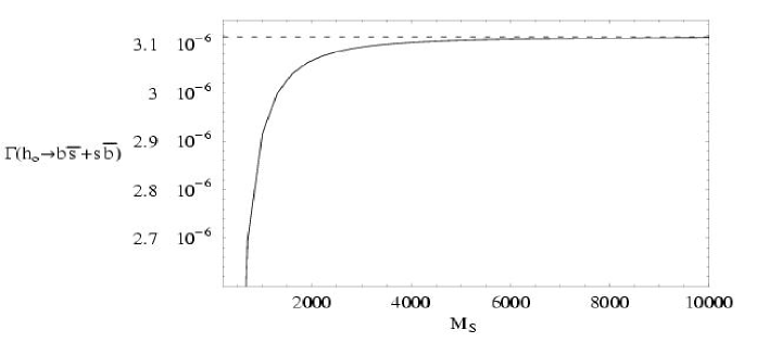
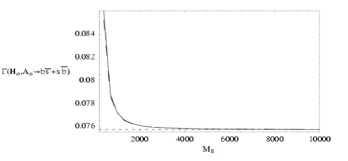
Figure 10: Non-decoupling behaviour of $\Gamma(H_{a}\to b\bar{s}+s\bar{b})$ in $GeV$ with $M_{0}=\mu=A=M_{\tilde{g}}=M_{S}$, for $H_{a}=h_{o}$ (top panel) and $H_{a}=H_{o},A_{o}$ (bottom panel) and for $\tan\beta=35$, $\lambda=0.5$, $m_{A}=m_{H_{o}}=250\,GeV$ and $m_{h_{o}}=135\,GeV$. Exact one-loop results in solid lines for the $h_{o}$ and $H_{o}$, long-dashed lines for the $A_{o}$. The expansions given in eq.(5.2) (short-dashed) are plotted for comparison.

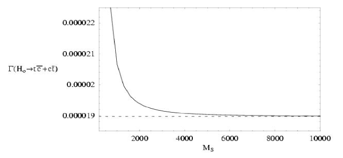
Figure 11: Non-decoupling behaviour of $\Gamma(H_{o}\to t\bar{c}+c\bar{t})$ in $GeV$ with $M_{0}=\mu=A=M_{\tilde{g}}=M_{S}$ and for $\tan\beta=35$, $\lambda=0.5$ and $m_{H_{o}}=250\,GeV$. Exact one-loop results (solid) and the expansions given in eq.(5.3) (short-dashed lines) are plotted for comparison. $\Gamma(A_{o}\to t\bar{c}+c\bar{t})$ is not plotted explicitly since in this range of the parameter space is undistinguisable from the $H_{o}$ decay.

Some comments are in order. First, we can see from eqs.(5.2) and (5.3) that, taking all SUSY mass parameters arbitrarily large and of the same order, the SUSY-QCD contributions to the FCHD partial widths lead to a non-zero value. That is, they do not decouple in the large SUSY mass scenario. This can be seen clearly, for instance, in the simplest case of equal mass scales, $\mu=M_{\tilde{g}}=M_{0}$, in which the dependence on the SUSY mass scale of the leading contributions disappear, and these provide a constant and non-vanishing value.

In the above eqs.(5.2) and (5.3) there appear one new function that is defined as,

$$F(\lambda)=\frac{2}{\lambda^{2}}[(\lambda+1)\ln(\lambda+1)+(\lambda-1)\ln(1-\lambda)-2\lambda],$$ (5.4)

where $\lambda$ is the parameter introduced in eqs.(2.1) and (2.2), and it is the only function carrying the information of the FC strength in our asymptotic results. Notice, that it gives a good approximation of the behaviour with $\lambda$ of the exact result for the FCHD branching ratios found in the previous section and shown in figs.8 and 9. For small $\lambda$ values, $\lambda\ll 1$, it behaves as $F(\lambda)\simeq-2\lambda/3-\lambda^{3}/5$, and the first term, which is linear in $\lambda$ provides the corresponding result if the mass insertion approximation would have been used instead.

The previous results of eqs.(5.2) and (5.3) are valid for all $m_{A}$ and $\tan\beta$ values and keep all the involved quark masses, $m_{t}$, $m_{b}$, $m_{c}$ and $m_{s}$, different from zero.

These expressions are of $\mathcal{O}\left[(\frac{M_{EW}}{M_{S}})^{0}\right]$ in the large SUSY mass expansion and have corrections coming from the next to leading terms that are of order $\left[(\frac{M_{EW}}{M_{S}})^{n}\right]$ with $n>0$. These latter are not shown explicitly since they vanish in the asymptotically large SUSY mass limit and therefore, they decouple.

The results for the $F_{L}^{bs}$ form factors in eq.(5.2) are in agreement with those in the literature regarding Higgs-mediated FCNC effects, being radiatively induced from SUSY-QCD particles, within the context of $B$ meson physics [8, 9, 13, 15]. These works use instead the effective Lagrangian approach, or, equivalently, the zero external momentum approximation, are focused on the large $\tan\beta$ limit, and use the mass insertion approximation, valid for small $\lambda\ll 1$ values, to describe the flavour mixing of the internal squark propagators. Our results are more general in that they are for arbitrary $\tan\beta$ and $\lambda$ values, and they recover the previous results when the limits $\tan\beta\gg 1$ and $\lambda\ll 1$ are considered in eq.(5.2). In addition, we include the predictions for the $F_{R}^{bs}$ form factors which are proportional to $m_{s}$ and are usually neglected. In eq.(5.3) we also provide predictions for the form factors of the $u$-sector, $F_{L}^{tc}$ and $F_{R}^{tc}$, which are proportional to $m_{t}$ and $m_{c}$, respectively, and are obviously not relevant for the $B$-meson physics but can have interesting applications for future indirect SUSY searches at the top quark physics.

It deserves special mention the convergence, in the $m_{A}>>m_{Z}$ limit [47], of our result for the $h_{o}$ form factors to the vanishing tree-level prediction of the SM rate. Actually, since $\cot\alpha\to-\tan\beta$ in this large $m_{A}$ limit, we can see this vanishing explicitly in $F_{L,R}^{bs}(h_{o})$ of eq.(5.2).

Finally, in order to show numerically this non-decoupling behaviour, we plot in fig.10 the exact one-loop results for the $H_{a}\to b\bar{s},\,s\bar{b}$ partial widths and in fig.11 for the $H_{a}\to t\bar{c},\,c\bar{t}$ partial widths as functions of the large SUSY mass scale, $M_{S}$ (solid lines for all except for $A_{o}\to b\bar{s},\,s\bar{b}$ that is plotted by long-dashed lines). For comparison, we also plot the approximate results from the leading terms of our expansions in eqs.(5.2) and (5.3) (short-dashed lines). The values of $M_{S}$ have been taken here up to unrealistic very large values just to illustrate the convergence of the exact and approximate results. In all these plots, we choose $M_{0}=M_{\tilde{g}}=\mu=A=M_{S}$ and $\tan\beta=35$, $\lambda=0.5$. We also fix $m_{h_{o}}=135\,GeV$, $m_{H_{o}}=250\,GeV$ and $m_{A}=250\,GeV$. We can see in these figures that for large SUSY mass parameters, the exact partial widths tend to a non-zero value and can be quite large even for quite heavy SUSY particles. For example, $\Gamma(h_{o}\to b\bar{s}+s\bar{b})$ (top panel in fig.10) can be as large as $3\times 10^{-6}\,GeV$ for $M_{S}\simeq 10\,TeV$. The $H_{o}/A_{o}\to b\bar{s},\,s\bar{b}$ cases are plotted together (bottom panel in fig.10) as they are very similar, and can be as large as $7.6\times 10^{-2}\,GeV$ for $M_{S}\simeq 10\,TeV$. The same behaviour can be seen for $\Gamma(H_{o}/A_{o}\to t\bar{c}+c\bar{t})$, fig.11, but these are smaller than in their $bs$ decays, because of the phase space suppression and the unfavourable value of large $\tan\beta$. For example for $M_{S}\simeq 10\,TeV$ they are $1.9\times 10^{-5}\,GeV$.

In summary, the non-decoupling behaviour found in this section explains the large values for the FCHD partial widths obtained in the previous section for large values of the MSSM mass parameters. It is worth noticing that this non-decoupling property of the SUSY particles is associated to the fact that the mass suppression induced by the heavy sparticle propagator is being compensated because there is a Higgs-squark-squark coupling, eqs.(A.1), (LABEL:ghsusu2), (A.3) and (LABEL:ghsdsd2), with mass dimension that depends on $\mu$ and on $A$ and therefore grows with $M_{S}$ in the large SUSY mass limit. On the other hand, from the numerical comparison between the exact and our approximate results of eqs.(5.2) and (5.3), we can conclude from fig.10 and fig.11 that these large $M_{S}$ expansions, with just the leading term, are a good approximation for large enough SUSY mass parameters. These asymptotic results for the FCHD form factors can have interesting applications for future indirect SUSY searches at next generation colliders, which together with the previously found non-decoupling effects in flavour preserving Higgs decays [40, 41, 42, 43, 44, 45] and $H^{+}$ production  [46], could provide an indirect signal of SUSY, even in the most pessimistic scenario of a heavy SUSY spectrum at the $TeV$ scale.

6 Summary and conclusions

Our main goal in this work has been to study the Flavour Changing Neutral Higgs Decays in the MSSM as a possible indirect search for supersymmetry. For that purpose we have looked for particular channels whose branching ratios were enhanced in supersymmetry with respect to their predictions in the SM and in the 2HDMII. If such processes are finally seen in any of the next generation colliders, they could provide interesting clues to physics beyond the SM and the 2HDMII.

In order to discern between the MSSM and the non-SUSY 2HDMII, one has to search beyond tree level, where the contributions of SUSY particles, via radiative corrections, change the predictions of the observables. In particular, in this work we have focused on those possible differences at one loop level in the neutral MSSM Higgs boson FC decays into second and third generation quarks, namely: $H_{a}\to b\bar{s},s\bar{b}$ with $H_{a}=h_{o},H_{o},A_{o}$ and $H_{a}\to t\bar{c},c\bar{t}$ with $H_{a}=H_{o},A_{o}$. These are induced mainly by loops of squarks and gluinos, as they are the dominant ones since their size is governed by $\alpha_{S}$.

In order to study these loop induced flavour changing effects, we assumed here the most general hypothesis of misalignment, where no extra symmetry has been included to simultaneously diagonalize the quark and squark sectors, leading to non-diagonal squark mass matrices. In this work we only keep the well motivated intergenerational mixing between $\tilde{c}_{L}$ and $\tilde{t}_{L}$ for the $up$-type squarks, and $\tilde{s}_{L}$ and $\tilde{b}_{L}$ for the $down$-type squarks, parametrized ’a la Sher’ by an unique parameter $\lambda$ which we take to be $0\leq\lambda\leq 1$. We performed the complete analytical calculation of the FC partial widths and studied numerically the size of these loop induced FCHD as a function of our simplified choice for the MSSM parameters, namely $m_{A}$, $\tan\beta$, $\mu$, $M_{\tilde{g}}$, $M_{o}$ and $A$. In order to understand the behaviour of $\Gamma(H_{a}\to b\bar{s}+s\bar{b})$ and $\Gamma(H_{a}\to t\bar{c}+c\bar{t})$ in different regions of the MSSM parameter space, we have analyzed in full detail the dependence of such FC processes with all these MSSM parameters, being scanned by pairs, and for a fixed $\lambda$ value. After that, we have studied as well the behaviour with $\lambda$, by varying it in the range $0\leq\lambda\leq 1$.

From this numerical analysis we have learned that the $bs$ decays grow with $\mu$ and $\tan\beta$, being almost independent on the value of the parameter $A$, while the $tc$ decays have a very mild dependence on $\tan\beta$, decreasing slowly with it, and the parameter $A$ acquires more importance. Concerning the behaviour of the decay widths with $M_{o}$ we found that all of them decrease as $M_{o}$ grows. Notice that we have been very careful when choosing different values for $\mu$, $\tan\beta$, $A$ and $M_{o}$ since some choices do lead to too low values of the squark masses, being below our required value of $150\,GeV$.

Looking at the behaviour with $m_{A}$, we saw that due to the obvious phase space effect, the FC decay widths for $H_{o}$ and $A_{o}$ clearly grow with $m_{A}$. In contrast, since the lightest Higgs mass has an upper limit, the FC decays involving $h_{o}$ start growing with $m_{A}$ but then decrease with it for large $m_{A}$ values, manifesting the setting of the expected decoupling behaviour. On the other hand, the phenomenologically interesting value of $m_{A}$ would be one that can allow the next generation colliders to detect and study all the three neutral Higgs bosons.

Finally, the behaviour of all the decay widths under study with $M_{\tilde{g}}$ is clear, they first grow with this parameter, reach a maximum, and then they suffer a slow decoupling.

With this complete analysis, we ended up by selecting some points of the MSSM parameter space that belong to the region where the these FC effects are maximized. Then we studied the behaviour of the corresponding branching ratios with the parameter $\lambda$ in the previously selected region, obtaining quite sizable rates, whose implications at next generation colliders would be interesting to further study in the future. Concretely, for $|\lambda|\mathrel{\raise 1.29167pt\hbox{$<$\kern-7.5pt\lower 4.30554pt\hbox{$\sim$}}}0.6$, and for the selected points in the MSSM parameter space specified in section 4, we have found the following approximate ratios $Br(h_{o}\to b\bar{s}+s\bar{b})\mathrel{\raise 1.29167pt\hbox{$<$\kern-7.5pt\lower 4.30554pt\hbox{$\sim$}}}0.01$, $Br(H_{o},A_{o}\to b\bar{s}+s\bar{b})\mathrel{\raise 1.29167pt\hbox{$<$\kern-7.5pt\lower 4.30554pt\hbox{$\sim$}}}0.2$ and $Br(H_{o},A_{o}\to t\bar{c}+c\bar{t})\mathrel{\raise 1.29167pt\hbox{$<$\kern-7.5pt\lower 4.30554pt\hbox{$\sim$}}}0.00005$.

Finally, we studied the behaviour of these FC decay processes in the most pessimistic scenario where a very heavy supersymmetric spectrum was considered and we showed that the size of these FC effects remain sizable even for squark and gluino masses as large as $\mathcal{O}(1TeV)$. We have shown in full detail by an explicit analytical computation that this unexpected large size of the FC effects is due to the non-decoupling behaviour of the heavy squarks and gluinos in the loops. In fact, we have presented the asymptotical results corresponding to large SUSY masses, $M_{S}>>M_{EW}$, for the FC form factors (and hence, the corresponding FC effective couplings, $H_{a}b\bar{s}$ and $H_{a}t\bar{c}$), which can be of much interest for future estimates of rare processes production rates at the next generation colliders. Finally, we have studied the behaviour of $\Gamma(h_{o}\to b\bar{s}+s\bar{b})$ in the asymptotic limit of very large pseudoscalar mass, $m_{A}>>m_{Z}$, and we have recovered, as expected, the vanishing SM tree-level result.

In conclusion, the one loop induced flavour changing Higgs decays offer a promising scenario where to look for indirect signals of supersymmetry. These decays get quite sizable contributions in some regions of the MSSM parameter space, which remain, due to the non-decoupling behaviour of the squarks and gluinos, of considerable size even in the most pessimistic case of a very heavy SUSY spectrum. With such analysis in mind, and due to their interesting phenomenological implications, it would be crucial to further study the experimental possibilities of finding these effects in the next planned colliders.

References

- [1] For a comprehensive analysis of SUSY radiative effects see: D. M. Pierce, J. A. Bagger, K. Matchev and R.-J. Zhang, Nucl. Phys. B491, 3 (1997); F. Borzumati, G. R. Farrar, N. Polonsky and S. Thomas, Nucl. Phys. B555, 53 (1999).
- [2] For an updated compilation of works see: Proceedings of the 6th International Symposium on Radiative Corrections, Application of Quantum Field Theory to Phenomenology (RADCOR 2002) and the 6th Zeuthen Workshop on Elementary Particle Theory, Loops and Legs in Quantum Field Theory, Kloster Banz, Germany, 8-13 September (2002), to be published in Nucl. Phys. B. See http//www-zeuthen.desy.de/theory/radcor02; Proceedings of the 10th International Conference on supersymmetry and Unification of Fundamental Interactions (SUSY 02), DESY, Hamburg, Germany, 17-23 June (2002), http//www.desy.de/susy02.
- [3] H. E. Haber and G. L. Kane, The search for supersymmetry: probing physics beyond the standard model, Phys. Rept. 117, 75 (1985).
- [4] For an extensive analysis of the phenomenological implications see, for instance: F. Gabbiani, E. Gabrielli, A. Masiero and L. Silvestrini, Nucl. Phys. B477, 321 (1996); M. Misiak, S. Pokorski and J. Rosiek, Adv. Ser. Direct. High Energy Phys. 15, 795 (1998).
- [5] S. L. Glashow, J. Iliopoulos and L. Maiani, Phys. Rev. D2, 1285 (1970).
- [6] J. R. Ellis and D. V. Nanopoulos, Phys. Lett. B 110, 44 (1982).
- [7] L. J. Hall, R. Rattazzi, U. Sarid, Phys. Rev. D50, 7048 (1994); R. Hempfling, Phys. Rev. D49, 6168 (1994); M. Carena, M. Olechowski, S. Pokorski, C. E. M. Wagner, Nucl. Phys. B426, 269 (1994); T. Blazek, S. Raby, S. Pokorski, Phys. Rev. D52, 4151 (1995).
- [8] C. Hamzaoui, M. Pospelov, M. Toharia, Phys. Rev. D59, 095005 (1999).
- [9] K. S. Babu and C. F. Kolda, Phys. Rev. Lett. 84, 228 (2000).
- [10] M. Olechowski and S. Pokorski, Phys. Lett. B214, 393 (1988); B. Ananthanarayan, G. Lazarides and Q. Shafi, Phys. Rev. D44, 1613 (1991); H. Arason et al., Phys. Rev. Lett. 67 2933 (1991); S. Kelley, J. Lopez and D. Nanopoulos, Phys. Lett. B274 387 (1992).
- [11] A. J. Buras, P. H. Chankowski, J. Rosiek, L. Slawianowska, Nucl.Phys. B619 434 (2001).
- [12] G. Isidori, A. Retico, JHEP 0111 (2001) 001.
- [13] A. J. Buras, P. H. Chankowski, J. Rosiek, L. Slawianowska, Phys. Lett. B546, 96 (2002); , and in Supersymmetry at Large , hep-ph/0210145.
- [14] C.-S. Huang, L. Wei, Q.-S. Yan, S.-H. Zhu, Phys. Rev. D63, 114021 (2001); Erratum-ibid. D64 059902 (2001).
- [15] P. H. Chankowski, L. Slawianowska, Phys.Rev. D63, 054012 (2001).
- [16] C. Bobeth, T. Ewerth, F. Kruger, J. Urban, Phys. Rev. D64, 074014 (2001).
- [17] C. Bobeth, T. Ewerth, F. Kruger, J. Urban, Enhancement of in the MSSM with Modified Minimal Flavour Violation and Large , hep-ph/0204225.
- [18] G. Isidori, A. Retico, JHEP 0209 (2002) 063.
- [19] A. Dedes, J. Ellis, M. Raidal, Higgs-Mediated and Decays in Supersymmetric Seesaw Models, hep-ph/0209207.
- [20] H. Logan, Supersymmetric radiative corrections at large tan beta, Nucl. Phys. Proc. Suppl. 101 279 (2001).
- [21] A. Dedes, A. Pilaftsis, Resummed Effective Lagrangian for Higgs-Mediated FCNC Interactions in the CP-Violating MSSM, hep-ph/0209306.
- [22] M. A. Diaz, Phys. Lett. B304, 278 (1993); R. Garisto, J. N. Ng, Phys. Lett. B315, 372 (1993); F. M. Borzumati, Z. Phys. C63, 291 (1994); V. Barger, M. S. Berger, P. Ohmann, R. J. Phillips, Phys. Rev. D51, 2438 (1995). H. Baer, M. Brhlik, D. Castaño, and X. Tata, Phys. Rev. D58, 015007 (1998); G. Degrassi, P. Gambino, G. F. Giudice, JHEP 0012, 009 (2000); M. Carena, D. Garcia, U. Nierste, C. E. M. Wagner, Phys. Lett. B499 141 (2001).
- [23] S. Bertolini, F. Borzumati, A. Masiero, Phys. Lett. B192, 437 (1987) S. Bertolini, F. Borzumati, A. Masiero, G. Ridolfi, Nucl. Phys. B353, 591 (1991); R. Barbieri, G. F. Giudice, Phys. Lett. B309, 86 (1993); N. Oshimo, Nucl. Phys. B404, 20 (1993); Y. Okada, Phys. Lett. B315, 119 (1993);
- [24] M. J. Duncan, Phys. Rev. D31, 1139 (1985)
- [25] D. Atwood, S. Bar-Shalom, G. Eilam and A. Soni, Flavour changing Z decays from scalar interactions at a giga Z linear collider, hep-ph/0203200.
- [26] J. Guasch and J. Sola, Nucl.Phys. B562, 3 (1999).
- [27] B. Mele, Top quark decays in the standard model and beyond, Published in *Moscow 1999, High energy physics and quantum field theory* 224-230, hep-ph/0003064.
- [28] J.L. Diaz-Cruz, Hong-Jian He, C.-P. Yuan, Phys. Lett. B530, 179 (2002).
- [29] J. Cao, Z. Xiong and J. M. Yang, SUSY-Induced Top Quark FCNC Processes at Linear Colliders hep-ph/0208035.
- [30] J. A. Aguilar-Saavedra, G. C. Branco, Phys.Lett. B495, 346 (2000).
- [31] K. Hikasa and M. Kobayashi, Phys. Rev. D36, 724 (1987).
- [32] P. Brax and C. A. Savoy, Nucl. Phys. B447, 227 (1995).
- [33] T. P. Cheng and M. Sher, Phys. Rev. D35, 3484 (1987).
- [34] Particle Data Group, K. Hagiwara et al., “Review of particle physics,” Phys. Rev. D66, 010001 (2002).
- [35] H. E. Haber and R. Hempfling, Phys. Rev. Lett. 66, 1815 (1991); Phys. Rev. D48, 4280 (1993); Y. Okada, M. Yamaguchi and T. Yanagida, Prog. Theor. Phys. 85, 1 (1991); Phys. Lett. B262, 54 (1991); J. Ellis, G. Ridolfi and F. Zwirner, Phys. Lett. B257, 83 (1991);Phys. Lett. B262, 477 (1991); R. Barbieri and M. Frigeni, Phys. Lett. B258, 167 (1991);Phys. Lett. B258, 395 (1991); M. Carena, H. E. Haber, S. Heinemeyer, W. Hollik, C. E. M. Wagner and G. Weiglein, Nucl. Phys. B580, 29 (2000); J. R. Espinosa and R.-J. Zhang, J. High Energy Phys. 0003, 026 (2000); Nucl. Phys. B586, 3 (2000), and references therein.
- [36] W. Hollik, in Precision Tests of the Standard Electroweak Model, edited by P. Langacker (World Scientific, Singapore, 1995), pp. 37–116; Fortschr. Phys. 38, 165–260 (1990).
- [37] A. Djouadi, J. Kalinowski, and M. Spira, Comput. Phys. Commun. 108, 56 (1998).
- [38] J. F. Gunion and H. E. Haber, Nucl. Phys. B272, 1 (1986); B278, 449 (1986) [E: B402, 567 (1993)]; J. F. Gunion, H. E. Haber, G. L. Kane and S. Dawson, The Higgs hunter’s guide, Addison-Wesley, Menlo-Park, 1990.; J. F. Gunion, H. E. Haber, hep-ph/9302272.
- [39] T. Appelquist and J. Carazzone, Phys. Rev. D11, 2856 (1975).
- [40] H. E. Haber, M. J. Herrero, H. E. Logan, S. Peñaranda, S. Rigolin and D. Temes, Phys. Rev. D 63 (2001) 055004.
- [41] M. J. Herrero, S. Peñaranda, D. Temes, Phys. Rev. D 64 (2001) 115003.
- [42] M.J. Herrero, Indirect Heavy SUSY signals in Higgs and top decays. Proceedings of the XXIX International Meeting on Fundamental Physics, Sitges, Barcelona, Spain, 5-9 Feb 2001. Editors V. Fonseca and A. Dobado, 319-342. Ed. CIEMAT 2001. hep-ph/0109291.
- [43] A. Dobado, M. J. Herrero and D. Temes, Phys. Rev. D65 075023 (2002).
- [44] A. M. Curiel, M. J. Herrero, D. Temes and J. F. de Troconiz, Phys. Rev. D 65 075006 (2002).
- [45] J. Guasch, W. Hollik, S. Peñaranda, Phys. Lett. B 515, 367 (2001).
- [46] G. Gao, G. Lu, Z. Xiong and J. M. Yang, Phys. Rev. D66, 015007 (2002).
- [47] H. E. Haber and Y. Nir, Nucl. Phys. B335, 363 (1990); H. E. Haber, Proceedings of the US–Polish Workshop, Warsaw, Poland,1994 Edited by P. Nath, T. Taylor, and S. Pokorski (World Scientific, Singapore, 1995) pp. 49–63.