Cold deconfined matter EOS through an
HTL quasi-particle model

Abstract

Using quasi-particle models, lattice data can be mapped to finite chemical potential. By comparing a simple and an HTL quasi-particle model, we derive the general trend that a full inclusion of the plasmon effect will give.

1 Introduction

The equation of state (EOS) of deconfined matter was determined perturbatively to order $\alpha^{5/2}_{s}$ in QCD[1, 2]; however, due to the large coupling and strong renormalization scheme dependencies, perturbative methods are plagued by bad convergence properties that make them fail in the region of physical interest; clearly, non-perturbative approaches are needed.

For zero quark chemical potential $\mu=0$ lattice QCD calculations are seemingly up to the task of determining the EOS for a quark-gluon plasma at finite temperature, and although recently[3, 4, 5] there has been some progress also for non-vanishing $\mu$, the determination of the EOS for cold dense matter, which is of importance in astrophysical situations[6, 7, 8, 9], is currently not possible by means of lattice calculations.

As a remedy for the situation, Peshier et al.[6] suggested a method which can be used to map the available lattice data for $\mu=0$ to finite $\mu$ and small temperatures by describing the interacting plasma as a system of massive quasi-particles (QPs); section 2 gives a short review of this technique. While in their simple QP model the (thermal) masses of the quarks and gluons are approximated by the asymptotic limit of the hard-thermal-loop (HTL) self-energies, we make use of the full, momentum-dependent HTL self-energies in our model (which will be presented in section 3). This[10, 11] amounts to including more of the physically important plasmon-effect than in the simple QP model, so we expect our result to show the general trend of the correction that a full next-to-leading order (NLO) calculation of the self-energies (which is work in progress) would add to the result from Peshier et al. In section 4 we compare the results obtained from the two models and present our conclusions as well as an outlook in section 5.

2 Mapping lattice data to finite chemical potential using QP models

Assuming a plasma of gluons and $N_{f}$ light quarks in thermodynamic equilibrium can be described as an ideal gas of massive quasi-particles with residual interaction $B$, the pressure of the system is given by[6]

$$P(T,\mu)=\sum_{i=g,q}p_{i}(T,\mu_{i}(\mu),m_{i}^{2})-B(m_{g},m_{q}),$$ (1)

where the sum runs over gluons (g), quarks and anti-quarks (q) with respective chemical potential $0,\pm\mu$; $p_{i}$ are the model dependent QP pressures and $m_{i}$ are the QP masses, which are functions of the effective strong coupling $G^{2}(T,\mu)$.

Using the stationarity of the thermodynamic potential under variation of the self-energies and Maxwell’s relations[6], one obtains a partial differential equation for $G^{2}$,

$$a_{T}\frac{\partial G^{2}}{\partial T}+a_{\mu}\frac{\partial G^{2}}{\partial\mu}=b,$$ (2)

where $a_{T}$, $a_{\mu}$ and $b$ are coefficients that are given by integrals depending on $T,\mu$ and $G^{2}$. Given a valid boundary condition, a solution for $G^{2}(T,\mu)$ is found by solving the above flow equation by the method of characteristics; once $G^{2}$ is thus known in the $T,\mu$ plane, the QP pressure is fixed completely. The residual interaction $B$ is then given by the integral

$$B=\int\sum_{i}\frac{\partial p_{i}}{\partial m_{i}^{2}}\left(\frac{\partial m_{i}^{2}}{\partial\mu}d\mu+\frac{\partial m_{i}^{2}}{\partial T}dT\right)+B_{0},$$ (3)

where $B_{0}$ is an integration constant that has to be fixed by lattice data (usually by requiring $P(T_{c},\mu=0)=P_{lattice}(T_{c})$). Motivated by the fact that at $\mu=0$ and $T\gg T_{c}$ the coupling should behave as predicted by the perturbative QCD beta-function, ref. [6] used the ansatz

$$G^{2}(T,0)=\frac{48\pi^{2}}{(11N_{c}-2N_{f})\ln{\frac{T+T_{s}}{T_{c}}\lambda}}.$$ (4)

The parameters $\lambda$ and $T_{s}$ are determined by fitting the entropy of the model (which is independent of $B$) to available lattice data at $\mu=0$. Using (4) as boundary condition for (2), the above procedure allows one to map the lattice EOS from $\mu=0$ to the whole $T,\mu$-plane.

3 HTL QP model

Doing a perturbative expansion of the QP contribution to the pressure at $\mu=0$ for the simple QP model[6] and comparing to the known result[2] one finds that while the Stefan-Boltzmann and leading-order interaction terms are correctly reproduced, only $1/(4\sqrt{2})$ of the NLO term (the plasmon effect) is included[11].

Whereas in a simple QP model $p_{g}$ and $p_{q}$ in (1) are just the free pressure of massive (scalar) bosons and fermions, respectively, the HTL-resummed entropy[10, 11] leads to

$$p_{g} = -d_{g}\int\frac{d^{3}k}{(2\pi)^{3}}\int_{0}^{\infty}\frac{d\omega}{2\pi}n(\omega)\left[2\rm{Im}\ln{\left(-\omega^{2}+k^{2}+\hat{\Pi}_{T}\right)}-2\rm{Im}\hat{\Pi}_{T}\rm{Re}\hat{D}_{T}\right.$$

$$\left.+\rm{Im}\ln{\left(k^{2}+\hat{\Pi}_{L}\right)}+\rm{Im}\hat{\Pi}_{L}\rm{Re}\hat{D}_{L}\right]$$

$$p_{q} = -d_{q}\int\frac{d^{3}k}{(2\pi)^{3}}\int_{0}^{\infty}\frac{d\omega}{2\pi}\left(f_{+}(\omega)+f_{-}(\omega)\right)\left[\rm{Im}\ln{\left(k-\omega+\hat{\Sigma}_{+}\right)}\right.$$ (5)

$$\left.-\rm{Im}\hat{\Sigma}_{+}\rm{Re}\hat{\Delta}_{+}+\rm{Im}\ln{\left(k+\omega+\hat{\Sigma}_{-}\right)}+\rm{Im}\hat{\Sigma}_{-}\rm{Re}\hat{\Delta}_{-}\right],$$

where $d_{g}=2(N_{c}^{2}-1)$, $d_{q}=2N_{c}N_{f}$ for gluons and quarks/anti-quarks, respectively; $n(\omega)$ and $f_{\pm}(\omega)$ are the bosonic and fermionic distribution functions and $\hat{D}_{T,L}$, $\hat{\Delta}_{\pm}$ are the HTL propagators with $\hat{\Pi}_{T,L}$ and $\hat{\Sigma}_{\pm}$ the corresponding self-energies. This increases the included plasmon effect to $1/4$ of the known value, the remainder coming from NLO corrections to $\hat{\Pi}$ and $\hat{\Sigma}$.

4 Comparisons

To obtain the input parameters $T_{s}$ and $\lambda$ we fitted the entropy expressions from both models to lattice data[12] for $N_{f}=2$, normalized and scaled[7]. For the HTL-model one obtains a slightly higher value of $\lambda^{HTL}=19.4$ than in the simple QP model[7], while $T_{s}$ turns out to be equal. Requiring $P(T_{c})=P_{lattice}(T_{c})$ then fixes $B_{0}^{HTL}=0.82$; comparisons for $B(T,0)$ and the effective coupling $G^{2}$ are shown in figures 2 and 2, respectively.

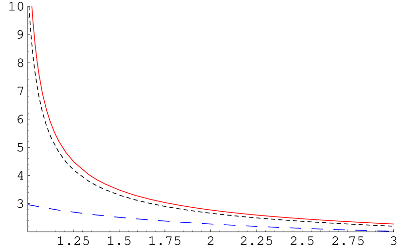
Figure 1: $G^{2}$ at $\mu=0$ for simple (short-dashed line) and HTL QP model as well as the 2-loop perturbative running coupling[11] in $\overline{\hbox{MS}}$ (long-dashed line).

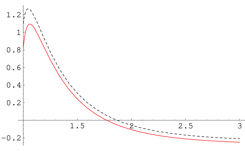
Figure 2: Residual interaction $B/T^{4}$ at $\mu=0$ for HTL- and simple QP model (dashed line).

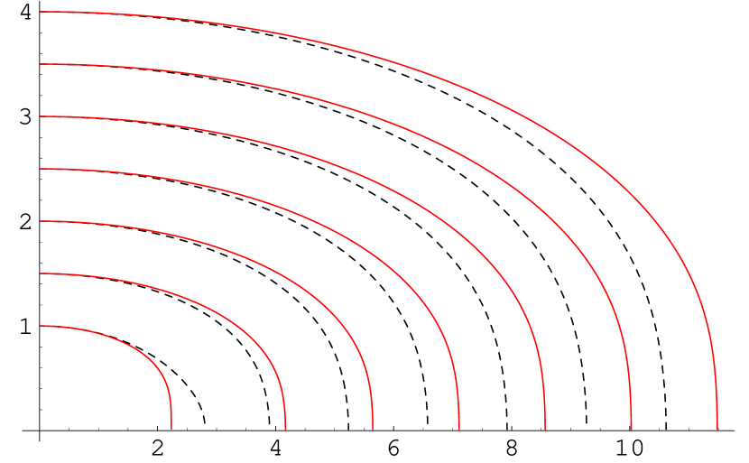
Figure 3: Comparison of the shape of the characteristics (dashed lines indicate those of the simple QP model).

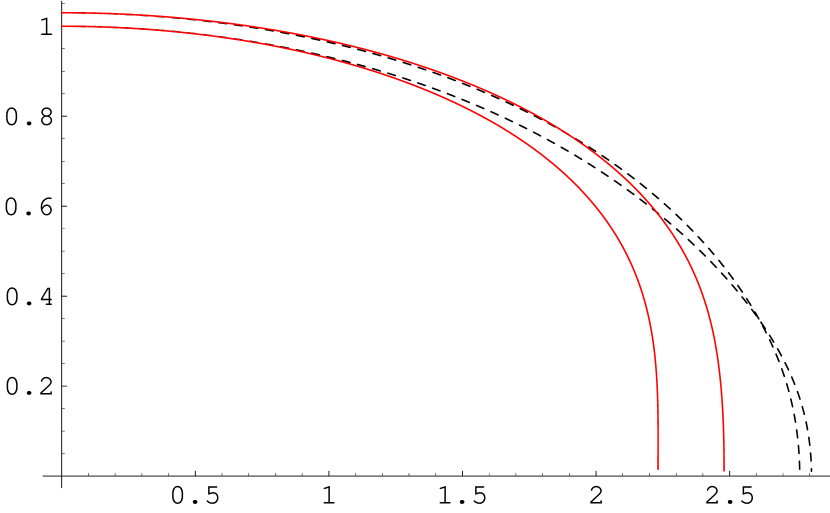
Figure 4: Characteristics starting very near $T_{c}$: HTL- and simple QP model (dashed lines).

While the numerical values of the coefficients $a_{\mu}$ and $a_{T}$ in (2) are approximately equal in the two models, the coefficient $b$ turns out to differ noticeably. This difference is reflected in the shape of the characteristics (figure 4). Interestingly enough, for characteristics of the simple QP model starting very near $T_{c}$ intersections occur[6], while for the HTL model this is not the case (see figure 4).

Integrating the function $B$ along the characteristics (3) and adding the QP contributions one obtains the pressure in the whole $T,\mu$-plane. The result for $T=0$ is shown in figure 6, where the two curves are simple fits to the numerical results[13]. Calculating also the energy density ${\mathcal{E}}$ for $T=0$ one finds that the EOS ${\mathcal{E}}(P)$ for the HTL-model is nearly the same as for the simple model[7]. Finally, a comparison between the QP model characteristics (which are nearly isobars for small $\mu$) starting at $T=T_{c}\equiv\left.T_{c}\right|_{\mu=0}$ and recent lattice data for the phase transition line[4, 5] is shown in figure 6; the curvature of the slope for the QP model characteristics, $T_{c}dT/d\mu^{2}\sim-0.07$ coincides with the central value obtained from one lattice study[5].

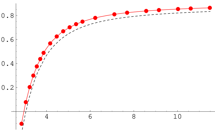
Figure 5: The pressure as a function of $\mu$ at $T=0$ (dashed line corresponds to the simple QP model).

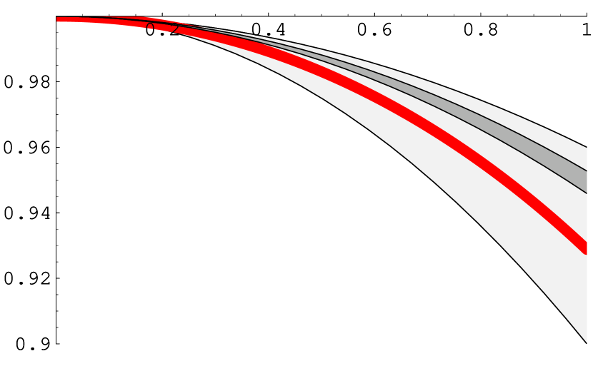
Figure 6: Comparison of the QP model characteristics (thick line) to recent lattice results for the phase transition (light[5] and dark[4] gray region).

5 Conclusions and Outlook

We have investigated the difference between a simple and an HTL QP model at finite chemical potential: although the latter incorporates only slightly more of the plasmon term, there are considerable differences in the characteristics of the flow equation that eliminate the ambiguities of the solutions for the simple QP model[6]. The differences for the thermodynamical quantities are small (even for large $\mu$), which seems to reflect the fact that these are protected by the principle of stationarity. However, they should indicate the trend that an inclusion of the full plasmon term will give. It is encouraging that a first comparison of the QP models and recent lattice results for finite $\mu\lesssim T$ shows some agreement (more extensive studies are in progress).

References

- [1] B. Freedman and L. D. McLerran, Phys. Rev. D17, 1109 (1978); V. Baluni, Phys. Rev. D17, 2092 (1978).
- [2] P. Arnold and C.-x. Zhai, Phys. Rev. D51, 1906 (1995); C.-x. Zhai and B. Kastening, Phys. Rev. D52, 7232 (1995); E. Braaten and A. Nieto, Phys. Rev. D53, 3421 (1996).
- [3] Z. Fodor and S. D. Katz, Phys. Lett. B534, 87 (2002); Z. Fodor, S. D. Katz and K. K. Szabo, hep-lat/0208078 (2002).
- [4] P. de Forcrand and O. Philipsen, Nucl. Phys. B642, 290 (2002).
- [5] C. R. Allton et al., Phys. Rev. D66, 074507 (2002).
- [6] A. Peshier, B. Kämpfer and G. Soff, Phys. Rev. C61, 045203 (2000).
- [7] A. Peshier, B. Kampfer and G. Soff, Phys. Rev. D66, 094003 (2002).
- [8] E. S. Fraga, R. D. Pisarski and J. Schaffner-Bielich, Nucl. Phys. A702, 217 (2002).
- [9] J. O. Andersen and M. Strickland, Phys. Rev. D66, 105001 (2002).
- [10] J. P. Blaizot, E. Iancu and A. Rebhan, Phys. Lett. B470, 181 (1999).
- [11] J. P. Blaizot, E. Iancu and A. Rebhan, Phys. Rev. D63, 065003 (2001).
- [12] A. Ali Khan et al., Phys. Rev. D64, 074510 (2001).
- [13] data file available at http://hep.itp.tuwien.ac.at/~paulrom/.