Analytic Approaches to Kaon Physics

Abstract

Most of the analytic approaches which are used at present to understand the low energy hadronic interactions in Particle Physics, get their inspiration from QCD in the limit of a large number of colors $N_{c}$. I first illustrate this with the example of the left–right correlation function which is an excellent theoretical laboratory. Next, I present the list of observables which have been computed using a large–$N_{c}$ QCD approach. Finally, I discuss in some detail examples which are relevant to lattice QCD, in the sense that we can make comparisons.

1 INTRODUCTION

In the Standard Model, the electroweak interactions of hadrons at very low energies are conveniently described by an effective chiral Lagrangian, which has as active degrees of freedom the low lying $SU(3)$ octet of pseudoscalar particles, plus leptons and photons. The underlying theory is a $SU(3)_{C}\times SU(2)_{L}\times U(1)_{W}$ gauge theory which is formulated in terms of quarks, gluons and leptons, together with the massive gauge fields of the electroweak interactions and the hitherto unobserved Higgs particle. Going from the underlying Lagrangian to the effective chiral Lagrangian is a typical renormalization group problem. It has been possible to integrate the heavy degrees of freedom of the underlying theory, in the presence of the strong interactions, perturbatively, thanks to the asymptotic freedom property of the $SU(3)$–QCD sector of the theory. This brings us down to an effective field theory which consists of the QCD Lagrangian with the $u$, $d$, $s$ quarks still active, plus a string of four quark operators and mixed quark–lepton operators, modulated by coefficients which are functions of the masses of the fields which have been integrated out and the scale $\mu$ of whatever renormalization scheme has been used to carry out this integration. We are still left with the evolution from this effective field theory, appropriate at intermediate scales of the order of a few GeV, down to an effective Lagrangian description in terms of the low–lying pseudoscalar particles which are the Goldstone modes associated with the spontaneous symmetry breaking of chiral–$SU(3)$ in the light quark sector. The dynamical description of this evolution involves genuinely non–perturbative phenomena and it is mostly studied using the techniques of Lattice QCD. In this talk, I shall review the progress which has been made in approaching this last step using analytic methods; in particular when the problem is formulated within the context of QCD in the limit of a large number of colours $N_{c}$.

The suggestion to keep $N_{c}$ in QCD as a free parameter was first made by G. ’t Hooft [1] as a possible way to approach the study of non–perturbative aspects of QCD. The limit $N_{c}\rightarrow\infty$ is taken with the product $\alpha_{\mbox{\rm{\footnotesize s}}}N_{c}$ kept fixed. In spite of the efforts of many illustrious theorists who have worked on the subject, QCD in the large–$N_{c}$ limit ($\mbox{\rm{\footnotesize QCD}}_{\infty}$) still remains unsolved; but many interesting properties have been proved, which suggest that, indeed, the theory in this limit has the bulk of the non–perturbative behaviour of full QCD. In particular, it has been shown that, if confinement persists in this limit, there is spontaneous chiral symmetry breaking [2]. It should be stressed that $\mbox{\rm{\footnotesize QCD}}_{\infty}$ is not just a “wild extrapolation” from $N_{c}=3$ to $N_{c}=\infty$. In fact, $N_{c}$ is really used as a label to select specific topologies among Feynman diagrams. The topology which corresponds to the highest power in the $N_{c}$–label is the one which selects planar diagrams only; and the claim is that this class provides already a good approximation to the full theory.

The spectrum of $\mbox{\rm{\footnotesize QCD}}_{\infty}$ consists of an infinite number of narrow stable meson states which are flavour nonets [3]. This spectrum looks a priori rather different to the one in the real world: the examples of the vector and axial–vector spectral functions measured in $e^{+}e^{-}\rightarrow$ hadrons and in the hadronic $\tau$–decay which are shown below, have indeed a richer structure than just a sum of narrow states. There are, however, many instances where one can show that the observables one is interested in, are given by smooth integrals of specific hadronic spectral functions, though unfortunately in most cases, the specific hadronic spectral functions in question are not accessible from experiments. Typical examples of such observables, are the coupling constants of the effective chiral Lagrangian of QCD at low energies, as well as the coupling constants of the effective chiral Lagrangian of the electroweak interactions of pseudoscalar particles in the Standard Model. What is needed for the evaluation of these coupling constants is not so much the detailed point–by–point knowledge of the relevant hadronic spectrum, but rather a good approximation consistent with the asymptotic properties of QCD, both at short– and long–distances. It is in this sense that the simple $\mbox{\rm{\footnotesize QCD}}_{\infty}$–spectrum becomes useful. It provides a simple parameterization of the physical hadronic spectrum, based on first principles.

2 THE CHIRAL LAGRANGIAN

The strong and electroweak interactions of the Goldstone modes at very low energies are described by an effective Lagrangian which has terms with an increasing number of derivatives (and quark masses if explicit chiral symmetry breaking is taken into account.) Typical terms of the chiral Lagrangian are

$${\cal L}_{\mbox{\rm eff}} = \underbrace{\frac{1}{4}F_{0}^{2}\ \mbox{\rm tr}\left(D_{\mu}UD^{\mu}U^{\dagger}\right)}_{\pi\pi\rightarrow\pi\pi\,,\quad K\rightarrow\pi e\nu}$$ (3)

$$+\underbrace{L_{10}\mbox{\rm tr}\left(U^{\dagger}F_{R\mu\nu}UF_{L}^{\mu\nu}\right)}_{\pi\rightarrow e\nu\gamma}+\cdots$$

$$+\underbrace{e^{2}C\mbox{\rm tr}\left(Q_{R}UQ_{L}U^{\dagger}\right)}_{-e^{2}C\frac{2}{F_{0}^{2}}\left(\pi^{+}\pi^{-}+K^{+}K^{-}\right)}+\cdots$$

$$-\underbrace{\frac{G_{\mbox{\rm{\small F}}}}{\sqrt{2}}V_{ud}V^{*}_{us}\ g_{\underline{8}}F_{0}^{4}\left(D_{\mu}UD^{\mu}U^{\dagger}\right)_{23}}_{{K\rightarrow\pi\pi\,,\quad K\rightarrow\pi\pi\pi}}+\cdots\,,$$ (4)

where $U$ is a $3\times 3$ unitary matrix in flavour space which collects the Goldstone fields and which under chiral rotations transforms as $U\rightarrow V_{R}UV_{L}^{\dagger}$; $D_{\mu}U$ denotes the covariant derivative in the presence of external vector and axial–vector sources. The first line is the lowest order term in the sector of the strong interactions [4], $F_{0}$ is the pion–decay coupling constant in the chiral limit where the light quark masses $u$, $d$, $s$ are neglected ($F_{0}\simeq 90~{}\mbox{\rm MeV}$); the second line shows one of the couplings at ${\cal O}(p^{4})$ [5, 6]; the third line shows the lowest order term which appears when photons and $Z^{\prime}s$ are integrated out ($Q_{L}=Q_{R}=\mbox{\rm diag.}[(2/3,-1/3,-1/3]$), in the presence of the strong interactions ; the fourth line shows one of the lowest order terms in the sector of the weak interactions. The typical physical processes to which each term contributes are indicated under the braces. Each term is modulated by a coupling constant: $F_{0}^{2}$, $L_{10}$,… $C$…$g_{\underline{8}}$…, which encodes the underlying dynamics responsible for the appearance of the corresponding effective term. The evaluation of these couplings from the underlying theory is the question we are interested in. The coupling $g_{\underline{8}}$ for example, governs the strength of the dominant $\Delta I=1/2$ transitions for $K$–decays to leading order in the chiral expansion.

2.1 Two crucial observations

There are two crucial observations to be made concerning the relation of these low energy constants to the underlying theory.

i) The low–energy constants of the Strong Lagrangian, like $F_{0}^{2}$ and $L_{10}$, are the coefficients of the Taylor expansion of appropriate QCD Green’s Functions. For example, with $\Pi_{LR}(Q^{2})$ the correlation function of a left–current with a right–current in the chiral limit:

$$\int\!d^{4}x\ e^{iq\cdot x}\langle 0|T\!\left(\bar{u}_{L}\gamma^{\mu}d_{L}(x)\bar{u}_{R}\gamma^{\nu}d_{R}(0)^{\dagger}\right)|0\rangle$$

$$=\frac{1}{2i}(q^{\mu}q^{\nu}-g^{\mu\nu}q^{2})\Pi_{LR}(Q^{2})\,,$$ (5)

the Taylor expansion

$$-Q^{2}\Pi_{LR}(Q^{2})|_{Q^{2}\rightarrow 0}=F_{0}^{2}-4L_{10}\ Q^{2}\!+\cdots\,,$$ (6)

defines the constants $F_{0}^{2}$ and $L_{10}$.

ii) By contrast, the low–energy constants of the Electroweak Lagrangian, like e.g. $C$ and $g_{8}$, are integrals of appropriate QCD Green’s Functions. For example [7],

$$C\!=\!\frac{3}{32\pi^{2}}\int_{0}^{\infty}\!dQ^{2}\frac{M_{Z}^{2}}{Q^{2}+M_{Z}^{2}}\left(-Q^{2}\Pi_{LR}(Q^{2})\right)\,.$$ (7)

Their evaluation appears to be, a priori, quite a formidable task because they require the knowledge of Green’s functions at all values of the euclidean momenta; i.e. they require a precise matching of the short–distance and the long–distance contributions to the underlying Green’s functions.

These two observations are generic in the case of the Standard Model, independently of the $1/N_{c}$–expansion. The large–$N_{c}$ approximation helps, however, because it restricts the analytic structure of the Green’s functions in general, and $\Pi_{LR}(Q^{2})$ in particular, to be meromorphic functions: they only have poles as singularities; e.g., in $\mbox{\rm{\footnotesize QCD}}_{\infty}$,

$$\Pi_{LR}(Q^{2})\!=\!\!\sum_{V}\!\frac{f_{V}^{2}M_{V}^{2}}{Q^{2}+M_{V}^{2}}-\!\sum_{A}\!\frac{f_{A}^{2}M_{A}^{2}}{Q^{2}+M_{A}^{2}}\!-\!\frac{F_{0}^{2}}{Q^{2}}\!\,,$$ (8)

where the sums are extended to an infinite number of states. In practice, however, in the case of Green’s functions which are order parameters of spontaneous chiral symmetry breaking (like $\Pi_{LR}$ in the chiral limit), these sums will be restricted to a finite number of states.

2.2 Sum Rules

There are two types of important restrictions on Green’s functions like $\Pi_{LR}(Q^{2})$. One type follows from the fact that, as already stated above, the Taylor expansion at low euclidean momenta must match the low energy constants of the strong chiral Lagrangian. This results in a series of long–distance sum rules like e.g.

$$\sum_{V}f_{V}^{2}-\sum_{A}f_{A}^{2}=-4L_{10}\,.$$ (9)

Another type of constraints follows from the short–distance properties of the underlying Green’s functions. The behaviour at large euclidean momenta of the Green’s functions which govern the low energy constants of the chiral Lagrangian can be obtained from the operator product expansion (OPE) of local currents in QCD. In the large–$N_{c}$ limit, this results in a series of algebraic sum rules [8] which restrict the coupling constants and masses of the hadronic poles. In the case of the $LR$–correlation function in Eq. (8) one has e.g.,

$$\sum f_{V}^{2}M_{V}^{2}-\sum f_{A}^{2}M_{A}^{2}-F_{0}^{2}=0\,,$$ (10)

$$\sum f_{V}^{2}M_{V}^{4}-\sum f_{A}^{2}M_{A}^{4}=0\,,$$ (11)

$$\sum f_{V}^{2}M_{V}^{6}-\sum f_{A}^{2}M_{A}^{6}\simeq-4\pi\alpha_{s}\langle\bar{\psi}\psi\rangle^{2}\,.$$ (12)

The sum rules in Eqs. (10) and (11) are the celebrated Weinberg sum rules, which follow from the fact that in the chiral limit, there are no ${\cal O}(1/Q^{2})$ terms and no ${\cal O}(1/Q^{4})$ terms in the OPE of $\Pi_{LR}(Q^{2})$. The third sum rule in Eq. (12) [8], follows from the matching between the ${\cal O}(1/Q^{6})$–terms in the $\mbox{\rm{\footnotesize QCD}}_{\infty}$ expression in Eq. (8) and the corresponding one in the OPE (evaluated at leading ${\cal O}(\alpha_{\mbox{\rm{\scriptsize s}}}N_{c}^{2})$ [9]). In principle there are an infinite number of sum rules in $\mbox{\rm{\footnotesize QCD}}_{\infty}$ which relate the masses and couplings of the $\mbox{\rm{\footnotesize QCD}}_{\infty}$ narrow states to the local order parameters which appear in the OPE and to the non–local order parameters which govern the chiral expansion in the strong sector.

3 THE $\pi^{+}-\pi^{0}$ MASS DIFFERENCE AS A THEORETICAL LABORATORY

The physical effect of the coupling $C$ in Eq. (3) is to give a mass, mostly of electromagnetic origin, to the charged pions:

$$m_{\pi^{\pm}}^{2}\big{|}_{\mbox{\rm{\tiny EM}}}=\frac{\alpha}{\pi}\frac{3}{4F_{0}^{2}}\int_{0}^{\infty}dQ^{2}\left[-Q^{2}\Pi_{LR}(Q^{2})\right]\,.$$ (13)

The first evaluation of this integral was done by F. Low and collaborators in 1967  [10]. What I am going to do next is, simply, to put their phenomenological calculation within the context of $\mbox{\rm{\footnotesize QCD}}_{\infty}$.

As already stated, the function $\Pi_{LR}(Q^{2})$ in $\mbox{\rm{\footnotesize QCD}}_{\infty}$ is a meromorphic function. That means that within a finite radius in the complex $Q^{2}$–plane it only has a finite number of poles. The natural question which arises is: what is the minimal number of poles required to satisfy the OPE constraints? The answer to that follows from a well known theorem in analysis [11], which when applied to our case, states that the function

$$-Q^{2}\Pi_{LR}(Q^{2})\equiv\Delta[z]\quad\mbox{\rm with}\quad z=\frac{Q^{2}}{M_{V}^{2}}\,,$$ (14)

and $M_{V}$ the mass of the lowest narrow state, has the property that

$${\cal N}-{\cal P}=\frac{1}{2\pi i}\oint\frac{\Delta^{\prime}[z]}{\Delta[z]}dz\,,$$ (15)

where ${\cal N}$ is the number of zeros and ${\cal P}$ is the number of poles inside the integration contour in the complex $z$–plane (a zero and/or a pole of order m is counted m times.) For a circle of radius sufficiently large, we simply have that ${\cal N}-{\cal P}=-p\,,$ where $p$ denotes the asymptotic power fall–off in $1/z$ of the $\Delta[z]$ function. Identifying the power $p$ with the leading power predicted by the OPE, and from the fact that ${\cal N}\geq 0$, there follows that ${\cal P}\geq p_{\mbox{\rm{\tiny OPE}}}$. In our case $p_{\mbox{\rm{\tiny OPE}}}=2\Rightarrow{\cal P}\geq 2$ and the minimal hadronic approximation (MHA) compatible with the OPE requires two poles : one vector state and one axial–vector state. The MHA to the $\mbox{\rm{\footnotesize QCD}}_{\infty}$ expression in Eq. (8) is then the simple function

$$-Q^{2}\Pi_{LR}(Q^{2})=F_{0}^{2}\frac{M_{V}^{2}M_{A}^{2}}{(Q^{2}+M_{V}^{2})(Q^{2}+M_{A}^{2})}\,.$$ (16)

Inserting this function in Eq. (13) gives a prediction for the electromagnetic $\pi^{+}-\pi^{0}\equiv\Delta m_{\pi}$ mass difference, with the result 

$$\Delta m_{\pi}=(4.9\pm 0.4)\,\mbox{\rm MeV}\,,$$ (17)

to be compared with the experimental value [14]

$$\Delta m_{\pi}=(4.5936\pm 0.0005)\,\mbox{\rm MeV}\,.$$ (18)

3.1 The real world and the MHA to $\mbox{\rm{\footnotesize QCD}}_{\infty}$

The spectral function of the correlation function defined in Eq. (2.1) can be obtained from measurements of the hadronic $\tau$–decay spectrum (vector–like decays minus axial–vector like decays). We plot in Figure 1 the experimental determination of $\frac{1}{\pi}\mbox{\rm Im}\Pi_{LR}(t)$, obtained from the ALEPH collaboration data [15], versus the invariant hadronic mass squared $t$ in the accessible region $0\leq t\leq m_{\tau}^{2}$.

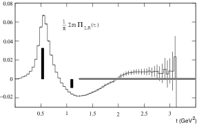
Figure 1: The Spectral Function $\frac{1}{\pi}\mbox{\rm Im}\Pi_{LR}(t)$, obtained from the ALEPH data [15] compared to the MHA to $\mbox{\rm{\footnotesize QCD}}_{\infty}$.

In this case, the corresponding spectrum of the MHA to $\mbox{\rm{\footnotesize QCD}}_{\infty}$ consists of the pion pole (not shown in the figure), a vector narrow state(the $\rho$) and an axial–vector narrow state (the $A_{1}$). At this level of approximation, and in the chiral limit, the rest of the vector and axial–vector states are taken to be degenerate and cancel in the difference, a fact which is simulated by the horizontal continuum line in the figure. Looking at this plot, one can hardly claim that this approximation reproduces the details of the experimental data. However, with $\Pi_{LR}(Q^{2})$ determined from the spectral function by the unsubtracted dispersion relation

$$\Pi_{LR}(Q^{2})=\int_{0}^{\infty}dt\frac{1}{t+Q^{2}}\frac{1}{\pi}\mbox{\rm Im}\Pi_{LR}(t)\,,$$ (19)

the corresponding plot of the function $\frac{-Q^{2}}{F_{0}^{2}}\Pi_{LR}(Q^{2})$ versus the euclidean variable $Q^{2}=-t$ is shown in Fig 2. The solid curve is the one corresponding to the simple MHA in Eq. (16) and the dotted curve the one from the experimental data in Fig 1. One can see that, by contrast to what happens in the Minkowski region shown in Fig. 1, the corresponding curves in the euclidean region are both very smooth and in fact the MHA already provides a rather good interpolation between the asymptotic regimes where, by construction, it has been constrained to satisfy the lowest order chiral behaviour in Eq. (6), and the two Weinberg sum rules: the OPE constraints in Eqs. (10) and (11). This good interpolation is the reason why the integral in Eq. (7), evaluated at the MHA, already reproduces the experimental result rather well .

3.2 Other Analytic Approaches

At this stage, it is illustrative to compare the large–$N_{c}$ approach we have discussed so far with other analytic approaches in the literature. The $\Pi_{LR}$ correlation function provides us with an excellent theoretical laboratory to do this comparison. The different shapes of $\frac{-Q^{2}}{F_{0}^{2}}\Pi_{LR}(Q^{2})$ predicted by other analytic approaches are collected in Fig. 2. Here, several comments are in order.

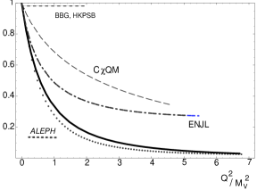
Figure 2: Plot of $\frac{-Q^{2}}{F_{0}^{2}}\Pi_{LR}(Q^{2})$ in the euclidean region. The solid curve is the one corresponding to the simple MHA in Eq. (16) and the dotted curve the one from the experimental data in Fig 1. The other curves are the predictions of various models discussed in the text.

a) The suggestion to use a large–$N_{c}$ QCD framework combined with $\chi$PT cut–off loops, was first proposed by Bardeen, Buras and Gérard in a series of seminal papers [16, 17, 18]. The same method has been applied by the Dortmund group [19], in particular to the evaluation of $\epsilon^{\prime}/\epsilon$. In this approach the hadronic ansatz to the Green’s functions consists of Goldstone poles alone and, therefore, integrals like the one in Eq. (7) become UV–divergent (often quadratically divergent) since the correct QCD short–distance behaviour is not implemented. In practice the integrals are cut at a physical cut off: $\Lambda\sim 1~{}\mbox{\rm GeV}$. In the case we are considering, the predicted shape of the LR–correlation function normalized to its value at $Q^{2}=0$ is a constant all the way up to the chosen cut–off value, as shown by the BBG, HKPSB line (the horizontal dotted line) in Fig. 2.

b) The Trieste group evaluate the relevant Green’s functions using the constituent chiral quark model (C$\chi$QM) proposed in refs. [20] and [21, 22]. They have obtained a long list of predictions [23], in particular $\epsilon^{\prime}/\epsilon$. The model gives an educated first guess of the low–$Q^{2}$ behaviour of the Green’s functions, as one can judge from the C$\chi$QM–curve (dashed curve) in Fig. 2, but it fails to reproduce the short–distance QCD–behaviour. Another objection to this approach is that the “natural matching scale” to the short–distance behaviour in this model should be $\sim 4M_{Q}^{2}$ ($M_{Q}$ the constituent quark mass), which is too low to be trusted.

c) The extended Nambu–Jona-Lasinio (ENJL) model was developed as an improvement on the C$\chi$QM, since in a certain way it incorporates the vector–like fluctuations of the underlying QCD theory which are known to be phenomenologically important (see e.g. refs. [24, 25] where other references can also be found). The model is rather successful in predicting the low–energy $O(p^{4})$ constants of the chiral Lagrangian [24]. It has, indeed, a better low–energy behaviour than the C$\chi$QM, as the ENJL–curve (dot–dashed) in Fig. 2 shows; but it fails to reproduce the short–distance behaviour of the OPE in QCD. Arguments, however, to do the matching to short–distance QCD have been forcefully elaborated in refs. [26], which also give a lot of numerical predictions; a large value for $\epsilon^{\prime}/\epsilon$ in particular.

The problem with the ENJL model as a plausible model of large–$N_{c}$ QCD, is that the on–shell production of unconfined constituent quark $Q\bar{Q}$ pairs that it predicts, violates the large–$N_{c}$ QCD counting rules. In fact, as shown in ref. [12], when the unconfining pieces in the ENJL spectral functions are removed by adding an appropriate series of local counterterms, the resulting theory is entirely equivalent to an effective chiral meson theory with three narrow states V, A and S; very similar to the phenomenological Resonance Chiral Lagrangians proposed in refs. [27, 28]. These Lagrangians can be viewed, therefore, as particular models of large–$N_{c}$ QCD. They predict the same Green’s functions as the MHA to $\mbox{\rm{\footnotesize QCD}}_{\infty}$ discussed above, in some particular cases but not in general (see e.g. the three–point functions discussed in ref. [29]).

In view of the difficulties which the analytic approaches discussed in a), b) and c) above, have in reproducing the shape of the simplest Green’s function one can think of, it is difficult to attribute more than a qualitative significance to their “predictions”; $\epsilon^{\prime}/\epsilon$ in particular, which requires the interplay of several other Green’s functions much more complex than $\Pi_{LR}(Q^{2})$.

4 METHODOLOGY, APPLICATIONS

The $\mbox{\rm{\footnotesize QCD}}_{\infty}$ approach that we are proposing in order to compute a specific coupling of the chiral electroweak Lagrangian consists of the following steps:

1. Identify the relevant Green’s functions.

   In most cases of interest, the underlying QCD Green’s functions in question are two–point functions with additional zero momentum insertions of vector, axial vector, scalar and pseudoscalar currents. The higher the power in the chiral expansion, the higher will be the number of zero momentum insertions. This step is totally general and does not invoke any large–$N_{c}$ approximation.

2. Work out the short–distance behaviour and the long–distance behaviour of the relevant Green’s functions.

   The long–distance behaviour is governed by the Goldstone singularities and can be obtained from $\chi$PT. The short–distance behaviour is governed by the OPE of the currents through which the hard momenta flows. Again, this step is well defined independently of the large–$N_{c}$ expansion; in practice, however, the calculations simplify when restricted to the appropriate order in the $1/N_{c}$–expansion one is interested in. In particular, chiral loops are subleading in the $1/N_{c}$–expansion.

3. Introduce a large–$N_{c}$ approximation for the underlying Green’s functions.

   As already mentioned, Green’s functions in $\mbox{\rm{\footnotesize QCD}}_{\infty}$ are meromorphic functions. The minimal hadronic approximation (MHA) that we are proposing consists in limiting the number of poles to the minimum required to satisfy the leading power fall–off at short–distances, as well as the appropriate $\chi$PT long–distance constraints.

The three steps above can be done analytically, which helps to unravel the intricacies of the underlying dynamics. The method is, in principle, improvable (unlike the other models discussed above). It can be improved by adding more constraints from the next–to–leading short–distance inverse power behaviour in the OPE and/or higher orders in the chiral expansion. This has been tested within a toy model of $QCD_{\infty}$ in ref. [30]

We have checked this approach with the calculation of a few low–energy observables:

i) The electroweak $\Delta m_{\pi}$ mass difference which we have already discussed [7].

ii) The hadronic vacuum polarization contribution to the anomalous magnetic moment of the muon $a_{\mu}$. The MHA in this case requires one vector–state pole and a perturbative QCD continuum. The absence of dimension two operators in QCD in the chiral limit, constrains the threshold of the continuum. The result thus obtained [31] is compatible with the more precise phenomenological determinations which use experimental input.

iii) The $\pi^{0}\rightarrow e^{+}e^{-}$ and $\eta\rightarrow\mu^{+}\mu^{-}$ decay rates. These processes are governed by a $\langle PVV\rangle$ three–point function, with the $Q^{2}$–momentum flowing through the two $V$–currents. The MHA in this case requires a vector–pole and a double vector–pole. The predictions [33] of the branching ratios $\frac{\Gamma(P\rightarrow l^{+}l^{-})}{\Gamma(P\rightarrow\gamma\gamma)}$ are in good agreement with the present experimental determinations.

These successful predictions have encouraged some of us to pursue a systematic analysis of $K$–physics observables within the same large–$N_{c}$ framework. So far, the following calculations have been made:

• The $B_{K}$–Factor in the Chiral Limit [34].

• Weak Matrix Elements of the Electroweak Penguin Operators $Q_{7}$ and $Q_{8}$ [32, 35].

• Hadronic Light–by–Light Scattering Contribution to the Muon $g-2$ [36, 37].

• Electroweak Hadronic Contributions to the Muon $g-2$ [38].

We also have preliminary results on:

• The Long–Distance Contribution to the $K_{L}\rightarrow\mu^{+}\mu^{-}$ Decay Rate [39].

• Weak Matrix Elements of the Strong Penguin Operators $Q_{4}$ and $Q_{6}$ [40].

5 FACTOR $B_{K}$ OF $K^{0}-\bar{K}^{0}$ MIXING

The factor in question is conventionally defined by the matrix element of the four–quark operator $Q_{\Delta S=2}(x)=(\bar{s}_{L}\gamma^{\mu}d_{L})(\bar{s}_{L}\gamma_{\mu}d_{L})(x)$:

$$\langle\bar{K}^{0}|Q_{\Delta S=2}(0)|K^{0}\rangle=\frac{4}{3}f_{K}^{2}M_{K}^{2}B_{K}(\mu)\,.$$ (20)

To lowest order in the chiral expansion the operator $Q_{\Delta S=2}(x)$ bosonizes into an $O(p^{2})$ term:

$$-\frac{F_{0}^{4}}{4}g_{\Delta S=2}(\mu)\underbrace{\left[(D^{\mu}U^{\dagger})U\right]_{23}\left[(D_{\mu}U^{\dagger})U\right]_{23}}_{\frac{2}{F_{0}^{2}}\partial^{\mu}K^{0}\partial_{\mu}K^{0}-(r^{\mu})_{23}(r_{\mu})_{23}+\cdots}\,,$$ (21)

with $g_{\Delta S=2}(\mu)$ the low energy constant (which depends on the renormalization scale $\mu$) to be determined. A convenient choice of the underlying Green’s function here is the four–point function $W_{LRLR}^{\mu\alpha\nu\beta}(q,l)$ of two left–currents $(\bar{s}_{L}\gamma^{\mu}d_{L})$ and $(\bar{s}_{L}\gamma^{\nu}d_{L})$, which carry the $q$–momentum one has to integrate over, and two right–currents $(\bar{d}_{R}\gamma^{\alpha}s_{R})$ and $(\bar{d}_{R}\gamma^{\beta}s_{R})$ with soft $l$–momentum insertions, which couple to the external $(r_{\alpha})_{32}$– and $(r_{\beta})_{32}$–sources. The coupling constant $g_{\Delta S=2}(\mu)$, which has to be evaluated in the same renormalization scheme as the Wilson coefficient $C_{\Delta S=2}(\mu)$ has been evaluated, is then given by the integral [34]

$$g_{\Delta S=2}(\mu)\!=\!1-\frac{1}{32\pi^{2}F_{0}^{2}}\!\left[\frac{\left(4\pi\mu^{2}\right)^{\epsilon/2}}{\Gamma(2-\epsilon/2)}\!\int_{0}^{\infty}\!\!\!\frac{dQ^{2}}{(Q^{2})^{\epsilon/2}}\times\right.$$

$$\left.\underbrace{\left(\frac{-g_{\alpha\beta}}{3}\right)\!\!\int\!d\Omega_{q}\lim_{l\rightarrow 0}g_{\mu\nu}W_{LRLR}^{\mu\alpha\nu\beta}(q,l)}_{W_{LL}(Q^{2})}\right]_{\overline{MS}}\!\!\,,$$ (22)

conceptually similar to the one which determines the electroweak constant $C$ in Eq. (7). The renormalization–scale invariant $\hat{B}_{K}$–factor is then given by the product

$$\hat{B}_{K}=\frac{3}{4}C_{\Delta S=2}(\mu)\times g_{\Delta S=2}(\mu)\,.$$ (23)

The large–$N_{c}$ hadronic approximation of the Green’s function $W_{LL}(Q^{2})$ in Eq. (22), which fulfills the leading OPE short–distance constraint and the long–distance constraints which fix $W_{LL}(0)$ and $W_{LL}^{`}(0)$ in $\chi$PT, requires one vector–pole, a double vector–pole and a triple vector–pole  The integral in Eq. (22) can then be evaluated, with the result [34]

$$\hat{B}_{K}=0.38\pm 0.11\,.$$ (24)

The $\mu$–scale and renormalization scheme dependence in $g_{\Delta S=2}(\mu)$ cancels with the one in $C_{\Delta S=2}(\mu)$, when evaluated at the same approximation in the $I/N_{c}$–expansion.

When comparing this result to other determinations, specially in Lattice QCD, it should be realized that the unfactorized contribution in Eq. (22) is the one in the chiral limit. It is possible, in principle, to calculate chiral corrections within the same large–$N_{c}$ approach, but this has not yet been done.

The result in Eq. (24) is compatible with the old current algebra prediction [41] which, to lowest order in $\chi$PT, relates the $B_{K}$–factor to the $K^{+}\rightarrow\pi^{+}\pi^{0}$ decay rate. In fact, our calculation can be viewed as a successful prediction of the $K^{+}\rightarrow\pi^{+}\pi^{0}$ decay rate !

As discussed in ref. [42], the bosonization of the four–quark operator $Q_{\Delta S=2}$ and the bosonization of the operator $Q_{2}-Q_{1}$ which generates $\Delta I=1/2$ transitions, are related to each other in the combined chiral limit and next–to–leading order in the $1/N_{c}$–expansion, when mixing with the penguin operators is neglected. Lowering the value of $\hat{B}_{K}$ from the factorized ${\cal O}(N_{c}^{2})$ prediction: $\hat{B}_{K}=3/4$, to the result in Eq. (24), is correlated with an increase of the coupling constant $g_{\underline{8}}$ in the lowest order effective chiral Lagrangian (see Eq. (4)) which generates $\Delta I=1/2$ transitions, and provides a first step towards a quantitative understanding of underlying dynamics of the $\Delta I=1/2$ rule.

6 ELECTROWEAK PENGUINS

We shall be next concerned with the four–quark operators generated by the so called electroweak penguin diagrams of the Electroweak Theory

$${\cal L}\Rightarrow\cdots C_{7}(\mu)Q_{7}+C_{8}(\mu)Q_{8}\,,$$ (25)

with $C_{7}(\mu)$, $C_{8}(\mu)$ the Wilson coefficients of the operators

$$Q_{7}=6(\bar{s}_{L}\gamma^{\mu}d_{L})\sum_{q=u,d,s}e_{q}(\bar{q}_{R}\gamma_{\mu}q_{R})\,,$$ (26)

$$Q_{8}=-12\sum_{q=u,d,s}e_{q}(\bar{s}_{L}q_{R})(\bar{q}_{R}d_{L})\,.$$ (27)

These operators generate terms of $O(p^{0})$ in the effective chiral Lagrangian[43]; therefore, their matrix elements, although suppressed by an $e^{2}$ factor, are chirally enhanced. Furthermore, the Wilson coefficient $C_{8}$ has a large imaginary part induced by the top–quark integration, which makes the matrix elements of the $Q_{8}$ operator to be particularly important in the evaluation of $\epsilon^{\prime}/\epsilon$.

Within the large–$N_{c}$ framework, the bosonization of these operators produce matrix elements with the following counting

$$\langle Q_{7}\rangle|_{O(p^{0})}=\underline{O(N_{c})}+O(N_{c}^{0})\,,$$ (28)

$$\langle Q_{8}\rangle|_{O(p^{0})}=\underline{O(N_{c}^{2})}+\!\!\!\!\!\!\!\!\!\underbrace{O(N_{c}^{0})}_{{\mbox{\rm Zweig suppressed}}}\,.$$ (29)

6.1 Bosonization of $Q_{7}$

The bosonization of the $Q_{7}$ operator to $O(p^{0})$ in the chiral expansion and to $O(N_{c})$ is very similar to the calculation of the $Z$–contribution to the coupling constant $C$ in Eq. (7). An evaluation which also takes into account the renormalization scheme dependence has been recently made in ref. [35] with the result:

$$\langle Q_{7}\rangle|_{{\cal O}(p^{0})}=6\ \underbrace{\langle 0|(\bar{s}_{L}\gamma^{\mu}d_{L})(\bar{d}_{R}\gamma_{\mu}s_{R})|0\rangle}_{\langle O_{1}(\mu)\rangle}\times$$

$$\mbox{\rm tr}\left(U\lambda_{L}^{(23)}U^{\dagger}Q_{R}\right)^{{\dagger}}\,,\quad\mbox{\rm and}\quad\lambda_{L}^{(23)}=\delta_{i2}\delta_{j3}\,.$$ (30)

Here, the vev $\langle O_{1}(\mu)\rangle$ is given by the integral

$$\langle O_{1}(\mu)\rangle=\left\{\frac{3(\epsilon-3)}{16\pi^{2}}\frac{(4\pi\mu^{2})^{\,\epsilon/2}}{\Gamma(2-\epsilon/2)}\times\right.$$

$$\int_{0}^{\infty}dQ^{2}\left.(Q^{2})^{1-\epsilon/2}\left(-Q^{2}\Pi_{LR}(Q^{2})\right)\right\}_{\overline{MS}}\,,$$ (31)

with $\Pi_{LR}(Q^{2})$ the same correlation function as in Eq. (2.1). In $\mbox{\rm{\footnotesize QCD}}_{\infty}$ this integral can be, formally, evaluated exactly. When restricted to the same MHA which has been used to calculate $\Delta m_{\pi}$, one gets the simple result

$$\langle O_{1}\rangle=\frac{3}{32\pi^{2}}\!\left[f_{V}^{2}M_{V}^{6}\ln\!\frac{\Lambda^{2}}{M_{V}^{2}}\!-\!f_{A}^{2}M_{A}^{6}\ln\!\frac{\Lambda^{2}}{M_{A}^{2}}\right]\,,$$ (32)

where $\Lambda^{2}\!\!=\!\!\mu^{2}\exp(1/3+\kappa)$, with $\kappa\!\!=\!-1/2$ in the naive dimensional renormalization scheme (NDR) and $\kappa\!\!=\!\!+3/2$ in the ’t Hooft–Veltman scheme (HV).

6.2 Bosonization of $Q_{8}$

To lowest ${\cal O}(p^{0})$ in the chiral expansion, the four–quark operator $Q_{8}$ bosonizes as follows

$$\langle Q_{8}\rangle|_{{\cal O}(p^{0})}\!=\!-12\underbrace{\langle O_{2}(\mu)\rangle}_{\langle 0|(\bar{s}_{L}s_{R})(\bar{d}_{R}d_{L})|0\rangle}\mbox{\rm tr}\left(U\lambda_{L}^{(23)}U^{\dagger}Q_{R}\right)^{{\dagger}}\!\!\,.$$

As noted in refs. [44, 35], the vev $O_{2}(\mu)$ also appears in the Wilson coefficient of the $1/Q^{6}$ term in the OPE of the same $\Pi_{LR}(Q^{2})$ correlation function as in Eq. (2.1), for which the MHA to $\mbox{\rm{\footnotesize QCD}}_{\infty}$ gives a rather good approximation, as we have already discussed. This offers the possibility of obtaining an estimate of the vev $O_{2}(\mu)$ beyond the large–$N_{c}$ approximation, where $O_{2}\!\Rightarrow\!\frac{1}{4}\langle\bar{\psi}\psi\rangle^{2}$, and, therefore, without having to fix a value for the $\langle\bar{\psi}\psi\rangle$–condensate, which is poorly known. Unfortunately, as one can judge from the results in Table 1, different methods to extract the value of $O_{2}(\mu)$ lead, at present, to rather different values for the weak matrix elements:

$$M_{7,8}\equiv\langle(\pi\pi)_{I=2}|Q_{7,8}|0\rangle\,,\quad\mbox{\rm at}\quad\mu=2~{}\mbox{\rm GeV}\,.$$ (33)

In view of the diversity of results obtained with the dispersive approach, depending on which type of sum rules are used; and the unknown systematic errors of the quenched approximation and the chiral limit extrapolations in the lattice results, it looks like it will take some time before one can claim that these matrix elements are known reliably.

Table 1: Matrix Elements Results for $M_{7,8}$ (see Eq. (33)) in $\mbox{\rm GeV}^{3}$ using different methods.

METHOD	$M_{7}$(NDR)	$M_{7}$(HV)	$M_{8}$(NDR)	$M_{8}$(HV)
Large–$N_{c}$ MHA
Knecht, Peris, de Rafael	$0.11\pm 0.03$	$0.67\pm 0.20$	$2.3\pm 0.7$	$2.5\pm 0.8$
(with $\alpha_{\mbox{\rm{\scriptsize s}}}^{2}$ corrects.) [35, 46]
Dispersive Approach
Narison [47]	$0.17\pm 0.05$		$1.4\pm 0.3$
Cirigliano et al [48]	$0.16\pm 0.10$	$0.49\pm 0.07$	$2.2\pm 0.7$	$2.5\pm 0.7$
Bijnens et al [49]	$0.24\pm 0.03$	$0.37\pm 0.08$	$1.2\pm 0.8$	$1.3\pm 0.8$
Cirigliano et al (OPAL data) [50]	$0.21\pm 0.05$		$1.7\pm 0.3$
Lattice QCD
Bhattacharia et al [51]	$(0.32\pm 0.06)$		$(1.2\pm 0.2)$
Donini et al [52]	$0.11\pm 0.04$	$0.18\pm 0.06$	$0.51\pm 0.10$	$0.62\pm 0.12$
RBC coll. [53]	$(0.27\pm 0.03)$		$(1.1\pm 0.2)$
CP-PACS coll [54]	$(0.24\pm 0.03)$		$(1.0\pm 0.2)$

Only the results obtained with methods which can exhibit an explicit dependence on the renormalization scale are quoted in this Table. The numbers in brackets have been obtained after informal private discussions with some of the authors of the various lattice collaboration.

6.3 Test of the Zweig Rule

Besides the important issue of getting an accurate determination of the $Q_{8}$ matrix elements, a reliable determination of the vev $\langle 0|(\bar{s}_{L}s_{R})(\bar{d}_{R}d_{L})|0\rangle$ would be most welcome as a test of the Zweig rule in the scalar and pseudoscalar sectors. More precisely,

$$\langle O_{2}(\mu)\rangle=\frac{1}{4}\langle\bar{\psi}\psi\rangle^{2}+\langle 0|(\bar{s}_{L}s_{R})(\bar{d}_{R}d_{L})|0\rangle_{c}\,,$$ (34)

where the unfactorized contribution (the second term) involves Feynman diagrams which require gluon exchanges between at least two quark loops. These are the so called Zweig–suppressed contributions, which are indeed ${\cal O}(N_{c}^{0})$ in the $1/N_{c}$ expansion. There are reasons to suspect that subleading terms in the $1/N_{c}$ expansion involving Green’s functions of scalar (and pseudoscalar) density operators might be important, unlike those which only involve vector (and axial-vector) currents. There are several phenomenological examples of this: the $\eta^{\prime}$ mass, the possible existence of a broad $\sigma$ meson, large final state interactions in states with $J=0$ and $I=0$, etc. We are considering the possibility that the appropriate expansion for these exceptional Green’s functions could be a $1/N_{c}$ expansion in which $n_{f}/N_{c}$ is held fixed, where $n_{f}$ denotes the number of light flavours; the kind of expansion originally advocated by G. Veneziano [45].

Formally, the connected part of the vev $\langle 0|(\bar{s}_{L}s_{R})(\bar{d}_{R}d_{L})|0\rangle_{c}$ is defined by the integral

$$\frac{1}{i}\left(\int\frac{d^{D}q}{(2\pi)^{D}}\,\Psi_{ds}(Q^{2})\right)_{\overline{\mbox{\rm{\footnotesize MS}}}}^{\mbox{\rm\tiny ren.}}\,,$$ (35)

with $\Psi_{ij}(Q^{2})$ the two–point function

$$\frac{i}{4}\int d^{4}xe^{iq.x}\left\{\langle 0|T\left[\bar{d}d(x)\,\,\bar{s}s(0)\right]|0\rangle\right.-$$

$$\hskip 65.44142pt\left.\langle 0|T\left[\bar{d}\gamma_{5}d(x)\,\,\bar{s}\gamma_{5}s(0)\right]|0\rangle\right\}\,.$$ (36)

It would be very helpful to get some information on the vev $\langle 0|(\bar{s}_{L}s_{R})(\bar{d}_{R}d_{L})|0\rangle_{c}$ from lattice QCD. Ultimately, this could provide a way to focus on the origin of the discrepancies in Table 1.

7 GLUONIC PENGUINS

Finally, I shall make a few analytic remarks concerning the sector of the four–quark operators generated by the strong Penguins of the Electroweak Theory

$${\cal L}\Rightarrow\cdots C_{4}(\mu)Q_{4}+C_{6}(\mu)Q_{6}\,,$$ (37)

with $C_{4}(\mu)$, $C_{6}(\mu)$ the Wilson coefficients of the operators

$$Q_{4}=4\sum_{q=u,d,s}(\bar{s}_{L}\gamma^{\mu}q_{L})(\bar{q}_{L}\gamma^{\mu}d_{L})\,,$$ (38)

$$Q_{6}=-8\sum_{q=u,d,s}(\bar{s}_{L}q_{R})(\bar{q}_{R}d_{L})\,.$$ (39)

These operators generate contributions to the coupling constant $g_{\underline{8}}$ of the ${\cal O}(p^{2})$ chiral Lagrangian in Eq. (4). The Wilson coefficient $C_{6}(\mu)$ has also an important imaginary part generated by the integration of the heavy flavour degrees of freedom, which makes the operator $Q_{6}$ particularly relevant for the evaluation of $\epsilon^{\prime}/\epsilon$ in the Standard Model.

Seen from the large–$N_{c}$ framework point of view, the only terms which have been retained (so far) in analytic evaluations of weak matrix elements of four–quark operators, is best illustrated by showing the terms which, equivalently, would be retained in the lowest order anomalous dimension matrix of these operators. Non–zero entries in this matrix appear then in three blocks, in the sector of the $Q_{1}$, $Q_{2}$, $Q_{4}$, $Q_{6}$ and $Q_{8}$ operators, as follows:

$$\left(\begin{array}[]{ccccc}0&\frac{3}{N_{c}}&&&\\ \frac{3}{N_{c}}&0&&&\\ &&\frac{1}{3}\frac{n_{f}}{N_{c}}&\frac{1}{3}\frac{n_{f}}{N_{c}}&\\ &&\frac{1}{3}\frac{n_{f}}{N_{c}}&-3+\frac{1}{3}\frac{n_{f}}{N_{c}}&\\ &&&&-3+\frac{3}{N_{c}^{2}}\\ \end{array}\right)$$ (45)

More precisely, the mixing between matrix elements of the $(Q_{2},Q_{1})$–operators on the one hand and those of the penguin–like operators on the other, is neglected. Furthermore, in the $(Q_{2},Q_{1})$–sector, only the leading and next–to–leading terms in the $1/N_{c}$–expansion have been retained [42, 34]. Mixing between the strong penguin sector and the electroweak penguin sector is also neglected, but terms ${\cal O}(\frac{n_{f}}{N_{c}})$ in the mixing of $Q_{4}$ and $Q_{6}$ are retained. Exceptionally, for reasons already discussed above, the Zweig suppressed ${\cal O}(1/N_{c}^{2})$–corrections in $Q_{8}$ are also retained. I can now discuss some recent analytic observations which have been made.

7.1 Final State Interactions and $\epsilon^{\prime}/\epsilon$

The importance of final state interactions in the evaluation of $K\rightarrow\pi\pi$ matrix elements has been reexamined in a series of recent papers [55]. The main observation is that a simple numerical estimate of $\epsilon^{\prime}/\epsilon$ can be obtained if one proceeds as follows:

i) The evolution of the relevant Wilson coefficients from the $M_{W}$–scale to the $m_{c}$–scale is retained, exactly, to next to leading order in pQCD.

ii) The bosonization of the relevant $Q_{6}$ and $Q_{8}$ operators is done at the leading ${\cal O}(N_{c}^{2})$ only. Notice that this corresponds to the further restriction where the matrix in Eq. (45) becomes diagonal, with only non–zero entries in the ($Q_{6}$, $Q_{8}$) sector: $\left(\begin{array}[]{cc}-3&0\\ 0&-3\\ \end{array}\right)$. Starting at this level, the only $1/N_{c}$ contributions which are then retained, are those generated by an approximate estimate of the the $\pi\pi$ final state interactions.

iii) The $\pi\pi$ final state interactions are approximated by an Omnès–like resummation of the leading $\pi\pi$ chiral loops with non–zero discontinuities. The authors of ref. [55] justify this procedure by the fact that it reproduces rather well some of the phenomenologically known ${\cal O}(p^{4})$ local terms of the electroweak chiral Lagrangian.

The prediction thus obtained

$$\mbox{\rm Re}(\frac{\epsilon\prime}{\epsilon})\!=\!\left(\!1.7\pm\!\underbrace{0.2}_{\mu-{\mbox{\rm\tiny scale}}}\underbrace{\begin{array}[]{c}+0.8\\ -0.5\end{array}}_{\langle\bar{\psi}\psi\rangle}\!\pm\!\underbrace{0.5}_{1/N_{c}}\right)\!\!\times\!\!10^{-3}\,,$$ (46)

where their estimates of the various sources of errors are indicated in underbracing, agrees within errors with the present experimental world average [56] from NA31, NA48 and KTeV:

$$\mbox{\rm Re}(\epsilon\prime/\epsilon)\big{|}_{\mbox{\rm\scriptsize Exp. }}=\left(1.66\pm 0.16\right)\times 10^{-3}\,.$$ (47)

The obvious question here is to know how stable is this prediction when terms of ${\cal O}(N_{c})$ are also retained in the bosonization of $Q_{6}$ and $Q_{8}$. The scenario with large deviations from the naive ${\cal O}(N_{c}^{2})$ bosonization of $Q_{6}$ and $Q_{8}$, which cancel in their overall contribution to $\epsilon^{\prime}/\epsilon$, cannot be excluded. Let us not forget that the restriction to ${\cal O}(N_{c}^{2})$ terms in the bosonization of the four–quark operators, fails dramatically to reproduce the $\Delta I=1/2$ rule; a fact which, perhaps, should not be so surprising since, after all, it is only when the ${\cal O}(N_{c})$ terms are incorporated as well, that the $\mbox{\rm{\footnotesize QCD}}_{\infty}$–properties of planarity apply.

7.2 Bosonization of $Q_{6}$

Related to the previous discussion is the question of the bosonization of the $Q_{6}$–operator. It has been known for sometime that this operator, to ${\cal O}(N_{c}^{2})$, gives a contribution to the coupling constant $g_{\underline{8}}$ in Eq. (4) which is modulated by the product of the ratio $\langle\bar{\psi}\psi\rangle^{2}/F_{0}^{6}$ times the ${\cal O}(p^{4})$ $L_{5}$–coupling of the strong chiral Lagrangian (known from the $f_{\pi}/f_{K}$ ratio). It can be shown that, in the presence of unfactorized terms, this contribution is modified as follows [40]:

$$g_{\underline{8}}|_{Q_{6}}\!=\!C_{6}(\mu)\left\{\!-16L_{5}\frac{\langle\bar{\psi}\psi\rangle^{2}}{F_{0}^{6}}\!\!+\!\!\left[\frac{1}{2\pi^{2}F_{0}^{4}}\!\frac{\left(4\pi\mu^{2}\right)^{\epsilon/2}}{\Gamma(2-\epsilon/2)}\right.\right.$$

$$\left.\left.\hskip 28.45274pt\times\int_{0}^{\infty}\!\!\!dQ^{2}(Q^{2})^{1-\epsilon/2}{\cal W}_{DG}(Q^{2})\right]_{\overline{MS}}\right\}\,,$$ (48)

where the function ${\cal W}_{DG}(Q^{2})$ is the analog of the function $W_{LL}(Q^{2})$ in Eq. (22) and the function $\Pi_{LR}(Q^{2})$ in Eqs. (7) and (2.1). Here, ${\cal W}_{DG}(Q^{2})$ is the invariant function associated with a four–point function ${\cal W}_{DGRR}^{~{}~{}~{}~{}\alpha\beta}(q,l)$ of two density–currents $(\bar{s}_{L}q_{R})$ and $(\bar{q}_{R}d_{L})$, which carry the $q$–momentum one has to integrate over, and two right–currents $(\bar{d}_{R}\gamma^{\alpha}u_{R})$ and $(\bar{u}_{R}\gamma^{\beta}s_{R})$ with soft $l$–momentum insertions, which couple to the external $(r_{\alpha})_{12}$– and $(r_{\beta})_{31}$–sources. We have found that the effect of the unfactorized piece in Eq. (48) is very important. The large effect can already be seen in the low $Q^{2}$ behaviour of the function ${\cal W}_{DG}(Q^{2})$ in $\chi$PT ($B\equiv\frac{|\langle\bar{\psi}\psi\rangle|}{F_{0}^{2}})$:

$$\lim_{Q^{2}\rightarrow 0}{\cal W}_{DG}(Q^{2})=\frac{n_{f}}{8}\left(\frac{BF_{0}}{Q^{2}}\right)^{2}$$

$$\hskip 56.9055pt-n_{f}\left(L_{5}-\frac{5}{2}L_{3}\right)\frac{B^{2}}{Q^{2}}+\cdots\,,$$ (49)

where the factor $L_{5}-\frac{5}{2}L_{3}\simeq 11\times 10^{-3}$, which governs the behaviour of $Q^{2}{\cal W}_{DG}(Q^{2})$ at the origin (the integral of the first term vanishes in dimensional regularization), is very large as compared to the individual values of $L_{5}$ and $L_{3}$. This large value results mostly from the effect of the lowest vector state which the first ${\cal O}(N_{c}^{2})$ term in Eq. (49) does not see. Clearly, this has serious implications both for the $\Delta I=1/2$ rule and $\epsilon^{\prime}/\epsilon$. An evaluation, along these lines, of the coupling $g_{\underline{8}}|_{Q_{6}}$ is in progress.

8 CONCLUSIONS and OUTLOOK

We think that large–$N_{c}$ QCD provides a very useful framework to formulate approximate calculations of the low–energy constants of the effective chiral Lagrangian, both in the strong and electroweak sector.

The approach that we propose has been tested successfully with the calculation of a few low–energy observables discussed in section 4. Here, we have described various applications to the evaluation of weak matrix elements which, for the first time in analytic calculations of this type, explicitly show the cancellation of the renormalization scale between the short–distance contributions and the long–distance contributions. The analytic implementation of the approach is sufficiently simple so as to provide an explanation of the dominant underlying physical effects. It may also help, as a guidance, to unravel important physical effects in Lattice QCD numerical simulations.

Acknowledgements

My knowledge on the subjects reported here owes much to work and discussions with my collaborators Santi Peris and Marc Knecht; and also, at different stages, with M. Perrottet, A. Pich, J. Bijnens, M. Golterman, T. Hambye, A. Nyffeler, and my students: B. Phily, S. Friot and D. Greynat. I take this opportunity to thank them all. Special thanks to Laurent Lellouch and Santi Peris for a careful reading of the manuscript.

References

- [1] G. ’t Hooft, Nucl. Phys. B72 (1974) 461; B73 (1974) 461.
- [2] S. Coleman and E. Witten, Phys. Rev. Lett., 45 (1980) 100.
- [3] E. Witten, Nucl. Phys. B160 (1979) 57.
- [4] S. Weinberg, Physica A96 (1979) 327.
- [5] J. Gasser and H. Leutwyler, Ann. of Phys.(N.Y.) 158 (1984) 142.
- [6] J. Gasser and H. Leutwyler, Nucl. Phys. B250 (1985) 465.
- [7] M. Knecht, S. Peris and E. de Rafael, Phys. Lett. B443 (1998) 255.
- [8] M. Knecht and E. de Rafael, Phys. Lett. B424 (1998) 355.
- [9] M.A. Shifman, A.I. Vainshtein and V.I. Zakharov, Nucl. Phys. B147 (1979) 385, ibid 447.
- [10] T. Das et al Phys. Rev. Lett. 18 (1967) 759.
- [11] E.C. Titchmarsh, The Theory of Functions, 2nd edition, OUP 1939.
- [12] S. Peris, M. Perrottet and E. de Rafael, JHEP 05 (1998) 011.
- [13] M. Golterman and S. Peris, Phys. Rev. D61 (2000) 034018.
- [14] Review of Particle Physics, Eur. Phys. J. C15 (2000) 1.
- [15] ALEPH Collaboration, R. Barate et al, Z. Phys. C76 (1997) 15; ibid Eur. Phys. J. C4 (1998) 409.
- [16] A. Buras, The approach to nonleptonic weak interactions, in CP violation, ed. C. Jarlskog, World Scientific, Singapore, 1998.
- [17] W. Bardeen, Weak decay amplitudes in large QCD, in Proc. of Ringberg Workshop, Nucl. Phys.B (Proc. Suppl.) 7A (1989) 149.
- [18] J.-M. Gérard, Acta Phys. Pol. B21 (1990) 257.
- [19] T. Hambye, G.O. Köhler, E.A. Paschos, P.H. Soldan and W.A. Bardeen, Phys. Rev. D58 (1998) 014017, and references therein.
- [20] A. Manohar and H. Georgi, Nucl. Phys. B234 (1984) 189.
- [21] D. Espriu, E. de Rafael and J. Taron, Nucl. Phys. B345 (1990) 22.
- [22] A. Pich and E. de Rafael, Nucl. Phys. B358 (1991) 311.
- [23] S. Bertolini, M. Fabbrichesi and J.O. Eeg, Rev. Mod. Phys. 72 (2000) 65 and references therein.
- [24] J. Bijnens, Ch. Bruno and E. de Rafael, Nucl. Phys. B390 (1993) 501.
- [25] J. Bijnens, Phys. Rep. 265(6) (1996) 369.
- [26] J. Bijnens and J. Prades, JHEP 9901 (1999) 023 ; ibid 0001 (2000) 002; ibid 0006 (2000) 035.
- [27] G. Ecker, J. Gasser, A. Pich and E. de Rafael, Nucl. Phys. B321 (1989) 311.
- [28] G. Ecker, J. Gasser, H. Leutwyler, A. Pich and E. de Rafael, Phys. Lett. B321 (1989) 425.
- [29] M. Knecht and A. Nyffeler, Eur. Phys. J. C21 (2001) 659.
- [30] M. Golterman, S. Peris and E. de Rafael, JHEP 01 (2002) 024.
- [31] M. Perrottet and E. de Rafael, unpublished.
- [32] M. Knecht, S. Peris and E. de Rafael, Phys. Lett. B457 (1999) 227.
- [33] M. Knecht, S. Peris, M. Perrottet and E. de Rafael, Phys. Rev. Lett. 83 (1999) 5230.
- [34] S. Peris and E. de Rafael, Phys. Lett. B490 (2000) 213, erratum arXiv:hep-ph/0006146 v3.
- [35] M. Knecht, S. Peris and E. de Rafael, Phys. Lett. B508 (2001) 117.
- [36] M. Knecht and A. Nyffeler, Phys. Rev. D65 (2002) 073034.
- [37] M. Knecht and A. Nyffeler, M. Perrottet and E. de Rafael, Phys. Rev. Lett. 88 (2002) 071802.
- [38] M. Knecht, S. Peris, M. Perrottet and E. de Rafael, arXiv:hep-ph/0205102.
- [39] D. Greynat and E. de Rafael, in preparation.
- [40] T. Hambye, S. Peris and E. de Rafael, in preparation.
- [41] J.F. Donoghue, E. Golowich and B.R. Holstein, Phys. Lett. B119 (1982) 412.
- [42] A. Pich and E. de Rafael, Phys. Lett. B374 (1996) 186.
- [43] J. Bijnens and M. Wise, Phys. Lett. B137 (1984) 245.
- [44] J.F. Donoghue and E. Golowich, Phys. Lett. B478 (2000) 172.
- [45] G. Veneziano, Nucl. Phys. B117 (1976) 519.
- [46] M. Knecht, Proc. High Energy Phys. Conf. HEP2001/226; S. Peris, arXiv:hep-ph/0204181; S. Peris, Proc. of the Blois Conf. on CP–Violation, 2002.
- [47] S. Narison, Nucl. Phys. Proc. Suppl. B96 (2001) 364, and private communication.
- [48] V. Cirigliano, J. Donoghue, E. Golowich and K. Maltman, Phys. Lett. B522 (2001) 245.
- [49] J. Bijnens, E. Gámiz and J. Prades, JHEP, 10 (2001) 009.
- [50] V. Cirigliano et al, Proc. of the QCD02 Conf. in Montpellier, arXiv:hep-ph/0209332.
- [51] T. Bhattacharia et al, Nucl. Phys. Proc. Suppl. B106 (2002) 311 and S. Sharpe (private communication)
- [52] A. Donini et al, Phys. Lett. B470 (1999) 233.
- [53] RBC Coll., T. Blum et al arXiv:hep-lat/0110075.
- [54] CP-PACS Coll., J.-I. Noaki et al arXiv:hep-lat/0108013.
- [55] E. Pallante, A. Pich and I. Scimemi, arXiv:hep-ph/0105011 and references therein.
- [56] T. Nakada, Proc. of the Blois Conf. on CP–Violation, 2002. See also: (NA31 Phys. Lett. B317 (1933) 233; (NA48) Eur. Phys. J. C22 (2001) 231 and (KTeV) Phys. Rev. Lett. 88 (2002) 181601.